| Issue |
A&A
Volume 546, October 2012
|
|
|---|---|---|
| Article Number | A109 | |
| Number of page(s) | 11 | |
| Section | Interstellar and circumstellar matter | |
| DOI | https://doi.org/10.1051/0004-6361/201219708 | |
| Published online | 16 October 2012 | |
Multi-frequency study of supernova remnants in the Large Magellanic Cloud⋆
Confirmation of the supernova remnant status of DEM L205
1
Max-Planck-Institut für extraterrestrische Physik,
Postfach 1312, Giessenbachstr.,
85741
Garching, Germany
e-mail: pmaggi@mpe.mpg.de
2
University of Western Sydney, Locked Bag 1797, Penrith South DC, NSW
1797,
Australia
3
Cerro Tololo Inter-American Observatory, National Optical
Astronomy Observatory, Cassilla
603
La Serena,
Chile
4
Astronomy Department, University of Illinois,
1002 West Green Street,
Urbana, IL
61801,
USA
5
Institut für Astronomie und Astrophysik Tübingen, Universität
Tübingen, Sand 1,
72076
Tübingen,
Germany
6
Physics and Astronomy Department, University of New
Mexico, MSC
07-4220, Albuquerque, NM
87131,
USA
Received:
29
May
2012
Accepted:
23
July
2012
Context. The Large Magellanic Cloud (LMC) is an ideal target for the study of an unbiased and complete sample of supernova remnants (SNRs). We started an X-ray survey of the LMC with XMM-Newton, which, in combination with observations at other wavelengths, will allow us to discover and study remnants that are either even fainter or more evolved (or both) than previously known.
Aims. We present new X-ray and radio data of the LMC SNR candidate DEM L205, obtained by XMM-Newton and ATCA, along with archival optical and infrared observations.
Methods. We use data at various wavelengths to study this object and its complex neighbourhood, in particular in the context of the star formation activity, past and present, around the source. We analyse the X-ray spectrum to derive some remnant’s properties, such as age and explosion energy.
Results. Supernova remnant features are detected at all observed wavelengths : soft and extended X-ray emission is observed, arising from a thermal plasma with a temperature kT between 0.2 keV and 0.3 keV. Optical line emission is characterised by an enhanced [S ii]-to-Hα ratio and a shell-like morphology, correlating with the X-ray emission. The source is not or only tentatively detected at near-infrared wavelengths (shorter than 10 μm), but there is a detection of arc-like emission at mid and far-infrared wavelengths (24 and 70 μm) that can be unambiguously associated with the remnant. We suggest that thermal emission from dust heated by stellar radiation and shock waves is the main contributor to the infrared emission. Finally, an extended and faint non-thermal radio emission correlates with the remnant at other wavelengths and we find a radio spectral index between −0.7 and −0.9, within the range for SNRs. The size of the remnant is ~79 × 64 pc and we estimate a dynamical age of about 35 000 years.
Conclusions. We definitely confirm DEM L205 as a new SNR. This object ranks amongst the largest remnants known in the LMC. The numerous massive stars and the recent outburst in star formation around the source strongly suggest that a core-collapse supernova is the progenitor of this remnant.
Key words: Magellanic Clouds / ISM: supernova remnants / ISM: individual objects: MCSNR J0528-6727 / X-rays: ISM
© ESO, 2012
1. Introduction
Supernova remnants (SNRs) are an important class of objects, as they contribute to the energy balance and chemical enrichment and mixing of the interstellar medium (ISM). However, in our own Galaxy, distance uncertainties and high absorption inhibit the construction of a complete and unbiased sample of SNRs. On the other hand, the Large Magellanic Cloud (LMC) offers a target with a low foreground absorption at a relatively small distance of ~50 kpc (di Benedetto 2008).
Details of the XMM-Newton observations
Furthermore, the broad multi-frequency coverage of the LMC, from radio to X-rays, allows for easier detection and classification of SNRs, which is most usually done using three signatures: thermal X-ray emission in the (0.2–2 keV) band, optical line emission with enhanced [S ii] to Hα ratio (≳ 0.4, Mathewson & Clarke 1973), and non-thermal (synchrotron) radio-continuum emission, with a typical spectral index of α ~−0.5 (using S ∝ ν α, where S is the flux density and ν the frequency), although α can have a wide range of values (Filipovic et al. 1998). Nevertheless, the interstellar environment in which the supernova (SN) exploded strongly affects the subsequent evolution of the remnant, so that some SNRs do not exhibit all three conventional signatures simultaneously (Chu 1997).
In this paper, we present new X-ray and radio-continuum observations (with XMM-Newton and ATCA) of the LMC SNR candidate DEM L205. Archival optical and infrared (IR) observations are analysed as well. The source lies in a very complex environment, at the eastern side of the H ii complex LHA 120-N 51 (in the nebular notation of Henize 1956). It was classified as a “possible SNR” by Davies et al. (1976) (from which the identifier “DEM” is taken) based on its optical shell-like morphology. In X-rays, the catalogue of ROSAT’s PSPC sources in the LMC (Haberl & Pietsch 1999) includes [HP99] 534, located within the extent of DEM L205. However, the short exposure and large off-axis position prevented any classification of the X-ray source. Dunne et al. (2001) classified DEM L205 as a superbubble (SB) with an excess of X-ray emission.
In our new and archival observations, we detected the object at all wavelengths. The subsequent analyses allowed us to confirm the SNR nature of the source and estimate some of its parameters. The paper is organised as follows: in Sect. 2, we present our new X-ray and radio-continuum observations, and archival optical and IR data. The X-ray, radio, and IR data analyses are detailed in Sect. 3. We discuss the implications of our multi-frequency study in Sect. 4, and we give our conclusions in Sect. 5.
2. Observations and data reduction
2.1. X-rays
DEM L205 was in the field of view of the European Photon Imaging Camera (EPIC) X-ray instrument, comprising a pn CCD imaging camera (Strüder et al. 2001) and two MOS CCD imaging cameras (Turner et al. 2001), during the first pointing of our recently started LMC survey with XMM-Newton. The 28 ks observation (ObsId 0671010101) was carried out on 19 December 2011. The EPIC cameras operating in full-frame mode were used as the prime instruments. We used the XMM SAS1 version 11.0.1 for the data reduction. After the screening of high background-activity intervals, the useful exposure times for pn and MOS detectors were ~20 and 22 ks, respectively.
An archival XMM-Newton observation (ObsId 0071940101, pointing at the LMC SB N 51D) includes the remnant in the field of view, at a larger off-axis angle. None of the EPIC cameras covered the remnant to its full extent. We used data from this observation only for the purpose of imaging but not spectrometry. This gives us a longer exposure time, particularly in the western part of the remnant, which is covered by all cameras in both observations. In Table 1 we list the details of the observations.
Images and exposure maps were extracted in the standard XMM-Newton energy bands (see Table 3 in Watson et al. 2009) for all three cameras. Single and double-pixel events (PATTERN = 0 to 4) from the pn detector were used. In the softest band (0.2−0.5 keV), only single-pixel events were selected to avoid the higher detector noise contribution from the double-pixel events. All single to quadruple-pixel (PATTERN = 0 to 12) events from the MOS detectors were used. We performed a simultaneous source detection on images in all five energy bands of all three instruments, using the SAS task edetectchain.
We then subtracted the detector background taken from filter wheel closed data, scaled by a factor estimated from the count rates in the corner of the images not exposed to the sky. MOS and pn data were merged and we applied a mask to remove bad pixels. Images from the two observations were merged and adaptively smoothed, using Gaussian kernels with a minimum full width at half maximum (FWHM) of 10′′. Kernel sizes were computed at each position in order to reach a typical signal-to-noise ratio of five. Finally, we divided the smoothed images by the vignetted exposure maps.
2.2. Radio
We observed DEM L205 with the Australia Telescope Compact Array (ATCA) on the 15 and 16 November 2011 at wavelengths of 3 cm and 6 cm (9000 MHz and 5500 MHz), using the array configuration EW367. We excluded baselines formed with the sixth antenna, leaving the remaining five antennae to be arranged in a compact configuration. More information about this observation and the data reduction can be found in de Horta et al. (2012). Our 6 cm observations were merged with those from Dickel et al. (2005, 2010). In addition, we made use of the 36 cm Molonglo Synthesis Telescope (MOST) unpublished mosaic image as described by Mills et al. (1984) and an unpublished 20 cm mosaic image from Hughes et al. (2007). Beam sizes were 46.4′′ × 43.0′′ for the 36 and 20 cm images. Our 6 cm image beam size was 41.8′′ × 28.5′′, with a position angle of 49.6°.
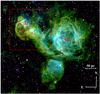 |
Fig. 1 The giant H ii complex LHA 120-N 51 in the light of [S ii] (red), Hα (green), and [O iii] (blue), all data from MCELS (see Sect. 2.3). The red box delineates the area shown in Fig. 2. Noticeable substructures are : DEM L205 (A), the SNR candidate analysed in this paper; N51A (B) and N51C (C, also named DEM L201), two H ii regions also seen in the radio and the IR; the SB N51D, or DEM L192, in (D). |
2.3. Optical
We used data from the Magellanic Clouds Emission Line Survey (MCELS, e.g. Smith et al. 2000). A 8° × 8° region centred on the LMC was observed with the 0.6 m Curtis Schmidt telescope from the University of Michigan/Cerro Tololo Inter-American Observatory (CTIO), using the three narrow-band filters [S ii]λλ6716, 6731 Å, Hα, and [O iii]λ5007 Å and matching red and green continuum filters. We flux-calibrated and combined all MCELS data covering the SNR, with a pixel size of 2′′ × 2′′. The [S ii] and Hα images were stellar continuum-subtracted to produce a map of [S ii]/Hα, which is an efficient criterion for distinguishing SNRs from H ii regions, where the ratio is typically >0.4 and ≲ 0.1, respectively (Fesen et al. 1985). The X-ray composite image and [S ii]/Hα contours from these data are shown in Fig. 2. In addition, we present an unpublished higher-resolution Hα image in Fig. 6 (pixel size of 1′′ × 1′′), which was obtained as part of the ongoing MCELS2 program with the MOSAIC ii camera on the Blanco 4-m telescope at the CTIO.
2.4. Infrared
During the SAGE survey (Meixner et al. 2006), the Spitzer Space Telescope observed a 7° × 7° area in the LMC with the Infrared Array Camera (IRAC; Fazio et al. 2004) in its 3.6, 4.5, 5.8, and 8 μm bands, and with the Multiband Imaging Photometer (MIPS; Rieke et al. 2004) in its 24, 70, and 160 μm bands. To study the IR emission of the source and its environment, we retrieved the IRAC and MIPS mosaiced, flux-calibrated (in units of MJy sr-1) images processed by the SAGE team. The pixel sizes are 0.6′′ for all IRAC wavelengths and 2.49′′ and 4.8′′ for 24 μm and 70 μm MIPS data, respectively.
3. Data analysis and results
3.1. X-rays
3.1.1. Imaging
We created composite images, using the energy ranges 0.2−1 keV for the red component, 1−2 keV for the green, 2−4.5 keV for the blue. The X-ray image is shown in Fig. 2. In addition to soft diffuse emission and many point sources, an extended soft source is clearly seen. This source correlates with the positions of [HP99] 534 and DEM L205. The images alone already show that the source has hardly any emission above 1 keV.
The X-ray emission can be clearly delineated by an ellipse centred at RA = 05h28m05s and Dec = −67°27′20′′, with a position angle of 30° (with respect to the north and towards the east, see Fig. 2). The major and minor axes have sizes of 5.4′ and 4.4′, respectively. At a distance of 50 kpc, this corresponds to an extent of ~79 × 64 pc. We note that the eastern and southern boundaries of the X-ray emission are more clearly defined than the western and northern ones. We discuss this issue in Sect. 4.3.
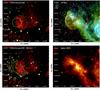 |
Fig. 2 A multicolour view of DEM L205. Top left: X-ray colour image of the remnant, combining all EPIC cameras. Data from two overlapping observations are combined and smoothed (see Sect. 3.1.1 for details). The red, green, and blue components are soft, medium, and hard X-rays, as defined in the text. The white circle is the 90% confidence error of the [HP99] 534 position and the green cross is the central position of DEM L205. The green dashed ellipse (defined in Sect. 3.1.1) encompasses the X-ray emission and is used to define the nominal centre and extent of the remnant. Top right: the same region of the sky in the light of [S ii] (red), Hα (green), and [O iii] (blue), where all data are from the MCELS. The soft X-ray contours from the top left image are overlaid. Bottom left: same EPIC image as above but with [S ii]-to-Hα ratio contours from MCELS data. Levels are (inwards) 0.4, 0.45, 0.5, 0.6, and 0.7. Bottom right: the remnant as seen at 24 μm by Spitzer MIPS. Optical and IR images are displayed logarithmically. |
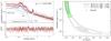 |
Fig. 3 Left: EPIC-pn spectrum of DEM L205. The spectra in the background and source regions (grey and red data points, respectively) are modelled simultaneously. The background model components are shown by the dashed lines and labelled. The Sedov model used for the remnant is shown by the blue solid line. Residuals are shown in the lower panel in terms of σ. Right: the kT – τ parameter plane for the Sedov model. The 68, 90, and 95% CL contours are shown by the solid, dashed, and dotted black lines, respectively. The formal best-fit, occurring at the upper limit of the ionisation ages of the XSPEC model (5 × 10¹³ s cm-3) is marked by the red plus sign. The red line shows the 99% CL lower contour of emission measure obtained with the APEC model. The green hatching indicates the region where Δχ2 < 4.61 and EM is in the 99% CL range of the APEC model (see Sect. 3.1.3). |
3.1.2. Spectral fitting
We created a vignetting-weighted event list to take into account the effective area variation across the source extent. The spectrum was extracted from a circular region with a radius of 3′ and the same centre as the ellipse defined in Sect. 3.1.1. A nearby region of the same size, free of diffuse emission, was used to extract a background spectrum. Point sources were excluded from the extraction regions. Spectra were rebinned with a minimum of 30 counts per bin to allow the use of the χ2-statistic. The spectral-fitting package XSPEC (Arnaud 1996) version 12.7.0u was used to perform the spectral analysis.
Because of the low surface brightness of the source, the spectrum of the source region (background + source) contains a relatively low number of counts. Constraining the parameters of the source model was therefore challenging. The spectra were extracted from different regions of the detector (even from different CCD chips) that have different responses. Simply subtracting the background spectrum would have led to a further loss in the statistical quality of the source spectrum, hindering the spectral fitting of the source emission. A way to prevent this was to estimate the background using a physically motivated model (although any model fitting the data could in principle be used), and then fit the spectra of the source and background regions simultaneously.
For the X-ray background, we used a three-component model, as in Kuntz & Snowden (2010), which consists of i) an unabsorbed thermal component for the Local Hot Bubble (LHB), ii) an absorbed thermal component to model the Galactic halo emission, and iii) an absorbed power-law to account for non-thermal, unresolved extragalactic background. The spectral index was fixed to 1.46 (Chen et al. 1997). We used photoelectric absorption with the cross-sections taken from Balucinska-Church & McCammon (1992) and assumed the elemental abundances of Wilms et al. (2000).
In addition to this X-ray background model, an instrumental fluorescent line of Al Kα, with E = 1.49 keV, and a soft proton contamination (SPC) term were also included. The SPC was modelled by a power-law not convolved with the instrumental response, which is appropriate for photons but not for protons (Kuntz & Snowden 2008).
Three models were used for the emission of the remnant : a thermal plasma, using the Astrophysical Plasma Emission Code (APEC), a plane-parallel shock, and a Sedov model (Borkowski et al. 2001), called vapec, vpshock, and vsedov in XSPEC (where the prefix “v” indicates that abundances can vary). The vsedov model computes the X-ray spectrum of an SNR in the Sedov-Taylor stage of its evolution. The parameters of the Sedov model are the mean shock temperature Ts, the postshock electron temperature Tes and the ionisation timescale τ0, defined as the product of the electron density behind the shock front and the remnant’s age. As Borkowski et al. emphasised, in the case of older and cooler SNRs, only Ts can be determined from spatially integrated X-ray observations with modest spectral resolution. We indeed found little or no variations in the best-fit parameters and the χ2 when constraining β = Tes/Ts between 0 (by taking Tes = 0.01 keV, the minimal value in the Sedov model implemented in XSPEC) and 1. As a consequence, we constrained the mean shock and postshock electron temperature to be the same. This is a reasonable assumption, since old remnants should be close to ion-electron temperature equilibrium.
The vpshock model parameters are the shock temperature and the upper limit to the linear distribution of ionisation timescales τup. This model has been shown to approximate the Sedov model better than the commonly used non-equilibrium ionisation (NEI) model (Borkowski et al. 2001). There are deviations between vpshock and vsedov models for low-temperature shocks, but these occur predominantly above 2 keV.
When fitted to the source region spectrum, the normalisations of the X-ray background components were allowed to vary, but their ratios were constrained to be the same as in the background region. We found 5 % or smaller variations between the normalisations of the background components of the two regions (which are shown by the dashed lines in Fig. 3). Because the background spectrum was extracted from the same observation (that is, at the same time period) and at a similar position and off-axis angle as the source spectrum, the SPC contribution was not expected to vary much (Kuntz & Snowden 2008). The validity of this assumption was checked a posteriori by looking at our data above 3 keV. We therefore used the same SPC parameters for the background and source spectra.
To account for the absorption of the source emission, we included two photoelectric absorption components, one with a column density NH Gal for the Galactic absorption and another one with NH LMC for the LMC. Except for O and Fe, which were allowed to vary, the metal abundances for the source emission models were fixed to the average metallicity in the LMC (i.e., half the solar values, Russell & Dopita 1992), because the observations were not deep enough to permit abundance measurements and because high-resolution spectroscopic data were unavailable.
3.1.3. Spectral results
We fitted the data between 0.2 keV and 7 keV. We extended the fit down to low energies to constrain the parameters of the LHB component, which had a low plasma temperature (kT ≲ 0.1 keV). The data above 2 keV, where the Galactic components hardly contribute, were necessary to constrain the non-thermal extragalactic emission and the SPC (Kuntz & Snowden 2010).
The quality of our data statistics was too low to place strong constraints on the foreground hydrogen absorption column. The best fit value for NH Gal was 5.3 × 1020 cm-2 (using the APEC component), with a 90% confidence interval from 3 to 10 × 1020 cm-2. We therefore fixed it at 5.9 × 1020 cm-2 (based on the H i measurement of Dickey & Lockman 1990). We found that the best-fit intrinsic LMC column density value tended to 0, with a 90% confidence upper limit of 3.9 × 1020 cm-2 (using the APEC component), and then fixed NH LMC to 0. We note that even though the best-fit temperature of the Local Hot Bubble we derived (85 eV) agrees well with the results of Henley & Shelton (2008), the errors are large because this component contributes only to a small number of energy bins. The significance of the LHB component was less than 10% (using a standard F-test), and we removed this component from our final analysis. The power-law component was also faint but more than 99.99% significant.
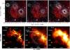 |
Fig. 4 Top row: radio contours of DEM L205 overlaid on the X-ray image. Left: 36 cm contours from 5 to 50σ with 5σ steps (σ = 0.4 mJy/beam). Middle: 20 cm contours from 3 to 23σ with 2σ steps (σ = 1.3 mJy/beam). Right: 6 cm contours from 3 to 200σ with 9σ steps (σ = 0.1 mJy/beam). Beam sizes are 40′′ × 40′′ for the 36 and 20 cm images, and 41.8′′ × 28.5′′ at 6 cm. Note that the portion of the sky shown is smaller than in Fig. 2. Bottow row: Spitzer images of DEM L205 at 8, 24, and 70 μm (from left to right). All images show a similar portion of the sky as the radio images and are displayed logarithmically. The green ellipses on the 8 μm image show the positions of the two H ii regions seen in the 36 cm image (top left), and the cyan arcs indicate the 8 μm emission possibly associated with the SNR. The white dashed line shown in the 24 μm image marks the region where we measured the flux densities at 24 μm and 70 μm (Sect. 3.3). Soft X-ray contours are overlaid in cyan. |
We achieved good fits and obtained significant constraints on the source parameters. The reduced χ2 were between 0.91 and 0.92. The plasma temperatures (kT between 0.2 keV and 0.3 keV) are consistent for all models. They are similar to temperatures found in other extensive SNRs (e.g. Williams et al. 2004; Klimek et al. 2010). The unabsorbed X-ray luminosity of the Sedov model is 1.43 × 1035 erg s-1 in the range 0.2−5 keV, whilst the other models yield similar values. More than 90% of the energy is released below 0.9 keV.
The best-fit values with 90% confidence levels (CL) errors are listed in Table 2. The spectrum fitted by the best-fit Sedov model is shown in Fig. 3. The ionisation timescales were large (more than 1012 s cm-3), which indicates quasi-equilibrium. In this regime, kT and τ are degenerate, because the spectra hardly change when increasing kT and decreasing τ. This effect is shown in Fig. 3. However, the emission measure (EM), which is a function of the volume of emitting plasma and densities, does not depend on the model used, provided the column density is the same. With the help of the 99% CL range of EM obtained using the APEC model (16.0−25.4 × 1057 cm-3), which does not have the kT – τ degeneracy problem, we obtained additional constraints on kT and τ.
The O and Fe abundances are (about 0.2 dex) lower than those in Russell & Dopita (1992) but consistent with the results found by Hughes et al. (1998) in other LMC SNRs. The abundances found for DEM L205 match well those reported in the nearby (13′ or ~190 pc in projection) LMC SB N 51D (Yamaguchi et al. 2010).
3.2. Radio
3.2.1. Morphology
To assess the morphology of the source, we overlaid the radio contours on the XMM-Newton image. Weak, extended ring-like emission correlates with the eastern side of the X-ray remnant and is most prominent, as expected, at 36 cm, but only marginally detected at higher frequencies (Fig. 4, top). It is difficult to classify the morphology of this SNR at radio wavelengths because it lies in a crowded field. The surrounding radio emission is dominated in the north by LHA 120-N 51A, which is classified as an H ii region (Filipovic et al. 1998) and also correlates with the small molecular cloud [FKM2008] LMC N J0528−6726 (Fukui et al. 2008), and in the west by the H ii region LHA 120-N 51C.
If we assumed that the analysable region of the 36 cm image (Fig. 4, top left) is typical of the rest of the remnant’s structure, the SNR would have a typical ring morphology. Nevertheless, with the present resolution, one cannot easily estimate the total flux density of this SNR at any radio frequency. However, we note the steep drop (across the eastern side of the ring) in flux density at higher frequencies, which results in a nearly completely dissipated remnant as seen at 6 cm (Fig. 4, top right).
3.2.2. Radio-continuum spectral energy distribution
We were unable to compile a global spectral index for the remnant because a large portion of DEM L205 cannot be analysed at radio wavelengths (as described in Sect. 3.2.1). However, a spectral index map (Fig. 5) shows the change in flux density from 36 cm to 6 cm. The map was formed by reprocessing all observations to a common u − v range, and then fitting S ∝ ν α pixel by pixel using all three images simultaneously. The areas of the SNR that are uncontaminated by strong sources have spectral indices between −0.7 and −0.9, which is steeper but close to the typical SNR radio-continuum spectral index of α ~−0.5. We note that uncertainties in the determination of the background emission are likely to cause a bias toward steeper spectral indices. We also point out that the bright point source seen in the north-east (mainly at 36 cm) is most likely a background galaxy or an active galactic nucleus (AGN).
3.3. Infrared flux measurement
The IR data suffer from the same crowding issues as the radio-continuum data. The IR emission in the SNR region (see Fig. 4, bottom) is dominated by the two H ii regions seen in radio, whose positions are shown in the 8 μm images (Fig. 4, bottom left). However, at 24 μm, an arc of shell-like emission is seen in the eastern and south-eastern regions of the remnant (outlined in Fig. 4, bottom middle) at the same position of the 36 cm emission. We used the optical and X-ray emission contours to constrain the region at 24 μm that can be truly associated with the SNR and found that this arc tightly follows the Hα and X-ray morphologies. We integrated the 24 μm surface brightness in this region (in white in Fig. 4, bottom middle) and found a flux density of F24 = 660 mJy.
To calibrate our method of flux density measurement and estimate the uncertainties, we derived the 24 μm flux densities of the LMC SNRs N132D, N23, N49B, B0453–68.5, and DEM L71, and compared them to the values published in Borkowski et al. (2006) and Williams et al. (2006). We were able to reproduce these authors’ values, but with rather large error ranges (~30%), chiefly because of uncertainties in the definition of the integration region. The two aforementioned studies integrated the flux density only in limited areas of the SNRs, and the integration regions are not explicitly defined in their papers. In the case of DEM L205 it is also difficult to define the area of IR emission from the SNR only, so we believe these 30% error ranges are a reasonable estimate of the error in the flux density measurement. The systematic uncertainties in the flux calibration of the Spitzer images are small in comparison and can be neglected. In particular, given that the thickness of our region in the plane of the sky is 20′′–25′′, only a small aperture correction would be needed (at least at 24 μm).
The 70 μm image (Fig. 4, bottom right) shows that DEM L205 has the same morphology as at 24 μm, but with lower resolution, hence the confusion is even higher. Simply using the same region as for F24, we found a flux density of F70 = 3.4 Jy, with similarly large errors. We discuss the origin of the IR emission in Sect. 4.1.
In the IRAC wavebands, no significant shell-like emission is detected. We tentatively identified two arcs at 8 μm (marked in cyan in Fig. 4, bottom left) that could originate from the interaction of the shock with higher densities towards the H ii regions. The two arcs are also present at 5.8 μm (not shown) but neither at 4.5 μm nor 3.6 μm, where only point sources are seen.
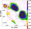 |
Fig. 5 Spectral index map of DEM L205 between wavelength of 36, 20, and 6 cm, covering the same field as Fig. 4. The sidebar gives the spectral index α, as defined in the introduction. The 36 cm contours (black) are overlaid, with the same levels as in Fig. 4. The Hα structures (Figs. 1 and 2) are sketched by the magenta contours. |
4. Discussion
Since the source exhibits all the classical SNR signatures, we can confirm DEM L205 as a new supernova remnant. This brings the total number of SNRs in the LMC to 56, using the list of 54 remnants assembled by Badenes et al. (2010) and the new SNR identified by Grondin et al. (2012). For the naming of SNRs in the Magellanic Clouds, we advocate the use of the acronym “MCSNR”, which was pre-registered to the International Astronomical Union by Williams et al., who maintain the Magellanic Cloud Supernova Remnants online database2. This should ensure that there is a more consistent and general naming system for future studies using the whole sample of SNRs in the LMC. On the basis of the J2000 X-ray position, DEM L205 would thus be called MCSNR J0528−6727.
In the following sections, we take advantage of the multi-wavelength observations of the remnant and discuss the origin of the IR emission (Sect. 4.1), derive some physical properties of the remnant (Sect. 4.2), compare the morphology at all observed wavelengths and discuss the environment in which the SN exploded (Sect. 4.3), and analyse the star formation activity around the SNR (Sect. 4.4).
4.1. Origin of the IR emission
Supernova remnants emit IR light chiefly in forbidden lines, rotational/vibrational lines of molecular hydrogen, emission in polycyclic aromatic hydrocarbon (PAH) bands, and thermal continuum emission from dust collisionally heated by shock waves (e.g. Koo et al. 2007) and/or by stellar-radiation reprocessing. Infrared synchrotron emission is only expected in pulsar wind nebulae, for instance in the Crab (Temim et al. 2006). Polycyclic aromatic hydrocarbons are thought to be destroyed by shocks with velocities higher than 100 km s-1 and should not survive for more than a thousand years in a tenuous hot gas (Micelotta et al. 2010a,b). However, PAH features have been detected in Galactic SNRs (Andersen et al. 2011), where shock velocities are rather low owing to interactions with a molecular cloud environment, and even in the strong shocks of the young LMC remnant N132D (Tappe et al. 2006).
No significant emission from DEM L205 was detected in the IRAC wavebands (which have been chosen to include the main PAH features), with the possible exception of the two 8 and 5.8 μm arcs (Fig. 4, bottom left) in the direction of the neighbouring H ii regions (in the north and west). This means that PAHs have been efficiently destroyed. The absence of IR spectroscopic observations precludes further interpretation.
The presence of Hα emission shows that hydrogen is not in the molecular phase, hence rotational/vibrational line contribution is negligible. The emission in the 24 and 70 μm wavebands should then be dominated either by dust or ionic forbidden lines. Ionic lines in the 24 μm filter bandpass are [S i] 25.2 μm, [Fe ii] 24.50 and 25.99 μm, [Fe iii] 22.95 μm, and [O iv] 25.91 μm. [S i] emission is not expected because of the prominent [S ii] optical emission, showing that S+ is the primary ionisation stage of sulphur. The morphological similarities between the MIR and X-ray emission lead us to the interpretation that we mainly observe the thermal continuum of dust. The correlation with 70 μm supports this scenario, and the 70-to-24 μm ratio (~5.2) is consistent with a dust temperature of 50−80 K (Williams et al. 2006). We note, however, that in the northern part of the arc of 24 μm emission (encompassed by the white dashed line in Fig. 4, bottom middle), the MIR emission is slightly ahead of the shock (delineated by the X-ray emission), whereas it correlates tightly with the shock in the rest of the arc. This morphology and the presence of the OB association LH 63 (see Fig. 6, right) indicates that stellar radiation dominates the heating of the dust in the north. In the southern part, shock waves could play a more significant role in heating the dust.
The lack of spectroscopic data prevent us from establishing the precise contribution of dust vs. O and Fe lines. Because of these limitations and the confusion with the background, and because only part of the SNR is detected at IR wavelengths, we did not attempt to derive a dust mass. Consequently, no dust-to-gas ratio (using the swept-up gas mass estimate from X-ray observations) and dust destruction percentage can be given.
4.2. Properties of DEM L205 derived from the X-ray observations
From the X-ray spectral analysis, we can derive several physical properties of the
remnant : electron and hydrogen densities ne and
nH, dynamical and ionisation ages
tdyn and ti, swept-up mass
M, and initial explosion energy E0. We used
a system of equations adapted from van der Heyden et al.
(2004), given by 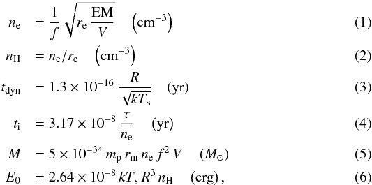 where
EM is the emission measure
(=nenHV)
in cm-3, kTs is the shock
temperature in keV, and τ is the ionisation timescale in
s cm-3. These parameters are determined by the spectral fitting. In addition,
R is the radius of the X-ray remnant in cm (using the semi-major axis
of 39.5 pc, see Sect. 3.1.1), V is
the volume (4π/3 × R3)
assuming spherical symmetry (as discussed below), mp is the
proton mass in g, rm is the total number of baryons per
hydrogen atom
(= nm/nH),
and re is the number of electrons per hydrogen atom
(= ne/nH).
Assuming a plasma with 0.5 solar metal abundances, as done in the spectral fitting, we
have rm ≈ 1.40 and re ≈ 1.20
(for full ionisation). Finally, f is a filling factor to correct for any
departure from spherical symmetry, as inferred from the X-ray morphology.
f is defined as
where
EM is the emission measure
(=nenHV)
in cm-3, kTs is the shock
temperature in keV, and τ is the ionisation timescale in
s cm-3. These parameters are determined by the spectral fitting. In addition,
R is the radius of the X-ray remnant in cm (using the semi-major axis
of 39.5 pc, see Sect. 3.1.1), V is
the volume (4π/3 × R3)
assuming spherical symmetry (as discussed below), mp is the
proton mass in g, rm is the total number of baryons per
hydrogen atom
(= nm/nH),
and re is the number of electrons per hydrogen atom
(= ne/nH).
Assuming a plasma with 0.5 solar metal abundances, as done in the spectral fitting, we
have rm ≈ 1.40 and re ≈ 1.20
(for full ionisation). Finally, f is a filling factor to correct for any
departure from spherical symmetry, as inferred from the X-ray morphology.
f is defined as  ,
where Vt is the true X-ray emitting (ellipsoidal) volume.
Adopting the semi-minor axis of the X-ray emitting ellipse (32 pc) as the second
semi-principal axis, f is in the range 0.81−0.90, with the third
semi-principal axis being between 32 pc and 39.5 pc. The properties are listed in
Table 3, using f in this range
and EM in the range defined in Sect. 3.1.3.
,
where Vt is the true X-ray emitting (ellipsoidal) volume.
Adopting the semi-minor axis of the X-ray emitting ellipse (32 pc) as the second
semi-principal axis, f is in the range 0.81−0.90, with the third
semi-principal axis being between 32 pc and 39.5 pc. The properties are listed in
Table 3, using f in this range
and EM in the range defined in Sect. 3.1.3.
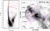 |
Fig. 6 Left: colour–magnitude diagram (CMD) of the MCPS stars (Zaritsky et al. 2004) within 100 pc (~6.9′) of the central position of DEM L205. Geneva stellar evolution tracks (Lejeune & Schaerer 2001) are shown as red lines, for metallicity of 0.4 Z⊙ and initial masses of 3, 5 M⊙ (dashed lines) and 10, 15, 20, 25, and 40 M⊙ (solid lines), from bottom to top. The green dashed line shows the criteria used to identify the OB stars (V < 16 and B − V < 0). Stars satisfying these criteria are shown as blue dots. Right: MCELS2 Hα image of the SNR, with the soft X-ray contours in magenta. The blue plus signs show the positions of the OB candidates identified in the CMD and green squares identify Sanduleak OB stars. The black dashed circles encompass the nearby OB associations 60 and 63 from Lucke & Hodge (1970). Positions of definite (yellow diamond) and probable (red circle) YSOs from Gruendl & Chu (2009) are also shown. |
The large amount (from 400 M⊙ to 460 M⊙) of swept-up gas justifies a posteriori that the SNR is indeed well-established in the Sedov phase. Because the remnant is old, the plasma is close to or in collisional ionisation equilibrium, as indicated by either the acceptable fit of the APEC model or the large ionisation timescale τ, for which only a lower limit is found. Thus, the spectrum changes very slowly with time and τ is no longer a sensitive age indicator (van der Heyden et al. 2004). This explains why ti is unrealistically long (>770 kyr, from Eqs. (1) and (4)) and unreliable.
4.3. Multi-wavelength morphology
In Fig. 2, we see an X-ray remnant with a slightly elongated shape and a maximal extent of 79 pc. Therefore, DEM L205 ranks amongst the largest known in the LMC (compared e.g. to SNRs described in Cajko et al. 2009; Klimek et al. 2010; Grondin et al. 2012). The optical emission-line images (Figs. 2 and 6) show the shell-like structure of DEM L205 coinciding with the boundary of the X-ray emission from the remnant. Dunne et al. (2001) classified the shell as a SB, interpreting the morphology of DEM L205 as a blister blown by the OB association LH 63 (see Sect. 4.4 and Fig. 6, right). They measured a mild expansion velocity of ~70 km s-1 for the Hα shell, which is typical of SBs. Supernova remnants exhibit higher expansion velocities (≳ 100 km s-1), although this is not a necessary condition (Chu 1997).
On the basis of the low densities (<0.1 cm-3) derived from the X-ray spectral analysis, we conclude that the supernova exploded inside the blister, producing the bright X-ray emission in the interior of the SB. The SNR shocks reaching the inner edge of the bubble might then have produced non-thermal radio emission, and the observed morphology at 36 cm is consistent with this picture.
The remnant is located in a complex environment. In the north and west, we detected two H ii regions and a strip of dust and gas extending down towards the south-west. The H ii regions also show bright IR emission, mainly from dust heated by stellar radiation, and bright (thermal) radio-continuum emission (Fig. 4). The [S ii]-to-Hα ratio is higher in the south of the remnant, indicating that the diffuse optical emission there is caused by the SNR shocks. In addition, the lower ratio in the north and west parts of the remnant is most likely due to photoionisation by the massive stars (bringing sulphur to ionisation stages higher than S+) from the same OB associations that power the H ii regions and produced the SB in which the supernova exploded. We therefore propose that the SNR and the H ii regions are physically connected.
Furthermore, whilst the X-ray surface brightness falls abruptly across the eastern and southern boundaries of the remnant, much weaker emission is detected in the north and west, right at the positions of the H ii regions seen at all other wavelengths (Figs. 2 and 4). This indicates that the remnant is behind the H ii regions. The absorption column density is higher in the north and west, suppressing the X-ray emission and giving rise to the observed asymmetrical, irregular shape in these regions. The ellipse defined in Sect. 3.1.1 is probably an oversimplification of the actual morphology of the X-ray emitting region. The remnant may have a more spherical shape, with some parts masked by the H ii regions.
We also detected soft and faint diffuse X-ray emission on the other side of the dust/gas strip. The diffuse X-ray emission is enclosed by very sharp and faint Hα filaments (Figs. 2 and 6). The presence of the OB association (LH 60) suggests that we observed another stellar-wind-blown SB in which a SN had exploded. The faintness of the X-ray and optical emission precludes further analysis. We note here that the [S ii]-to-Hα ratio is <0.4. However, it cannot be used in that case because of the presence of massive stars from the OB association.
4.4. Past and present star formation activity around the SNR
The star formation history (SFH) and high-mass-star content of the local environment of DEM L205 can help us to determine whether the remnant’s supernova progenitor type is either thermonuclear (type Ia) or core-collapse (CC). The latter originates from massive stars that rarely form in isolation. Therefore, the combination of a recent peak in the star formation rate and the presence of many early-type stars is expected in the case of CC SNe, whereas the contrary would be more consistent with a type Ia SN.
To investigate the star content around the remnant, we used the Magellanic Clouds Photometric Survey (MCPS) catalogue of Zaritsky et al. (2004) and constructed the colour-magnitude diagram (CMD) of the ~20 000 stars lying within 100 pc (6.9′) of the remnant’s centre. The CMD (Fig. 6, left) shows a prominent upper main-sequence branch. We added stellar evolutionary tracks of Lejeune & Schaerer (2001), for Z = 0.4 Z⊙ and initial masses from 3 M⊙ to 40 M⊙, assuming a distance modulus of 18.49 and extinction AV = 0.5 (the average extinction for “hot” stars, Zaritsky et al. 2004). We used the criteria of V < 16 and B − V < 0 to identify OB stars, and found 142 of them in our sample (shown in a Hα image in Fig. 6, right). Using V < 15 or 14 instead of 16 would give 86 and 20 stars, respectively.
We also looked for nearby OB associations in Lucke & Hodge (1970) and OB stars in the catalogue of Sanduleak (1970). Contamination by Galactic stars was monitored by performing a cross-correlation with Tycho-2 stars (Høg et al. 2000). Five Sanduleak stars are in this region, four of them having a match in the MCPS catalogue, with our selection criteria. The “missed” Sanduleak star is a VV Cepheid (a binary with a red component), which thus possibly explains why our criteria were not satisfied. Two OB associations (LH 60 and 63) lie close to the remnant (~6′ and 3′, respectively), and their extent indeed contain many OB stars from the MCPS catalogue.
Harris & Zaritsky (2008) performed a spatially resolved analysis of the SFH of the “Constellation III” region, and DEM L205 was included in their study (the “E00” cell in their Fig. 2). They identified that a very strong peak in the star formation rate occurred in the region of the remnant 10 Myr ago, and that little star formation activity had occurred prior to this burst.
The rich content of high-mass stars and the recent peak in SFH around the remnant strongly suggest that a core-collapse supernova has formed DEM L205. It is however impossible to completely rule out a type Ia event. Considering at face value that most of the stars were formed in the SFR peak 10 Myr ago, we estimated a lower limit for the mass of the SN progenitor of 20 M⊙, because less massive stars have a lifetime longer than 10 Myr (Meynet et al. 1994). We cannot estimate an upper limit, because the progenitor might have formed more recently (the region is still actively forming stars, see below).
We searched for nearby young stellar objects (YSOs) to assess the possibility of SNR-triggered star formation, as in Desai et al. (2010). Using the YSOs from the catalogue of Gruendl & Chu (2009), we report an SNR – molecular cloud – YSOs association around DEM L205: the positions of young stars are shown in our Hα image (Fig. 6, right). Four YSOs lie in the H ii region/molecular cloud in the north, and are closely aligned with the X-ray emission rim. In addition, four YSOs lie in the western H ii region, significantly beyond the remnant’s emission but correlated with the diffuse X-ray emission from the SB around LH 60 (see Sect. 4.3). Two additional YSOs are aligned with the south-western edge of the SB.
Given the contraction timescale for the intermediate to massive YSOs (106 yr to 105 yr, Bernasconi & Maeder 1996), the shocks from the remnant cannot have triggered the formation of the YSOs already present. These YSOs are more likely to have formed by interactions with winds and ionisation fronts from the local massive stars, as illustrated by the alignment of young stars along the rim of the adjacent SB. The remnant will be able to trigger star formation in the future, when the shocks have slowed down to below 45 km s-1 (Vanhala & Cameron 1998). By this time, however, the neighbouring massive stars will also have triggered further star formation. It is therefore difficult to assess the exact triggering agent of star formation, as Desai et al. (2010) pointed out, in particular in such a complex environment.
5. Conclusions
The first observation of our LMC survey with XMM-Newton included the SNR candidate DEM L205 in the field of view. In combination with unpublished radio-continuum data and archival optical and IR observations, we have found all classical SNR signatures, namely:
-
Extended X-ray emission.
-
Optical emission with a shell-like morphology and an enhanced [S ii]-to-Hα ratio.
-
Non-thermal and extended radio-continuum emission.
Science Analysis Software, http://xmm.esac.esa.int/sas/
Acknowledgments
The XMM-Newton project is supported by the Bundesministerium für Wirtschaft und Technologie/Deutsches Zentrum für Luft- und Raumfahrt (BMWi/DLR, FKZ 50 OX 0001) and the Max-Planck Society. Cerro Tololo Inter-American Observatory (CTIO) is operated by the Association of Universities for Research in Astronomy Inc. (AURA), under a cooperative agreement with the National Science Foundation (NSF) as part of the National Optical Astronomy Observatories (NOAO). We gratefully acknowledge the support of CTIO and all the assistance which has been provided in upgrading the Curtis Schmidt telescope. The MCELS is funded through the support of the Dean B. McLaughlin fund at the University of Michigan and through NSF grant 9540747. The Australia Telescope Compact Array is part of the Australia Telescope which is funded by the Commonwealth of Australia for operation as a National Facility managed by CSIRO. We used the karma software package developed by the ATNF. This research has made use of Aladin, SIMBAD and VizieR, operated at CDS, Strasbourg, France. Pierre Maggi thanks Philipp Lang for helpful discussions regarding IR data analysis. P.M. and R.S. acknowledge support from the BMWi/DLR grants FKZ 50 OR 1201 and FKZ OR 0907, respectively. R.A.G. was partially supported by the NSF grant AST 08-07323.
References
- Andersen, M., Rho, J., Reach, W. T., Hewitt, J. W., & Bernard, J. P. 2011, ApJ, 742, 7 [NASA ADS] [CrossRef] [Google Scholar]
- Arnaud, K. A. 1996, in Astronomical Data Analysis Software and Systems V, eds. G. H. Jacoby, & J. Barnes, ASP Conf. Ser., 101, 17 [Google Scholar]
- Badenes, C., Maoz, D., & Draine, B. T. 2010, MNRAS, 407, 1301 [NASA ADS] [CrossRef] [Google Scholar]
- Balucinska-Church, M., & McCammon, D. 1992, ApJ, 400, 699 [NASA ADS] [CrossRef] [Google Scholar]
- Bernasconi, P. A., & Maeder, A. 1996, A&A, 307, 829 [NASA ADS] [Google Scholar]
- Borkowski, K. J., Lyerly, W. J., & Reynolds, S. P. 2001, ApJ, 548, 820 [NASA ADS] [CrossRef] [Google Scholar]
- Borkowski, K. J., Williams, B. J., Reynolds, S. P., et al. 2006, ApJ, 642, L141 [NASA ADS] [CrossRef] [Google Scholar]
- Cajko, K. O., Crawford, E. J., & Filipovic, M. D. 2009, Serb. Astron. J, 179, 55 [Google Scholar]
- Chen, L.-W., Fabian, A. C., & Gendreau, K. C. 1997, MNRAS, 285, 449 [NASA ADS] [CrossRef] [Google Scholar]
- Chu, Y.-H. 1997, AJ, 113, 1815 [NASA ADS] [CrossRef] [Google Scholar]
- Davies, R. D., Elliott, K. H., & Meaburn, J. 1976, MmRAS, 81, 89 [Google Scholar]
- de Horta, A. Y., Filipović, M. D., Bozzetto, L. M., et al. 2012, A&A, 540, A25 [NASA ADS] [CrossRef] [EDP Sciences] [Google Scholar]
- Desai, K. M., Chu, Y.-H., Gruendl, R. A., et al. 2010, AJ, 140, 584 [NASA ADS] [CrossRef] [Google Scholar]
- di Benedetto, G. P. 2008, MNRAS, 390, 1762 [NASA ADS] [Google Scholar]
- Dickel, J. R., McIntyre, V. J., Gruendl, R. A., & Milne, D. K. 2005, AJ, 129, 790 [NASA ADS] [CrossRef] [Google Scholar]
- Dickel, J. R., McIntyre, V. J., Gruendl, R. A., & Milne, D. K. 2010, AJ, 140, 1567 [NASA ADS] [CrossRef] [Google Scholar]
- Dickey, J. M., & Lockman, F. J. 1990, ARA&A, 28, 215 [NASA ADS] [CrossRef] [MathSciNet] [Google Scholar]
- Dunne, B. C., Points, S. D., & Chu, Y.-H. 2001, ApJS, 136, 119 [NASA ADS] [CrossRef] [Google Scholar]
- Fazio, G. G., Hora, J. L., Allen, L. E., et al. 2004, ApJS, 154, 10 [NASA ADS] [CrossRef] [Google Scholar]
- Fesen, R. A., Blair, W. P., & Kirshner, R. P. 1985, ApJ, 292, 29 [NASA ADS] [CrossRef] [Google Scholar]
- Filipovic, M. D., Haynes, R. F., White, G. L., & Jones, P. A. 1998, A&AS, 130, 421 [NASA ADS] [CrossRef] [EDP Sciences] [Google Scholar]
- Fukui, Y., Kawamura, A., Minamidani, T., et al. 2008, ApJS, 178, 56 [NASA ADS] [CrossRef] [Google Scholar]
- Grondin, M.-H., Sasaki, M., Haberl, F., et al. 2012, A&A, 539, A15 [NASA ADS] [CrossRef] [EDP Sciences] [Google Scholar]
- Gruendl, R. A., & Chu, Y.-H. 2009, ApJS, 184, 172 [Google Scholar]
- Haberl, F., & Pietsch, W. 1999, A&AS, 139, 277 [NASA ADS] [CrossRef] [EDP Sciences] [Google Scholar]
- Harris, J., & Zaritsky, D. 2008, PASA, 25, 116 [Google Scholar]
- Henize, K. G. 1956, ApJS, 2, 315 [NASA ADS] [CrossRef] [Google Scholar]
- Henley, D. B., & Shelton, R. L. 2008, ApJ, 676, 335 [NASA ADS] [CrossRef] [Google Scholar]
- Høg, E., Fabricius, C., Makarov, V. V., et al. 2000, A&A, 355, L27 [NASA ADS] [Google Scholar]
- Hughes, J. P., Hayashi, I., & Koyama, K. 1998, ApJ, 505, 732 [NASA ADS] [CrossRef] [Google Scholar]
- Hughes, A., Staveley-Smith, L., Kim, S., Wolleben, M., & Filipović, M. 2007, MNRAS, 382, 543 [NASA ADS] [CrossRef] [Google Scholar]
- Klimek, M. D., Points, S. D., Smith, R. C., Shelton, R. L., & Williams, R. 2010, ApJ, 725, 2281 [NASA ADS] [CrossRef] [Google Scholar]
- Koo, B.-C., Lee, H.-G., Moon, D.-S., et al. 2007, PASJ, 59, 455 [NASA ADS] [Google Scholar]
- Kuntz, K. D., & Snowden, S. L. 2008, A&A, 478, 575 [NASA ADS] [CrossRef] [EDP Sciences] [Google Scholar]
- Kuntz, K. D., & Snowden, S. L. 2010, ApJS, 188, 46 [NASA ADS] [CrossRef] [Google Scholar]
- Lejeune, T., & Schaerer, D. 2001, A&A, 366, 538 [NASA ADS] [CrossRef] [EDP Sciences] [Google Scholar]
- Lucke, P. B., & Hodge, P. W. 1970, AJ, 75, 171 [NASA ADS] [CrossRef] [Google Scholar]
- Mathewson, D. S., & Clarke, J. N. 1973, ApJ, 180, 725 [NASA ADS] [CrossRef] [Google Scholar]
- Meixner, M., Gordon, K. D., Indebetouw, R., et al. 2006, AJ, 132, 2268 [NASA ADS] [CrossRef] [Google Scholar]
- Meynet, G., Maeder, A., Schaller, G., Schaerer, D., & Charbonnel, C. 1994, A&AS, 103, 97 [NASA ADS] [Google Scholar]
- Micelotta, E. R., Jones, A. P., & Tielens, A. G. G. M. 2010a, A&A, 510, A37 [NASA ADS] [CrossRef] [EDP Sciences] [Google Scholar]
- Micelotta, E. R., Jones, A. P., & Tielens, A. G. G. M. 2010b, A&A, 510, A36 [NASA ADS] [CrossRef] [EDP Sciences] [Google Scholar]
- Mills, B. Y., Turtle, A. J., Little, A. G., & Durdin, J. M. 1984, Austr. J. Phys., 37, 321 [Google Scholar]
- Rieke, G. H., Young, E. T., Engelbracht, C. W., et al. 2004, ApJS, 154, 25 [NASA ADS] [CrossRef] [Google Scholar]
- Russell, S. C., & Dopita, M. A. 1992, ApJ, 384, 508 [NASA ADS] [CrossRef] [Google Scholar]
- Sanduleak, N. 1970, Contributions from the Cerro Tololo Inter-American Observatory, 89 [Google Scholar]
- Smith, C., Leiton, R., & Pizarro, S. 2000, in Stars, Gas and Dust in Galaxies: Exploring the Links, eds. D. Alloin, K. Olsen, & G. Galaz, ASP Conf. Ser., 221, 83 [Google Scholar]
- Strüder, L., Briel, U., Dennerl, K., et al. 2001, A&A, 365, L18 [NASA ADS] [CrossRef] [EDP Sciences] [Google Scholar]
- Tappe, A., Rho, J., & Reach, W. T. 2006, ApJ, 653, 267 [NASA ADS] [CrossRef] [Google Scholar]
- Temim, T., Gehrz, R. D., Woodward, C. E., et al. 2006, AJ, 132, 1610 [NASA ADS] [CrossRef] [Google Scholar]
- Turner, M. J. L., Abbey, A., Arnaud, M., et al. 2001, A&A, 365, L27 [NASA ADS] [CrossRef] [EDP Sciences] [Google Scholar]
- van der Heyden, K. J., Bleeker, J. A. M., & Kaastra, J. S. 2004, A&A, 421, 1031 [NASA ADS] [CrossRef] [EDP Sciences] [Google Scholar]
- Vanhala, H. A. T., & Cameron, A. G. W. 1998, ApJ, 508, 291 [NASA ADS] [CrossRef] [Google Scholar]
- Watson, M. G., Schröder, A. C., Fyfe, D., et al. 2009, A&A, 493, 339 [NASA ADS] [CrossRef] [EDP Sciences] [Google Scholar]
- Williams, R. M., Chu, Y.-H., Dickel, J. R., et al. 2004, ApJ, 613, 948 [NASA ADS] [CrossRef] [Google Scholar]
- Williams, B. J., Borkowski, K. J., Reynolds, S. P., et al. 2006, ApJ, 652, L33 [NASA ADS] [CrossRef] [Google Scholar]
- Wilms, J., Allen, A., & McCray, R. 2000, ApJ, 542, 914 [NASA ADS] [CrossRef] [Google Scholar]
- Yamaguchi, H., Sawada, M., & Bamba, A. 2010, ApJ, 715, 412 [NASA ADS] [CrossRef] [Google Scholar]
- Zaritsky, D., Harris, J., Thompson, I. B., & Grebel, E. K. 2004, AJ, 128, 1606 [NASA ADS] [CrossRef] [Google Scholar]
All Tables
All Figures
|
Fig. 1 The giant H ii complex LHA 120-N 51 in the light of [S ii] (red), Hα (green), and [O iii] (blue), all data from MCELS (see Sect. 2.3). The red box delineates the area shown in Fig. 2. Noticeable substructures are : DEM L205 (A), the SNR candidate analysed in this paper; N51A (B) and N51C (C, also named DEM L201), two H ii regions also seen in the radio and the IR; the SB N51D, or DEM L192, in (D). |
| In the text | |
|
Fig. 2 A multicolour view of DEM L205. Top left: X-ray colour image of the remnant, combining all EPIC cameras. Data from two overlapping observations are combined and smoothed (see Sect. 3.1.1 for details). The red, green, and blue components are soft, medium, and hard X-rays, as defined in the text. The white circle is the 90% confidence error of the [HP99] 534 position and the green cross is the central position of DEM L205. The green dashed ellipse (defined in Sect. 3.1.1) encompasses the X-ray emission and is used to define the nominal centre and extent of the remnant. Top right: the same region of the sky in the light of [S ii] (red), Hα (green), and [O iii] (blue), where all data are from the MCELS. The soft X-ray contours from the top left image are overlaid. Bottom left: same EPIC image as above but with [S ii]-to-Hα ratio contours from MCELS data. Levels are (inwards) 0.4, 0.45, 0.5, 0.6, and 0.7. Bottom right: the remnant as seen at 24 μm by Spitzer MIPS. Optical and IR images are displayed logarithmically. |
| In the text | |
|
Fig. 3 Left: EPIC-pn spectrum of DEM L205. The spectra in the background and source regions (grey and red data points, respectively) are modelled simultaneously. The background model components are shown by the dashed lines and labelled. The Sedov model used for the remnant is shown by the blue solid line. Residuals are shown in the lower panel in terms of σ. Right: the kT – τ parameter plane for the Sedov model. The 68, 90, and 95% CL contours are shown by the solid, dashed, and dotted black lines, respectively. The formal best-fit, occurring at the upper limit of the ionisation ages of the XSPEC model (5 × 10¹³ s cm-3) is marked by the red plus sign. The red line shows the 99% CL lower contour of emission measure obtained with the APEC model. The green hatching indicates the region where Δχ2 < 4.61 and EM is in the 99% CL range of the APEC model (see Sect. 3.1.3). |
| In the text | |
|
Fig. 4 Top row: radio contours of DEM L205 overlaid on the X-ray image. Left: 36 cm contours from 5 to 50σ with 5σ steps (σ = 0.4 mJy/beam). Middle: 20 cm contours from 3 to 23σ with 2σ steps (σ = 1.3 mJy/beam). Right: 6 cm contours from 3 to 200σ with 9σ steps (σ = 0.1 mJy/beam). Beam sizes are 40′′ × 40′′ for the 36 and 20 cm images, and 41.8′′ × 28.5′′ at 6 cm. Note that the portion of the sky shown is smaller than in Fig. 2. Bottow row: Spitzer images of DEM L205 at 8, 24, and 70 μm (from left to right). All images show a similar portion of the sky as the radio images and are displayed logarithmically. The green ellipses on the 8 μm image show the positions of the two H ii regions seen in the 36 cm image (top left), and the cyan arcs indicate the 8 μm emission possibly associated with the SNR. The white dashed line shown in the 24 μm image marks the region where we measured the flux densities at 24 μm and 70 μm (Sect. 3.3). Soft X-ray contours are overlaid in cyan. |
| In the text | |
|
Fig. 5 Spectral index map of DEM L205 between wavelength of 36, 20, and 6 cm, covering the same field as Fig. 4. The sidebar gives the spectral index α, as defined in the introduction. The 36 cm contours (black) are overlaid, with the same levels as in Fig. 4. The Hα structures (Figs. 1 and 2) are sketched by the magenta contours. |
| In the text | |
|
Fig. 6 Left: colour–magnitude diagram (CMD) of the MCPS stars (Zaritsky et al. 2004) within 100 pc (~6.9′) of the central position of DEM L205. Geneva stellar evolution tracks (Lejeune & Schaerer 2001) are shown as red lines, for metallicity of 0.4 Z⊙ and initial masses of 3, 5 M⊙ (dashed lines) and 10, 15, 20, 25, and 40 M⊙ (solid lines), from bottom to top. The green dashed line shows the criteria used to identify the OB stars (V < 16 and B − V < 0). Stars satisfying these criteria are shown as blue dots. Right: MCELS2 Hα image of the SNR, with the soft X-ray contours in magenta. The blue plus signs show the positions of the OB candidates identified in the CMD and green squares identify Sanduleak OB stars. The black dashed circles encompass the nearby OB associations 60 and 63 from Lucke & Hodge (1970). Positions of definite (yellow diamond) and probable (red circle) YSOs from Gruendl & Chu (2009) are also shown. |
| In the text | |
Current usage metrics show cumulative count of Article Views (full-text article views including HTML views, PDF and ePub downloads, according to the available data) and Abstracts Views on Vision4Press platform.
Data correspond to usage on the plateform after 2015. The current usage metrics is available 48-96 hours after online publication and is updated daily on week days.
Initial download of the metrics may take a while.