| Issue |
A&A
Volume 543, July 2012
|
|
|---|---|---|
| Article Number | A80 | |
| Number of page(s) | 17 | |
| Section | Stellar atmospheres | |
| DOI | https://doi.org/10.1051/0004-6361/201219034 | |
| Published online | 29 June 2012 | |
Quantitative spectroscopy of Galactic BA-type supergiants
I. Atmospheric parameters⋆,⋆⋆
Dr. Karl Remeis-Sternwarte & ECAP, Universität
Erlangen-Nürnberg, Sternwartstr.
7, 96049
Bamberg, Germany
e-mail: This email address is being protected from spambots. You need JavaScript enabled to view it.
; This email address is being protected from spambots. You need JavaScript enabled to view it.
Received:
14
February
2012
Accepted:
8
May
2012
Abstract
Context. BA-type supergiants show a high potential as versatile indicators for modern astronomy. This paper constitutes the first in a series that aims at a systematic spectroscopic study of Galactic BA-type supergiants. Various problems will be addressed, including in particular observational constraints on the evolution of massive stars and a determination of abundance gradients in the Milky Way.
Aims. The focus here is on the determination of accurate and precise atmospheric parameters for a sample of Galactic BA-type supergiants as prerequisite for all further analysis. Some first applications include a recalibration of functional relationships between spectral-type, intrinsic colours, bolometric corrections and effective temperature, and an exploration of the reddening-free Johnson Q and Strömgren [c1] and β-indices as photometric indicators for effective temperatures and gravities of BA-type supergiants.
Methods. An extensive grid of theoretical spectra is computed based on a hybrid non-LTE approach, covering the relevant parameter space in effective temperature, surface gravity, helium abundance, microturbulence and elemental abundances. The atmospheric parameters are derived spectroscopically by line-profile fits of our theoretical models to high-resolution and high-S/N spectra obtained at various observatories. Ionization equilibria of multiple metals and the Stark-broadened hydrogen and the neutral helium lines constitute our primary indicators for the parameter determination, supplemented by (spectro-)photometry from the UV to the near-IR.
Results. We obtain accurate atmospheric parameters for 35 sample supergiants from a homogeneous analysis. Data on effective temperatures, surface gravities, helium abundances, microturbulence, macroturbulence and rotational velocities are presented. The interstellar reddening and the ratio of total-to-selective extinction towards the stars are determined. Our empirical spectral-type–Teff scale is steeper than reference relations from the literature, the stars are significantly bluer than usually assumed, and bolometric corrections differ significantly from established literature values. Photometric Teff-determinations based on the reddening-free Q-index are found to be of limited use for studies of BA-type supergiants because of large errors of typically ±5% (1σ statistical) ±3% (1σ systematic), compared to a spectroscopically achieved precision of 1−2% (combined statistical and systematic uncertainty with our methodology). The reddening-free [c1] -index and β on the other hand are found to provide useful starting values for high-precision/accuracy analyses, with uncertainties of ±1% ± 2.5% in Teff, and ±0.04 ± 0.13 dex in log g (1σ-statistical, 1σ-systematic, respectively).
Key words: stars: atmospheres / stars: early-type / stars: fundamental parameters / stars: rotation / supergiants / dust, extinction
Based on observations collected at the Centro Astronómico Hispano Alemán at Calar Alto (CAHA), operated jointly by the Max-Planck Institut für Astronomie and the Instituto de Astrofísica de Andalucía (CSIC), proposals H2001-2.2-011 and H2005-2.2-016.
Based on observations obtained at the European Southern Observatory, proposals 62.H-0176 and 079.B-0856(A). Additional data were adopted from the UVES Paranal Observatory Project (ESO DDT Program ID 266.D-5655).
© ESO, 2012
1. Introduction
Supergiants of late B and early A-type (BA-type supergiants) are among the visually brightest stars, reaching absolute magnitudes of up to MV ≈ −9.5. Therefore, they show a high potential as versatile indicators for stellar and galactic studies over large distances using ground-based telescopes of the 8−10 m class. The focus of quantitative studies of individual BA-type supergiants lies in extragalactic research at present. Objects in many of the star-forming galaxies of the Local Group and even beyond have been investigated at high and intermediate spectral resolution (see e.g. the reviews by Venn et al. 2003; Kudritzki et al. 2008a; Kudritzki 2010, and references therein). Such observations in other galaxies allow the spatial distribution of elemental abundances to be mapped, using individual supergiants as tracers. This can provide observational constraints on galactochemical evolution models of different galaxy types as well as on stellar evolution models for a wide range of metallicities, see e.g. Przybilla (2008) for a review, and in a broader context on the galaxy mass-metallicity relationship (Kudritzki et al. 2012).
Moreover, BA-type supergiants can act as standard candles for distance determinations via use of the wind momentum-luminosity relationship (Puls et al. 1996; Kudritzki et al. 1999) or the flux-weighted gravity-luminosity relationship (FGLR, Kudritzki et al. 2003, 2008b). The latter is of particular interest as the stellar metallicity and the interstellar reddening are also derived in the quantitative analysis. In consequence, sources of systematic errors that trouble photometric indicators like the Cepheid period-luminosity relationship (Freedman et al. 2001; Kudritzki et al. 2008b) can be constrained by this spectroscopic method. Systematic studies therefore promise refinements to the extragalactic distance scale and to the determination of the Hubble constant to be achieved (Kudritzki & Urbaneja 2012).
Accordingly, detailed quantitative studies of nearby stars of this kind, in the Milky Way, should be of great interest. Modern spectrographs open up the possibility to obtain spectra of exceptional quality of these bright stars, even with small telescopes of the 2 m-class. Galactic targets may therefore act as testbeds for scrutinising stellar atmosphere analysis techniques for BA-type supergiants before using them in extragalactic applications (Przybilla 2002; Przybilla et al. 2006). However, there is much more to gain from a systematic study of BA-type supergiants in the Milky Way. New light may also be shed on some facets of the actions of the cosmic cycle of matter in the high-metallicity environment of a typical giant spiral galaxy.
Studies of stellar structure and evolution are the basis for our understanding of the synthesis of the heavy elements (metal yields) and their injection into the cosmic matter cycle by stellar winds and supernovae. The most recent generations of evolution models for massive stars that account for effects of rotation and mass loss as well as magnetic fields (see e.g. the recent review by Maeder & Meynet 2012, and references therein) are highly successful in describing many observational aspects of the massive star populations in general. However, many details – in particular related to the subtle signatures of mixing of CNO-cycled products in the stars – are subject to intense debate at present, see e.g. Hunter et al. (2009), Maeder et al. (2009) and Przybilla et al. (2010). Here, highly accurate observational data on fundamental stellar parameters and light element abundances are required for thoroughly testing the models. BA-type supergiants are primary candidates for the study of the post-main-sequence evolution, linking core H-burning main-sequence stars with core He-burning red supergiants (some He-burning objects may also be on a blue loop).
Furthermore, studies of stars are the key to understand the chemical evolution of the Galaxy. Luminous BA-type supergiants are highly useful in mapping elemental abundance patterns throughout the Milky Way. Systematic investigations of these short-lived stars can constrain the present-day end point of ~13 Gyr of Galactic evolution in form of abundance gradients throughout the Galactic disk. These represent one of the major observational constraints to Galactochemical evolution models. Previous work using H ii-regions (e.g. Shaver et al. 1983; Esteban et al. 2005; Rudolph et al. 2006, and references therein), B-type main sequence stars (e.g. Gummersbach et al. 1998; Rolleston et al. 2000; Daflon & Cunha 2004) or Cepheids (e.g. Andrievsky et al. 2004; Pedicelli et al. 2009, and references therein) may be verified, complemented and extended by studies of BA-type supergiants. Precise and unbiased elemental abundances for a larger sample of objects with well-constrained distances, distributed throughout the disk, are required for this.
While the literature on properties of hot, massive stars of O- and early B-type is rich, few studies have concentrated on tepid BA-type supergiants in the past ~20 years, where model atmosphere techniques have reached some kind of maturity. Pioneering work was done by Venn (1995a,b), later updated by Venn & Przybilla (2003), who determined atmospheric parameters and chemical abundances for a sample of 22 Galactic A-type supergiants, mostly less-luminous ones of luminosity class II and Ib. Verdugo et al. (1999b) derived basic stellar parameters for 31 early A-type supergiants, while the compilation of Lyubimkov et al. (2010) provides such data for 8 mostly less-luminous late A-type supergiants. Moreover, atmospheric parameters for a smaller number of late B-type supergiants were provided by McErlean et al. (1999) and Fraser et al. (2010). Finally, the work of Takeda & Takada-Hidai (2000, and references therein) on a representative sample of BA-type supergiants is the most comprehensive one concerning abundance determinations that account for deviations from the standard assumption of local thermodynamic equilibrium (non-LTE) so far.
However, a comprehensive and homogeneous study of Galactic BA-type supergiants in which atmospheric and fundamental stellar parameters, and abundances for light, α-process and iron group elements alike are derived is still unavailable. This was our motivation to embark on the present work, combining state-of-the-art observational data based on echelle spectra with a sophisticated hybrid non-LTE analysis methodology (Przybilla et al. 2006, with extensions to facilitate a semi-automatic analysis as described below). The aim is to provide as accurate (i.e. minimised systematic uncertainties) and precise (i.e. minimised statistical errors) data as presently possible for a larger number of objects. Here, in Paper I, we introduce the observational database and derive the atmospheric parameters of the sample stars. This constitutes the basis for all further discussion, that will concentrate on observational constraints to evolution models for massive stars (Paper II) and to models of Galactochemical evolution (Paper III).
The paper is organised as follows. In Sect. 2 we describe the available observational data, while our methods for the determination of stellar parameters and elemental abundances are discussed in Sect. 3. We present the results of our studies in Sect. 4 and some first applications in Sect. 5. Finally, a short summary is given in Sect. 6.
2. Observations and data reduction
While high-resolution and high signal-to-noise (S/N) spectra are required in order to achieve the high accuracy and precision we aim for, a near-complete wavelength coverage from ~3900 to 9100 Å is also essential for our analysis. Only then all the strategic sets of lines both for the parameter and the abundance analysis are available in all the stars.
We obtained data on 35 bright stars (V < 8.7 mag) using three echelle spectrographs both on the northern and southern hemisphere, thus sampling a wide range in Galactic longitude. The targets were chosen in a way that covers the examined parameter domain (B8 to A3 in spectral type, Ib to Ia in luminosity class, according to an initial classification from the SIMBAD database at CDS1) rather homogeneously. However, overall more luminous objects were favoured in order to facilitate larger distances to be reached within our study. Stars in both OB associations (25 objects) and in the field (10 objects) were observed. The resulting list of program stars, their spectral classification, association membership, photometric properties and observational details (observation dates, exposure times and S/N of the spectra) are summarised in Table 1. Note that objects in common with Przybilla et al. (2006) and Schiller & Przybilla (2008) were reanalysed for the sake of homogeneity (see that papers on details of the data reduction).
Most of the spectra were obtained in observing runs with the Fibre Optics Echelle Cassegrain Spectrograph (FOCES, Pfeiffer et al. 1998) on the Calar Alto 2.2 m telescope in 2001 and 2005. These cover a wavelength range from 3860 to 9580 Å at a resolving power R = λ/Δλ ≈ 40 000. Only the data for HD 195324 were acquired with a different setup, trading higher resolution for a lower wavelength coverage. Relatively bright objects were observed in order to reach the desired spectrum quality of more than 150 in S/N.
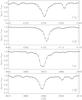 |
Fig. 1 Comparison of our FOCES spectrum (full line) with a longslit spectrum from the NStars project (Gray et al. 2003, dots) in the region of the Balmer lines Hγ to H8 for Deneb (A2 Ia) to assess the quality of the normalisation of our echelle spectra. Note that the FOCES spectrum was was artificially degraded in resolution to match the 1.8 Å resolution of the longslit data. |
A semi-automatic pipeline was used for the reduction of the FOCES data (Pfeiffer et al. 1998), performing subtraction of bias and dark current, flatfielding, wavelength calibration, rectification and merging of echelle orders. As the FOCES observations were obtained over several nights in different years, the conditions and quality varied for each set of exposures. Before the data reduction procedure a median filter was applied to the raw data to remove cosmic ray hits without losing spectral information. Special attention had to be paid to the merging of orders, because key features like the hydrogen lines extend over adjacent orders and their analysis is sensitive to line shape. Moreover, meticulous normalisation procedures were applied (within the reduction pipeline), since imprecise continuum determination may lead to incorrect abundance and parameter determination. Comparison of our data with longslit spectra of fundamental MK standards obtained within the NStars project2 (Gray et al. 2003) was possible for some cases and showed good agreement. Figure 1 exemplifies such a comparison of a NStars project 1.8 Å-resolution spectrum around the Balmer lines Hγ to H8 of Deneb (taken at the Dark Sky Observatory) with our FOCES spectrum, which was artificially degraded in resolution to match that of the NStars project spectrum. Finally, for several objects multiple exposures were taken and combined to enhance the quality and filter out artifacts.
Additional objects were observed in 2007 at the European Southern Observatory on La Silla, using FEROS (Fiber-fed Extended Range Optical Spectrograph, Kaufer et al. 1999) on the 2.2 m telescope. The spectra cover the wavelength range from ~3600 to 9200 Å at R ≈ 48 000. The raw spectra were mainly processed by the ESO automatic reduction pipeline. In addition to spectra of our science targets, a template spectrum of a subdwarf B star was obtained and reduced with the pipeline. By dividing this spectrum through a well-fitting model we could successfully filter out all artifacts from the data reduction process, providing – after proper smoothing to remove localised noise relics – a template function for the continuum rectification of the science target spectra. This procedure provides an objective and reproducible means for the normalisation process.
Additional high-quality spectra of bright BA-type supergiants were extracted from the database of the UVES Paranal Observatory Project (Bagnulo et al. 2003). These data combine a high resolution of R ≈ 80 000 and high S/N with large wavelength coverage from 3040 to 10 400 Å, completing our sample.
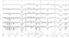 |
Fig. 2 Normalised spectra of an Teff-sequence of sample stars around Hγ (left), Hα (middle) and Pa13 (right panel), from the hot (top) to the cool end of the parameter range investigated here (bottom). The major spectral features are identified, short vertical marks indicate Ti ii lines. The Hα region is contaminated by narrow telluric lines. Vertical shifts of the spectra by multiples of 0.5 have been applied for clarity. |
All together, this comprises the most comprehensive sample of Galactic BA-type supergiants3 with high-quality spectra considered for quantitative analysis to date.
The high-quality spectra allow a much closer look to be taken on trends in spectral line strengths and line ratios than possible with traditional classification spectra at much lower resolution. We used the opportunity to reassess the spectral classification of the sample stars. Starting point of our approach were the anchor points of the MK system (as identified in Table 1), supplemented by MK primary standards as given by Johnson & Morgan (1953), see also Table 1. These cover about half of our sample stars. Spectral types for the remaining stars were assessed on basis of the helium and metal lines, luminosity classes by the width of the Balmer lines. In general, good agreement with the classification as obtained from SIMBAD was found. Maximum changes indicated by our inspection, for about half of the non-MK stars, amount to one spectral subtype or to one subtype (higher or lower) within the supergiant luminosity class. Our reclassification is indicated in Table 1. We note that two of the primary MK standards (HD 14489 and HD 223960) were found to differ significantly in spectral morphology from the stars of similar original spectral type. Also the luminosity appears overestimated for HD 212593, which shows a nearly symmetric Hα absorption profile. We therefore propose a (slight) reclassification for these stars as well, based on the available high-resolution spectra.
Spectra of several sample stars are displayed in Fig. 2, for three strategic wavelength regions around Hγ, Hα and Pa13. A sequence in spectral type from B8 to A3 is shown, the earliest and latest types observed here. Note the rapid strengthening of the metal lines towards lower effective temperatures, and their enormous increase in number. The spectra were shifted to the laboratory rest frame and the major spectral features are identified, many of which were analysed in our project.
Not unexpected are the asymmetric Hα line profiles, indicating the presence of a stellar wind of varying strength in the different stars. P-Cygni-like profiles like in β Ori are an exception, occurring only in the highest-luminosity objects (being most extreme in HD 12953). Typical for many stars of the sample is excess emission in the red wing of Hα like for the A0-A3 stars in Fig. 2. Only the luminosity class Ib stars show Hα completely in absorption, with only small asymmetries being present. See the atlas of Verdugo et al. (1999a) for more examples on A-type supergiant spectra.
In addition to the spectra, which constitute the principal data for the analysis, various (spectro-)photometric data were adopted from the literature for constructing spectral energy distributions. Johnson UBV-magnitudes were taken from Mermilliod & Mermilliod (1994) (see Table 1), which are means of previously published photoelectric data, and JHK-magnitudes from the Two Micron All Sky Survey (Cutri et al. 2003; Skrutskie et al. 2006, 2MASS). Additionally, flux-calibrated, low-dispersion spectra observed with the International Ultraviolet Explorer (IUE) were extracted from the MAST archive4, where available (i.e. for 16 objects). For seven objects only high-resolution IUE spectra are present in the MAST archive, which are nevertheless useful for our purposes as they were observed using a large aperture (i.e. flux-losses should have not occured). These data cover the range from 1150 to 1980 Å for the short (SW) and from 1850 to 3290 Å for the long wavelength (LW) range camera. Typically, both wavelength ranges were observed the same day. A summary of the individual spectra used in the present work (data ID number and observation date) is given in Table 2. Finally, photometric data in the Strömgren system was adopted from the catalog of Hauck & Mermilliod (1998, not tabulated here).
IUE spectra used in this study.
3. Quantitative analysis
3.1. Models and analysis methodology
Advanced models and robust analysis techniques are required in order to achieve the targeted accuracy and precision in stellar parameter and abundance determination. A suitable analysis methodology was presented by Przybilla et al. (2006), which we adopted for the present work, with some extensions as summarised below. The method is based on a hybrid non-LTE approach, in which non-LTE line-formation computations are performed on top of LTE model atmospheres5.
In brief, LTE model atmospheres were computed using the Atlas9 code (Kurucz 1993a) with some additional modifications necessary to allow model convergence close to the Eddington limit (Przybilla et al. 2001b). Line blanketing was accounted for via Kurucz’ Opacity Distribution Functions (Kurucz 1993b). Based on these model atmospheres the non-LTE calculations were performed with recent versions of Detail and Surface (Giddings 1981; Butler & Giddings 1985, both updated by Butler). The coupled radiative transfer and statistical equilibrium equations were solved with Detail, providing non-LTE level populations. Subsequently, synthetic spectra were computed with Surface, using refined line-broadening theories. State-of-the-art model atoms according to Table 3 were adopted for the calculation of the model grids.
Model atoms for non-LTE calculations.
Overall, around 25 000 model spectra per element were combined into 5-dimensional grids. The parameter space covered ranges from 8300 K to 15 500 K in effective temperature Teff (in steps of 250−500 K), from 2.50 in surface gravity log g (cgs units) to the convergence limit at 0.95 (lower Teff-limit) to 1.90 (upper Teff-limit, in steps of 0.1 dex), from 3 km s-1 to 8 km s-1 in microturbulence ξ (1 km s-1 steps) and from 0.09 to 0.15 in helium abundance (by number, steps of 0.015). Finally, sufficient coverage in elemental abundance (typically 1 dex in steps of 0.25 dex) for the respective lines investigated is provided.
Models of Doppler-shift profiles were computed by disk integration, using the methods described in Gray (2005). We divided the apparent disk of a star in 16 million parts of equal size. For each disk position, the radial-tangential velocity distribution, representing macroturbulence6, was projected on the line of sight, assuming an equal amount of radial and tangential motion. The result was then Doppler-shifted according to stellar rotation. Finally, we applied a linear limb-darkening law to determine the weighting factors for integration. The resulting profiles are characterised by three parameters: the projected rotational velocity vsini, the macroturbulent velocity ζ, and the limb-darkening coefficient ϵ.
Theoretical and observed line profiles were compared via the software package Spas (Spectral Plotting and Analysis Suite, Hirsch 2009). It provides the means to interpolate between model grid points for up to three parameters simultaneously and allows to apply instrumental and macrobroadening functions to the resulting theoretical profiles. Furthermore, the program uses the downhill simplex algorithm to minimise χ2 in order to find a good fit to the observed spectrum.
3.2. Spectroscopic indicators
In order to find a globally satisfying solution, it was necessary to derive the basic atmospheric parameters Teff, log g, ξ and y in an iterative process, utilising different spectral indicators on the way. Here we discuss the individual steps of this procedure.
3.2.1. Effective temperature and surface gravity
The hydrogen lines and the ionization equilibria of the metals react sensitive to variations of effective temperature and surface gravity. This dependency was demonstrated for the Stark-broadened hydrogen Balmer lines as well as for e.g. the Mg i/ii lines by Przybilla et al. (2006) and Schiller & Przybilla (2008). While neither the hydrogen lines nor a single ionization equilibrium alone are sufficient to constrain Teff and log g unambiguously due to a degeneracy in the solutions, a combination of at least two of them is, for constant ξ and y. Note that in the low-temperature regime of our sample, where N ii lines are too weak to be analysed, the C i/ii ionization equilibrium is often available to confirm the results obtained from the Mg i/ii lines, while in the high-temperature regime O i/ii becomes available in addition to N i/ii. For the majority of the stars two or in some cases even three metal ionization equilibria can thus be utilised for the atmospheric parameter determination. Hα (see Fig. 2) and, in the most luminous objects, even Hβ and Hγ can be affected by the presence of a significant stellar wind. Consequently, these lines have to be omitted in such cases for the derivation of basic atmospheric parameters in our hydrostatic approach. Hβ and Hγ are therefore considered for most stars, and several of the higher Balmer lines are analysed in all stars, with the exact number depending on the wavelength coverage of the spectrograph, and the S/N reached in the blue orders. If ionization equilibria for more than one element are available for analysis, the results show typically high consistency. An example for the agreement of a final solution with observation is shown in Fig. 3.
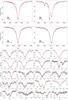 |
Fig. 3 Example for a set of diagnostic lines used in the determination of the atmospheric parameters Teff and log g in the supergiant HD 106068 (B8 Iab), consisting of hydrogen, nitrogen and oxygen lines. The models calculated for our final parameters (red lines) are compared to observation (black lines). The same values of oxygen and nitrogen abundance are adopted for all lines, regardless of ionization stage. The ionization equilibria and the Balmer lines unaffected by the stellar wind are reproduced simultaneously. Note that various line blends of stellar, interstellar and terrestrial nature seen in the plots are exempted from the fitting process. |
3.2.2. Microturbulence and helium abundance
The microturbulent velocity is usually determined by demanding that the abundances indicated by the lines within an ion are independent of equivalent width. This is basically equivalent to finding the microturbulence value that minimises the line-to-line scatter in abundance, which is our preferred method (as we use line-profile fits for this like for the rest of the analysis). Within the framework of the present paper the nitrogen spectra are the most useful indicators for microturbulence as they provide many lines of widely differing strength, while e.g. the more extensive Fe ii line analysis (to be discussed in Paper III), among others, can be used to verify the ξ-determination. An example is shown in Fig. 4, using the traditional form of illustration. Equivalent widths were determined using direct integration over the line profile. Linear regression curves to the data points are consistent with a slope of zero in both cases. A single value for ξ was found to be consistent for all elements analysed in non-LTE in the individual stars, see Fig. 13 of Przybilla et al. (2006) for a comprehensive discussion in the case of HD 87737. Note that while the Balmer-lines are virtually insensitive to microturbulence variations, this quantity influences the parameter determination based on ionization equilibria.
A change in the atmospheric helium abundance gives rise to a modified mean molecular weight of the atmospheric plasma, which has similar effects on model predictions than a variation of log g (Kudritzki 1973; Przybilla et al. 2006). Therefore, the helium abundance y has to be constrained simultaneously with the other atmospheric parameters. This is done via line-profile fitting of helium lines. Results for the individual He i line abundances in the sample stars can be found in Paper II.
In practice, estimates for ξ and y are used to determine initial values for Teff and log g in a first iteration step (using elemental abundances as third fit parameter), which are in turn adopted to derive ξ and y in a next step. Convergence is quickly achieved using our comprehensive model grids and Spas.
3.2.3. Projected rotational velocity and macroturbulence
In order to perform line-profile-fitting it is necessary that the models are able to reproduce the line-shapes accurately. To achieve this our model spectra are convolved with the functions for rotational and macroturbulent broadening computed as described earlier. A value of 0.5 for the limb-darkening coefficient ϵ was adopted throughout. Tests showed little sensitivity for this parameter within acceptable bounds, which is only slowly varying around our canonical value throughout the atmospheric parameter and spectral wavelength range investigated here (see e.g. Wade & Rucinski 1985).
We chose the same set of highly suitable metal lines to derive vsini and ζ in most of our targets, including the Mg ii line at 4390 Å, the Mg i line at 5183 Å, the Fe ii pair around 6148 Å, and the O i triplet around 6157 Å. However, for the two hottest objects in our sample only the S ii line at 5354 Å was used. Examples from the fitting are shown in the upper panels of Fig. 5, displaying a goodness-of-fit parameter in (vsini, ζ) space. While in theory this should allow us to identify the optimum values for vsini and ζ, we found disentanglement of the effects from rotational velocity and macroturbulence to be difficult because of the rather smeared contours. This is similar to other recent studies of rotational broadening in BA-type supergiants (Verdugo et al. 1999b; Ryans et al. 2002). Values of vsini and ζ representing the best fits show a scatter from line to line because of this degeneracy in the solutions. Fits without macroturbulence contribution agree very well in the resulting vsini for different absorption features. However, they can not reproduce observations in such a satisfactory way like fits that consider both effects, see the lower panels of Fig. 5 for a comparison. Overall, the uncertainties of vsini and ζ are typically about ±5 km s-1 because of the degeneracy of the solutions, and about ±3 km s-1 for the stars with the sharpest lines.
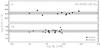 |
Fig. 4 Abundance values derived from single lines are presented versus respective equivalent widths for a selection of lines from neutral and ionized nitrogen and iron in the spectrum of HD 46300 (A0 Ib). The 1σ-scatter around the mean value is indicated by the gray bands. |
3.2.4. Abundances and metallicity
Abundances for all ionization stages involved in the atmospheric parameter determination were derived, as summarised in Table 4. For this, the individual lines of an ion were fitted and the mean of the resulting abundances was taken. For the sake of brevity we postpone a presentation of individual line abundances for the sample stars to Papers II and III, where the complete data will be discussed, irrespective of the availability of ionization equilibria.
Overall, good to excellent agreement between different ionization stages of the elements was found, even in cases where more than one ionization equilibrium was evaluated, indicating that major bias is likely absent in our atmospheric parameter determination. The statistical uncertainties arising from noise prove to be small due to the high quality of our spectra. Only for the weakest lines used in our analysis they are comparable to the line-to-line scatter. Therefore we chose the 1σ standard deviation based on the individual line abundances as a conservative error estimate for the ion abundances. In this approach it is difficult to assign an uncertainty value for an ion where only one line is available for analysis. An inspection of the data in Table 4 indicates that a characteristic estimate in such a case may be 0.10 dex.
Low star-to-star scatter in metallicity was found in recent analyses of early B-type dwarfs – the progenitors of BA-type supergiants on the main sequence – in the solar neighbourhood (Przybilla et al. 2008; Nieva & Simón-Díaz 2011; Nieva & Przybilla 2012), using similar analysis techniques. Given the low sensitivity of our analysis to small changes in metallicity (Przybilla et al. 2006), this parameter was held fixed throughout our model grid to slightly subsolar values (with respect to the solar standard of Grevesse & Sauval 1998) in accordance with the B-dwarf results (the cosmic abundance standard). This approximation was proved correct a-posteriori by our abundance analysis for most of the sample stars. We reanalysed the most metal-rich stars of our sample later on by means of fine-tuned micro-grids, adopting a higher value for the metallicity in order to rule out any possible bias due to this.
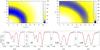 |
Fig. 5 Examples for the derivation of vsini and ζ from the O i triplet around 6157 Å (left) in HD 207673 and the Fe ii pair around 6148 Å (right) in HD 14433. The upper panels show contour plots of a goodness-of-fit parameter in (vsini, ζ) space, lower values representing a better fit. The lower panels display the best line-profile-fits with and without macroturbulence (left and right, respectively). |
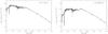 |
Fig. 6 Examples of comparisons of Atlas9 model fluxes (black lines) with UV-spectrophotometry from the IUE satellite (gray lines) and with photometric measurements – UBV from Mermilliod & Mermilliod (1994), JHK from 2MASS – for two of our sample stars. The SEDs shown are dereddened according to the values of E(B − V) and RV in Table 4, and normalised in V. |
3.2.5. Spectral energy distribution
As a verification of our spectroscopic analysis we compared the Atlas9 fluxes computed for our final parameters with photometric data in the optical and near-IR, and UV spectrophotometry. Thus, we investigated whether the models reproduce also the spectral energy distributions (SEDs) of the stars, and as a consequence also their global energy output.
We transformed the UBV and JHK magnitudes into absolute fluxes using zeropoints from Bessell et al. (1998) for Johnson photometry and from Cohen et al. (2003) for the 2MASS photometric system. Note that we lowered the U photometric zero point by 3% based on discrepancies between theory and observation that were found by Bohlin & Gilliland (2004) in the respective part of the UV-flux for the photometric standard star Vega.
The observed fluxes needed to be dereddened for the comparison with the model fluxes. For this, we adopted the mean interstellar extinction law of Cardelli et al. (1989), which is depending on one parameter, the ratio of total-to-selective extinction RV = AV/E(B − V). The colour excess E(B − V) was determined per star as the difference between the theoretical colour computed from the Atlas9 flux and the observed colour. Then, RV was varied until a good overall match of the theoretical and the observed SED was achieved, see Fig. 6 for examples of final results. The typical uncertainty in RV is ±0.2. This could be done also for the twelve stars without IUE spectrophotometry, though lacking the very thorough constraints by the UV fluxes.
In general, as good agreement between the model and the observed SED is found as exemplified in Fig. 6. Notable deviations occur only in three cases. An IR excess is found for HD 21291, while the UV-flux is in excellent agreement. We attribute this to HD 21291 being part of a close visual binary separated by only 2.39″ (Prieur et al. 2008), which could not be resolved by 2MASS. An UV excess in HD 187983 can be explained by adding flux from an early B-type main-sequence companion, which is consistent with a radial-velocity variation found by Hendry (1981). There remain some problems in reproducing the SED of HD 12953, the most luminous object in our sample, similar to those found for HD 92207 (A0 Iae) by Przybilla et al. (2006). Further investigations are required to address the issue, but these are beyond the scope of the present work.
Finally, a by-product of our investigations are bolometric corrections B.C. for the sample stars. They were derived from the fluxes of our final models, see Sect. 5.4 for a discussion.
4. Results
4.1. Atmospheric parameters of the sample stars
Our results on the atmospheric parameters and some derived properties of the sample stars are summarised in Table 4. For each object our internal sequential number and its HD-designation are given, followed by our determinations of effective temperature, surface gravity, microturbulent, projected rotational and macroturbulent velocity, colour excess, ratio of total-to-selective extinction and bolometric correction. Finally, surface abundances of helium and – for the cases where the respective ionization equilibria were employed for the atmospheric parameter determination – abundances of metal ions are summarised. The error margins denote 1σ-uncertainties (an estimate of 0.10 dex may be applied for ion abundances where only one line could be analysed, i.e. those data without uncertainty indicator). Uncertainies in vsini and ζ amount typically to ±5 km s-1 (±3 km s-1 for the stars with the sharpest lines) because of the degeneracy of the solution in the fitting of vsini and ζ, see Sect. 3.2.3, and ±0.2 in RV, see Sect. 3.2.5. The uncertainties of the bolometric corrections vary from ~0.02 mag for the coolest sample stars to ~0.05 mag for the hottest stars, see Sect. 5.4 for a more detailed discussion. This is the most comprehensive collection of such data from a homogeneous non-LTE analysis of Galactic BA-type supergiants to date. As expected, a continuous distribution over the temperature range from 8400 to 12 700 K is obtained, displaying no signs of systematic shifts or gaps stemming from the use of different temperature indicators.
Stellar parameters of the program stars.
Tests with a bootstrapping method implemented in Spas indicate formal uncertainties of less than 0.05 dex in log g and 1% in Teff, when all other parameters are held constant at the values of our final solution. This applies even for the lowest-quality spectra of our sample (at S/N of about 120). Fits to individual Balmer lines – the main indicators for log g throughout the sample – show a scatter of less than 0.05 dex around the mean value in this parameter in the individual stars. This suggests that major systematic effects from order merging and normalisation in the hydrogen lines may be absent.
The line-to-line scatter in abundances derived from individual metal lines, however, indicates low-level systematic uncertainties from within our model atoms and the normalisation of weak lines. Small selection effects may also emerge in cases where only a few lines in one ion of the two analysed for establishing ionization balance are available. Therefore, when line sets of sufficient quality for two or more elements were available, we compared different solutions using only one of the available ionization equilibria and the Balmer lines. While still showing good agreement, the results imply slightly higher uncertainties than discussed earlier. Hence we chose our uncertainty estimates carefully across the parameter space, remaining conservative in the values given in Table 4. The largest discrepancies were found for the case when the last residual Mg i lines (Mg i λ5183 Å being the strongest) are about to vanish. In consequence, the largest uncertainties occur in the transition region when N i/ii starts to replace the Mg i/ii-balance. Overall, the typical conservative uncertainties in Teff and log g are therefore ~2% (150−200 K) and 0.10 dex (i.e. ~25% in gravity), respectively, accounting for both statistical and systematic errors.
Our accuracy in microturbulence determination is limited by the stepsize of 1 km s-1 in our model grid. The values derived from different elemental species are consistent within this error. The derived helium abundances vary between 10 and 14% in number fraction, with errors of around 20% in these values. Note, however, that the high sensitivity of the helium lines to Teff-variations makes the values prone to substantial systematic shifts even from small errors in the parameter determination. Finally, metal abundances are determined on average with about 10−20% uncertainty. Abundances from lines of the major ionization stages are usually insensitive to variations of Teff and log g within the given uncertainties.
4.2. Comparison with previous analyses
Samples of about 10−20 Galactic supergiants in the BA-star regime were subject to non-LTE analyses in three previous studies (Venn 1995a; McErlean et al. 1999; Takeda & Takada-Hidai 2000). We list their effective temperatures and surface gravities for stars in common with the present work in Table 5. Typical uncertainties in Teff/log g are 200 K/0.2 dex, 500−1000 K/0.5 dex and 1000 K/0.2 dex in these studies, respectively.
Venn (1995a) used a similar method for the parameter determination in A-type supergiants, i.e., utilising the Balmer- and Mg i/ii-lines, however without a simultaneous derivation of the He abundance in her hybrid non-LTE approach. While there are some differences, good overall agreement is found in Teff and log g within the uncertainties.
Takeda & Takada-Hidai (2000) tried to construct a Teff/log g vs. spectral type relation, utilising published data. They emphasised, however, that this approach is subject to considerable uncertainties. Indeed, we find notable deviations between our values for both Teff and log g and their data, though agreement is still found when considering their rather large uncertainty ranges.
Finally, there is some overlap with the B-type supergiants studied by McErlean et al. (1999). Their estimates for log g, inferred from the Balmer lines, are in excellent agreement with ours. Yet, we find a systematic shift in Teff towards higher values compared to our results. Their temperatures are based on the non-LTE Si ii/iii ionization balance for the stars in common (except for HD 21291, where photometry was used as substitute). However, the non-LTE model atmospheres used for their analysis did not consider the effects of metal line-blanketing, which we identify as the likely cause of the Teff-differences.
5. First applications
5.1. Spectral type–Teff relation
Empirical spectral-type–Teff relations provide important starting points for all kinds of stellar studies and for quantitative spectroscopy in particular, and they are therefore an essential part of the reference literature on stellar properties. Our high-precision/high-accuracy dataset facilitates to reassess the existing knowledge in the BA-type supergiant regime in view of improved models and analysis techniques.
Comparison of our atmospheric parameters (Teff [K], log g) for objects in common with previous studies.
Spectral type–Teff–(B − V)0–(b − y)0 scales & B.C. values for Galactic BA-type supergiants.
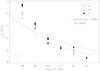 |
Fig. 7 Comparison of our results for the individual sample stars with reference spectral type–Teff scales. Luminosity classes and reference scales are encoded according to the legend. A typical error bar is indicated to the lower left. See Sect. 5.1 for a discussion. |
Effective temperatures of our sample stars (see Table 4) as a function of their spectral type (according to the refined classification presented in Table 1) are displayed in Fig. 7. In comparison with established reference work (Schmidt-Kaler 1982; Cox 2000) we find a significantly steeper spectral-type–Teff relation, i.e. higher Teff at spectral types B8 and B9, and lower Teff at A2 and A3. As no apparent correlation of Teff with luminosity class (LC) is indicated in Fig. 7, we compute average Teff-values from all stars of a spectral subtype to provide refined reference values which are presented in Table 6.
With typically five to seven objects per spectral type it would be desirable to increase the sample size in order to get a more robust determination, in particular of the uncertainties. The distribution of the data per spectral bin is not Gaussian at the moment. Note that the formal 1σ-uncertainties for spectral types A1 and A3 in Table 6 are lower than the uncertainties from the individual star analyses. There is little overlap of Teff-values for individual stars of different spectral types. Overall it appears that our refined spectral-type–Teff relation allows effective temperatures to be estimated with a typical 1σ-uncertainty of about 2−3%.
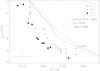 |
Fig. 8 Comparison of observational results for the individual sample stars with established reference (B − V)0–Teff relations from the literature, according to the legend. A typical error bar is indicated. See Sect. 5.2 for a discussion. |
Obviously, the work has to be extended in the future to provide a unified picture accounting for recent developments concerning hotter (e.g. Repolust et al. 2004; Markova & Puls 2008) and cooler Galactic supergiants (e.g. Levesque et al. 2005).
5.2. (B – V)0–Teff scale
Closely related to the spectral-type–Teff relation is the question of the behaviour of intrinsic Johnson colour (B − V)0 with spectral type, or more precisely, with effective temperature. We determined (B − V)0 from the observed (B − V) colour (see Table 1), corrected for the colour excess E(B − V) according to Table 4.
Our effective temperatures as a function
of (B − V)0 are displayed in Fig. 8, together with established reference relations from
Schmidt-Kaler (1982, for LC Iab), Flower (1996, LC I) and Cox (2000, LC I). Our data are systematically bluer
by  than indicated by the reference
relationships. The supergiants become bluer with decreasing luminosity (i.e. smaller
radius) for a given Teff, the decrement being
about
than indicated by the reference
relationships. The supergiants become bluer with decreasing luminosity (i.e. smaller
radius) for a given Teff, the decrement being
about  per luminosity subclass. As we do not have
enough objects per spectral type to compute meaningful means for the individual luminosity
subclasses, we provide (B − V)0-values
averaged over the entire LC I in Table 6. Note that
the outlier HD 12953 – the by far the most luminous star of our sample – has been
excluded from this.
per luminosity subclass. As we do not have
enough objects per spectral type to compute meaningful means for the individual luminosity
subclasses, we provide (B − V)0-values
averaged over the entire LC I in Table 6. Note that
the outlier HD 12953 – the by far the most luminous star of our sample – has been
excluded from this.
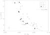 |
Fig. 9 Comparison of observational results for the sample stars with a reference (b − y)0–Teff relation from the literature, according to the legend. A typical error bar is indicated. See Sect. 5.3 for a discussion. |
The loci of the three luminosity subclasses of BA-type supergiants in Fig. 8 may be approximated by a quadratic fit function,
yielding the following relations 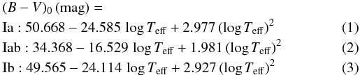 with an area of validity of about
3.92 ≲ log Teff ≲ 4.10. Like for the case of the spectral
type–Teff relation it would be desirable to extend this to
hotter and cooler supergiants.
with an area of validity of about
3.92 ≲ log Teff ≲ 4.10. Like for the case of the spectral
type–Teff relation it would be desirable to extend this to
hotter and cooler supergiants.
5.3. (b – y)0–Teff scale
Our effective temperatures as a function of
Strömgren (b − y)0 are displayed in
Fig. 9, together with a reference relation from
Gray (1992, for LC Ib). There is an excellent
match of Gray’s relation with our data. Note the drastic change of the slope of the
(b − y)0–Teff-relation
for bluer (b − y)0. In general,
the supergiants become bluer with decreasing luminosity for a
given Teff, the decrement being about
per luminosity subclass. Like for the
previous case of the Johnson data, we provide
(b − y)0-values averaged over the entire
LC I in Table 6. The outlier HD 12953, which
appears exceptionally blue
in (b − y)0, has been excluded.
The loci of the three luminosity subclasses of BA-type supergiants in Fig. 9 may be approximated by a quadratic fit function,
yielding the following relations 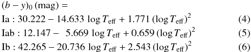 with an area of validity of about
3.92 ≲ log Teff ≲ 4.10.
with an area of validity of about
3.92 ≲ log Teff ≲ 4.10.
5.4. Bolometric corrections
We determined bolometric corrections from the model fluxes for each individual star.
Following the approach of Bessell et al. (1998), the
model flux at the V-band effective wavelength was
converted into a Johnson V magnitude in the usual way by adopting a
zeropoint flux  = 3.636 × 10⁻²⁰ erg cm-2 s-1 Hz-1
(for Vega). The integral over the total model spectral energy distribution yielded a
bolometric magnitude (assuming an absolute solar bolometric magnitude
= 3.636 × 10⁻²⁰ erg cm-2 s-1 Hz-1
(for Vega). The integral over the total model spectral energy distribution yielded a
bolometric magnitude (assuming an absolute solar bolometric magnitude
 = + 4.74). The difference between the
bolometric and the V magnitudes calculated in this way then provided the
bolometric correction, which can be expressed as
= + 4.74). The difference between the
bolometric and the V magnitudes calculated in this way then provided the
bolometric correction, which can be expressed as  (7)where C = 12.854 for a solar
radius R⊙ = 6.95 × 1010 cm and
(7)where C = 12.854 for a solar
radius R⊙ = 6.95 × 1010 cm and
 = 5777 K,
and Hν is the Eddington flux at the
effective V-band frequency. This way, the correct
empirical B.C. for
the standard star Vega is reproduced, which lies exactly in the
Teff-range spanned by the sample stars. Note that for this
reason we have not renormalised the bolometric corrections to the minimum value of zero in
order to avoid positive
B.C.-values for some
late-A and F-type stars, as suggested by Buser & Kurucz
(1978), see also the discussion of this topic by Bessell et al. (1998) and Torres (2010).
As a result, our
B.C. values are
about
= 5777 K,
and Hν is the Eddington flux at the
effective V-band frequency. This way, the correct
empirical B.C. for
the standard star Vega is reproduced, which lies exactly in the
Teff-range spanned by the sample stars. Note that for this
reason we have not renormalised the bolometric corrections to the minimum value of zero in
order to avoid positive
B.C.-values for some
late-A and F-type stars, as suggested by Buser & Kurucz
(1978), see also the discussion of this topic by Bessell et al. (1998) and Torres (2010).
As a result, our
B.C. values are
about  larger than the ones provided earlier by
us when introducing the modelling techniques and analysis methodology used here (Przybilla et al. 2006). The
B.C.-values
determined from Eq. (7), summarised in
Table 4, deviate less
than
larger than the ones provided earlier by
us when introducing the modelling techniques and analysis methodology used here (Przybilla et al. 2006). The
B.C.-values
determined from Eq. (7), summarised in
Table 4, deviate less
than  from the recent analytical fit formula of
Kudritzki et al. (2008b, their Eq. (6)), which
have used the same approach. The uncertainties of the bolometric corrections are dominated
by the Teff-errors. For the coolest sample stars, i.e. close
to the minimum of the
Teff–B.C.-curve,
the uncertainties for individual objects amount to ~0.02 mag, while they reach up
to ~0.05 mag for maximum Teff-uncertainties in the
hottest stars.
from the recent analytical fit formula of
Kudritzki et al. (2008b, their Eq. (6)), which
have used the same approach. The uncertainties of the bolometric corrections are dominated
by the Teff-errors. For the coolest sample stars, i.e. close
to the minimum of the
Teff–B.C.-curve,
the uncertainties for individual objects amount to ~0.02 mag, while they reach up
to ~0.05 mag for maximum Teff-uncertainties in the
hottest stars.
The derived values are compared to the reference calibrations of Schmidt-Kaler (1982, for stars of luminosity class Iab), which are
reproduced by Cox (2000), and of Flower (1996, for supergiants, his Table 4 in Fig. 10.
In order to adjust for the different zeropoints used, we correct the data of
Schmidt-Kaler/Cox by 7.
The resulting differences can reach values up to  . A general trend towards larger
B.C.-values is seen
in our data, except for the hottest objects in the sample, which have slightly lower
bolometric corrections. The match of the Flower relation (adjusted
by
. A general trend towards larger
B.C.-values is seen
in our data, except for the hottest objects in the sample, which have slightly lower
bolometric corrections. The match of the Flower relation (adjusted
by  because of the different zeropoints) on
the other hand is good, with small deviations becoming apparent at the highest and lowest
temperatures considered here.
because of the different zeropoints) on
the other hand is good, with small deviations becoming apparent at the highest and lowest
temperatures considered here.
As no significant deviations occur due to luminosity classification, except possibly for our most luminous sample star HD 12953, we average over all members of a spectral subtype to determine improved B.C. reference values. Our values are compared to the reference data from the literature in Table 6.
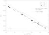 |
Fig. 10 Comparison of bolometric corrections determined here with reference relations from the literature, according to the legend. The error bar denotes a typical uncertainty in Teff and a maximum uncertainty in B.C.. See Sect. 5.4 for a discussion. |
5.5. Photometric atmospheric parameter determination
As one often wishes to analyse larger samples of stars, easy-to-apply and fast stellar parameter indicators are in high demand. Photometric Teff-indicators are among the preferred ones, because of the easy accessibility of photometric data. We discuss empirical relations for the two most common photometric systems, for Johnson and for Strömgren photometry. The latter also allows surface gravities to be estimated photometrically.
The reddening-free Johnson Q-index as Teff-indicator.
Effective temperature calibrations based on the reddening-free Q-index (Johnson 1958), Q = (U − B) − X(B − V) with X = E(U − B)/E(B − V), have come into wide use recently, as Johnson photometry is available for most stars. Examples in our context encompass studies of the evolutionary progenitors of BA-type supergiants, OB-type stars on the main sequence (e.g. Daflon et al. 1999; Lyubimkov et al. 2002), and their cooler siblings, late-A to G-type supergiants (Lyubimkov et al. 2010). Usually, a standard value of 0.72 is adopted for X, but see Johnson (1958).
We test the applicability of the Q-index as possible Teff-indicator for BA-type supergiants in Fig. 11. Our spectroscopically derived Teff-values are displayed as a function of Q. A trend with luminosity subclass becomes apparent, the more luminous Ia objects being coolest and the Ib objects being hottest at a given Q. The loci of the three luminosity subclasses in the diagram may be approximated by a quadratic fit function, yielding the following relations
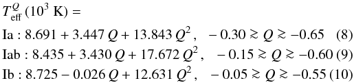 with their respective area of validity. The
outlier HD 12953 was excluded from the fitting procedure. For clarity, only the fit
function for Iab supergiants is visualised in Fig. 11. At first glance, rather tight relations are found.
with their respective area of validity. The
outlier HD 12953 was excluded from the fitting procedure. For clarity, only the fit
function for Iab supergiants is visualised in Fig. 11. At first glance, rather tight relations are found.
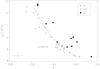 |
Fig. 11 Relation between the reddening-free Johnson Q-index, Q = (U − B) − 0.72(B − V), and the spectroscopic Teff-values of the sample stars. A typical error bar is indicated. The dashed line represents the regression line of our Q-based Teff-calibration for Iab supergiants. |
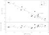 |
Fig. 12 Upper panel: comparison of our spectroscopically derived
|
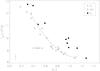 |
Fig. 13 As Fig. 11, but for the relation between the reddening-free Strömgren [c1] -index, [c1] = c1 − 0.20(b − y) where c1 = (u − v) − (v − b)), and the spectroscopic Teff-values of the sample stars. |
The differences between the spectroscopically derived effective
temperatures  and the Q-based
 computed with Eqs. (8)−(10) are quantified in Fig. 12. The
sample stars follow the 1:1 relation rather tightly, with the
1σ-scatter of the computed around the spectroscopic reference
values amounting to more than 3%. This is the systematic uncertainty
adherent to an application of the method. In addition, random errors
because of the uncertainties in the colours also have to be considered,
typically amounting to more than twice the 1σ-uncertainty of the
spectroscopically derived values, i.e. another ~5% (see the error bar in the upper
panel of Fig. 12 and note the different scale
projection of the axes). In consequence, the resulting error margins render this
simple approach of Q-based effective temperatures
not competitive with spectroscopic determinations for BA-type supergiants.
Moreover, better starting points for an iterative refinement of the stellar parameters
are already obtained from the spectral type–Teff relation
established in Sect. 5.1.
computed with Eqs. (8)−(10) are quantified in Fig. 12. The
sample stars follow the 1:1 relation rather tightly, with the
1σ-scatter of the computed around the spectroscopic reference
values amounting to more than 3%. This is the systematic uncertainty
adherent to an application of the method. In addition, random errors
because of the uncertainties in the colours also have to be considered,
typically amounting to more than twice the 1σ-uncertainty of the
spectroscopically derived values, i.e. another ~5% (see the error bar in the upper
panel of Fig. 12 and note the different scale
projection of the axes). In consequence, the resulting error margins render this
simple approach of Q-based effective temperatures
not competitive with spectroscopic determinations for BA-type supergiants.
Moreover, better starting points for an iterative refinement of the stellar parameters
are already obtained from the spectral type–Teff relation
established in Sect. 5.1.
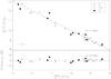 |
Fig. 14 As Fig. 12, but for the comparison of our
spectroscopically derived |
The reddening-free Strömgren [c1]-index as Teff-indicator.
Data for 31 of our sample supergiants were found in the catalogue of Hauck & Mermilliod (1998) on Strömgren
uvbyβ photometry, facilitating the reddening-free
[c1] -index
[c1] = c1 − 0.20(b − y)
to be computed, with
c1 = (u − v) − (v − b).
Figure 13 visualises the sample stars in the
[c1] –Teff plane. The loci of
the three luminosity subclasses may be approximated by a quadratic fit function as
before, yielding the following relations
![Mathematical equation: \begin{eqnarray} && T_{\rm eff}^{[c_1]}\,(10^3\,{\rm K})= \nonumber \\ \label{Iacalstr}&& {\rm Ia:} 14.610-11.706\,[c_1]+5.855\,[c_1]^2\,,0.15\la [c_1]\la0.90\quad\quad \\ \label{Iabcalstr}&& {\rm Iab:} 15.741-12.710\,[c_1]+5.536\,[c_1]^2\,,0.35\la [c_1]\la 1.10\quad\quad \\ \label{Ibcalstr}&& {\rm Ib:} 14.310-~\,5.893\,[c_1]+1.092\,[c_1]^2\,,0.25\la [c_1]\la 1.25\quad\quad \end{eqnarray}](/articles/aa/full_html/2012/07/aa19034-12/aa19034-12-eq89.png) with their respective
area of validity. For clarity, only the fit function for Iab supergiants is visualised
in Fig. 13. The clear outlier HD 12953 was ignored
in the determination of the fit coefficients in Eq. (11). The Strömgren
[c1] –Teff relations are
obviously tighter than the Johnson
Q–Teff relations. In fact, a practical
common relation for BA-type supergiants of luminosity class Ia and Iab
can be given with only a negligible loss in accuracy for the range
0.15 ≲ [c1] ≲ 1.10:
with their respective
area of validity. For clarity, only the fit function for Iab supergiants is visualised
in Fig. 13. The clear outlier HD 12953 was ignored
in the determination of the fit coefficients in Eq. (11). The Strömgren
[c1] –Teff relations are
obviously tighter than the Johnson
Q–Teff relations. In fact, a practical
common relation for BA-type supergiants of luminosity class Ia and Iab
can be given with only a negligible loss in accuracy for the range
0.15 ≲ [c1] ≲ 1.10: ![Mathematical equation: \begin{eqnarray} T_{\rm eff}^{[c_1]}\,(10^3~{\rm K})=14.613-10.565\,[c_1]+4.523\,[c_1]^2. \label{IaIabcalstr} \end{eqnarray}](/articles/aa/full_html/2012/07/aa19034-12/aa19034-12-eq91.png) (14)In analogy to Fig. 12, the differences between and the
[c1] -based
(14)In analogy to Fig. 12, the differences between and the
[c1] -based ![Mathematical equation: \hbox{$T_{\rm eff}^{[c_1]}$}](/articles/aa/full_html/2012/07/aa19034-12/aa19034-12-eq86.png) computed with Eqs. (11)–(13) are quantified in Fig. 14. The
1σ-scatter of the computed around the spectroscopic reference
values amounts to about 2% only in this case (systematic uncertainty of the method). The
random errors due to Strömgren colour uncertainties are also drastically reduced
compared to Johnson photometry, amounting to about 1%. We conclude that the
reddening-free [c1] -index provides
highly useful starting values for Teff in
high-precision/accuracy analyses of all except the most luminous BA-type
supergiants.
computed with Eqs. (11)–(13) are quantified in Fig. 14. The
1σ-scatter of the computed around the spectroscopic reference
values amounts to about 2% only in this case (systematic uncertainty of the method). The
random errors due to Strömgren colour uncertainties are also drastically reduced
compared to Johnson photometry, amounting to about 1%. We conclude that the
reddening-free [c1] -index provides
highly useful starting values for Teff in
high-precision/accuracy analyses of all except the most luminous BA-type
supergiants.
As the reddening-free Strömgren [c1] -index measures the Balmer decrement8 at the temperatures of the sample stars, it could act as a substitute for the Balmer jump method (Kudritzki et al. 2008b) based on flux-calibrated low/intermediate spectroscopy, that has been used for studies of BA-type supergiants in galaxies beyond the Local Group recently. Extended exposures in a spectral region with usually low instrumental sensitivity (decrease of mirror coating reflectivity and CCD sensitivity towards the optical-UV) could thus be avoided. However, practical challenges to be solved first are the determination of the metallicity dependency of the [c1] –Teff relation and the availability of Strömgren filter sets at large telescopes.
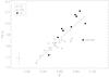 |
Fig. 15 Relation between Strömgren β and the spectroscopically derived flux-weighted gravities log gF of the sample stars. The error bar in β is an estimate based on the restricted information available from the Strömgren data. The dashed line represents the linear regression to the data, ignoring the outlier HD 210221. |
Strömgren β as a photometric gravity indicator.
The Strömgren β-index is a poor direct indicator for
surface gravity in the parameter range of BA-type supergiants because the strength of
the Balmer lines depends not only on log g – pressure broadening via
the linear Stark effect – alone but also on Teff – via
(de-)population of the n = 2 level of neutral hydrogen by
excitation/ionization. On the other hand, there is a good correlation with the
flux-weighted gravity 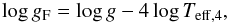 (15)as illustrated by Fig. 15. Here,
Teff,4 = Teff/10 000 K. The
flux-weighted gravity is a measure for the stellar luminosity (Kudritzki et al. 2003, 2008b),
with lower values indicating higher luminosity. Linear regression of the data yields
(15)as illustrated by Fig. 15. Here,
Teff,4 = Teff/10 000 K. The
flux-weighted gravity is a measure for the stellar luminosity (Kudritzki et al. 2003, 2008b),
with lower values indicating higher luminosity. Linear regression of the data yields
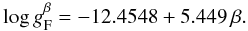 (16)One statistical outlier, HD 210221, was
excluded from the fit based on its distance to the remainder of the data points. The
random 1σ-uncertainty due to errors in the measurements
of β is typically 0.03 dex, and the application of Eq. (16) yields the flux-weighted gravity to
within 0.13 dex (systematic 1σ-uncertainties), see Fig. 16.
(16)One statistical outlier, HD 210221, was
excluded from the fit based on its distance to the remainder of the data points. The
random 1σ-uncertainty due to errors in the measurements
of β is typically 0.03 dex, and the application of Eq. (16) yields the flux-weighted gravity to
within 0.13 dex (systematic 1σ-uncertainties), see Fig. 16.
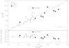 |
Fig. 16 Upper panel: comparison of our spectroscopically
derived |

The conversion of  to the β-based surface
gravity log gβ is facilitated by
correction with the [c1] -based effective temperature,
as established before. The uncertainties of contribute little to the error budget
of log gβ, resulting in error margins
of ±0.04 dex (1σ random) ± 0.13 dex (1σ systematic
uncertainty).
to the β-based surface
gravity log gβ is facilitated by
correction with the [c1] -based effective temperature,
as established before. The uncertainties of contribute little to the error budget
of log gβ, resulting in error margins
of ±0.04 dex (1σ random) ± 0.13 dex (1σ systematic
uncertainty).
In particular the [c1] –Teff (assisted by a determination of the luminosity subclass from spectroscopy) and the β–log gF relations derived here should facilitate to provide useful starting values of Teff and log g for detailed quantitative analyses of normal BA-type supergiants. Exceptions may be the most luminous objects (those with pronounced Hα P-Cygni profiles like HD 12953), which as a class of their own fall out of relations given here.
The photometric starting values must be refined – preferentially through an iterative methodology like the one discussed in Sect. 3 – in the spectroscopic analysis if high accuracy and precision is desired in the derivation of all dependent quantities. The reason for this is illustrated in Fig. 17, which shows both the results of the atmospheric parameter determination from our detailed spectroscopic analysis and from application of the photometric indicators discussed here in the Teff–log g plane. Despite “inconspicuous” error bars (see Fig. 17), the photometric indicators without a subsequent refinement would yield different solutions for the fundamental stellar parameters (mass, radius, luminosity) and for elemental abundances. Symptoms of the presence of such systematics would become evident in any more detailed analysis, as a failure to establish the ionization balance for multiple elements simultaneously, and very likely a mismatch of theoretical and observed profiles for some hydrogen lines. Results biased in such a way can easily lead to misinterpretations and incorrect conclusions in the astrophysical context, see Fig. 5 of Simón-Díaz (2010) for a good example on the effect for the elemental abundance determination, and his discussion of this. In terms of fundamental stellar parameters, we see e.g. that evolutionary masses from the comparison with stellar evolution tracks in Fig. 17 could be biased by up to ~30%.
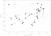 |
Fig. 17 The sample stars with Strömgren photometric data in the Teff–log g plane. Solutions from the spectroscopic determination are shown as dots, open circles mark values that are obtained using photometric indicators according to our calibrations using [c1] and β. The two corresponding solutions are interconnected. Typical error bars are indicated in the upper left. Dotted lines mark evolution tracks for rotating stars at metallicity Z = 0.014 (Ekström et al. 2012), from 9 M⊙ to 32 M⊙ (bottom to top). The 9 M⊙ model shows a blue loop, partially displayed here. |
5.6. Tracers for studies of the ISM
Properties of the interstellar medium (ISM) are usually investigated by using early-type stars as background light sources, facilitating to study absorption and scattering by the intervening interstellar material along the line of sight. While the topic is too broad for the scope of the present paper, we nevertheless want to point out the usefulness of BA-type supergiants for such studies briefly, in particular for the example of the ratio of total-to-selective extinction RV.
Our derived RV-values for the sample stars (see Table 4) cluster around the frequently quoted standard value of RV = 3.1 (e.g. Savage & Mathis 1979), with an rms scatter of 0.3. The data are displayed in Fig. 18, as a function of position in the Galactic plane (Galactic coordinates l and b are used, note that two stars fall outside the displayed range, HD 34085 and HD 87737, which are located at higher Galactic latitude). We find the objects with higher values than RV = 3.1 concentrated in the southern Milky Way around 260° to 360° Galactic longitude, and many objects with lower values in the opposite direction, at l ≈ 60 to 110°. This is in good agreement with previous findings of Whittet (1977).
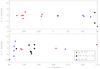 |
Fig. 18 The distribution of our sample supergiants in the Galactic plane, coded according to the legend for values of the total-to-selective extinction ratio RV along the line-of-sight. See Sect. 5.6 for a discussion. |
While our sample is too small to provide any significant extension to modern studies (see e.g. Winkler 1997; Wegner 2003), which consider hundreds of OB stars, we want to draw the attention to the potential of BA-type supergiants for such investigations. Despite their rarity, they are highly useful for probing lines-of-sight towards very distant (or highly reddened) objects in the Milky Way because of their much higher intrinsic visual brightness. Moreover, their usefulness for simple investigations like presented here extends to distances even far beyond the Milky Way (e.g. Kudritzki et al. 2008b, 2012; U et al. 2009). It is reassuring in this context to find the RV-values for many independent Galactic sightlines to cluster close to the canonical value. A ratio of total-to-selective extinction of 3.1 may therefore be a good assumption for many extragalactic environments, where full SED information of individual stars, required for the determination of RV, is unavailable at present.
In addition, luminous BA-type supergiants facilitate also more sophisticated studies of the ISM in other galaxies when high/intermediate-resolution spectroscopy becomes feasible. Examples are investigations of the neutral interstellar gas via the Na D lines (for B-type supergiants, with no stellar contribution to these lines) or of diffuse interstellar absorption bands (see e.g. Cordiner et al. 2008a,b).
6. Summary
A sample of 35 bright Galactic BA-type supergiants was introduced. Quantitative non-LTE analyses of high-resolution and high-S/N spectra were performed with the aim to provide a homogeneous set of atmospheric parameters at highest accuracy and precision. The study provides the most comprehensive dataset on effective temperatures, surface gravities, helium abundances, microturbulent, macroturbulent and rotational velocities of Galactic BA-type supergiants so far. In addition, the interstellar reddening and the ratio of total-to-selective extinction towards the sample stars were determined.
First applications of the data show that established relations from the reference literature for BA-type supergiants are outdated. An improved empirical spectral-type–Teff and Teff–B.C. scale was derived, as well as new calibrations of intrinsic Johnson (B − V)0 and Strömgren (b − y)0 colours as a function of effective temperature were provided. It would be desirable to extend such studies to supergiants of earlier as well as later spectral types, with overall improved number statistics.
Photometric Teff-determinations based on the reddening-free Johnson Q-index were found to be of limited use for high-precision/accuracy studies of BA-type supergiants because of large errors of typically ±5% (1σ statistical) ± 3% (1σ systematic), compared to a spectroscopically achieved precision of 1−2% (combined statistical and systematic uncertainty with our methodology). On the other hand, the reddening-free Strömgren [c1] -index and Strömgren β are highly promising for deriving good starting points for further quantitative investigations, with uncertainties of ±1% ± 2.5% in Teff, and ±0.04 ± 0.13 dex in log g (1σ-statistical, 1σ-systematic, respectively). Finally, the potential of BA-type supergiants as tools for studying ISM properties, also in other galaxies, was briefly addressed.
Besides the immediate objectives, this paper provides the preparatory work for addressing important questions of modern astrophysics. Tight observational constraints on stellar evolution in form of fundamental stellar parameters and light element abundances as tracers of rotational mixing will be derived in Paper II, and constraints on Galactic chemical evolution, via abundance gradients of the thin disk, in Paper III.
Besides a supergiant nature also a scenario as a post-AGB candidate is considered for HD 195324 (Szczerba et al. 2007) because of its infrared excess measured by IRAS (Jaschek et al. 1991; Oudmaijer et al. 1992). We will address the evolutionary state of this interesting object based on surface abundance patterns in Paper II.
First results obtained with hydrodynamic, fully line-blanketed non-LTE atmospheres computed with Cmfgen (Chesneau et al. 2010) and PoWR (W.-R. Hamann, priv. comm.) indicate that the photospheric spectra of BA-type supergiants are described well by our approach.
A physical explanation of the “macroturbulent” velocity parameter was only recently suggested for hot stars, likely being the collective effect of pulsations (Aerts et al. 2009), see also Simón-Díaz et al. (2010).
Schmidt-Kaler (1982) adopts
=  , while the value provided by Bessell et al. (1998)
is
, while the value provided by Bessell et al. (1998)
is  . Note that the Schmidt-Kaler data is
subject to a further internal inconsistency by
. Note that the Schmidt-Kaler data is
subject to a further internal inconsistency by  (Torres
2010), which would improve the comparison with our values only slightly.
(Torres
2010), which would improve the comparison with our values only slightly.
Note that the Balmer jump shows some sensitivity to variations of surface gravity as well.
Acknowledgments
We wish to thank U. Heber for his interest and support of the project, and for useful comments on the manuscript. We thank K. Butler for providing Detail and Surface, K. Fuhrmann for observing HD 195324, and the staff at Calar Alto and at ESO/La Silla for performing observations in the runs of 2005 and 2007, respectively. Some of the data presented in this paper were obtained from the Multimission Archive at the Space Telescope Science Institute (MAST). STScI is operated by the Association of Universities for Research in Astronomy, Inc., under NASA contract NAS5-26555. Support for MAST for non-HST data is provided by the NASA Office of Space Science via grant NAG5-7584 and by other grants and contracts. This publication makes use of data products from the Two Micron All Sky Survey, which is a joint project of the University of Massachusetts and the Infrared Processing and Analysis Center/California Institute of Technology, funded by the National Aeronautics and Space Administration and the National Science Foundation. This research has made use of the SIMBAD database, operated at CDS, Strasbourg, France. We acknowledge financial support by the Deutsche Forschungsgemeinschaft, DFG project number PR 685/3-1. Travel to the Calar Alto Observatory/Spain in 2001 was supported by DFG under grant PR 685/1-1.
References
- Aerts, C., Puls, J., Godart, M., & Dupret, M. 2009, A&A, 508, 409 [NASA ADS] [CrossRef] [EDP Sciences] [Google Scholar]
- Andrievsky, S. M., Luck, R. E., Martin, P., & Lépine, J. R. D. 2004, A&A, 413, 159 [NASA ADS] [CrossRef] [EDP Sciences] [Google Scholar]
- Bagnulo, S., Jehin, E., Ledoux, C., et al. 2003, The Messenger, 114, 10 [NASA ADS] [Google Scholar]
- Becker, S. R. 1998, in Properties of Hot Luminous Stars, ed. I. Howarth (San Francisco: ASP), ASP Conf. Ser., 131, 137 [Google Scholar]
- Becker, S. R., & Butler, K. 1988, A&A, 201, 232 [NASA ADS] [Google Scholar]
- Bessell, M. S., Castelli, F., & Plez, B. 1998, A&A, 333, 231 [NASA ADS] [Google Scholar]
- Blaha, C., & Humphreys, R. M. 1989, AJ, 98, 1598 [NASA ADS] [CrossRef] [Google Scholar]
- Bohlin, R. C., & Gilliland, R. L. 2004, AJ, 127, 3508 [NASA ADS] [CrossRef] [Google Scholar]
- Buser, R., & Kurucz, R. L. 1978, A&A, 70, 555 [NASA ADS] [Google Scholar]
- Butler, K., & Giddings, J. R. 1985, in Newsletter on Analysis of Astronomical Spectra No. 9, Univ. London [Google Scholar]
- Cardelli, J. A., Clayton, G. C., & Mathis, J. S. 1989, ApJ, 345, 245 [NASA ADS] [CrossRef] [Google Scholar]
- Chesneau, O., Dessart, L., Mourard, D., et al. 2010, A&A, 521, A5 [NASA ADS] [CrossRef] [EDP Sciences] [Google Scholar]
- Cohen, M., Wheaton, W. A., & Megeath, S. T. 2003, AJ, 126, 1090 [NASA ADS] [CrossRef] [Google Scholar]
- Cordiner, M. A., Cox, N. L. J., Trundle, C., et al. 2008a, A&A, 480, L13 [NASA ADS] [CrossRef] [EDP Sciences] [Google Scholar]
- Cordiner, M. A., Smith, K. T., Cox, N. L. J., et al. 2008b, A&A, 492, L5 [NASA ADS] [CrossRef] [EDP Sciences] [Google Scholar]
- Cox, A. N. 2000, Allen’s astrophysical quantities (New York: Springer-Verlag) [Google Scholar]
- Cutri, R. M., Skrutskie, M. F., van Dyk, S., et al. 2003, 2MASS All Sky Catalog of point sources [Google Scholar]
- Daflon, S., & Cunha, K. 2004, ApJ, 617, 1115 [NASA ADS] [CrossRef] [Google Scholar]
- Daflon, S., Cunha, K., & Becker, S. R. 1999, ApJ, 522, 950 [NASA ADS] [CrossRef] [Google Scholar]
- Ekström, S., Georgy, C., Eggenberger, P., et al. 2012, A&A, 537, A146 [NASA ADS] [CrossRef] [EDP Sciences] [Google Scholar]
- Esteban, C., García-Rojas, J., Peimbert, M., et al. 2005, ApJ, 618, L95 [NASA ADS] [CrossRef] [Google Scholar]
- Flower, P. J. 1996, ApJ, 469, 355 [NASA ADS] [CrossRef] [Google Scholar]
- Fraser, M., Dufton, P. L., Hunter, I., & Ryans, R. S. I. 2010, MNRAS, 404, 1306 [NASA ADS] [Google Scholar]
- Freedman, W. L., Madore, B. F., Gibson, B. K., et al. 2001, ApJ, 553, 47 [NASA ADS] [CrossRef] [Google Scholar]
- Garrison, R. F. 1994, in The MK Process at 50 Years: A Powerful Tool for Astrophysical Insight, ed. C. J. Corbally, R. O. Gray, & R. F. Garrison (San Francisco: ASP), ASP Conf. Ser., 60, 3 [Google Scholar]
- Giddings, J. R. 1981, Ph.D. Thesis, Univ. London [Google Scholar]
- Gray, R. O. 1992, A&A, 265, 704 [NASA ADS] [Google Scholar]
- Gray, D. F. 2005, The Observation and Analysis of Stellar Photospheres, 3rd edn. (Cambridge: Cambridge University Press) [Google Scholar]
- Gray, R. O., Corbally, C. J., Garrison, R. F., McFadden, M. T., & Robinson, P. E. 2003, AJ, 126, 2048 [NASA ADS] [CrossRef] [Google Scholar]
- Grevesse, N., & Sauval, A. J. 1998, Space Sci. Rev., 85, 161 [NASA ADS] [CrossRef] [Google Scholar]
- Gummersbach, C. A., Kaufer, A., Schaefer, D. R., Szeifert, T., & Wolf, B. 1998, A&A, 338, 881 [NASA ADS] [Google Scholar]
- Hauck, B., & Mermilliod, M. 1998, A&AS, 129, 431 [NASA ADS] [CrossRef] [EDP Sciences] [Google Scholar]
- Hendry, E. M. 1981, AJ, 86, 1540 [NASA ADS] [CrossRef] [Google Scholar]
- Hirsch, H. A. 2009, Ph.D. Thesis, Univ. Erlangen-Nuremberg [Google Scholar]
- Hunter, I., Brott, I., Langer, N., et al. 2009, A&A, 496, 841 [NASA ADS] [CrossRef] [EDP Sciences] [Google Scholar]
- Jaschek, C., Jaschek, M., Egret, D., & Andrillat, Y. 1991, A&A, 252, 229 [NASA ADS] [Google Scholar]
- Johnson, H. L. 1958, Lowell Observ. Bull., 4, 37 [Google Scholar]
- Johnson, H. L., & Morgan, W. W. 1953, ApJ, 117, 313 [NASA ADS] [CrossRef] [Google Scholar]
- Kaufer, A., Stahl, O., Tubbesing, S., et al. 1999, The Messenger, 95, 8 [Google Scholar]
- Kudritzki, R. P. 1973, A&A, 28, 103 [NASA ADS] [Google Scholar]
- Kudritzki, R. P. 2010, Astron. Nachr., 331, 459 [NASA ADS] [CrossRef] [Google Scholar]
- Kudritzki, R. P., & Urbaneja, M. A. 2012, Ap&SS, in press [arXiv:1112.3935] [Google Scholar]
- Kudritzki, R. P., Puls, J., Lennon, D. J., et al. 1999, A&A, 350, 970 [NASA ADS] [Google Scholar]
- Kudritzki, R. P., Bresolin, F., & Przybilla, N. 2003, ApJ, 582, L83 [NASA ADS] [CrossRef] [Google Scholar]
- Kudritzki, R. P., Urbaneja, M. A., Bresolin, F., & Przybilla, N. 2008a, Phys. Scr. T, 133, 014039 [NASA ADS] [CrossRef] [Google Scholar]
- Kudritzki, R. P., Urbaneja, M. A., Bresolin, F., et al. 2008b, ApJ, 681, 269 [NASA ADS] [CrossRef] [Google Scholar]
- Kudritzki, R. P., Urbaneja, M. A., Gazak, Z., et al. 2012, ApJ, 747, 15 [NASA ADS] [CrossRef] [Google Scholar]
- Kurucz, R. L. 1993a, CD-ROM No. 2–12, SAO, Cambridge, MA [Google Scholar]
- Kurucz, R. L. 1993b, CD-ROM No. 13, SAO, Cambridge, MA [Google Scholar]
- Levesque, E. M., Massey, P., Olsen, K. A. G., et al. 2005, ApJ, 628, 973 [NASA ADS] [CrossRef] [Google Scholar]
- Lyubimkov, L. S., Rachkovskaya, T. M., Rostopchin, S. I., & Lambert, D. L. 2002, MNRAS, 333, 9 [NASA ADS] [CrossRef] [Google Scholar]
- Lyubimkov, L. S., Lambert, D. L., Rostopchin, S. I., Rachkovskaya, T. M., & Poklad, D. B. 2010, MNRAS, 402, 1369 [NASA ADS] [CrossRef] [Google Scholar]
- Maeder, A., & Meynet, G. 2012, Rev. Mod. Phys., 84, 25 [NASA ADS] [CrossRef] [Google Scholar]
- Maeder, A., Meynet, G., Ekström, S., & Georgy, C. 2009, CoAst, 158, 72 [Google Scholar]
- Markova, N., & Puls, J. 2008, A&A, 478, 823 [NASA ADS] [CrossRef] [EDP Sciences] [Google Scholar]
- McErlean, N. D., Lennon, D. J., & Dufton, P. L. 1999, A&A, 349, 553 [NASA ADS] [Google Scholar]
- Mermilliod, J., & Mermilliod, M. 1994, Catalogue of Mean UBV Data on Stars (Berlin: Springer-Verlag) [Google Scholar]
- Nieva, M. F., & Przybilla, N. 2006, ApJ, 639, L39 [NASA ADS] [CrossRef] [Google Scholar]
- Nieva, M. F., & Przybilla, N. 2008, A&A, 481, 199 [NASA ADS] [CrossRef] [EDP Sciences] [Google Scholar]
- Nieva, M. F., & Przybilla, N. 2012, A&A, 539, A143 [NASA ADS] [CrossRef] [EDP Sciences] [Google Scholar]
- Nieva, M.-F., & Simón-Díaz, S. 2011, A&A, 532, A2 [NASA ADS] [CrossRef] [EDP Sciences] [Google Scholar]
- Oudmaijer, R. D., van der Veen, W. E. C. J., Waters, L. B. F. M., et al. 1992, A&AS, 96, 625 [NASA ADS] [Google Scholar]
- Pedicelli, S., Bono, G., Lemasle, B., et al. 2009, A&A, 504, 81 [NASA ADS] [CrossRef] [EDP Sciences] [Google Scholar]
- Pfeiffer, M. J., Frank, C., Baumueller, D., Fuhrmann, K., & Gehren, T. 1998, A&AS, 130, 381 [NASA ADS] [CrossRef] [EDP Sciences] [Google Scholar]
- Prieur, J., Scardia, M., Pansecchi, L., et al. 2008, MNRAS, 387, 772 [NASA ADS] [CrossRef] [Google Scholar]
- Przybilla, N. 2002, Ph.D. Thesis, Univ. Munich [Google Scholar]
- Przybilla, N. 2005, A&A, 443, 293 [NASA ADS] [CrossRef] [EDP Sciences] [Google Scholar]
- Przybilla, N. 2008, Rev. Mod. Astron., 20, 323 [NASA ADS] [CrossRef] [Google Scholar]
- Przybilla, N., & Butler, K. 2001, A&A, 379, 955 [NASA ADS] [CrossRef] [EDP Sciences] [Google Scholar]
- Przybilla, N., & Butler, K. 2004, ApJ, 609, 1181 [NASA ADS] [CrossRef] [Google Scholar]
- Przybilla, N., Butler, K., Becker, S. R., Kudritzki, R. P., & Venn, K. A. 2000, A&A, 359, 1085 [NASA ADS] [Google Scholar]
- Przybilla, N., Butler, K., Becker, S. R., & Kudritzki, R. P. 2001a, A&A, 369, 1009 [NASA ADS] [CrossRef] [EDP Sciences] [Google Scholar]
- Przybilla, N., Butler, K., & Kudritzki, R. P. 2001b, A&A, 379, 936 [NASA ADS] [CrossRef] [EDP Sciences] [Google Scholar]
- Przybilla, N., Butler, K., Becker, S. R., & Kudritzki, R. P. 2006, A&A, 445, 1099 [NASA ADS] [CrossRef] [EDP Sciences] [Google Scholar]
- Przybilla, N., Nieva, M., & Butler, K. 2008, ApJ, 688, L103 [NASA ADS] [CrossRef] [Google Scholar]
- Przybilla, N., Firnstein, M., Nieva, M. F., Meynet, G., & Maeder, A. 2010, A&A, 517, A38 [NASA ADS] [CrossRef] [EDP Sciences] [Google Scholar]
- Puls, J., Kudritzki, R. P., Herrero, A., et al. 1996, A&A, 305, 171 [NASA ADS] [Google Scholar]
- Reed, B. C. 2000, AJ, 119, 1855 [NASA ADS] [CrossRef] [Google Scholar]
- Repolust, T., Puls, J., & Herrero, A. 2004, A&A, 415, 349 [NASA ADS] [CrossRef] [EDP Sciences] [Google Scholar]
- Rolleston, W. R. J., Smartt, S. J., Dufton, P. L., & Ryans, R. S. I. 2000, A&A, 363, 537 [NASA ADS] [Google Scholar]
- Rudolph, A. L., Fich, M., Bell, G. R., et al. 2006, ApJS, 162, 346 [NASA ADS] [CrossRef] [Google Scholar]
- Ryans, R. S. I., Dufton, P. L., Rolleston, W. R. J., et al. 2002, MNRAS, 336, 577 [NASA ADS] [CrossRef] [Google Scholar]
- Savage, B. D., & Mathis, J. S. 1979, ARA&A, 17, 73 [NASA ADS] [CrossRef] [Google Scholar]
- Schiller, F., & Przybilla, N. 2008, A&A, 479, 849 [NASA ADS] [CrossRef] [EDP Sciences] [Google Scholar]
- Schmidt-Kaler, T. 1982, in: Landolt-Börnstein, Vol. 2, Subvol. b (Berlin: Springer-Verlag) [Google Scholar]
- Shaver, P. A., McGee, R. X., Newton, L. M., Danks, A. C., & Pottasch, S. R. 1983, MNRAS, 204, 53 [NASA ADS] [CrossRef] [Google Scholar]
- Simón-Díaz, S. 2010, A&A, 510, A22 [NASA ADS] [CrossRef] [EDP Sciences] [Google Scholar]
- Simón-Díaz, S., Herrero, A., Uytterhoeven, K., et al. 2010, ApJ, 720, L174 [NASA ADS] [CrossRef] [Google Scholar]
- Skrutskie, M. F., Cutri, R. M., Stiening, R., et al. 2006, AJ, 131, 1163 [NASA ADS] [CrossRef] [Google Scholar]
- Szczerba, R., Siódmiak, N., Stasińska, G., & Borkowski, J. 2007, A&A, 469, 799 [NASA ADS] [CrossRef] [EDP Sciences] [Google Scholar]
- Takeda, Y., & Takada-Hidai, M. 2000, PASJ, 52, 113 [NASA ADS] [Google Scholar]
- Torres, G. 2010, AJ, 140, 1158 [NASA ADS] [CrossRef] [Google Scholar]
- U, V., Urbaneja, M. A., Kudritzki, R.-P., et al. 2009, ApJ, 704, 1120 [NASA ADS] [CrossRef] [Google Scholar]
- Venn, K. A. 1995a, ApJS, 99, 659 [NASA ADS] [CrossRef] [Google Scholar]
- Venn, K. A. 1995b, ApJ, 449, 839 [NASA ADS] [CrossRef] [Google Scholar]
- Venn, K. A., & Przybilla, N. 2003, in CNO in the Universe, ed. C. Charbonnel, D. Schaerer, & G. Meynet (San Francisco: ASP), ASP Conf. Ser., 304, 20 [Google Scholar]
- Venn, K. A., Kaufer, A., Tolstoy, E., et al. 2003, in A Massive Star Odyssey: From Main Sequence to Supernova, ed. K. van der Hucht, A. Herrero, & C. Esteban (San Francisco: ASP), IAU Symp., 212, 30 [Google Scholar]
- Verdugo, E., Talavera, A., & Gómez de Castro, A. I. 1999a, A&AS, 137, 351 [NASA ADS] [CrossRef] [EDP Sciences] [Google Scholar]
- Verdugo, E., Talavera, A., & Gómez de Castro, A. I. 1999b, A&A, 346, 819 [NASA ADS] [Google Scholar]
- Vrancken, M., Butler, K., & Becker, S. R. 1996, A&A, 311, 661 [NASA ADS] [Google Scholar]
- Wade, R. A., & Rucinski, S. M. 1985, A&AS, 60, 471 [NASA ADS] [Google Scholar]
- Wegner, W. 2003, Astron. Nachr., 324, 219 [NASA ADS] [CrossRef] [Google Scholar]
- Whittet, D. C. B. 1977, MNRAS, 180, 29 [NASA ADS] [Google Scholar]
- Winkler, H. 1997, MNRAS, 287, 481 [NASA ADS] [CrossRef] [Google Scholar]
All Tables
Comparison of our atmospheric parameters (Teff [K], log g) for objects in common with previous studies.
Spectral type–Teff–(B − V)0–(b − y)0 scales & B.C. values for Galactic BA-type supergiants.
All Figures
|
Fig. 1 Comparison of our FOCES spectrum (full line) with a longslit spectrum from the NStars project (Gray et al. 2003, dots) in the region of the Balmer lines Hγ to H8 for Deneb (A2 Ia) to assess the quality of the normalisation of our echelle spectra. Note that the FOCES spectrum was was artificially degraded in resolution to match the 1.8 Å resolution of the longslit data. |
| In the text | |
|
Fig. 2 Normalised spectra of an Teff-sequence of sample stars around Hγ (left), Hα (middle) and Pa13 (right panel), from the hot (top) to the cool end of the parameter range investigated here (bottom). The major spectral features are identified, short vertical marks indicate Ti ii lines. The Hα region is contaminated by narrow telluric lines. Vertical shifts of the spectra by multiples of 0.5 have been applied for clarity. |
| In the text | |
|
Fig. 3 Example for a set of diagnostic lines used in the determination of the atmospheric parameters Teff and log g in the supergiant HD 106068 (B8 Iab), consisting of hydrogen, nitrogen and oxygen lines. The models calculated for our final parameters (red lines) are compared to observation (black lines). The same values of oxygen and nitrogen abundance are adopted for all lines, regardless of ionization stage. The ionization equilibria and the Balmer lines unaffected by the stellar wind are reproduced simultaneously. Note that various line blends of stellar, interstellar and terrestrial nature seen in the plots are exempted from the fitting process. |
| In the text | |
|
Fig. 4 Abundance values derived from single lines are presented versus respective equivalent widths for a selection of lines from neutral and ionized nitrogen and iron in the spectrum of HD 46300 (A0 Ib). The 1σ-scatter around the mean value is indicated by the gray bands. |
| In the text | |
|
Fig. 5 Examples for the derivation of vsini and ζ from the O i triplet around 6157 Å (left) in HD 207673 and the Fe ii pair around 6148 Å (right) in HD 14433. The upper panels show contour plots of a goodness-of-fit parameter in (vsini, ζ) space, lower values representing a better fit. The lower panels display the best line-profile-fits with and without macroturbulence (left and right, respectively). |
| In the text | |
|
Fig. 6 Examples of comparisons of Atlas9 model fluxes (black lines) with UV-spectrophotometry from the IUE satellite (gray lines) and with photometric measurements – UBV from Mermilliod & Mermilliod (1994), JHK from 2MASS – for two of our sample stars. The SEDs shown are dereddened according to the values of E(B − V) and RV in Table 4, and normalised in V. |
| In the text | |
|
Fig. 7 Comparison of our results for the individual sample stars with reference spectral type–Teff scales. Luminosity classes and reference scales are encoded according to the legend. A typical error bar is indicated to the lower left. See Sect. 5.1 for a discussion. |
| In the text | |
|
Fig. 8 Comparison of observational results for the individual sample stars with established reference (B − V)0–Teff relations from the literature, according to the legend. A typical error bar is indicated. See Sect. 5.2 for a discussion. |
| In the text | |
|
Fig. 9 Comparison of observational results for the sample stars with a reference (b − y)0–Teff relation from the literature, according to the legend. A typical error bar is indicated. See Sect. 5.3 for a discussion. |
| In the text | |
|
Fig. 10 Comparison of bolometric corrections determined here with reference relations from the literature, according to the legend. The error bar denotes a typical uncertainty in Teff and a maximum uncertainty in B.C.. See Sect. 5.4 for a discussion. |
| In the text | |
|
Fig. 11 Relation between the reddening-free Johnson Q-index, Q = (U − B) − 0.72(B − V), and the spectroscopic Teff-values of the sample stars. A typical error bar is indicated. The dashed line represents the regression line of our Q-based Teff-calibration for Iab supergiants. |
| In the text | |
|
Fig. 12 Upper panel: comparison of our spectroscopically derived
|
| In the text | |
|
Fig. 13 As Fig. 11, but for the relation between the reddening-free Strömgren [c1] -index, [c1] = c1 − 0.20(b − y) where c1 = (u − v) − (v − b)), and the spectroscopic Teff-values of the sample stars. |
| In the text | |
|
Fig. 14 As Fig. 12, but for the comparison of our
spectroscopically derived |
| In the text | |
|
Fig. 15 Relation between Strömgren β and the spectroscopically derived flux-weighted gravities log gF of the sample stars. The error bar in β is an estimate based on the restricted information available from the Strömgren data. The dashed line represents the linear regression to the data, ignoring the outlier HD 210221. |
| In the text | |
|
Fig. 16 Upper panel: comparison of our spectroscopically
derived |
| In the text | |
|
Fig. 17 The sample stars with Strömgren photometric data in the Teff–log g plane. Solutions from the spectroscopic determination are shown as dots, open circles mark values that are obtained using photometric indicators according to our calibrations using [c1] and β. The two corresponding solutions are interconnected. Typical error bars are indicated in the upper left. Dotted lines mark evolution tracks for rotating stars at metallicity Z = 0.014 (Ekström et al. 2012), from 9 M⊙ to 32 M⊙ (bottom to top). The 9 M⊙ model shows a blue loop, partially displayed here. |
| In the text | |
|
Fig. 18 The distribution of our sample supergiants in the Galactic plane, coded according to the legend for values of the total-to-selective extinction ratio RV along the line-of-sight. See Sect. 5.6 for a discussion. |
| In the text | |
Current usage metrics show cumulative count of Article Views (full-text article views including HTML views, PDF and ePub downloads, according to the available data) and Abstracts Views on Vision4Press platform.
Data correspond to usage on the plateform after 2015. The current usage metrics is available 48-96 hours after online publication and is updated daily on week days.
Initial download of the metrics may take a while.