| Issue |
A&A
Volume 542, June 2012
|
|
|---|---|---|
| Article Number | A88 | |
| Number of page(s) | 25 | |
| Section | Stellar structure and evolution | |
| DOI | https://doi.org/10.1051/0004-6361/201118548 | |
| Published online | 13 June 2012 | |
The CoRoT B-type binary HD 50230: a prototypical hybrid pulsator with g-mode period and p-mode frequency spacings⋆,⋆⋆
1 Instituut voor Sterrenkunde, K.U. Leuven, Celestijnenlaan 200D, 3001 Leuven, Belgium
e-mail: This email address is being protected from spambots. You need JavaScript enabled to view it.
2 Kavli Institute for Theoretical Physics, University of California Santa Barbara, USA
3 Department of Astrophysics, IMAPP, Radboud University Nijmegen, PO Box 9010, 6500 GL Nijmegen, The Netherlands
4 LESIA, Observatoire de Paris, CNRS UMR 8109, Université Pierre et Marie Curie, Université Denis Diderot, 5 place J. Janssen, 92190 Meudon, France
5 Institut d’Astrophysique et de Géophysique, Université de Liège, Allée du 6 Août 17, 4000 Liège, Belgium
6 Institut d’Astrophysique Spatiale, CNRS/Université Paris XI UMR 8617, 91405 Orsay, France
7 INAF – Osservatorio Astronomico di Brera, via E. Bianchi 46, 23807 Merate (LC), Italy
8 Université de Toulouse, UPS-OMP, IRAP, 65000 Tarbes, France
9 CNRS, IRAP, 57 avenue d’Azereix, BP 826, 65008 Tarbes, France
Received: 30 November 2011
Accepted: 8 April 2012
Abstract
Context. B-type stars are promising targets for asteroseismic modelling, since their frequency spectrum is relatively simple.
Aims. We deduce and summarise observational constraints for the hybrid pulsator, HD 50230, earlier reported to have deviations from a uniform period spacing of its gravity modes. The combination of spectra and a high-quality light curve measured by the CoRoT satellite allow a combined approach to fix the position of HD 50230 in the HR diagram.
Methods. To describe the observed pulsations, classical Fourier analysis was combined with short-time Fourier transformations and frequency spacing analysis techniques. Visual spectra were used to constrain the projected rotation rate of the star and the fundamental parameters of the target. In a first approximation, the combined information was used to interpret multiplets and spacings to infer the true surface rotation rate and a rough estimate of the inclination angle.
Results. We identify HD 50230 as a spectroscopic binary and characterise the two components. We detect the simultaneous presence of high-order g modes and low-order p and g-modes in the CoRoT light curve, but were unable to link them to line profile variations in the spectroscopic time series. We extract the relevant information from the frequency spectrum, which can be used for seismic modelling, and explore possible interpretations of the pressure mode spectrum.
Key words: stars: oscillations / stars: early-type / stars: individual: HD 50230 / techniques: photometric
The CoRoT space mission was developed and is operated by the French space agency CNES, with participation of ESA’s RSSD and Science Programmes, Austria, Belgium, Brazil, Germany, and Spain. Based on observations made with the ESO telescopes at La Silla Observatory under the ESO Large Programme LP182.D-0356, and on observations made with the Mercator Telescope, operated on the island of La Palma by the Flemish Community, at the Spanish Observatorio del Roque de los Muchachos of the Instituto de Astrofísica de Canarias, and on observations obtained with the HERMES spectrograph, which is supported by the Fund for Scientific Research of Flanders (FWO), Belgium, the Research Council of K.U. Leuven, Belgium, the Fonds National de la Recherche Scientifique (FNRS), Belgium, the Royal Observatory of Belgium, the Observatoire de Genève, Switzerland and the Thüringer Landessternwarte Tautenburg, Germany.
Appendix A is available in electronic form at http://www.aanda.org
Postdoctoral Fellow of the Fund for Scientific Research, Flanders.
F.R.S.-FNRS Postdoctoral Researcher, Belgium.
© ESO, 2012
1. Introduction
Prior to the launch of the CoRoT space mission, HD 50230 (spectral type B3, V mag = 8.95) was a poorly known early- type star. It is located in an overlapping region in the pulsational Hertzsprung-Russel diagram, where gravity modes and pressure modes are expected to occur. The target was therefore chosen to be observed as part of the study of massive stars within CoRoT’s asteroseismology programme (Baglin et al. 2006; Michel et al. 2006), although ground-based all-sky monitoring programmes reveal no variability (e.g., ASAS, Pojmanski 2002). The CoRoT light curve, as shown in Fig. 1 in Degroote et al. (2010), immediately shows that detection limitations lie at the basis of this non-detection. Indeed, these authors revealed a gravity mode spacing in the low-frequency region below 2 d-1 that was linked with the chemical gradient left by the receding core and suggests extra-mixing around the convective core.
In addition to the gravity modes, β Cep-like pressure modes (above 4 d-1) are clearly visible in the Fourier spectrum (Suppl. Fig. 3 in Degroote et al. 2010), but up to now they were not studied in detail. This simultaneous occurrence of different types of modes yields the potential of constraining the whole interior of the star, from the core (probed by the gravity modes), to the envelope (probed by the pressure modes).
The simultaneous presence of pressure and gravity modes was already observed in hot B-stars from ground-based data, but the detected gravity mode frequencies in these stars are not always predicted to be excited by the theoretical models. This concerns the stars ν Eri (Handler et al. 2004; De Ridder et al. 2004), 12 Lac (Handler et al. 2006; Desmet et al. 2009) and γ Peg (Handler et al. 2009). In all these examples, however, the pressure modes are dominant over the gravity modes. Space-based data from Kepler (Balona et al. 2011) uncovered seven additional B-type hybrid stars.
In this paper, we aim at preparing an in-depth seismic study of HD 50230, motivated by the detection of period spacings. To this end, we perform an analysis of the pressure modes visible in the CoRoT spectrum. Subsequently, we determine the fundamental parameters of the star via a set of spectra obtained with three different instruments within a time span of three years. The observed spectroscopic variability is then finally linked back to the results obtained from the CoRoT light curve.
2. The CoRoT light curve
2.1. Frequency analysis
The CoRoT observations of HD 50230 were made during the first long run in the direction of the Galactic anticentre (LRa01), and lasted ~137 d. The observations started at CoRoT Julian Day 2 846.95139 (or Julian Day 2 454 391.95139). The raw light curve contains nearly 400 000 observations of which ~40 000 flagged data points are removed because of various instrumental and environmental causes (Auvergne et al. 2009). The power in the frequency spectrum is concentrated in the low-frequency region between 0 and 15 d-1. At higher frequencies (15–100 d-1), the only power present is due to harmonics of the satellite’s orbital frequency (fsat ≈ 13.97 d-1), which shows slight variations both in frequency and amplitude during the course of observations. Beyond 120 d-1, no significant power is present.
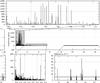 |
Fig. 1 Frequency diagram (units of d-1 on the x-axis, and ppm on the y-axis) containing all frequencies from the iterative prewhitening analysis. The centre panel shows the whole range of detected frequencies. The top panel is a zoom-in on the gravity mode region. The bottom right panel is a zoom-in on the pressure mode region (grey line is the detection threshold). The bottom left panel shows the intermediate region with two modes clearly standing out amongst the other frequencies. |
The long-term linear trend in the light curve is linked to the decline of the CCD’s gain (Auvergne et al. 2009). We treated it as a multiplicative instrumental effect and divided the light curve with a fitted linear polynomial. This way, we neglect a small deviation from the linear trend between day 70 and day 100, which is also visible in the light curves of the simultaneously observed A5 star HD 49862 and A2 star HD 49294, and is therefore probably of instrumental origin. This introduces low amplitude low frequencies (e.g. f013 in Table A.2). For a description of the noise properties and the window function, we refer to Degroote et al. (2009a), where a detailed analysis for LRc01 is presented.
We used an iterative prewhitening procedure, each time with a nonlinear update of the last 20 frequencies (see Degroote et al. 2010) to extract the frequency content from the CoRoT light curve. The results are shown in Fig. 1 and listed in Table A.2. This table contains a list of all frequency identification numbers, the amplitudes, frequency values and phases (including errors), as well as the signal-to-noise ratio (S/N) and the BIC value. All amplitudes range between 5 and 1800 ppm, or, equivalently, between 6 μmag and 1.8 mmag. The general trend is that at higher frequencies, the amplitudes become lower, with a few exceptions (e.g. f034 and f050). If we limit the analysis to the first 20 frequencies, no signs of nonlinear mode behaviour are detected in the frequency spectrum of HD 50230, neither in the form of harmonics nor higher-order combination frequencies (e.g. Fig. 2). If we include the frequencies beyond the first 20, we do identify harmonics and even combination frequencies. However, since the chance of finding combinations increases with the number of detected frequencies, these may be coincidental, and, therefore, only harmonics were taken into consideration. The frequencies for which harmonics have been detected are identified in Table A.2 in the last column, together with the relative strength present in the higher harmonics, compared to the main frequency. As an example, for f012, we list Ar(4) = 0.38, which means that four harmonics of f012 are detected, and that the sum of the amplitudes of all these harmonics amounts to 38% of the amplitude of f012 itself. Frequencies with a high Ar have a highly distorted phase shape (e.g. Fig. 3).
To test the validity of the sine model, the variance reduction was computed for an increasing number of single-sinusoids. Because our method of iteratively prewhitening sinusoids necessarily implies an increasing variance reduction, we computed the χ2 (with constant error terms) and Bayesian information criterion (BIC) as well (see also Degroote et al. 2009b). The latter criterion is only meaningful in a relative way, and weighs the introduction of extra parameters against the gain in variance reduction. The model with the lowest BIC value has the ideal number of parameters of all tested models. In general, the BIC and χ2 show a decreasing trend when more single-sinusoids are considered, which means that sinusoids are considered to be appropriate models to explain the observed variability (Fig. 4). When the BIC for each model is explicitly compared to the previous model, we conclude that in some cases adding three parameters to the model does not outweigh the resulting variance reduction. Because the BIC puts more weight on the number of parameters used, it puts the threshold for accepting sinusoids from the complete frequency analysis at ~200 frequencies (see Col. 9 in Table A.2), while the χ2 allows the use of 300 frequencies. Below these thresholds, the differences between the consecutive BIC and χ2 are no longer monotonically decreasing.
For the last nine frequencies of the 566 found from the linear frequency analysis, the BIC starts to rise, implying that the additional number of parameters are not worth the gain in variance reduction. This coincides with the use of a p-value of p = 0.1% as a stop criterion under the assumption of an exponential distribution of the Fourier periodogram, and a Bonferroni correction for multiple trial frequencies. The stepwise nonlinearly updated version of the frequency analysis finds nine frequencies less than the linear analysis (using the p value as stop criterion), while it still explains slightly more of the variance.
The high-amplitude gravity mode spectrum is discussed in detail by Degroote et al. (2010). For completeness, we list the frequencies connected to the period spacing in Table 1. They are also marked in italics in Table A.2. In the following, we focus on the (low-amplitude) features in the frequency spectrum above 1.5 d-1.
Periods and associated period spacings detected in the gravity mode spectrum.
2.2. Interpretation of the p-mode frequency spectrum
The majority of the frequencies above 1.5 d-1 have amplitudes below 50 ppm, making it difficult to separate them. The origin of these closely packed frequencies (between ~1.5 and ~5 d-1, see, e.g., the lower left panel in Fig. 1) is not obvious. They are not instrumental, since for quiet stars, the noise level of the CoRoT photometry is much lower. We do not expect them to be an artifact from the prewhitening procedure, partly because we used nonlinear optimisation, but mostly because the frequencies are located far away (≫1/T with T the total time span of the observations) from the dominant frequencies. They could originate from many closely spaced time-variable modes, or background stellar noise. A short-time Fourier transformation (STFT) shows hints for the time-variability of the modes (Fig. 5).
In addition, some time-independent frequencies clearly stand out, and are therefore good candidate pulsation modes (Fig. 1). This concerns 17 frequencies, marked in boldface in Table A.2. Some of these candidate pressure modes are isolated (Fig. 6), while others have a clear multiplet structure (Fig. 7, lower panel). In the STFT (Fig. 8), the latter show the typical interference patterns connected to beatings: when the spacing between two frequencies is x/T, we expect to see x times of constructive or destructive interference.
The autocorrelation of the periodogram between 10 and 15 d-1 (Fig. 7) reveals a well-resolved splitting Δfobs = 0.044 ± 0.007 d-1, possibly related to rotational splitting. For slow rotators, the rotational splitting of pressure modes can be approximated with (Ledoux 1951)
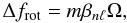 where βnℓ is dependent on the stellar structure, number of nodes n and degree ℓ, but typically close to unity. Ω is the rotation frequency of the star, and m the azimuthal order of the mode. The value of Δfobs is too low to be a large frequency separation between pressure modes of equal degree and consecutive radial order in the asymptotic approximation. Also, it is unlikely that this value is the low-frequency separation between modes of different degree, since the exact same pattern emerges around 10.4 d-1 and 11.6 d-1, which would imply that the large spacing is exactly the same for all degrees and that all modes of a given radial order but different degree cluster around the same value. The first-order interpretation of Δfobs as the rotation frequency Ω is compatible (but delivers no additional constraints) with stellar models between 5 and 10 M⊙ and stellar radii between 2 and 9 R⊙ and a projected rotational equatorial velocity veq ≈ 6.9 km s-1, with a restraint of the inclination angle i to be i > 20°.
A hint for a larger spacing around 0.8 d-1 is also discernible in the two panels of Fig. 7. The peak in the autocorrelation at 0.8 d-1 in the top panel of Fig. 7 is linked to the multiplets around 13.2 d-1 and 14 d-1 and the multiplets around 10.3 d-1 and 11 d-1. The peak at 1.25 d-1 is tied to the multiplets around 10.3 d-1 and 11.56 d-1. Detailed seismic modelling is needed to interpret this as a large frequency separation between equal-degree modes, though the radial order of these modes is probably too low to be in the asymptotic regime.
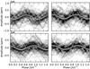 |
Fig. 2 Phase-folded light curves of the highest amplitude frequencies show that only one sine component is needed to fit the shape (from left to right, top to bottom: f001, f002, f004, and f005). The black dots are observations, the white circles are phase-binned averages, the thin grey line is a sine-fit (the exponent of the y-axis scale is given at the top of the plot). |
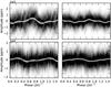 |
Fig. 3 Phase-folded light curves, using the frequencies (from left to right, top to bottom: f020, f033, f038, and f047). A clear deviation from the single-harmonic case in the form of a distorted phase shape is visible. For an explanation of the symbols, see Fig. 2. |
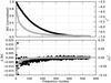 |
Fig. 4 Goodness-of-fit statistics of the sine-model. Both the BIC (black) and χ2 (grey) show a general decreasing trend (top panel), suggesting that sines are a good way of modelling the light curve. Despite the general decrease, however, not all frequencies are adequately modelled by sines: some frequencies in particular induce a worse BIC (ΔBIC > 0) (lower panel). |
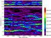 |
Fig. 5 Short-time Fourier transformation of the frequency region between 1.5 and 2.3 d-1 with a rectangular window of width 30 d-1. All signal outside of these regions is removed. Clear signal is present (colours denote squared amplitude in ppm2), and the frequencies and amplitudes show hints of variability. As a reference, the top panel shows a copy of the upper part of plot, where two artificial constant sine curves are introduced. |
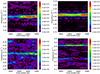 |
Fig. 6 Short-time Fourier transformations of four isolated frequencies in the high-frequency region (rectangular window of width 30 d-1, colours denote squared amplitude (ppm2)). In contrast to Fig. 5, the frequencies appear throughout the whole light curve. |
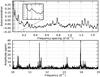 |
Fig. 7 Autocorrelation (upper panel) of the frequency spectrum (lower panel) between 10 and 15 d-1 (with the frequencies outside this region removed) uncovers a multiplet spacing of Δf = 0.044 d-1 that was measured between the peaks near ~10.4 d-1 and ~11.6 d-1. The peak around ~0.8 d-1 originates from the spacing between the structures around 13.2 d-1 and 14 d-1 (bottom panel), and those at 10.3 d-1 and 11 d-1. The thick grey line is plotted at a separation of 3/T for comparison with the frequency resolution. |
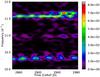 |
Fig. 8 The short-time Fourier transformation of the frequency region between 10 and 12 d-1 (with a Hamming window to improve the dynamical range, window width of 20 d-1). The typical succession of constructive and destructive interference are typical signs of a barely resolved multiplet structure. The separation between the frequencies is of the order of 6/T. |
3. Fundamental parameters
3.1. Multicolour photometry: an early B-type main sequence star
An estimate of the fundamental parameters of HD 50230 is obtained by fitting model atmospheres to observed multicolour photometry. We chose this approach over the application of existing calibration schemes (e.g., Cramer 1984), because fitting model atmospheres directly allows for an easy insertion of up-to-date atmosphere models, and allows for the combined use of different photometric systems. For early-type stars, the shape of the spectral energy distribution (SED) in the blue part, before (and including) the Balmer jump, is most sensitive to changes in the fundamental parameters. In general, SEDs are not very sensitive to binarity, because the luminosity scales with the square of the radius of the star and fourth power of effective temperature. For main sequence binaries, the brightest star is expected to be the hottest and the largest. To cover a wide spectral range and to emphasise the UV region, we collected TD1 (Thompson et al. 1978), ANS (Wesselius et al. 1982), Geneva (Mermilliod et al. 1997), and 2MASS (Cutri et al. 2003) measurements. Although there are also Johnson (Johnson 1965) measurements available, we decided not to include them here. The Johnson filter system is often used to denote a wide range of slightly different response curves, and including them does not increase the wavelength coverage.
To convert the Vega-system magnitudes to fluxes, we used the calibration of Rufener & Nicolet (1988), Maíz Apellániz (2006), and Wesselius et al. (1980) in combination with the Vega model of Bohlin & Gilliland (2004). We chose to fit the TLUSTY model atmospheres of Lanz & Hubeny (2007), because they include non-LTE effects, which can influence the shape of the SED of early-type stars.
The comparison between model atmospheres and observations for the determination of fundamental parameters was made via a grid-based approach as described in Degroote et al. (2011). The goodness-of-fit and confidence intervals (CI) of the parameters were determined using a χ2 statistic with five degrees of freedom (the effective temperature Teff, surface gravity log g, metallicity Z, interstellar reddening E(B − V), and angular diameter θ). Because of the grid-based approach, correlation effects on the parameter uncertainties are naturally taken into account.
Fundamental parameters of HD 50230 and their 95% CI.
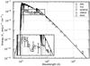 |
Fig. 9 Spectral energy distribution of HD 50230. Observations and their associated errors are shown with different open markers (see legend). Synthetic photometry from the best-fitting model (grey solid line, the unreddened model is shown as the black solid line) are marked with crosses. The inset is a zoom on the ultraviolet region. |
After fixing the fundamental parameters of HD 50230, we searched for near-infrared photometry obtained by the WISE satellite (Wright et al. 2010), which we calibrated following Cutri et al. (2011). We observed no significant infrared excess. The results are listed in Table 2 and the final SED is shown in Fig. 9.
3.2. Spectroscopy: a suspected binary
Between 11 October 2008 and 10 January 2012, we have gathered 60 high-resolution spectra from three different instruments: 17 spectra from the Coralie spectrograph (R ≈ 50 000, 3870−6900 Å, Baranne et al. 1996) mounted on the Euler telescope at La Silla (Chile), 40 spectra from the Hermes spectrograph (R ≈ 85 000, 3770–9000 Å, Raskin et al. 2011) on the Mercator telescope on La Palma (Spain), and four spectra from the Harps spectrograph in the high-efficiency mode (EGGS, R ≈ 80 000, 3800–6800 Å, Mayor et al. 2003) on the ESO 3.6 m telescope at La Silla (Chile). A full log of the observations can be found in Table A.1. The first column shows the UT of mid-exposure, the second column contains the name of the instrument, and the last two columns give the exposure time and S/N of the spectra around 4500 Å.
A first look at the spectra shows many narrow and shallow lines, suggesting a low projected rotational velocity. The high resolution of the Harps spectra allows the Fourier decomposition method (see, e.g., Simón-Díaz & Herrero 2007) to measure veqsini values as low as ~2 km s-1 irrespective of any additional pulsational broadening effects. To obtain the best possible value, we averaged the two highest signal-to-noise ratio spectra and applied the Fourier decomposition on a set of 78 lines (from ions AlII, AlIII, ArII, CII, FeII, FeIII, NII, NeI, OI, OII, SII, SIII, SiII, and SiIII), with depth and isolation as selection criteria. We derive veqsini = 6.9 ± 1.5 km s-1, assuming a linear limb-darkening law with ϵ = 0.35. This low value is consistent with the observation that the two peaks of the narrow MgII 4481 doublet are visibly separated. HD 50230 is therefore a slow rotator.
To improve the estimation of the fundamental parameters based on the spectral features, we constructed an average spectrum. The individual spectra were normalised via spline fits to the continuum, and were corrected for radial velocity shifts. The radial velocity of each spectrum was computed via the least-squares deconvolution algorithm (LSD) of Donati et al. (1997), with varying assumptions on the template spectra and selected lines. The measurements show a clear continuously rising trend during the three years of monitoring (Fig. 10). To check whether the variability is caused by pulsations or binarity, we used the generalised least-square method of Zechmeister & Kürster (2009) to fit sines and Keplerian orbits to the data. This method has the advantage over other period-finding algorithms such as the Scargle periodogram (Scargle 1982) that it also fits a constant term to the data, avoiding the problem of determining the average radial velocity in case of poor sampling. At the same time, the method still has the benefits of fitting functions directly to the data, in contrast to phase-binning methods such as the phase dispersion minimisation technique (Stellingwerf 1978). No significant periods are found. We conclude that the rising trend is most likely caused by a companion in a wide binary system. Instrumental zeropoint offsets, which can be of the order of 1.5 km s-1 (Uytterhoeven et al. 2008), are ruled out because the peak-to-peak difference is much larger and the trend is also visible in the spectra from Harps or Hermes only. This is confirmed in the time-average, radial-velocity-corrected spectrum, where broad absorption features are discernible. These are most apparent around the He and Si lines (Fig. 11), but also in the red wing of the Hα line, where a small asymmetry is observed (Fig. A.4, bottom right panel). It is highly unlikely that the broad features are due to pulsationally induced line profile variations, since they are not symmetric in the averaged spectra, and the deviation is only apparent close to the continuum.
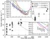 |
Fig. 10 Radial velocity derived from each individual spectrum via the LSD method. The inset in the upper left corner shows a zoom on an eight hour continuous monitoring of HD 50230, the inset in the lower right corner shows a zoom on a two-hour continuous monitoring. In colours, three fits with different frequencies are shown, vertically displaced to remove the day-to-day radial velocity shift. |
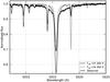 |
Fig. 11 HeI profile (black) of the averaged spectra. In grey, two single-star model HeI profiles are shown with different effective temperatures. No single adopted temperature can explain the wings of the profile, suggesting the presence of a broad-lined companion. |
3.3. Spectroscopic fundamental parameters
The fundamental parameters of HD 50230 as determined from photometry are listed in Table 2. The surface gravity is not constrained except for a lower limit of log g ≈ 3 dex. Alternatively, the fundamental parameters can be determined with the help of spectra in two ways: by fitting the line profiles directly with the help of synthesised spectra (e.g., Lehmann et al. 2011), or by comparing observed and predicted equivalent widths (EWs) (e.g., Morel et al. 2006). The former method has the advantage of a more concise way of handling blends, while the latter benefits from a reduction in the number of free parameters (i.e., veqsini and the radial velocity). We combined the two approaches by using the EW method (for a description of the grid, see Morel et al. 2006) to estimate the effective temperature of the primary component based on carefully selected lines, and turned to the spectral fitting method to incorporate the secondary component.
The EW-ratio of ions belonging to different ionisation stages of the same element are highly sensitive to changes in Teff, but are fairly insensitive to binarity, as long as the continuum flux ratio of both components is similar in the wavelength range under study, or trivially when the secondary component is not visible in the spectrum. In the temperature range between 16 000 and 22 000 K, useful ions are SiII and SiIII, and SII and SIII. For the Si lines, this includes the ratios of SiII6371 to SiIII4567, SiIII4574, SiIII5739 and SiIII4552. The SiII5041, SiII5056, SiII4128, and SiII4130 lines were discarded because of the uncertainties in the atomic modelling of these high-energy transitions (Simón-Díaz 2010). For the sulfur atom, we selected SII5032, SII4815, SII4230, SII4162, SII4716, SII4991, SII4294, SII4463, SII4824, SII4656, SII4792, SII4278, and SII4217 from the first ionisation stage, and SIII4284 and SIII4253 from the second ionisation stage. The observed EWs of the selected unblended features were calculated by numerical integration of the time-averaged normalised spectra (weighted with the S/N), and compared to the synthetic EWs. We find 17 500 < Teff < 19 500, and notice that lower surface gravity values imply lower effective temperatures (Fig. 12). We attempted to derive a value for the surface gravity and individual abundances by calculating the abundance of each element predicted by each individual line, adopting each log g parameter in the grid, and then minimising the scatter. These efforts failed, largely because of the unknown scaling factor that has to be included to compensate for the presence of the companion.
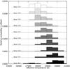 |
Fig. 12 Histograms of effective temperatures of the primary component derived from line ratios of SII/SIII and SiII/SiIII, assuming different values for the surface gravity log g. |
Subsequently, we use the χ2 fitting method to match the observed HARPS spectra with a grid of TLUSTY synthetic spectra (Lanz & Hubeny 2007) when Teff ≥ 15 000, and ATLAS synthetic spectra (Palacios et al. 2010) when Teff < 15 000. Because the secondary component is not visible in all selected lines, we first performed a grid search using a template spectrum of the HeI6678 line and varying the radial velocity of the component  and projected rotational velocity of the component
  . From this, we fixed the values to
  km s-1 and
  km s-1, though the uncertainties are several tens of km s-1 on both quantities. We assumed equal metallicities for both components, and demanded that the companion is less evolved than the primary (log g′ > log g). The χ2 minimisation method was performed with effective temperatures of the primary between 16 000 K and 22 000 K and between 15 000 K and 22 000 K for the secondary, surface gravities between 3.5 and 4.5 for the primary and secondary. The metallicity was chosen to be 0.1, 0.2, 0.5, or 1.0 times the solar value. For all 23 lines, the synthetic spectrum was calculated by taking the average of the synthetic profiles from the primary and secondary, weighted with the synthetic Eddington flux. Each ith profile was fitted to the data together with a linear continuum via
 and the total χ2 value was calculated as the squared sum of the residuals of all line profiles,
 where the index λ runs over all wavelengths in all profiles P. As an alternative test statistic, the χ2 was also calculated as the average of the
  values of all Np profiles,
 In the former statistic, the broad Balmer and helium profiles dominate because they cover a broader wavelength range. The latter statistic is designed to give equal weight to all profiles, regardless of the intrinsic width.
The fit procedure does not result in an accurate determination of the two components of the binary system, because the fits to several lines are not satisfactory (e.g., Figs. A.1–A.6). This could possibly be explained by shortcomings in atomic physics (e.g., in Si), or by metal mixtures significantly different from the solar mixture that is adopted in the models. A histogram weighted with the χ2-values sets the effective temperature and surface gravity of the primary at Teff = 17 000 K and log g = 3.5 (cgs), while the minimum χ2 is attained at Teff = 19 000 K and log g = 4.0 (cgs). This range is compatible with the temperature determination from the SED fit and the EW method, which are less influenced by the fainter companion. The effective temperature of the companion is Teff ≤ 15 000 K according to the χ2 fitting (the minimum is obtained at the edges of the grid), while the weighted histogram sets it to Teff = 16 000 K. The surface gravity is found to be between log g = 4.0 − 4.5 (cgs). The most likely value for the metallicity is half the solar value, but cannot be accurately determined from the used fitting procedure. A fit to all lines with Teff = 19 000 K and log g = 4.0 (cgs) for the primary, and Teff = 15 000 K and log g = 4.0 (cgs), is shown in Figs. A.1 to A.6. While the binary fit procedure fails at characterising the secondary, the binary line profile fits result in a better explanation for the asymmetry or broad line components in some of the lines. We conclude that Teff = 18 500 ± 1000 K and log g = 3.8 ± 0.3 (cgs) is an acceptable range for the fundamental parameters of the primary, and Teff ≤ 16 000 K and log g ~ 4 (cgs) for the secondary.
4. Line profile variability
Pulsational variability can cause radial velocity changes or variability in the line profile itself, depending on the degree and azimuthal order of the mode. They can be detected and identified via a pixel-to-pixel frequency analysis of the profiles (e.g., Zima 2006), or via characterisation of the line profile’s moments (Aerts et al. 1992). Given the narrow lines, we opted for the latter method.
The combination of the scarce time sampling of the spectroscopic measurements and the continuously rising trend in radial velocities (Fig. 10) impedes the detection of sinusoidal variability due to pulsations in the line profiles. For that reason, we applied a linear fit to both features simultaneously, using a function of the form ![Mathematical equation: \begin{equation} M(t_i) = a_0 + a_1 t_i + a_2\sin[2\pi(ft_i + a_3)].\label{eq:lin_plus_sine} \end{equation}](/articles/aa/full_html/2012/06/aa18548-11/aa18548-11-eq131.png) (1)Here, a0 and a1 represent the parameters of the straight-line fit, and a2, f, and a3 are the amplitude, frequency and phase of the sinusoidal component. We fitted the linear parameters aj to the time series of moments calculated at all observing times ti, for a grid of test frequencies f that includes all frequencies detected in the CoRoT light curve. To improve the SNR of the individual profiles, we used the LSD method (Donati et al. 1997) to compute the average profile of the deepest metallic spectral lines. From a fit evaluation via the F-statistic we conclude that there are no significant frequencies. A similar procedure excluding a linear trend also yields no significant frequencies.
(1)Here, a0 and a1 represent the parameters of the straight-line fit, and a2, f, and a3 are the amplitude, frequency and phase of the sinusoidal component. We fitted the linear parameters aj to the time series of moments calculated at all observing times ti, for a grid of test frequencies f that includes all frequencies detected in the CoRoT light curve. To improve the SNR of the individual profiles, we used the LSD method (Donati et al. 1997) to compute the average profile of the deepest metallic spectral lines. From a fit evaluation via the F-statistic we conclude that there are no significant frequencies. A similar procedure excluding a linear trend also yields no significant frequencies.
5. Discussion and conclusions
We classified HD 50230 as a wide double-lined spectroscopic binary consisting of a component with a low projected rotational velocity, and a component with a moderate projected rotation velocity. From the EW ratios, we established an effective temperature around 18 500 K for one component, which agrees with multicolour photometry. From this, we conclude that the narrow-lined component is the primary, and the broad-line component the (cooler) secondary. This is confirmed by a spectral line fitting procedure, where an upper limit for the effective temperature of 16 000 K is found. We estimate both stars to be main-sequence stars, and rule out the possibility of a subdwarf companion based on luminosity arguments, although their surface gravities could not be determined accurately from the wings of the Balmer lines, because of the blend of the two components.
The identification of HD 50230 as a spectroscopic binary complicates the interpretation of the light curve compared to the single-star hypothesis. However, the period spacing discovered in Degroote et al. (2010) is unlikely to be affected by the binary light curve, partially because of the high amplitudes of the modes considered, but mainly because the chance of observing such a regular pattern as the combination of two independent frequency patterns, are slim. Less obvious is the connection between the gravity modes and the pressure modes as originating from the same star. The companion is less luminous (the flux ratio is below 0.7) and cooler than the primary, placing it far below the β Cep instability strip. It is therefore unlikely to exhibit this family of pressure modes. Moreover, there are strong hints for rotationally split multiplets in the pressure mode regime, of which the narrow spacing is incompatible with fast rotation as occurs in the secondary component. Possibly, the low-frequency region is contaminated by the signal of the companion at low amplitudes because it resides in the SPB strip and may have a flux as high as half that of the primary. Even so, we do not expect that the gravity-mode spectrum, and in particular the gravity mode period spacing, originates from the companion, since cool B-type stars do not typically exhibit a variability spectrum this dense (see, e.g., Balona et al. 2011; Degroote et al. 2011). We finally remark that, although we give a list of 556 frequencies detected in the CoRoT light curve, the second half of that list should be taken with caution, because they do not satisfy the BIC criterion.
The spectroscopic line profiles show obvious signs of variability on short time scales. In particular, an eight-hour continuous monitoring of the star with HERMES shows a continuously declining trend in the radial velocities, in contrast to the previously described orbital rising trend. The data set at hand did not suffice, however, to find clear periodicities. The origin of this problem could lie in the dense gravity mode region, making the resulting complex beating pattern impossible to separate from the noise. It is hard to imagine, however, that we could detect frequencies in the line profile variations which are not present in the CoRoT light curve at photometric micromagnitude precision. This makes f034 ≈ 2.48 d-1 and f050 = 4.92 d-1 the most likely candidates for causing LPV. The latter frequency is excluded as the main contributor to the radial velocity dispersion, based on the eight-hour continuous observation run, which should cover at least one cycle. If we focus on the measurements taken in close succession phased to f034 (Fig. 10, red curve), we can see that this frequency is indeed likely to be present in the data, but other frequencies are equally successfull at fitting the observations (e.g., Fig. 10, blue and green curve).
In conclusion, we have gathered observational information to begin an in-depth seismic study of the hybrid B-type pulsator HD 50230. Despite its slow surface rotation of the order of veq ≈ 10 km s-1, the seismic modelling will have to take into account rotational effects when interpreting small deviations from uniform period spacings (Aerts & Dupret 2011). The ultimate future goal is to reconcile the observational information from the period spacings with that of the lower-order mode spectrum, which will allow a description of the whole interior of the star, from the convective core to the radiative envelope.
Online material
Appendix A: additional tables and figures
Logbook of spectroscopic observations.
Frequency list and statistics from a Fourier analysis with iterative nonlinear updates of the parameters.
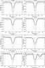 |
Fig. A.1 Binary fit to a selection of spectral lines. In grey, the average of all observed HARPS spectra of HD 50230 is plotted. Dashed black lines denote the contributions of the separate companions, the solid black line shows the obtained binary fit. Note that due to the simultaneous fitting of the continuum with the lines, the line continuum level can be off if the line does not fit well (i.e., the average quadratic distance between the observed and synthetic line profile is minimised). The fit consists of a primary component with Teff = 18 500 K and log g = 4.0 (cgs), and Teff = 15 000 K and log g = 4.0 (cgs) for the secondary. |
Acknowledgments
P.D. and C.A. are grateful for the hospitality during their stay at the Kavli Institute for Theoretical Physics in the framework of the Research Programme Asteroseismology in the Space Age. The research leading to these results has received funding from the European Research Council under the European Community’s Seventh Framework Programme (FP7/2007–2013)/ERC grant agreement No. 227224 (PROSPERITY), from the Belgian PRODEX Office under contract C90309: CoRoT Data Exploitation, and by the National Science Foundation of the United States under Grant No. NSF PHY05-51164.
References
- Aerts, C., & Dupret, M.-A. 2011 [arXiv:1108.6248] [Google Scholar]
- Aerts, C., de Pauw, M., & Waelkens, C. 1992, A&A, 266, 294 [NASA ADS] [Google Scholar]
- Auvergne, M., Bodin, P., Boisnard, L., et al. 2009, A&A, 506, 411 [NASA ADS] [CrossRef] [EDP Sciences] [Google Scholar]
- Baglin, A., Michel, E., Auvergne, M., & The COROT Team 2006, in Proc. of SOHO 18/GONG 2006/HELAS I, Beyond the spherical Sun, ESA SP, 624 [Google Scholar]
- Balona, L. A., Pigulski, A., Cat, P. D., et al. 2011, MNRAS, 298 [Google Scholar]
- Baranne, A., Queloz, D., Mayor, M., et al. 1996, A&AS, 119, 373 [NASA ADS] [CrossRef] [EDP Sciences] [Google Scholar]
- Bohlin, R. C., & Gilliland, R. L. 2004, AJ, 127, 3508 [NASA ADS] [CrossRef] [Google Scholar]
- Cramer, N. 1984, A&A, 141, 215 [NASA ADS] [Google Scholar]
- Cutri, R. M., Skrutskie, M. F., van Dyk, S., et al. 2003, 2MASS All Sky Catalog of point sources, NASA/IPAC Infrared Science Archive [Google Scholar]
- Cutri, R. M., Wright, E. L., Conrow, T., et al. 2011, Explanatory Supplement to the WISE Preliminary Data Release Products, Tech. Rep. [Google Scholar]
- De Ridder, J., Telting, J. H., Balona, L. A., et al. 2004, MNRAS, 351, 324 [NASA ADS] [CrossRef] [Google Scholar]
- Degroote, P., Aerts, C., Ollivier, M., et al. 2009a, A&A, 506, 471 [NASA ADS] [CrossRef] [EDP Sciences] [Google Scholar]
- Degroote, P., Briquet, M., Catala, C., et al. 2009b, A&A, 506, 111 [NASA ADS] [CrossRef] [EDP Sciences] [Google Scholar]
- Degroote, P., Aerts, C., Baglin, A., et al. 2010, Nature, 464, 259 [NASA ADS] [CrossRef] [PubMed] [Google Scholar]
- Degroote, P., Acke, B., Samadi, R., et al. 2011, A&A, 536, A82 [NASA ADS] [CrossRef] [EDP Sciences] [Google Scholar]
- Desmet, M., Briquet, M., Thoul, A., et al. 2009, MNRAS, 396, 1460 [NASA ADS] [CrossRef] [MathSciNet] [Google Scholar]
- Donati, J., Semel, M., Carter, B. D., Rees, D. E., & Collier Cameron, A. 1997, MNRAS, 291, 658 [NASA ADS] [CrossRef] [MathSciNet] [Google Scholar]
- Handler, G., Shobbrook, R. R., Jerzykiewicz, M., et al. 2004, MNRAS, 347, 454 [NASA ADS] [CrossRef] [Google Scholar]
- Handler, G., Jerzykiewicz, M., Rodríguez, E., et al. 2006, MNRAS, 365, 327 [NASA ADS] [CrossRef] [Google Scholar]
- Handler, G., Matthews, J. M., Eaton, J. A., et al. 2009, ApJ, 698, L56 [NASA ADS] [CrossRef] [Google Scholar]
- Johnson, H. L. 1965, ApJ, 141, 923 [NASA ADS] [CrossRef] [Google Scholar]
- Lanz, T., & Hubeny, I. 2007, ApJS, 169, 83 [CrossRef] [Google Scholar]
- Ledoux, P. 1951, ApJ, 114, 373 [NASA ADS] [CrossRef] [Google Scholar]
- Lehmann, H., Tkachenko, A., Semaan, T., et al. 2011, A&A, 526, A124 [NASA ADS] [CrossRef] [EDP Sciences] [Google Scholar]
- Maíz Apellániz, J. 2006, AJ, 131, 1184 [NASA ADS] [CrossRef] [Google Scholar]
- Mayor, M., Pepe, F., Queloz, D., et al. 2003, The Messenger, 114, 20 [NASA ADS] [Google Scholar]
- Mermilliod, J., Mermilliod, M., & Hauck, B. 1997, A&AS, 124, 349 [NASA ADS] [CrossRef] [EDP Sciences] [Google Scholar]
- Michel, E., Baglin, A., Auvergne, M., et al. 2006, in ESA SP 1306, ed. M. Fridlund, A. Baglin, J. Lochard, & L. Conroy, 39 [Google Scholar]
- Morel, T., Butler, K., Aerts, C., Neiner, C., & Briquet, M. 2006, A&A, 457, 651 [NASA ADS] [CrossRef] [EDP Sciences] [Google Scholar]
- Palacios, A., Gebran, M., Josselin, E., et al. 2010, A&A, 516, A13 [NASA ADS] [CrossRef] [EDP Sciences] [Google Scholar]
- Pojmanski, G. 2002, Acta Astron., 52, 397 [NASA ADS] [Google Scholar]
- Raskin, G., van Winckel, H., Hensberge, H., et al. 2011, A&A, 526, A69 [NASA ADS] [CrossRef] [EDP Sciences] [Google Scholar]
- Rufener, F., & Nicolet, B. 1988, A&A, 206, 357 [NASA ADS] [Google Scholar]
- Scargle, J. D. 1982, ApJ, 263, 835 [NASA ADS] [CrossRef] [Google Scholar]
- Simón-Díaz, S. 2010, A&A, 510, A22 [NASA ADS] [CrossRef] [EDP Sciences] [Google Scholar]
- Simón-Díaz, S., & Herrero, A. 2007, A&A, 468, 1063 [NASA ADS] [CrossRef] [EDP Sciences] [Google Scholar]
- Stellingwerf, R. F. 1978, ApJ, 224, 953 [NASA ADS] [CrossRef] [Google Scholar]
- Thompson, G. I., Nandy, K., Jamar, C., et al. 1978, Catalogue of stellar ultraviolet fluxes, A compilation of absolute stellar fluxes measured by the Sky Survey Telescope (S2/68) aboard the ESRO satellite TD-1 (NASA/STI) [Google Scholar]
- Uytterhoeven, K., Poretti, E., Rainer, M., et al. 2008, J. Phys. Conf. Ser., 118, 012077 [NASA ADS] [CrossRef] [Google Scholar]
- Wesselius, P. R., van Duinen, R. J., Aalders, J. W. G., & Kester, D. 1980, A&A, 85, 221 [NASA ADS] [Google Scholar]
- Wesselius, P. R., van Duinen, R. J., de Jonge, A. R. W., et al. 1982, A&AS, 49, 427 [NASA ADS] [Google Scholar]
- Wright, E. L., Eisenhardt, P. R. M., Mainzer, A. K., et al. 2010, AJ, 140, 1868 [NASA ADS] [CrossRef] [Google Scholar]
- Zechmeister, M., & Kürster, M. 2009, A&A, 496, 577 [NASA ADS] [CrossRef] [EDP Sciences] [Google Scholar]
- Zima, W. 2006, A&A, 455, 227 [NASA ADS] [CrossRef] [EDP Sciences] [Google Scholar]
All Tables
Frequency list and statistics from a Fourier analysis with iterative nonlinear updates of the parameters.
All Figures
|
Fig. 1 Frequency diagram (units of d-1 on the x-axis, and ppm on the y-axis) containing all frequencies from the iterative prewhitening analysis. The centre panel shows the whole range of detected frequencies. The top panel is a zoom-in on the gravity mode region. The bottom right panel is a zoom-in on the pressure mode region (grey line is the detection threshold). The bottom left panel shows the intermediate region with two modes clearly standing out amongst the other frequencies. |
| In the text | |
|
Fig. 2 Phase-folded light curves of the highest amplitude frequencies show that only one sine component is needed to fit the shape (from left to right, top to bottom: f001, f002, f004, and f005). The black dots are observations, the white circles are phase-binned averages, the thin grey line is a sine-fit (the exponent of the y-axis scale is given at the top of the plot). |
| In the text | |
|
Fig. 3 Phase-folded light curves, using the frequencies (from left to right, top to bottom: f020, f033, f038, and f047). A clear deviation from the single-harmonic case in the form of a distorted phase shape is visible. For an explanation of the symbols, see Fig. 2. |
| In the text | |
|
Fig. 4 Goodness-of-fit statistics of the sine-model. Both the BIC (black) and χ2 (grey) show a general decreasing trend (top panel), suggesting that sines are a good way of modelling the light curve. Despite the general decrease, however, not all frequencies are adequately modelled by sines: some frequencies in particular induce a worse BIC (ΔBIC > 0) (lower panel). |
| In the text | |
|
Fig. 5 Short-time Fourier transformation of the frequency region between 1.5 and 2.3 d-1 with a rectangular window of width 30 d-1. All signal outside of these regions is removed. Clear signal is present (colours denote squared amplitude in ppm2), and the frequencies and amplitudes show hints of variability. As a reference, the top panel shows a copy of the upper part of plot, where two artificial constant sine curves are introduced. |
| In the text | |
|
Fig. 6 Short-time Fourier transformations of four isolated frequencies in the high-frequency region (rectangular window of width 30 d-1, colours denote squared amplitude (ppm2)). In contrast to Fig. 5, the frequencies appear throughout the whole light curve. |
| In the text | |
|
Fig. 7 Autocorrelation (upper panel) of the frequency spectrum (lower panel) between 10 and 15 d-1 (with the frequencies outside this region removed) uncovers a multiplet spacing of Δf = 0.044 d-1 that was measured between the peaks near ~10.4 d-1 and ~11.6 d-1. The peak around ~0.8 d-1 originates from the spacing between the structures around 13.2 d-1 and 14 d-1 (bottom panel), and those at 10.3 d-1 and 11 d-1. The thick grey line is plotted at a separation of 3/T for comparison with the frequency resolution. |
| In the text | |
|
Fig. 8 The short-time Fourier transformation of the frequency region between 10 and 12 d-1 (with a Hamming window to improve the dynamical range, window width of 20 d-1). The typical succession of constructive and destructive interference are typical signs of a barely resolved multiplet structure. The separation between the frequencies is of the order of 6/T. |
| In the text | |
|
Fig. 9 Spectral energy distribution of HD 50230. Observations and their associated errors are shown with different open markers (see legend). Synthetic photometry from the best-fitting model (grey solid line, the unreddened model is shown as the black solid line) are marked with crosses. The inset is a zoom on the ultraviolet region. |
| In the text | |
|
Fig. 10 Radial velocity derived from each individual spectrum via the LSD method. The inset in the upper left corner shows a zoom on an eight hour continuous monitoring of HD 50230, the inset in the lower right corner shows a zoom on a two-hour continuous monitoring. In colours, three fits with different frequencies are shown, vertically displaced to remove the day-to-day radial velocity shift. |
| In the text | |
|
Fig. 11 HeI profile (black) of the averaged spectra. In grey, two single-star model HeI profiles are shown with different effective temperatures. No single adopted temperature can explain the wings of the profile, suggesting the presence of a broad-lined companion. |
| In the text | |
|
Fig. 12 Histograms of effective temperatures of the primary component derived from line ratios of SII/SIII and SiII/SiIII, assuming different values for the surface gravity log g. |
| In the text | |
|
Fig. A.1 Binary fit to a selection of spectral lines. In grey, the average of all observed HARPS spectra of HD 50230 is plotted. Dashed black lines denote the contributions of the separate companions, the solid black line shows the obtained binary fit. Note that due to the simultaneous fitting of the continuum with the lines, the line continuum level can be off if the line does not fit well (i.e., the average quadratic distance between the observed and synthetic line profile is minimised). The fit consists of a primary component with Teff = 18 500 K and log g = 4.0 (cgs), and Teff = 15 000 K and log g = 4.0 (cgs) for the secondary. |
| In the text | |
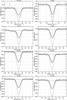 |
Fig. A.2 Same as Fig. A.1, but for additional spectral lines. |
| In the text | |
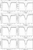 |
Fig. A.3 Same as Fig. A.1, but for additional spectral lines. |
| In the text | |
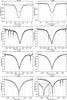 |
Fig. A.4 Same as Fig. A.1, but for additional spectral lines. |
| In the text | |
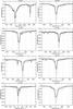 |
Fig. A.5 Same as Fig. A.1, but for additional spectral lines. |
| In the text | |
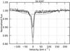 |
Fig. A.6 Same as Fig. A.1, but for additional spectral lines. |
| In the text | |
Current usage metrics show cumulative count of Article Views (full-text article views including HTML views, PDF and ePub downloads, according to the available data) and Abstracts Views on Vision4Press platform.
Data correspond to usage on the plateform after 2015. The current usage metrics is available 48-96 hours after online publication and is updated daily on week days.
Initial download of the metrics may take a while.