© ESO, 2012

1. Introduction

It is now understood that galactic winds may form an important evolutionary stage in galaxy evolution. In particular in the early universe, winds may be held responsible for polluting the intergalactic medium (IGM) with metals, possibly synthesized in Population III stars (e.g., Loewenstein 2001). The discovery of Lyman-Break galaxies (e.g., Steidel et al. 1996; Adelberger & Steidel 2000) has given much support to this idea. Evidence of winds at high redshift has been reported, e.g., by Dawson et al. (2002), who serendipitously discovered a strong asymmetric Ly_α emission line in a faint compact galaxy at z = 5.189, indicating an outflow velocity in the range of 320 − 360   km   s^-1.

In a recent study, it has been shown that many star-forming galaxies at 2 < z < 3 exhibit galactic outflows (Steidel et al. 2010). Apart from metal enrichment of the IGM, galactic winds are also thought to preheat the gas. The X-ray luminosity versus temperature relationship (L_X − T) shows a deviation from a power-law when going from massive to poor clusters of galaxies and groups. This has been interpreted in terms of a so-called “entropy floor” that dominates the gravitational heating of the cluster as the potential wells become shallower (Ponman et al. 1999). In other words, the preheating of the IGM by starburst driven galactic winds starts to dominate the release of gravitational energy. In addition, the fairly high metallicties of Z ~ 0.3   Z_⊙ (e.g., Molendi et al. 1999; Kikuchi et al. 1999) found in the intracluster gas may be explained by ejection of metals from galaxies by massive winds during starburst and also more quiescent phases (Kapferer et al. 2006).

In the local universe, evidence for galactic winds mainly stems from observations of starburst galaxies, such as M 82 or NGC 253. In these more evolved objects, starbursts are thought to be triggered by a substantial disturbance of the gravitational potential, e.g. by interaction with a companion galaxy. Finally, dwarf galaxies are prone to galactic winds because of their shallow gravitational potential well and their correspondingly low escape speeds, easily reached by supernova heated gas of a few 10⁶ K. According to Bernoulli’s equation, the typical outflow velocity, if all thermal is converted into kinetic energy, is on the order of v ≃ 250 km s^-1. In contrast, it is still widely believed that late-type spirals like the Milky Way should not exhibit winds, simply because the total thermal pressure in the disk is not sufficient to enable break-out through the extended gaseous HI layer and drive an outflow.

The situation though may be different in very active star forming regions, where superbubbles locally inject a substantial amount of energy enabling hot gas to reach considerable heights (Avillez & Breitschwerdt 2004, 2005). A related feature was observed in H_α by Reynolds et al. (2001) with WHAM. They find a giant loop extending out to  ~1300 pc perpendicular to the galactic plane. The base of the loop is spatially and kinematically connected to the HI chimney found by Normandeau et al. (1996), which is generated by the W4 star cluster. As more energy is deposited into this system by stellar winds and successive supernova explosions, we can expect the loop (the inner ionized part of the shell) to expand further and fragment due to Rayleigh-Taylor instabilities. The released hot plasma will then form the base of a galactic fountain, in which the gas may travel several kpc above the plane, but owing adiabatic and radiative cooling, thermal instabilities will progress and condensation of clouds (which are still gravitationally bound to the galaxy) is supposed to occur (Bregman 1980; Kahn 1981; Avillez 2000). Only if the combined thermal energy of breaking-out superbubbles exceeds the gravitational potential, a thermal galactic wind occur. In normal spirals this will only happen locally, and more extended winds are only expected in starburst regions like in M 82 or NGC 253.

However, as emphasized by many authors in the past (e.g., Axford 1981; Ipavich 1975; Breitschwerdt et al. 1991; Everett et al. 2008), the above argument ignores the effect of cosmic rays (CRs), which have an energy density that is roughly in equipartition with the thermal gas and the magnetic energy densities. The fact that CRs escape from the Galaxy after a few tens of million years on average, setting up a pressure gradient pointing away from the disk, gives rise to the resonant excitation of MHD waves via the so-called CR streaming instability (e.g., Kulsrud & Pearce 1969). Thus CRs are coupled to the thermal plasma by scattering off the frozen-in waves, thereby helping to push the plasma against the gravitational pull. As a result, CR transport, which is mainly diffusive in the disk, will predominantly become advective in the Galactic halo. Thus even in case of the Milky Way, a steady state wind flow could be set up with a global mass loss rate of  ~0.3   M_⊙   yr^-1 and a low outflow base velocity of  ~10 km s^-1 (Breitschwerdt et al. 1993). In fact, it has been shown that the diffuse broad-band soft X-ray background can be explained all the way from 0.3   keV to 1.5   keV by a superposition of emission from the Local Bubble and by a wind from the Galactic halo with both plasmas being in a state of nonequilibrium ionization (Breitschwerdt & Schmutzler 1994, 1999). Recently, Everett et al. (2008) have shown that a kiloparsec scale galactic wind of the Milky Way gives the best explanation for the longitude averaged soft X-ray emission near 0.65 and 0.85 keV observed with ROSAT PSPC. Their model is further constrained by simultaneously fitting the observed radio synchrotron emission, resulting in a higher pressure and smaller disk surface area wind (Everett et al. 2010).

Common to all investigations is the energy source due to more or less frequent supernova (SN) explosions, as well as to stellar winds, which contribute a minor fraction, and only during the initial phases, to the momentum and energy input, because only very massive O stars have sizable winds. For high stellar birth rates, therefore we can parameterize the results by the star formation rate (SFR) which relates the newly formed stars to the SN rate. In the case of low activity, the overall SN rate (types I and II) determines the properties of the globalgalactic wind. Assuming supernovae to be the sources of cosmic rays, we indeed expect CRs to accompany outflows from the disk into the halo, unless their coupling is very weak, and diffusion is the only mode of transport. However, as CR observations suggest, the diffusion halo only extends  ~ 1 − 3 kpc perpendicular to the disk (see Breitschwerdt et al. 2002). We therefore argue that CRs will always take part in the acceleration of an outflow, and although their effect may be small for starburst galaxies, it will dominate in the case of normal spirals.

On the other hand, advection of CRs in the galactic wind flow may lead to reacceleration of escaping disk particles in the energy range 3 × 10¹⁵ − 10¹⁷ eV (i.e. between the “knee” and the “ankle”) by propagating compressional waves as has been suggested by Völk & Zirakashvili (2004). These waves come from the interaction between fast outflows, originating in regions in the disk that have been compressed by the spiral density shock wave, hence have generated a faster CR driven outflow (cf. Breitschwerdt et al. 2002) and slower outflows from interarm regions. The steepening of the waves into moderate shocks of a sawtooth shape at large distances, where the flow is basically radial, leads to reaccelerating the particles close to the knee at a quasi-perpendicular shock (since the field is basically azimuthal there). Moreover, the supersonic galactic wind expands into the intergalactic medium with a given (but poorly known) pressure and must therefore be bounded by a termination shock, which itself can be the site of particle acceleration (Jokipii & Morfill 1985, 1987). It will, however, be difficult to observe these particles since they are advected away from the Galaxy with little chance to diffuse upstream to the disk. Since MHD turbulence downstream of the termination shock is presumably very strong, it acts in the model of Völk & Zirakashvili (2004) as a de facto reflecting boundary for the accelerated particles up to a certain energy. As the spiral density wave pattern is not in corotation with the disk and hence with the frozen-in halo field lines the associated forming halo shocks slip through the flux tubes.

In this paper we present an alternative possibility of accelerating particles in a galactic wind flow beyond the knee. The basic idea is that individual star-forming regions, e.g. superbubbles or localized starbursts, have an energy output that is not constant in time. Moreover, their lifetime is typically less than 10⁸ years and therefore smaller than the wind flow time. This will lead to time-dependent switch-off and switch-on effects of combined disk gas and CR outflows, which periodically push a piston into the gas. As we show in this paper, the galactic wind flow will be modulated by successive pairs of shocks (forward and reverse shock), where efficient particle acceleration can take place. Like the termination shock and unlike disk SNRs, these shocks will be long-lived, so the energy cut-off argument does not apply in this case because of finite size and acceleration time. They are thus strong candidates for generating the CR spectrum between 10¹⁵ eV and 10¹⁸ eV by post-acceleration of GCRs, as we shall see.

The paper is structured as follows. In Sect. 2 we describe the physical and numerical requirements of our model, and in Sect. 3 our general results from time-dependent galactic wind simulations for the Milky Way are presented, in particular the effect of particle diffusion and the propagation of shock waves within galactic winds. In Sect. 4 we introduce the interesting new possibility of accelerating cosmic rays by successive shock waves, which are driven by supernova explosions in the underlying disk, and propagate into the halo. A discussion and our conclusions are given in Sect. 5.

2. Galactic wind model

2.1. Physical equations

When employing the usual physical notation, we use the following time-dependent system of hydrodynamical equations supplemented by three energy density equations for the thermal gas, E_g, the cosmic rays, E_c, and the Alfvénic waves E_w: $\begin{array}{ccc}& & \frac{\mathit{\partial \rho }}{\mathit{\partial t}}\mathrm{+}\mathrm{\nabla }\mathrm{·}\mathrm{\left(}\mathit{\rho }{u}\mathrm{\right)}\mathrm{=}\mathrm{0}\\ & & \frac{\mathit{\partial \rho }{u}}{\mathit{\partial t}}\mathrm{+}\mathrm{\nabla }\mathrm{·}\mathrm{\left(}\mathit{\rho }{u}\mathrm{:}{u}\mathrm{\right)}\mathrm{+}\mathrm{\nabla }\mathrm{(}{\mathit{P}}_{\mathrm{g}}\mathrm{+}{\mathit{P}}_{\mathrm{c}}\mathrm{+}{\mathit{P}}_{\mathrm{w}}\mathrm{)}\mathrm{+}\mathit{\rho }\mathrm{\nabla }{\mathrm{\Phi }}_{\mathrm{gal}}\mathrm{=}\mathrm{0}\\ & & \frac{\mathit{\partial }{\mathit{E}}_{\mathrm{g}}}{\mathit{\partial t}}\mathrm{+}\mathrm{\nabla }\mathrm{·}\mathrm{\left(}{\mathit{E}}_{\mathrm{g}}{u}\mathrm{\right)}\mathrm{+}{\mathit{P}}_{\mathrm{g}}\mathrm{\nabla }\mathrm{·}{u}\mathrm{=}\mathrm{\Gamma }\mathrm{-}\mathrm{\Lambda }\\ & & \frac{\mathit{\partial }{\mathit{E}}_{\mathrm{c}}}{\mathit{\partial t}}\mathrm{+}\mathrm{\nabla }\mathrm{·}\left(\mathrm{\left(}{\mathit{E}}_{\mathrm{c}}\mathrm{\right(}{u}\mathrm{+}{\mathit{\gamma }}_{\mathrm{c}}{v}\mathrm{A}\mathrm{)}\right)\mathrm{+}{\mathit{P}}_{\mathrm{c}}\mathrm{\nabla }\mathrm{·}{u}\mathrm{-}{v}\mathrm{A}\mathrm{\nabla }{\mathit{P}}_{\mathrm{c}}\mathrm{=}\mathrm{\nabla }\mathrm{·}\mathrm{\left(}\mathit{\kappa ̅}\mathrm{\nabla }{\mathit{E}}_{\mathrm{c}}\mathrm{\right)}\\ & & \frac{\mathit{\partial }{\mathit{E}}_{\mathrm{w}}}{\mathit{\partial t}}\mathrm{+}\mathrm{\nabla }\mathrm{·}\left({\mathit{E}}_{\mathrm{w}}\mathrm{(}{u}\mathrm{+}{v}\mathrm{A}\mathrm{)}\right)\mathrm{+}{\mathit{P}}_{\mathrm{w}}\mathrm{\nabla }\mathrm{·}{u}\mathrm{+}{v}\mathrm{A}\mathrm{\nabla }{\mathit{P}}_{\mathrm{c}}\mathrm{=}\mathrm{0.}\end{array}$The Alfvén velocity is denoted by v_A, the bulk gas velocity by u, its density and pressure by ρ and P_g, respectively, while the CR and MHD wave pressures are labeled by P_c and P_w. The galactic gravitational potential is Φ_gal, which we take from Breitschwerdt et al. (1991), who used a Miyamoto-Nagai potential for the disk and bulge, as well as a spherical dark matter component. Additional heating Γ and cooling Λ can be included and an energy sink for cosmic rays is incorporated by v_A∇P_c, transferring energy from the cosmic rays to the waves due to the streaming instability. Energy sinks for the MHD waves other than adiabatic losses, e.g. ion-neutral or nonlinear Landau damping are not included (for a detailed discussion see Ptuskin 1997). The former is neglected because the level of ionization can be easily maintained in a tenuous hot outflow plasma, and the latter is expected to definitely become important, once the fluctuation amplitude reaches δB/B ~ 1, when quasilinear theory breaks down. Since we start with a negligible wave field, assuming that all outgoing waves are generated by the resonant instability, damping conditions in most model runs occur only farther out in the flow, where for example particle acceleration has already taken place. However, in general the effect of nonlinear Landau damping should not be neglected (see also discussion in Everett et al. 2008). Finally, in the case of thermally driven winds, such as in starburst galaxies, the contribution to the thermal pressure by wave damping is generally small, because the fraction of CR energy density is lower than the thermal one.

The above system is closed by the equation of states relating the pressures to the energies by ${\mathit{P}}_{\mathrm{c}\mathit{,}\mathrm{g}\mathit{,}\mathrm{w}}\mathrm{=}\mathrm{(}{\mathit{\gamma }}_{\mathrm{c}\mathit{,}\mathrm{g}\mathit{,}\mathrm{w}}\mathrm{-}\mathrm{1}\mathrm{)}\hspace{0.17em}{\mathit{E}}_{\mathrm{c}\mathit{,}\mathrm{g}\mathit{,}\mathrm{w}}\mathit{.}$(6)Assuming ultrarelativistic particles, we adopt γ_c = 4/3, and taking a monoatomic gas, we set γ_g = 5/3. A value of γ_w = 3/2 corresponds to a wave energy density E_w =  ⟨ (δB)² ⟩ /4π of the mean squared fluctuating magnetic field component. Since the magnetic wave pressure is given by P_w =  ⟨ (δB)² ⟩ /8π, we obtaina value of γ_w = 3/2 by analogy. We also have to specify the mean diffusion coefficient for the cosmic rays (Drury 1983), which is averaged over the particle distribution function (in space and momentum), and is usually taken to be a free parameter. According to cosmic ray propagation models (e.g., Ginzburg & Ptuskin 1985), is estimated as an order of 10²⁹   cm²   s^-1.

In the self-consistent CR propagation model of Ptuskin et al. (1997), the field parallel diffusion coefficient is calculated from the MHD turbulence level arising from CR streaming, with generation balanced by nonlinear Landau damping, so that $\mathit{\kappa ̅}{}_{\mathrm{\parallel }}\mathrm{\simeq }{\mathrm{10}}^{\mathrm{27}}{{}^{\mathrm{\right(}}\frac{\mathit{p}}{\mathit{Zmc}}^{\mathrm{\left)}}}^{\mathit{q}\mathrm{-}\mathrm{3}} \mathrm{c}{\mathrm{m}}^{\mathrm{2}}\hspace{0.17em}{\mathrm{s}}^{-1}$, for Galactic halo conditions, where q ≈ 4 is the power-law index in the particle momentum distribution near CR sources, and p,m, and Z are the particle momentum, mass and nuclear charge, respectively. The influence of particle diffusion and acceleration is discussed in Sect. 3.1 and more detailed properties of the system of Eqs. (1)–(6) can be found in Breitschwerdt et al. (1991).

These equations are solved in a 1D flux tube geometry, where all quantities depend on the projected distance z from the galactic plane and the time t. To fix ideas we specify the geometric properties of the flux tube, which represents a transition from planar to spherical flow, and is in its simplest form written as $\mathit{A}\mathrm{\left(}\mathit{z}\mathrm{\right)}\mathrm{=}{\mathit{A}}_{\mathrm{0}}\left[\mathrm{1}\mathrm{+}{\left(\frac{\mathit{z}}{{\mathit{z}}_{\mathrm{0}}}\right)}^{\mathrm{2}}\right]\mathit{,}$(7)where z₀ defines a typical scale above which the flux tube opens due to spherical divergence (typically of the order of a galactic radius). For short distances z ≪ z₀, the flow is essentially planar and as seen e.g. in Table 1 the lower values of z₀ lead to faster shocks propagating along the flux tube. A₀ denotes the cross section at our reference level of z = 0, which cancels out in all equations.

It has been emphasized by some authors that the equations should be written and solved in general ellipsoidal (Fichtner et al. 1991) or at least in oblate spheroidal coordinates (Ko 1991). A test of the simple formulation of Eq. (7) in comparison to oblate spheroidal coordinates has shown that the maximum deviation is an enhancement of the mass loss rate by about 15% for a flux tube at a Galactocentric distance of R₀ = 10 kpc (Breitschwerdt 1994). The discrepancy even decreases for shorter distances, because the effect of a radial (as opposed to vertical) flow component becomes progressively weaker. In addition, it is more likely that the injection of supernova heated gas into the base of the halo also imparts a z-component of momentum to the flow, again enhancing the vertical component. Thus, for practical purposes, Eq. (7) seems fairly robust and time saving, and only a complete solution of the axisymmetric MHD equations, in which the surfaces of magnetic pressure are calculated self-consistently by a Grad-Shafranov type equation, marks a substantial improvement. Here we are primarily concerned with the interplay of various physical processes and the rôle of cosmic rays as a driving agent, and so we take advantage of the simple but flexible flux tube formulation in Eq. (7).

As seen e.g. in Eq. (15), the assumed flux tube geometry also determines the radial structure of the magnetic field. However, edge-on observations of spiral galaxies like NGC 5775 reveal large scale magnetic fields of similar topology in their galactic halo (Soida et al. 2011). Also recent 3D-numerical simulations of a cosmic ray driven dynamo (Kulpa-Dybel et al. 2011) show that random magnetic fields will evolve into large-scale, ordered magnetic structures that reveal a quadrupole-like configuration with respect to the galactic plane. Observationally, as well as theoretically, assuming a prescribed flux-tube geometry thus seems appropriate for simplifying the time-dependent evolution of galactic winds through this 1D-geometry.

To summarize the previous section we have shown how to set up a system of equations that describes a galactic outflow driven by the interplay of the gravitational potential and the interaction of thermal gas, cosmic rays, and waves in an ad-hoc prescribed geometry. Several outflow simulations are discussed in detail in the following sections. The time-dependent effects of dissipation, heating and cooling, as well as particle acceleration lead to a number of features, which in most cases can be followed until a time-independent, stationary solution is reached.

2.2. Boundary conditions

Boundary conditions close to the disk have to be specified, allowing for a transition from a subsonic to a supersonic outflow. In steady state this is only possible if the outward pressure tends to zero at infinity, as shown by Parker (1958) for the solar wind. The terminal wind velocity can be easily estimated from Bernoulli’s equation. At the inner boundary located at a reference level, we have to fix, e.g., the gas density, the gas, and wave pressure. The cosmic rays are determined by an outward directed flux ${F}\mathrm{c}\mathit{,}\mathrm{0}\mathrm{=}\frac{{\mathit{\gamma }}_{\mathrm{c}}}{{\mathit{\gamma }}_{\mathrm{c}}\mathrm{-}\mathrm{1}}\mathrm{(}{u}\mathrm{0}\mathrm{+}{{v}\mathrm{A}}_{\mathrm{0}}\mathrm{)}{\mathit{P}}_{\mathrm{c}\mathit{,}\mathrm{0}}\mathrm{-}{\frac{\mathit{\kappa ̅}}{{\mathit{\gamma }}_{\mathrm{c}}\mathrm{-}\mathrm{1}}\frac{\mathit{\partial }{\mathit{P}}_{\mathrm{c}}}{\mathit{\partial z}}|}_{\mathrm{0}}\mathit{,}$(8)where the first part describes the advected particles through the combined wave speed u₀ + v_A0, and the second term represents the diffusive flux across the inner boundary. Since energetic particles always leave the galaxy within a so-called residence time (about  ~ 10⁷ yr for the Milky Way), we have to ensure F_c,0 > 0. If we use a typical length scale L to approximate the diffusive term in Eq. (8) by P_c,0/L, we can calculate on which scale the cosmic ray flux would vanish, i.e., F_c,0 = 0 or . Even in the case of low , we obtain L > 1   Mpc, hence F_c,0 > 0 for all realistic galactic parameters since the Alfvén velocity is |v_A0| = 6.9   km   s^-1 for our initial conditions. The last quantity to be specified at the inner boundary is the velocity u₀, which in case of a steady-state solution is determined by the conditions at the critical point, thereby fixing the mass loss rate.

At the outer boundary we impose simple outflow conditions; i.e., no gradients should exist at large distances from the galactic plane, typically at z = 1000   kpc. As studied in various computations the details of the outer boundary do not change the overall behavior of the solutions. In steady-state flows, the domain of influence of the inner boundary conditions only encloses the subsonic flow region. The location of the critical point, however, is not completely independent of the outer boundary conditions. In particular, it is required that the pressure at the sonic point exceeds the pressure at the outer boundary. Otherwise, no transsonic flows are possible and only breeze solutions will exist. For time-dependent flows such restrictions do not apply in general, and only in the time-asymptotic limit do comparisons with steady-state flows make sense.

As described in the following sections, we have computed time-dependent galactic winds arising from changes of the inner boundary conditions. In particular, we studied how these variations can be traced in the outflow and how the perturbed solution evolves towards a stationary flow.

2.3. Numerical method

Since the numerical method has been described in detail (Dorfi 1998), we emphasize here only some important features. First, all equations are cast into a volume-integrated form to ensure conservation of global quantities such as mass, momentum, and energy. Such a finite volume formulation is also suited to an adaptive grid that concentrates grid points to resolve steep gradients. Second, the equations are discretized in an implicit way so that for stationary solutions the time step exceeds the typical flow time by several orders of magnitude. Third, an artificial viscosity with a variable length scale in the tensor formulation (Tscharnuter & Winkler 1979) is adopted to broaden the shock waves over a finite number of grid points. However, since we also use an adaptive grid, the typical broadening length scale l_visc can be specified to be smaller than all physical length scales, which enables correct computation of particle acceleration; i.e., with u_s denoting the shock speed. The first-order Fermi mechanism requires that the energetic particles are exposed to a sharp discontinuity to gain energy by being reflected between the upstream and downstream media.

Applying the adaptive grid to these computations has the advantage that the position of discontinuities can be located very precisely through a clustering of grid points without specifying the type of nonlinear wave beforehand. The propagation of such nonlinear waves is plotted, e.g., in Fig. 4, which enables a direct comparison with analytic estimates.

Computations based on an implicit method have the advantage of allowing calculations of stationary solutions with the same numerical method as for the time-dependent solutions. As a result several solutions with fixed inner boundary values develop towards the stationary solutions, all of which can be reached from different evolutionary paths. We found from such a large number of calculations that the stationary solutions look rather stable with respect to perturbations and that time-dependent flows relax to the steady-state after the initial perturbations have propagated through the computational domain. For our Milky Way with a typical flow speed around 500   km   s^-1 we get a typical relaxation time of about 10⁹   years for a spatial region of 1   Mpc. The initial models can be taken directly from the time-independent solutions of Breitschwerdt et al. (1991).

The actual discrete equations are then solved by a nonlinear Newton-Raphson procedure and are given in the appendices. The total number of spatial grid points is set to 300 throughout the computations. Due to our six physical variables (gas density, gas velocity, thermal pressure, cosmic ray pressure, wave pressure and radial position) at every grid point, each time step requires 1800 new unknowns to be computed.

3. Results

3.1. Effects of cosmic ray diffusion

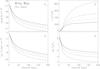Fig. 1 The time-asymptotic flow structure of a galactic wind up to the innermost 200   kpc with different cosmic ray diffusion coefficients . The case (full line) is almost identical to , and noticeable differences occur only for (dotted line), (dashed line), and (dashed-dotted line). The different panels represent: a) gas density; b) gas velocity; c) thermal gas pressure, d) ratio of gas pressure to cosmic ray pressure.

Before we compute time-dependent solutions of the system of CR-hydrodynamics in a flux tube geometry (Eqs. (1)–(5)) we investigate the effects of cosmic ray diffusion in steady state solutions. The additional diffusive term written as $\mathrm{\nabla }\mathrm{·}\mathrm{\left(}\mathit{\kappa ̅}\mathrm{\nabla }{\mathit{P}}_{\mathrm{c}}\mathrm{\right)}$(9)increases the order of the system of equations and no simple and straightforward analysis of critical points can be used to characterize the solutions. As emphasized earlier the implicit character of our numerical methods makes it easy to implement such an additional transport mechanism and in Fig. 1 the influence of a mean diffusion coefficient is shown.

The spatial wind profiles plotted in Fig. 1 exhibit the changes of the overall flow structure caused by different cosmic ray diffusion coefficients in the astrophysical relevant parameter range of within the innermost 200   kpc. Starting at a reference level of 1   kpc, we follow the flow up to a distance of 1000   kpc in order to reach asymptotic values. For these computations the numerical parameters correspond to our Galaxy, and we keep fixed most quantities at the inner boundary, i.e. the gas density of ρ₀ = 1.67 × 10^-27   g   cm^-3, the thermal gas pressure P_g,0 = 2.8 × 10^-13   dyne   cm^-2, the vertical magnetic field component B₀ = 1   μG, and the initial wave pressure P_w,0 = 4 × 10^-16   dyne   cm^-2, which corresponds to magnetic fluctuations at a low level of 0.1   B₀. In the case of no diffusion (), the mass flux and therefore the initial velocity u₀ are determined by the critical point (CP) conditions and left as a free inflow boundary for the diffusive cases. To investigate the effect of cosmic ray diffusion we fixed the total cosmic ray flux F_c,0 at the inner boundary through condition (8).

Since the diffusion length scale L associated with a flow velocity U and diffusion coefficient is determined through , i.e., for a typical value of U ≃ 300   km   s^-1 and of , we get L ≃ 1   kpc, so significant modifications of the large scale behavior are only expected for values of the mean diffusion coefficient , as can be seen in Fig. 1 for the Milky Way. Since the energetic particles can make an important contribution to the overall galactic gas outflow, the coupling of CRs to the gas is an important process that alters the mass loss rate of the wind. In the case of diffusive losses, CRs can escape from a galaxy without having to drag thermal gas along. To compare the solutions, the total cosmic ray flux F_c,0 is kept constant in Fig. 1 and therefore an increase in the diffusive losses has to be compensated by a corresponding decrease in the advection of particles at the reference level; i.e., u₀ decreases. Since the mass flux (per unit area) is given by ρ₀u₀, diffusion reduces the amount of thermal material within a flux tube. Consequently, any increase in the diffusion coefficient leads to lighter and faster winds with lower mass loss rates. Since the parameters for this computation are chosen for our own galaxy similar to Breitschwerdt et al. (1991), cosmic rays provide the dominant pressure contribution above 10   kpc for all values of as can be inferred from Fig. 1d. This is because even for the highest value of the diffusion length does not exceed 10   kpc. We emphasize that the solutions shown in Fig. 1 for for gas density, outflow velocity, thermal, CR, and wave pressures, all as a function of distance, are in excellent agreement with the steady-state solutions obtained in Breitschwerdt et al. (1991).

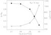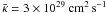
Fig. 2 Relative mass-loss rates (filled symbols) Ṁ in units of Ṁ0, the mass-loss rate at , and corresponding terminal velocities (open symbols) in  [km   s-1]  for a flux tube located in our Galaxy at a galactocentric distance of R0 = 10   kpc as a function of the mean cosmic ray diffusion coefficient . Only values of reduce the mass loss rate significantly, but also increase the final wind velocities owing to lower thermal gas ejections (see text for details).

The cosmic rays affect the inner boundary through the ingoing cosmic ray flux F_c,0 (Eq. (8)) as well as the transport of material through the flux tube thanks to the available cosmic ray pressure gradient. The increase in the mean cosmic ray diffusion coefficient leads to changes in the mass-loss rate and the final velocity as is shown in Fig. 2. Since in the adopted flux tube geometry for stationary winds the mass-loss rate is given by 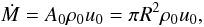$\mathit{Ṁ}\mathrm{=}{\mathit{A}}_{\mathrm{0}}{\mathit{\rho }}_{\mathrm{0}}{\mathit{u}}_{\mathrm{0}}\mathrm{=}\mathit{\pi }{\mathit{R}}^{\mathrm{2}}{\mathit{\rho }}_{\mathrm{0}}{\mathit{u}}_{\mathrm{0}}\mathit{,}$(10)we have plotted in Fig. 2 the mass loss relative to the case without cosmic ray diffusion, i.e. , and denote this value by Ṁ₀. Therefore we get rid of the scaling by the initial cross section of the flux tube A₀ = πR². This figure shows how the total mass loss is decreasing as the relative contribution of cosmic ray diffusion increases compared to the advected flux  ∝ (u₀ + v_A)P_c,0 for a fixed value of the total CR-flux F_c,0 at the inner boundary (cf. Eq. (8)). As stated before, the typical length scale of cosmic ray interactions on a flow with velocity U is given by , which alters the cosmic ray pressure gradients available to drive the outflow. As seen in Fig. 2 values of only have a small effect on the outflow characteristics, because such values are associated with length scales around 1   kpc taking a typical flow velocity of U ~ 300   km   s^-1. Comparing the results for various simulations of galactic winds from our Galaxy (Fig. 1), we conclude that only mean cosmic ray diffusion coefficients above affects the final outflow velocities and mass loss rates significantly. Constraints based on galactic cosmic ray observations indicate a diffusion coefficient on the order of  ~10²⁹   cm²   s^-1, for nucleons below about a GeV (e.g., Axford 1981), which represent the bulk of the particles, and somewhat higher values  ~10³⁰   cm²   s^-1 for particles with higher energies. In addition, the generation and propagation direction of Alfvén waves are influenced by the cosmic ray gradients (e.g., Breitschwerdt et al. 1991). However, if parameters that are appropriate for different galaxies only make a minor contribution to the wave pressure compared to the gas and cosmic ray pressures, this effect is almost negligible here (see also Figs. 3d and 5d).

All results reported here were calculated for a Miyamoto-Nagai galactic potential as used for our Milky Way at a galactocentric distance of R₀ = 10   kpc. This is slightly higher than the IAU value for the solar circle, but has been adopted here in order to compare results with Breitschwerdt et al. (1991). The dependence on the location within a galaxy enters only directly through a variation in the galactic potential Φ_gal, and indirectly by changes in gas density, pressure etc., as discussed in Breitschwerdt et al. (1991). Integrating their galactic winds solutions over the whole galactic disc yields a total mass loss rate of Ṁ_gal ~ 0.3   M_⊙   yr^-1. This can serve as an upper limit of the global galactic mass loss rate since the effect of cosmic ray diffusion (Fig. 2) will reduce this value, which was calculated from purely advective solutions.

Since the outflow velocity in case of thermally driven winds is usually more than an order of magnitude above the escape velocity, the mode of CR transport is immaterial here, since the mass loss rate itself is mainly determined by the thermal pressure. This is a consequence of the softer equation of state of the CRs, as compared to the thermal plasma, which leads to an efficient lifting of the halo weight at larger heights, when the mass density is already smaller. In terms of galactic wind flows, the thermal plasma gradient lifts up the gas close to the disk, and the CRs act as a kind of afterburner, accelerating the sluggish thermal winds to higher velocities. This effect is obviously exacerbated by an increasing CR diffusion coefficient.

The flow time through the wind is given in our computational domain by 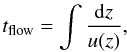${\mathit{t}}_{\mathrm{flow}}\mathrm{=}\mathrm{\int }\frac{\mathrm{d}\mathit{z}}{\mathit{u}\mathrm{\left(}\mathit{z}\mathrm{\right)}}\mathit{,}$(11)where the boundaries have to be taken e.g. between 1   kpc and 1   Mpc. In accordance with higher outflow velocities for increasing cosmic ray diffusive transport the flow times up to 1   Mpc decrease from 4.1 × 10⁹   years () to 2.8 × 10⁹   years in the case of . The flow times or final velocities do not scale directly with the mass loss rates (Fig. 2) since increasing the diffusion changes the inner boundary conditions (Eq. (8)) and also lowers the cosmic ray gradients needed to further accelerate the outflow. The sonic point of the galactic winds shrinks from 108   kpc to 48   kpc.

3.2. Time-dependent flow features

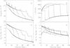Fig. 3 The time-dependent flow structure of a galactic wind up to 100   kpc at six different times at 3.4 × 106, 2.0 × 107, 3.6 × 107, 5.4 × 107, 7.7 × 107 and 1.0 × 108   years. At t = 0 the gas and cosmic ray pressure has been increased by a factor of 10 at the inner boundary of the flux tube, simulating a violent SN-explosion. Panel a) plots the development of the density structure where the forward as well as the reverse shock become visible. The velocity in  [km   s-1]  is depicted in panel b) where the particle acceleration broadens the shock fronts in time. In panels c) and d) the curves correspond to the gas and the cosmic ray pressure (solid line) together with the wave pressure (dashed lines), respectively. The velocities of these features are also plotted in Figs. 4 and 6 (see text for more details).

Assuming that the flux tube geometry is given and fixed in time we expect at least time-dependent inner boundary conditions. In a realistic case of repeated SN-explosions or a starburst event (on larger scales), the inner variations will be determined by the temporal history of such explosive events. Every change at the base of the flow introduces additional disturbances, which then propagate outwards and modify the flow conditions along the flux tube. To keep these structural changes simple and to illustrate the time-dependent behavior of a galactic wind, we have chosen a stationary model as our initial model with a flux tube opening distance z₀ = 15   kpc and a mean cosmic ray diffusion coefficient of , plotted also as dotted line in Fig. 1. The propagation of waves is driven by a sudden increase in gas and cosmic ray pressure at the inner boundary located at 1   kpc, where we have raised the pressures by a factor of 10 over a time interval of 10⁶   years. All other parameters are kept constant. Since we use an implicit numerical method, we can follow the propagation of these pressure waves through the whole computational domain until a new stationary solution has been established within 1 ≤ z/ [kpc]  ≤ 1000. Typically, the flow time (Eq. (11)) up to 1   Mpc is of a few 10⁹   years.

As plotted in Fig. 3 for the innermost 100   kpc the changes at the inner boundary result in a propagation of strong nonlinear waves along the flux tube since the conditions at the base of a galactic wind have been altered dramatically. In the simulations reported here, we keep the situation as simple as possible and see how pressure waves are initiated and generate a flow pattern similar to a supernova remnant (SNR) (e.g., Dorfi 1991). A strong forward shock wave propagates through the unperturbed wind structure, accompanied by a reverse or terminal shock, which slows down the newly developed outflow. However, owing to the high density and pressure gradients within the initial flux tube, the overall properties of the shock waves cannot be characterized by a rather simple self-similar behavior, which is typical of the SNR case. At both shock waves, particles are accelerated, which modifies the shock structure itself, and the dissipation of waves heats the thermal gas. The maximum momentum p_max of the accelerated particles attainable in such a shock configuration is plotted in Fig. 7, resulting in a reacceleration of the Galactic cosmic rays already driving the outflow. At the moment we have not included any radiative losses of the thermal plasma in our computations. Radiative cooling should not be dramatic close to the disk where the temperature is still above 10⁶ K and where the bulk of the particles are post-accelerated. At greater distances, when the temperature and density have dropped, cooling times (which are proportional to 1/ρ) still remain high.

In Fig. 3a the gas density clearly exhibits the separation of the flow structures between 3.6 × 10⁷   years and 1.0 × 10⁸   years since the forward shock propagates finally at a speed of 930   km   s^-1, whereas the reverse shock stays behind at 840   km   s^-1. Already after 10⁷   years the velocity difference has accumulated to a spatial separation of about 1   kpc. The variation in these velocities caused by different flux tube opening scales z₀ (see Eq. (7)) is given in Table 1. The gas compression ratio at the forward shock varies in time (cf. Fig. 4) since the flow is strongly affected by the cosmic ray pressure contributions having an adiabatic index of γ_c = 4/3 as well as by the acceleration of cosmic rays, which tends to broaden the shock transition (cf. Fig. 4 for more details).

The gas velocity portrayed in panel b) of Fig. 3 exhibits the importance of the forward shock where the outflow speed within the innermost 100   kpc increases from values less than 200   km   s^-1 to more than 800   km   s^-1. Although visible in the gas density and gas pressure, the reverse shock plays a minor rôle for the thermal gas during this initial expansion since the flows quickly accelerates down the large gradients. Only at distances z ≳ 200   kpc does the Mach number of the reverse shock increase again when the flow propagates in background with small gradients. The spatial variations in the post-shock region are caused by gas pressure gradients (see Fig. 3c), which are not smoothed by diffusive transport processes, such as the corresponding cosmic rays in Fig. 3d, but are affected by additional heating from the dissipation of waves. Due to the pressure increase at the base of the flux tube the gas velocity at the inner boundary changes from u₀ = 11   km   s^-1 to a new asymptotic value of 517   km   s^-1. Since the density ρ₀ is kept constant, the mass loss Ṁ ∝ ρ₀u₀ also increases by a factor 517/11 ~ 50 from this flux tube into the intergalactic space. Clearly, all the above values depend on the galactic potential, as well as on the flux tube opening z₀ (see Table 1). As a result, these simulations may serve as a typical example for the case of our Galaxy.

The features in the gas pressure are dominated by the forward shock as shown in Fig. 3c within the innermost 100   kpc. Since the flow is accelerating down the strong density gradient, the Mach number of the forward shock increases. As mentioned before, the reverse shock plays a minute rôle for the thermal gas at these stages as seen, e.g., in the rightmost curve by a small pressure jump at t = 4.8 × 10⁷   years, at a distance of 62   kpc.

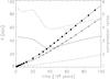Fig. 4 The locations of the two shock fronts (forward shock: filled squares; reverse shock: open diamonds) for galactic distances z ≤ 100   kpc and compression ratios of the gas as a function of time. Already at early times (t ≤ 20  ×  106years) the shock propagation almost becomes constant. The solid line denotes the compression ratio of the forward gas subshock, the dashed line depicts the total compression ratio including the contribution form the cosmic ray precursor. The dashed-dotted line plots the gas compression ratio of the reverse shock growing in time (see text for more details).

The cosmic ray pressure (Fig. 3d) dominates the flow structure as can be easily inferred by comparison with the gas pressure of panel c. Energetic particles contributing to the cosmic ray pressure are mainly accelerated at the forward shock, and the shock structure is smoothed when the precursor region develops. Since we have adopted a mean cosmic ray diffusion coefficient of the typical acceleration time scale yields $\mathit{\tau }\mathrm{~}\mathit{\kappa ̅}\mathit{/}{\mathit{u}}_{\mathrm{s}}^{\mathrm{2}}\mathrm{~}\mathrm{1.5}\mathrm{\times }{\mathrm{10}}^{\mathrm{6}}\hspace{0.17em}$years for an initial shock velocity of 450   km   s^-1. The spatial scale corresponding to this acceleration time is given by , which is very close to the inner boundary. As also discussed in Sect. 4 and depicted in Fig. 7 the particles are accelerated rapidly and close to the galactic plane. Although the reverse shock does not play an important rôle for the overall cosmic ray pressure at the early outflow stages (see also Fig. 4) a small number of individual particles will gain additional energy from this second shock wave (see also Fig. 7).

In Fig. 3d we have also plotted the radial variations in the wave pressure P_w by dashed lines, where the corresponding wave energy Eq. (5) contains the dissipation term v_A∇P_c heating the thermal gas. The typical shape of these curves clearly exhibits the location of the forward and the reverse shocks, seen as pronounced changes of P_w. We can also infer the importance of particle acceleration by the smoothed edges. Again, the wind parameters typical of our Milky way show the importance of the excited MHD-fluctuations P_w =  ⟨ (δB)² ⟩ /8π with P_w = (γ_w − 1)E_w and γ_w = 3/2 for driving the outflow. Without the additional diffusive transport due to acting on the cosmic ray pressure P_c the wave pressure P_w is largely affected by the reverse shock seen, e.g., at z = 73   kpc for the rightmost plotted time of t = 1.0 × 10⁸   years. Within the zone of the two shock waves the wave pressure P_w remains above the thermal pressure P_g. However, we do not want to stretch this argument any further, because some care must be applied to the importance of wave pressure. As mentioned before, nonlinear Landau damping will limit wave growth severely, resulting in additional thermal heating of the plasma.

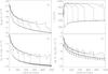Fig. 5 The time-dependent flow structure of a galactic wind up to 1   Mpc at seven different times at 3.7 × 107, 1.1 × 108, 2.3 × 108, 3.7 × 108, 5.3 × 108, 7.7 × 108, and 1.0 × 109   years. At t = 0 the gas and cosmic ray pressure has been increased by a factor of 10 at the inner boundary of the flux tube, simulating a series of violent SN-explosions within a short time interval. In Panel a) the development of the density structure is plotted, where both the forward and the reverse shocks become visible. The velocity in  [km   s-1]  is depicted in panel b) where the particle acceleration broadens the shock fronts in time. In panels c) and d) the curves correspond to the gas and the cosmic ray pressure, together with the wave pressure (dashed lines), respectively. The velocities of the propagating features are also plotted in Figs. 4 and 6 (see text for more details).

Since the development of shock waves plays an important rôle in re-accelerating the existing population of Galactic cosmic rays (see Sect. 4), we explored the propagation of these flow features in Fig. 4 within the first 10⁸   years after our initial pressure increase at the inner boundary simulating multiple SN explosions. After the initial change, the inner boundary conditions are kept constant, causing nonlinear waves moving outwards at different speeds, leading to a growing separation between the flow features as can be seen in Fig. 4. The velocities can be directly estimated from the slopes and are given in the reference frame of the galaxy and reach 930   km   s^-1 for the forward shock, and 840   km   s^-1 for the reverse shock, respectively. Unlike the solar or the galactic wind, where the termination shock is almost stationary with respect to the source frame, or in a supernova remnant, where the reverse shock is moving inwards thereby heating the ejecta, the reverse shock here is largely convected outwards by the galactic wind flow. In other words, its relative velocity with respect to the contact discontinuity (~80 km s^-1) is much too low compared to the galactic wind speed of  ~900 km s^-1, to propagate back to the disk. This is a direct consequence of the density profile in the undisturbed galactic wind medium, falling off as 1/z² as we shall see. The shock velocities are constant, which can be easily understood in the framework of similarity solutions. If we disregard any processes containing explicit length and time scales during the formation of the flow, the propagation of a fluid element in an ambient medium with density decreasing by a power-law, ρ ∝ z^β, is similar to a stellar wind type flow, in which the outer shock travels a distance ${\mathit{R}}_{\mathrm{s}}\mathrm{\propto }{\mathit{t}}^{\frac{\mathrm{3}}{\mathrm{5}\mathrm{+}\mathit{\beta }}}$. Since for an SN or starburst driven outflow, the terminal wind speed is reached very quickly, and therefore the steady-state wind density behaves as ρ_w ∝ (u_wA(z))^-1, where A(z) is given by Eq. (7). At some distance from the plane, A(z) ∝ z², therefore β =  −2, and thus R_s ∝ t or the shock velocity u_s = dR_s/dt ~ const., clearly visible after t ≳ 2 × 10⁷   years or z ≳ 12   kpc for our Milky Way parameter in Fig. 4 (filled squares). The same must be true for the reverse shock (open squares in Fig. 4), which sees a constantly decreasing density profile, again  ∝ 1/z², as it tries to propagate inwards, but is effectively convected outwards. This is also, by the way, the reason the reverse shock remains strong for a long time (~10⁸   )years, because it does not run into medium with increasing density, where it would have to compress and set an increasing amount of mass into motion. However, the diffusive transport of cosmic rays, as well as the dissipative heating of the thermal gas is important during the early expansion phases and the strength of the reverse shock is therefore best visible in the wave pressure (Fig. 3d, dashed lines). This means that the reverse shock also remains a site of efficient particle acceleration, although particle escape would be primarily away from the galaxy similar to the galactic wind termination shock.

The solid line in Fig. 4 represents the compression ratio of the gas subshock within the forward shock (filled squares), also visible in Fig. 3a. The shock structure also exhibits a cosmic ray precursor where the cosmic rays diffuse ahead of the wave thereby reducing the incoming plasma speed and converting adiabatically the kinetic energy into particle pressure. The thermal gas is compressed in this precursor region, and the overall compression ratio, including this effect, is plotted in the dashed curve of Fig. 4, leading to compression ratios in excess of 4. The variation in the compression ratios is due to the changing background of the initial flow structure (cf. Fig. 1, dotted lines), which is basically confined to the innermost 50   kpc. The dashed-dotted line depicts the gas compression ratio of the reverse shock, which increases in time, since the wind velocity at the inner boundary rises, and the flow has to be decelerated to the almost constant post shock velocity of the forward shock. We emphasize that both shock waves travel at different speeds, as summarized in Table 1, and that the most energetic particles can pick up the various velocity differences to get reaccelerated (see also Fig. 7).

In Fig. 5 the variables are plotted between the inner boundary at 1   kpc and the outer boundary located at 1000   kpc at seven different times. The first time step depicted corresponds to 3.6 × 10⁷   years, followed by 1.1 × 10⁸, 2.3 × 10⁸, 3.7 × 10⁸, 5.3 × 10⁸, 7.7 × 10⁸, and 1.03 × 10⁹   years. The density, velocity, and pressure structures in Fig. 5 clearly exhibit both shock waves and the contact discontinuity, which is more difficult to localize, since several pressure contributions are important within this zone. The slowdown of the gas velocity of about 100   km   s^-1 is caused by the smoothed reverse shock (Fig. 5b). Both shock waves energize cosmic rays and in particular the further acceleration of particles at the reverse shock is clearly visible through the local maxima in the corresponding P_w-curves of Fig. 5d. The increase in the particle pressure, as well as the wave pressure (dashed lines) reveals that the reverse shock remains a site of efficient particle acceleration. Since after t ≳ 1.4 × 10⁷   years, the reverse shock has reached a distance of more than 100   kpc, the particles would tend to move away from the galaxy as at the galactic wind termination shock.

In the forward shock the outflowing gas is pushed from 400   km   s^-1 to 800   km   s^-1. Consequently, the overall flow time through the wind up to 1   Mpc is shortened from the initial model of 3.2  ×  10⁹   years to 1.08 × 10⁹   years corresponding to a factor of 3. The latter timespan is also identical to the time the initial perturbation needs to travel to the outer boundary located at 1   Mpc.

4. Particle acceleration in galactic winds

As seen in the previous section, a temporal variation due to changes in the star formation rate (and hence SN-rate) leads to an increase in the gas pressure at the bottom of a flux tube. Such time-dependent boundary conditions at the reference level result almost inevitably in (several) shock waves propagating into the halo (and possibly coalescing) as outlined in the previous section. Under such conditions (two shock waves separated by a contact discontinuity, cf. Fig. 5) energetic particles can gain energy through the first-order Fermi-mechanism. The bulk of the particles, which enter the diffusive shock acceleration process, are already energized CRs from the disk sources so that there is no need to worry about injection. These particles instead undergo a reacceleration process. In contrast to the compression waves of the “slipping interaction regions” discussed in Völk & Zirakashvili (2004), the shock waves considered here can be strong. Since both forward and reverse shocks are running down a density gradient, they can strengthen considerably already close to the disk (see Fig. 5).

Diffusive particle transport along the magnetic field lines of the flux tube in the time-dependent galactic wind flow thus opens the possibility to accelerate cosmic rays to energies well beyond the knee, if large-scale shock waves propagate through the wind. Adopting for simplicity the test particle picture (e.g. Drury 1983) we can integrate the equation $\frac{\mathrm{d}{\mathit{p}}_{\max }}{\mathrm{d}\mathit{t}}\mathrm{=}\frac{{\mathit{p}}_{\max }}{{\mathit{\tau }}_{\mathrm{acc}}}$(12)to estimate the maximum momentum p_max reached during the life time of a shock wave. We use the particle momentum in units of mc. The diffusive acceleration time scale at a shock wave with upstream velocity u₁ and downstream velocity u₂ for a planar shock (the radius of curvature is much larger than for supernova remnants) is given by ${\mathit{\tau }}_{\mathrm{acc}}\mathrm{=}\frac{\mathrm{3}}{{\mathit{u}}_{\mathrm{1}}\mathrm{-}{\mathit{u}}_{\mathrm{2}}}\left(\frac{{\mathit{\kappa }}_{\mathrm{1}}}{{\mathit{u}}_{\mathrm{1}}}\mathrm{+}\frac{{\mathit{\kappa }}_{\mathrm{2}}}{{\mathit{u}}_{\mathrm{2}}}\right)\mathrm{·}$(13)The diffusion coefficients κ_1,2 = κ(p) depend on the particle momentum p. If fully developed turbulence is assumed the so-called Bohm limit, where the mean free path is essentially reduced to a particle gyroradius, can be adopted, and for a particle with mass m and charge Ze the diffusion coefficient reads as 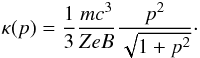$\mathit{\kappa }\mathrm{\left(}\mathit{p}\mathrm{\right)}\mathrm{=}\frac{\mathrm{1}}{\mathrm{3}}\frac{\mathit{m}{\mathit{c}}^{\mathrm{3}}}{\mathit{ZeB}}\frac{{\mathit{p}}^{\mathrm{2}}}{\sqrt{\mathrm{1}\mathrm{+}{\mathit{p}}^{\mathrm{2}}}}\mathrm{·}$(14)The Bohm limit means that the field is completely random on a scale of the order of the gyroradius, and thus represents a minimum diffusion coefficient. It is indeed questionable whether higher energy particles find a wave field, which is random enough on larger scales for strong scattering to still be applicable (Dogiel et al. 1994). On the other hand, in some models for accelerating CRs beyond the knee (Lucek & Bell 2000; Bell & Lucek 2001), it has been argued that while downstream of a shock wave, strong turbulence is excited and isotropization of the CR distribution function is rapid enough to promote recrossing, also nonlinear field amplification by CRs can occur upstream (see also McKenzie & Völk 1982). Nonetheless, in our numerical calculations, we also have taken larger diffusion coefficients into account. As CR streaming generates waves for resonant interaction, it has been suggested to assume that there is still a sufficient number of waves excited to guarantee pitch angle scattering, hence the validity of the first-order Fermi acceleration process. As seen in the previous formula, the magnetic field strength B enters through the diffusion coefficient κ(p), and according to ∇·B = 0, the adopted flux tube geometry (Eq. (7)) implies $\mathit{A}\mathrm{\left(}\mathit{z}\mathrm{\right)}\mathit{B}\mathrm{\left(}\mathit{z}\mathrm{\right)}\mathrm{=}{\mathit{A}}_{\mathrm{0}}{\mathit{B}}_{\mathrm{0}}\mathit{,} \mathit{B}\mathrm{\left(}\mathit{z}\mathrm{\right)}\mathrm{=}{\mathit{B}}_{\mathrm{0}}\hspace{0.17em}{\left[\mathrm{1}\mathrm{+}{\left(\frac{\mathit{z}}{{\mathit{z}}_{\mathrm{0}}}\right)}^{\mathrm{2}}\right]}^{-1}\mathit{.}$(15)As the flow and the shocks in a flux tube are propagating along the magnetic field, we are dealing with parallel shocks here with no field compression. It has been suggested though that the maximum energy gained by diffusive shock acceleration is higher for perpendicular shocks, when κ is small, provided diffusion across the shock is fast enough to allow for multiple shock crossings (e.g. Jokipii 1987).

Fig. 6 The various velocities occurring in the time-dependent solutions also plotted in Fig. 5 as a function of time. All velocities are given in the rest frame of the galaxy. The solid line depicts the velocity of the forward shock vs and the dashed line the reverse shock vr. The highest gas velocity (filled squares) gives the upstream velocity of the reverse shock v2. The open triangles plot the post shock velocity v1 of the reverse shock. The open diamonds correspond to the gas velocity v0 three diffusive scales in front of the forward shock. In less than about 7 × 107   years or r < 50   kpc, all the velocities become constant and are also given in Table 1.

It is straightforward to understand the acceleration characteristics, if we take a look at sufficiently large time scales t ≫ t₀ and therefore z ≫ z₀. As seen in Fig. 6 the discontinuities are propagating at constant velocities, so that we can write, e.g., the distance of a shock from the galactic plane as z = u_st, where u_s denotes the shock velocity as given in Table 1. As a result, Eq. (14) reduces via Eq. (15) for large z ≫ z₀ and p ≫ 1 to $\mathit{\kappa }\mathrm{\left(}\mathit{p}\mathrm{\right)}\mathrm{\simeq }\frac{\mathrm{1}}{\mathrm{3}}\frac{\mathit{m}{\mathit{c}}^{\mathrm{3}}}{\mathit{Ze}{\mathit{B}}_{\mathrm{0}}{\mathit{z}}_{\mathrm{0}}^{\mathrm{2}}}\hspace{0.17em}{\mathit{u}}_{\mathrm{s}}^{\mathrm{2}}{\mathit{t}}^{\mathrm{2}}\mathit{p}\mathit{.}$(16)Approximating also ${\mathit{\tau }}_{\mathrm{acc}}\mathrm{\simeq }\mathrm{4}\mathit{\kappa }\mathrm{\left(}\mathit{p}\mathrm{\right)}\mathit{/}{\mathit{u}}_{\mathrm{s}}^{\mathrm{2}}$ we end up with a simplified equation for the maximum momentum p_max valid for the long term evolution $\frac{\mathrm{d}{\mathit{p}}_{\max }}{\mathrm{d}\mathit{t}}\mathrm{=}\frac{\mathit{A}}{{\mathit{t}}^{\mathrm{2}}}\mathit{,} \mathit{A}\mathrm{=}\frac{\mathrm{3}\mathit{Ze}{\mathit{B}}_{\mathrm{0}}{\mathit{z}}_{\mathrm{0}}^{\mathrm{2}}}{\mathrm{4}\mathit{m}{\mathit{c}}^{\mathrm{3}}}\mathrm{·}$(17)This equation can be integrated easily, and specifying the initial conditions by p(t₀) = p₀ at some time t₀, we get for t ≥ t₀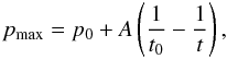${\mathit{p}}_{\max }\mathrm{=}{\mathit{p}}_{\mathrm{0}}\mathrm{+}\mathit{A}\left(\frac{\mathrm{1}}{{\mathit{t}}_{\mathrm{0}}}\mathrm{-}\frac{\mathrm{1}}{\mathit{t}}\right)\mathit{,}$(18)which leads to an almost constant maximum momentum p_max after the initial acceleration.

This behavior of p_max is clearly visible in Fig. 7 where Eq. (12) has been integrated in time for our velocity jumps. After the initial phase of a few 10⁶   years the momentum remains almost constant in accordance with the analytical estimate of Eq. (18). As plotted in Figs. 3 and 5, the structure of the time-dependent flow exhibits two shock waves, and energetic particles can be (re)accelerated at both shock waves. The two curves depict the differences between the cases of one and two shocks. The full squares show the maximum momentum of particles if only the acceleration at the forward shock is considered; i.e., only the forward shock velocities u₁ and u₂ are used in Eq. (13). The upper curve reaching even a higher particle momentum is computed by using the velocity difference between the upstream region of the forward shock and the downstream region of the reverse shock. The acceleration at both shocks can therefore increase the maximum momentum by another factor of two compared to the acceleration only at the forward shock. From Fig. 7 it is evident that this reacceleration of energetic particles is very rapid and occurs early on within a few kpc above the galactic plane.

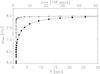Fig. 7 The maximum momentum pmax in units of  [mc]  reached by a cosmic ray particle as a function of the shock distance Rs in  [kpc]  or time in  [106]    years. Already within a few kpc from the galactic plane (corresponding to a flow time of about 107   years) an almost constant particle momentum is achieved. The squares are calculated due to particle acceleration occurring only at the forward shock, and the diamonds also include the acceleration at the reverse shock.

Since particle acceleration here is essentially a first-order Fermi process, we expect the usual power-law spectrum to emerge. It is known from simple one-dimensional diffusive shock acceleration theory for steady plane shocks that for particles injected at some momentum p₀, i.e. for a monoenergetic distribution function, a power-law distribution for the downstream spectrum, f₂(p), will naturally arise, owing to the stochastic nature of the process, such that ${\mathit{f}}_{\mathrm{2}}\mathrm{\left(}\mathit{p}\mathrm{\right)}\mathrm{=}\frac{{\mathit{N}}_{\mathrm{0}}}{\mathrm{4}\mathit{\pi }}\frac{\mathrm{3}{\mathit{u}}_{\mathrm{1}}}{{\mathit{u}}_{\mathrm{1}}\mathrm{-}{\mathit{u}}_{\mathrm{2}}}{\left(\frac{\mathit{p}}{{\mathit{p}}_{\mathrm{0}}}\right)}^{\frac{\mathrm{3}{\mathit{u}}_{\mathrm{1}}}{{\mathit{u}}_{\mathrm{1}}\mathrm{-}{\mathit{u}}_{\mathrm{2}}}}\hspace{0.17em}\mathit{,}$(19)where N₀ is the upstream particle number density with momentum p ≤ p₀. The upstream and downstream velocities u_1,2 measured in the shock frame are given by $\begin{array}{ccc}{\mathit{u}}_{\mathrm{1}}& \mathrm{=}& {\mathit{u}}_{\mathrm{s}}\left(\mathrm{1}\mathrm{-}\frac{{\mathit{u}}_{\mathrm{w}}}{{\mathit{u}}_{\mathrm{s}}}\right)\\ {\mathit{u}}_{\mathrm{2}}& \mathrm{=}& \frac{{\mathit{u}}_{\mathrm{1}}}{\mathit{r}}\hspace{0.17em}\mathit{,}\end{array}$with u_w the undisturbed wind speed, and r the compression ratio. The power-law index in Eq. (19) for a unmodified shock, i.e. in one where the back-reaction of the particles on the shock structure can be still neglected, is then 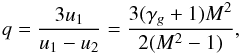$\mathit{q}\mathrm{=}\frac{\mathrm{3}{\mathit{u}}_{\mathrm{1}}}{{\mathit{u}}_{\mathrm{1}}\mathrm{-}{\mathit{u}}_{\mathrm{2}}}\mathrm{=}\frac{\mathrm{3}\mathrm{(}{\mathit{\gamma }}_{\mathit{g}}\mathrm{+}\mathrm{1}\mathrm{)}{\mathit{M}}^{\mathrm{2}}}{\mathrm{2}\mathrm{(}{\mathit{M}}^{\mathrm{2}}\mathrm{-}\mathrm{1}\mathrm{)}}\mathit{,}$(22)where the upstream Mach number is given by 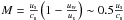$\mathit{M}\mathrm{=}\frac{{\mathit{u}}_{\mathrm{s}}}{{\mathit{c}}_{\mathrm{s}}}{}^{\mathrm{(}}\mathrm{1}\mathrm{-}{\frac{{\mathit{u}}_{\mathrm{w}}}{{\mathit{u}}_{\mathrm{s}}}}^{\mathrm{)}}\mathrm{~}\mathrm{0.5}\frac{{\mathit{u}}_{\mathrm{s}}}{{\mathit{c}}_{\mathrm{s}}}$, for our standard case of z₀ = 15   kpc (see also Table 1); here c_s is the local speed of sound ahead of the shock front. The galactic wind is already highly supersonic near the disk, but the Mach number depends on the relative velocity between the shock and the wind, and only if the flow, which is catching up, is much faster than the quiescent wind, can we expect a strong gas shock and q ≈ 4 during the first 20 million years. However, the compression ratio of the forward shock is r ~ 3 (see Fig. 4), implying q = 4.5, which results in an energy spectral index of α ~ 2.9, including an energy dependent diffusion  ∝ E^-0.65 of the particles propagating back to the disk. A mixture with CRs accelerated by the reverse shock with a lower compression ratio will tend to steepen the spectrum somewhat, which is already quite close to the observed value beyond the “knee”. Since the injected particles are those coming from the disk, and already having a power-law spectrum, the resulting spectrum will also be a power-law. The spectral details will be the subject of further discussion in a forthcoming paper.

5. Discussion and conclusions

Soon after the diffusive shock acceleration theory was established as a major candidate to explain the origin of cosmic rays (Krymsky 1977; Axford et al. 1977; Bell 1978a,b; Blandford & Ostriker 1978), it became clear that supernova shock waves, which are the only non-exotic source of sufficient energy to provide the overall CR flux, would cut off in energy at about 10¹⁴ eV (Lagage & Cesarsky 1983), due to finite lifetime and curvature of the shock. A more recent analysis shows that energies up to Z × 10¹⁵   eV are possible, if diffusion is at the Bohm limit (Berezhko 1996). The observed spectrum between the so-called knee and ankle thus have remained unexplained for a long time. Recent X-ray observations of Tycho’s SNR (Eriksen et al. 2011) are interpreted such that particles are indeed accelerated up to the “knee” in regions of enhanced magnetic turbulence corresponding to particles energies in the range of 10¹⁴   eV. However, the physical process of explaining energies of particles beyond the “knee" up to the “ankle” still remains unclear. We have already mentioned the problems of detecting particles accelerated at the galactic wind termination shock. As discussed previously, several interesting suggestions have been put forward recently to explain the spectrum between the “ankle” and the “knee”. Lucek & Bell (2000) picked up on an earlier idea (e.g., Völk & McKenzie 1981), arguing that the cosmic ray streaming itself would create sufficient turbulence upstream of the shock due to the rapid nonlinear growth of waves. If the SNR shock expanded into a stellar wind cavity, a maximum energy of  ~Z × 10¹⁸   eV (Bell & Lucek 2001) could be achieved, beyond which CRs are commonly believed to be of extragalactic origin.

This hypothesis has received support in Drury et al. (2003). They actually calculated the resulting spectra from a Sedov-type shock in the framework of a simple “box” model, in which the energetic particles are distributed uniformly within one diffusion length across the discontinuity, and are accelerated in momentum directly at the shock. They find a power-law spectrum with a small break at the knee all the way up to the ankle. The magnitude of the break, however, depends on the diffusion length and on scales up- and downstream of the shock. It is therefore not well determined in such a simple model. The break occurs at the correct energy (where ordinary SNR shocks cease to accelerate), but the power-law exponent in the momentum distribution function can vary at the extreme between  − 3.5 (corresponding even to a hardening) and  − 5.75, while observations point to about  − 4.5. Therefore more detailed and presumably numerical calculations are needed in order to quantify the implications of this model. Referring to the self-consistent Galactic CR propagation model by Ptuskin et al. (1997), Völk & Zirakashvili (2004) have questioned the suggestion by Bell & Lucek (2001). They argue that the transition boundary between diffusion and advection will have reached the termination shock at a distance of  ~300   kpc for particles with energies of  ~10¹⁶Z   eV and that particles with higher rigidities diffuse freely upstream of the termination shock and can only escape convectively downstream because of the small diffusion coefficient there, with no change in momentum. Thus the spectrum would be the same as the source spectrum in the disk, corresponding to a hardening of the E^-2.7-spectrum in the halo. In our model, acceleration occurs close to the disk, where the compression ratio is  ~3, making the spectrum naturally steeper near the sources than in the disk. In addition, the particles have to diffuse back to the disk, leading to further steepening of the spectrum, as discussed in the previous section. A detailed discussion of this problem will be presented in a sequel paper. Here we would just like to emphasize that time-dependent changes in the boundary conditions of the galactic wind, naturally lead to the formation of strong shocks that will reaccelerate particles to energies well above the knee. We agree with Völk & Zirakashvili (2004) that the analysis of the cosmic ray spectrum has to include the propagation effects of particles not only in the disk, but also in the Galactic halo. While we have analyzed these effects for starburst regions, it is clear that a similar scenario must hold for our Galaxy, although presumably restricted to smaller regions in the underlying Galactic disk. Nevertheless, 3D numerical simulations by Avillez & Breitschwerdt (2004) have shown that outflow occurs even for thick Lockman and Reynolds type gas disks. The crucial point is that once overpressured hot regions have punched a hole in the lower halo, material can travel almost unimpeded to considerable heights, resulting in an outflow once the cosmic ray pressure gradient takes over. These outflows will be modulated in a similar manner as the starburst types, due to changes in the star formation rate. The resulting shock waves can also be strong, because as we have emphasized, it is the relative velocity between fast and slow winds that matters, and steepening of the shock wave will occur as it runs down the galactic wind density gradient.

In addition to the dynamical phenomena caused by SN-explosions, the magnetic field may also cause changes in the dynamics of the flow, and the idealized geometry will only approximate reality on average and on large scales. On smaller scales the field geometry can be quite complex, as shown by 3D numerical MHD simulations (e.g. Korpi et al. 1999; Avillez & Breitschwerdt 2005). The tangling of field lines will inevitably lead to a change in topology by magnetic reconnection (Parker 1992) and to additional heating. Also MHD wave heating of the halo has been considered to be responsible for highly ionized species (Hartquist 1983). Field diffusivity and turbulence, which are a natural consequence of a SN-driven ISM (Avillez & Breitschwerdt 2005), will further promote dynamo action and B-field amplification (e.g. Gressel et al. 2008). Magnetized winds in other galaxies, e.g. dwarf galaxies, have also been modeled (Dubois & Teyssier 2010) in order to study the enrichment of the intergalactic medium with magnetic fields within a cosmological context.

Our model treats the base of the halo as an inner boundary condition, from which the flow emanates. In reality, there is a transition between disk and halo, and the outflow is a consequence of time-dependent SN activity in the disk. Again, a 3D numerical simulation would be necessary to properly model fountain flows (e.g. Avillez & Breitschwerdt 2004). However, none of the 3D models put forward so far has considered the effect of CRs and their nonlinear coupling to the flow, which is the purpose of this analysis.

Although also neglecting effects of Galactic rotation and nonlinear wave damping, our model has the advantage that particle acceleration is calculated self-consistently along with the galactic wind flow. The hydrodynamic version of the transport equation that we use even allows us to enter the nonlinear regime, where the shocks can be modified by the increasing CR pressure, so we are not restricted to test particle arguments. Such a self-consistent picture allows us not only to deduce interesting quantities like mass-loss rate of a galaxy, but also to calculate e.g. X-ray spectra that can be compared to XMM-Newton and Chandra observations, in particular for delayed recombination from nonequilibrium distributions of ions in the halo (cf. Breitschwerdt 2003). In a next step we will include the CR momentum distribution function to numerically calculate the resulting cosmic ray spectra between the “knee” and the “ankle”.

To summarize, in this paper we have shown that

• 1.

  time-dependent galactic winds have an asymptotic behaviorthat matches the steady-state solutions obtained byBreitschwerdt et al. (1991) verywell;

• 2.

  these steady-state solutions are stable with respect to perturbations;

• 3.

  changes in the inner boundary conditions are very likely to occur, since the flow time of the wind gas is on the order of 10⁸ years, so much longer than the switch-on time for superbubbles or starbursts;

• 4.

  changes in the boundary conditions, in particular an increase in pressure due to increased star formation rate, result in time-dependent features like shocks (forward and reverse) and contact discontinuities;

• 5.

  these shocks running down a density gradient can become very strong and propagate with roughly constant velocity;

• 6.

  cosmic rays, propagating along with outflowing gas from the disk, can be accelerated very efficiently to energies up to 10¹⁷−10¹⁸Z   eV by these shocks, thus suggesting a new mechanism for generating the Galactic cosmic rays between the “knee” and the “ankle”;

• 7.

  particle acceleration is very fast and occurs close to the galactic disk, typically with a few kpc;

• 8.

  the particle spectrum at the shock is most likely steeper than in the disk, because the Mach number of the forward shock depends on the relative velocity between the background wind and compressional waves, and is therefore smaller. This leads to a spectral index  <−4, i.e. a steepening at the shock. In particular, in the Milky Way, where bursts of star formation are less violent, shocks forming in the halo will have lower Mach numbers, thus leading to a steepening of a spectrum beyond the “knee”;

• 9.

  in addition the spectrum must also steepen, because the particles have to diffuse back to the disk; thus, the lower galactic halo seems to be a promising site for accelerating CRs beyond the “knee”.

Acknowledgments

Part of this work has been supported by the Jubiläumsfonds der Oesterreichischen Nationalbank under project number 4605. The publication is supported by the Austrian Science Fund (FWF). D.B. acknowledges support from the Bundesministerium für Bildung und Forschung (BMBF) by the Deutsches Zentrum für Luft- und Raumfahrt (DLR) under grant 50 OR 0207 and the Max-Planck-Gesellschaft (MPG), where part of this work was already carried out.

References

Appendix A: Discretized equations

The system of equations presented in Sect. 2.1 are rewritten to an integral form, which is necessary for applying a finite volume discretization. Following this procedure ensures the numerical conservation of mass, momentum, and energy.

Introducing the temporal operator by δx = x − x^old between the two time levels t = t^old + δt, as well as the spatial difference Δx_l = x_l + 1 − x_l, we get a discrete version of the corresponding physical Eqs. (1)–(5). By defining the discrete volume between the distances z_l and z_l + 1 through 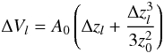$\mathrm{\Delta }{\mathit{V}}_{\mathit{l}}\mathrm{=}{\mathit{A}}_{\mathrm{0}}\left(\mathrm{\Delta }{\mathit{z}}_{\mathit{l}}\mathrm{+}\frac{\mathrm{\Delta }{\mathit{z}}_{\mathit{l}}^{\mathrm{3}}}{\mathrm{3}{\mathit{z}}_{\mathrm{0}}^{\mathrm{2}}}\right)$(A.1)we get, e.g., 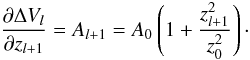$\frac{\mathit{\partial }\mathrm{\Delta }{\mathit{V}}_{\mathit{l}}}{\mathit{\partial }{\mathit{z}}_{\mathit{l}\mathrm{+}\mathrm{1}}}\mathrm{=}{\mathit{A}}_{\mathit{l}\mathrm{+}\mathrm{1}}\mathrm{=}{\mathit{A}}_{\mathrm{0}}\left(\mathrm{1}\mathrm{+}\frac{{\mathit{z}}_{\mathit{l}\mathrm{+}\mathrm{1}}^{\mathrm{2}}}{{\mathit{z}}_{\mathrm{0}}^{\mathrm{2}}}\right)\mathrm{·}$(A.2)Since the adaptive grid changes the locations of grid points, we have to compute the relative velocity 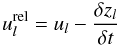${\mathit{u}}_{\mathit{l}}^{\mathrm{rel}}\mathrm{=}{\mathit{u}}_{\mathit{l}}\mathrm{-}\frac{\mathit{\delta }{\mathit{z}}_{\mathit{l}}}{\mathit{\delta t}}$(A.3)with respect to the grid motion and u^rel appears in all advection terms.

Written in a conservation form for a the flux-tube geometry, the discrete equation of continuity (1) reads as 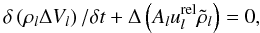$\mathit{\delta }\left({\mathit{\rho }}_{\mathit{l}}\mathrm{\Delta }{\mathit{V}}_{\mathit{l}}\right)\mathit{/}\mathit{\delta t}\mathrm{+}\mathrm{\Delta }\mathrm{(}{\mathit{A}}_{\mathit{l}}{\mathit{u}}_{\mathit{l}}^{\mathrm{rel}}{\begin{array}{}\mathrm{˜}\\ {\mathit{\rho }}_{\mathit{l}}\end{array}}^{\mathrm{)}}\mathrm{=}\mathrm{0}\mathit{,}$(A.4)where $\begin{array}{}{\mathrm{˜}}_{}\\ {\mathit{\rho }}_{\mathit{l}}\end{array}$ denotes the density upstream to the relative velocity ${\mathit{u}}_{\mathit{l}}^{\mathrm{rel}}$. Owing to the mathematical properties of hyperbolic conservation laws, only those discretization schemes are stable that take the direction of the flow into account (see e.g. LeVeque 1990 for all mathematical details). The equation of motion (2) is given by 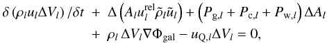$\begin{array}{ccc}\mathit{\delta }\left({\mathit{\rho }}_{\mathit{l}}{\mathit{u}}_{\mathit{l}}\mathrm{\Delta }{\mathit{V}}_{\mathit{l}}\right)\mathit{/}\mathit{\delta t}& \mathrm{+}& \mathrm{\Delta }\mathrm{(}{\mathit{A}}_{\mathit{l}}{\mathit{u}}_{\mathit{l}}^{\mathrm{rel}}\begin{array}{}\mathrm{˜}\\ {\mathit{\rho }}_{\mathit{l}}\end{array}{\begin{array}{}\mathrm{˜}\\ {\mathit{u}}_{\mathit{l}}\end{array}}^{\mathrm{)}}\mathrm{+}\mathrm{(}{\mathit{P}}_{\mathrm{g}\mathit{,l}}\mathrm{+}{\mathit{P}}_{\mathrm{c}\mathit{,l}}\mathrm{+}{\mathit{P}}_{\mathrm{w}\mathit{,l}}\mathrm{)}\mathrm{\Delta }{\mathit{A}}_{\mathit{l}}\\ & \mathrm{+}& {\mathit{\rho }}_{\mathit{l}}\hspace{0.17em}\mathrm{\Delta }{\mathit{V}}_{\mathit{l}}\mathrm{\nabla }{\mathrm{\Phi }}_{\mathrm{gal}}\mathrm{-}{\mathit{u}}_{\mathrm{Q}\mathit{,l}}\mathrm{\Delta }{\mathit{V}}_{\mathit{l}}\mathrm{=}\mathrm{0}\mathit{,}\end{array}$(A.5)where u_Q,l stands for the artificial pressure term added to broaden shock fronts over a finite length scale, typically l_q = 10^-3z. The gas energy density (3) reads in the volume-integrated discrete form 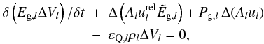$\begin{array}{ccc}\mathit{\delta }\mathrm{(}{\mathit{E}}_{\mathrm{g}\mathit{,l}}\mathrm{\Delta }{\mathit{V}}_{\mathit{l}}\mathrm{)}\mathit{/}\mathit{\delta t}& \mathrm{+}& \mathrm{\Delta }\mathrm{(}{\mathit{A}}_{\mathit{l}}{\mathit{u}}_{\mathit{l}}^{\mathrm{rel}}{\begin{array}{}\mathrm{˜}\\ {\mathit{E}}_{\mathrm{g}\mathit{,l}}\end{array}}^{\mathrm{)}}\mathrm{+}{\mathit{P}}_{\mathrm{g}\mathit{,l}}\hspace{0.17em}\mathrm{\Delta }\mathrm{\left(}{\mathit{A}}_{\mathit{l}}{\mathit{u}}_{\mathit{l}}\mathrm{\right)}\\ & \mathrm{-}& {\mathit{\epsilon }}_{\mathrm{Q}\mathit{,l}}{\mathit{\rho }}_{\mathit{l}}\mathrm{\Delta }{\mathit{V}}_{\mathit{l}}\mathrm{=}\mathrm{0}\mathit{,}\end{array}$(A.6)which also includes the viscous energy dissipation term ε_Q. The cosmic ray energy density (4) is given through $\begin{array}{ccc}\mathit{\delta }\left({\mathit{E}}_{\mathrm{c}\mathit{,l}}\mathrm{\Delta }{\mathit{V}}_{\mathit{l}}\right)\mathit{/}\mathit{\delta t}& \mathrm{+}& \mathrm{\Delta }\mathrm{(}{\mathit{A}}_{\mathit{l}}{\mathit{u}}_{\mathit{l}}^{\mathrm{rel}}{\begin{array}{}\mathrm{˜}\\ {\mathit{E}}_{\mathrm{c}\mathit{,l}}\end{array}}^{\mathrm{)}}\\ & \mathrm{+}& \mathrm{(}{\mathit{\gamma }}_{\mathrm{c}}\mathrm{-}\mathrm{1}\mathrm{)}{\mathit{E}}_{\mathrm{c}\mathit{,l}}\hspace{0.17em}\mathrm{\Delta }\mathrm{\left(}{\mathit{A}}_{\mathit{l}}{\mathit{u}}_{\mathit{l}}\mathrm{\right)}\mathrm{=}\mathrm{0.}\end{array}$(A.7)Finally, we have also to solve the equation of wave energy density (5) $\begin{array}{ccc}\mathit{\delta }\left({\mathit{E}}_{\mathrm{w}\mathit{,l}}\mathrm{\Delta }{\mathit{V}}_{\mathit{l}}\right)\mathit{/}\mathit{\delta t}& \mathrm{+}& \mathrm{\Delta }\mathrm{(}{\mathit{A}}_{\mathit{l}}{\mathit{u}}_{\mathit{l}}^{\mathrm{rel}}{\begin{array}{}\mathrm{˜}\\ {\mathit{E}}_{\mathrm{w}\mathit{,l}}\end{array}}^{\mathrm{)}}\\ & \mathrm{+}& \mathrm{(}{\mathit{\gamma }}_{\mathrm{w}}\mathrm{-}\mathrm{1}\mathrm{)}{\mathit{E}}_{\mathrm{w}\mathit{,l}}\hspace{0.17em}\mathrm{\Delta }\mathrm{\left(}{\mathit{A}}_{\mathit{l}}{\mathit{u}}_{\mathit{l}}\mathrm{\right)}\mathrm{=}\mathrm{0.}\end{array}$(A.8)This set of physical equations is augmented by the grid equation, which redistributes the grid points within the computational domain, and all details about this numerical technique can be found in Dorfi & Drury (1987). Therefore, in total we obtain 6N discrete nonlinear algebraic equations for the unknowns ρ_l, u_l, E_g,l, E_c,l, E_w,l, and z_l at every index l, where N = 300 is the number of spatial grid points. The resulting algebraic system is solved at every new time step by adopting a Newton-Raphson iteration procedure where the corresponding Jacobian matrix has to be calculated from the discrete set of Eqs. (A.4)–(A.8).

Due to the implicit nature of our numerical scheme we can compute time-dependent as well as stationary solutions, which can directly be compared to the stationary solutions obtained from solving the ODEs from the time-independent equations (Breitschwerdt et al. 1991). Furthermore, in the steady state case integrals of the equations can be derived and used for a numerical check of the code. Both methods show that the local, as well as global differences between the solution of the ODE system and the numerical scheme presented above are less than 10^-5 everywhere. This small difference remains because of the staggered mesh representation of the physical quantities and the relative accuracy of the Newton-iteration of 10^-6.

Appendix B: Artificial viscosity

Shock fronts are treated by applying an artificial viscosity in tensor form based on the work of Tscharnuter & Winkler (1979). Since we are using an adaptive grid (Dorfi & Drury 1987) the length scale of the broadening l_q can be specified according to our physical needs, i.e. l_q ≪ l_CR = κ/u_s, which defines the length scale due to the particle acceleration. This way we can ensure that particles are accelerated by the 1.-order Fermi mechanism because the shock front is seen as a discontinuity by the energetic particles.

The tensor formulation of the artificial viscosity requires some calculations for the adopted flux tube geometry since the pressure tensor Q, the viscous momentum transfer u_Q and the viscous energy dissipation ε_Q have to be calculated. Without more details (see Tscharnuter & Winkler 1979) we state these quantities $\begin{array}{ccc}{Q}& \mathrm{=}& \\ {\mathit{u}}_{\mathrm{Q}}& \mathrm{=}& \\ {\mathit{\epsilon }}_{\mathrm{Q}}& \mathrm{=}& \end{array}$where (∇u) is the symmetrized velocity gradient and I the unity tensor.

Artificial viscosity coefficient μ_Q consists of a linear and a quadratic term weighted by q₁ and q₂, i.e., ${\mathit{\mu }}_{\mathrm{Q}}\mathrm{=}\mathrm{-}{\mathit{q}}_{\mathrm{1}}{\mathit{l}}_{\mathrm{q}}{\mathit{c}}_{\mathrm{s}}\mathrm{+}{\mathit{q}}_{\mathrm{2}}^{\mathrm{2}}{\mathit{l}}_{\mathrm{q}}^{\mathrm{2}}\begin{array}{}\min \end{array}\mathrm{(}\mathrm{\nabla }\mathrm{·}{u}\mathit{,}\mathrm{0}\mathrm{)}\mathit{.}$(B.4)The definition of μ_Q include a typical viscous length scale l_q. When inspecting the last expression one sees that the linear term in l_q also scales with the sound velocity c_s and is always present when q₁ ≠ 0. The second term is quadratic in l_q, and it is evident that compressive and nonhomologous motions; i.e., ∇·u < 0 and tr(Q) ≠ 0 produce a viscous pressure. The amount of artificial viscosity is then determined by these length scales q₁l_q and q₂l_q.

To obtain the corresponding expressions (B.2) and (B.3) for our flux tube geometry, we recall that the distance from the galactic plane is denoted by z and the area of the flux tube is defined by A(z). Neglecting the curvature within the flux tube area, we get the simple orthogonal metric tensor by ${\mathit{g}}_{\mathit{ik}}\mathrm{=}\left(\begin{array}{c}\\ \mathrm{1}& \mathrm{0}& \mathrm{0}\\ \mathrm{0}& {\mathit{z}}^{\mathrm{2}}& \mathrm{0}\\ \mathrm{0}& \mathrm{0}& {\mathit{A}}^{\mathrm{2}}\end{array}\right)\mathit{.}$(B.5)Following the rules derived by Tscharnuter & Winkler (1979), we can calculate the divergence of the velocity from the last expression $\mathrm{\nabla }\mathrm{·}{u}\mathrm{=}\frac{\mathrm{1}}{\mathit{A}}\frac{\mathit{\partial Au}}{\mathit{\partial z}}\mathrm{=}\frac{\mathit{\partial Au}}{\mathit{\partial V}}\mathit{,}$(B.6)as well as the symmetrized velocity gradient 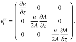${\mathit{ϵ}}_{\mathit{l}}^{\mathit{m}}\mathrm{=}\left(\begin{array}{c}\\ \frac{\mathit{\partial u}}{\mathit{\partial z}}& \mathrm{0}& \mathrm{0}\\ \mathrm{0}& \frac{\mathit{u}}{\mathrm{2}\mathit{A}}\frac{\mathit{\partial A}}{\mathit{\partial z}}& \mathrm{0}\\ \mathrm{0}& \mathrm{0}& \frac{\mathit{u}}{\mathrm{2}\mathit{A}}\frac{\mathit{\partial A}}{\mathit{\partial z}}\end{array}\right)\mathit{.}$(B.7)The viscous pressure tensor is given through 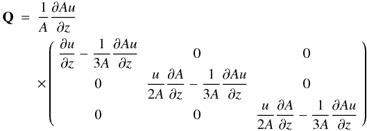$\begin{array}{ccc}{Q}& \mathrm{=}& \frac{\mathrm{1}}{\mathit{A}}\frac{\mathit{\partial Au}}{\mathit{\partial z}}\\ & & \mathrm{\times }\left(\begin{array}{c}\\ & & \\ & & \\ & & \end{array}\right)\end{array}$(B.8)and has the desired property of being traceless; i.e., there is no artificial viscosity in the case of homologous motions. According to the previous terms, the viscous pressure is given in the flux tube geometry through ${\mathit{u}}_{\mathrm{Q}}\mathrm{=}\frac{\mathrm{1}}{{\mathit{A}}^{\mathrm{3}\mathit{/}\mathrm{2}}}\frac{\mathit{\partial }}{\mathit{\partial z}}\left[{\mathit{A}}^{\mathrm{1}\mathit{/}\mathrm{2}}{\mathit{\mu }}_{\mathrm{Q}}\hspace{0.17em}\mathit{\rho }\frac{\mathit{\partial Au}}{\mathit{\partial z}}\left(\frac{\mathit{\partial u}}{\mathit{\partial z}}\mathrm{-}\frac{\mathrm{1}}{\mathrm{3}}\frac{\mathit{\partial Au}}{\mathit{\partial z}}\right)\right]\mathit{.}$(B.9)The energy dissipation by the viscosity is determined from the contraction of the pressure tensor with the symmetrized velocity gradient (see Eq. (B.3)). To ensure physical meaningful results it is necessary to find a discrete version, which always guarantees a positive viscous energy generation. This term has been implemented in our code through ${\mathit{\epsilon }}_{\mathrm{Q}}\mathrm{=}\mathrm{-}\frac{\mathrm{3}}{\mathrm{2}}\frac{{\mathit{\mu }}_{\mathrm{Q}}}{\mathit{A}}\frac{\mathit{\partial Au}}{\mathit{\partial z}}{\left[\frac{\mathit{\partial u}}{\mathit{\partial z}}\mathrm{-}\frac{\mathrm{1}}{\mathrm{3}\mathit{A}}\frac{\mathit{\partial Au}}{\mathit{\partial z}}\right]}^{\mathrm{2}}\mathit{,}$(B.10)guaranteeing that the viscous energy generation ε_Q is also numerically positive.

According to the discretization scheme, the artificial viscosity terms are written as ${\mathit{\mu }}_{\mathrm{Q}\mathit{,l}}\mathrm{=}{\mathit{q}}_{\mathrm{1}}{\mathit{l}}_{\mathrm{q}}\hspace{0.17em}{\mathit{c}}_{\mathrm{s}\mathit{,l}}\mathrm{-}{\mathit{q}}_{\mathrm{2}}{\mathit{l}}_{\mathrm{q}}^{\mathrm{2}}\begin{array}{}\min \end{array}\left(\frac{\mathrm{\Delta }\mathrm{\left(}{\mathit{z}}_{\mathit{l}}^{\mathrm{2}}{\mathit{u}}_{\mathit{l}}\mathrm{\right)}}{\mathrm{\Delta }{\mathit{V}}_{\mathit{l}}}\mathit{,}\hspace{0.17em}\mathrm{0}\right)\mathit{,}$(B.11)including the linear part with c_s,l, the adiabatic sound velocity at a grid point z_l. The corresponding discrete and volume-integrated versions of u_Q and ε_Q are then given as follows. The viscous pressure term in the discrete equation of motion (A.5) reads as $\begin{array}{ccc}{\mathit{u}}_{\mathrm{Q}\mathit{,l}}\mathrm{\Delta }{\mathit{V}}_{\mathit{l}}& \mathrm{=}& \\ & \mathrm{-}& \frac{\mathrm{1}}{\sqrt{{\mathit{A}}_{\mathit{l}}}}\mathrm{\Delta }\left(\mathit{A̅}\begin{array}{}\hspace{0.17em}\mathrm{3}\mathit{/}\mathrm{2}\\ \mathit{l}\end{array}{\mathit{\mu }}_{\mathrm{Q}\mathit{,l}}\hspace{0.17em}{\mathit{\rho }}_{\mathit{l}}\frac{\mathrm{\Delta }\mathrm{\left(}{\mathit{A}}_{\mathit{l}}{\mathit{u}}_{\mathit{l}}\mathrm{\right)}}{\mathrm{\Delta }{\mathit{V}}_{\mathit{l}}}\left[\frac{\mathrm{\Delta }{\mathit{u}}_{\mathit{l}}}{\mathrm{\Delta }{\mathit{z}}_{\mathit{l}}}\mathrm{-}\frac{\mathrm{1}}{\mathrm{3}}\frac{\mathrm{\Delta }\mathrm{\left(}{\mathit{A}}_{\mathit{l}}{\mathit{u}}_{\mathit{l}}\mathrm{\right)}}{\mathrm{\Delta }{\mathit{V}}_{\mathit{l}}}\right]\right)\mathit{,}\end{array}$(B.12)and the corresponding viscous energy dissipation (A.6) is discretized at a grid point z_l according to ${\mathit{\epsilon }}_{\mathrm{Q}\mathit{,l}}{\mathit{\rho }}_{\mathit{l}}\mathrm{\Delta }{\mathit{V}}_{\mathit{l}}\mathrm{=}\frac{\mathrm{3}}{\mathrm{2}}{\mathit{\mu }}_{\mathrm{Q}\mathit{,l}}\hspace{0.17em}{\mathit{\rho }}_{\mathit{l}}\mathrm{\Delta }\mathrm{\left(}\mathrm{\right(}{\mathit{A}}_{\mathit{l}}{\mathit{u}}_{\mathit{l}}\mathrm{\left)}\mathrm{\right)}{\left[\frac{\mathrm{\Delta }{\mathit{u}}_{\mathit{l}}}{\mathrm{\Delta }{\mathit{z}}_{\mathit{l}}}\mathrm{-}\frac{\mathrm{1}}{\mathrm{3}}\frac{\mathrm{\Delta }{\mathit{A}}_{\mathit{l}}{\mathit{u}}_{\mathit{l}}}{\mathrm{\Delta }{\mathit{V}}_{\mathit{l}}}\right]}^{\mathrm{2}}\mathrm{\Delta }{\mathit{V}}_{\mathit{l}}\mathit{.}$(B.13)

All Tables

All Figures

Fig. 1 The time-asymptotic flow structure of a galactic wind up to the innermost 200   kpc with different cosmic ray diffusion coefficients . The case (full line) is almost identical to , and noticeable differences occur only for (dotted line), (dashed line), and (dashed-dotted line). The different panels represent: a) gas density; b) gas velocity; c) thermal gas pressure, d) ratio of gas pressure to cosmic ray pressure.

In the text

Fig. 2 Relative mass-loss rates (filled symbols) Ṁ in units of Ṁ0, the mass-loss rate at , and corresponding terminal velocities (open symbols) in  [km   s-1]  for a flux tube located in our Galaxy at a galactocentric distance of R0 = 10   kpc as a function of the mean cosmic ray diffusion coefficient . Only values of reduce the mass loss rate significantly, but also increase the final wind velocities owing to lower thermal gas ejections (see text for details).

In the text

Fig. 3 The time-dependent flow structure of a galactic wind up to 100   kpc at six different times at 3.4 × 106, 2.0 × 107, 3.6 × 107, 5.4 × 107, 7.7 × 107 and 1.0 × 108   years. At t = 0 the gas and cosmic ray pressure has been increased by a factor of 10 at the inner boundary of the flux tube, simulating a violent SN-explosion. Panel a) plots the development of the density structure where the forward as well as the reverse shock become visible. The velocity in  [km   s-1]  is depicted in panel b) where the particle acceleration broadens the shock fronts in time. In panels c) and d) the curves correspond to the gas and the cosmic ray pressure (solid line) together with the wave pressure (dashed lines), respectively. The velocities of these features are also plotted in Figs. 4 and 6 (see text for more details).

In the text

Fig. 4 The locations of the two shock fronts (forward shock: filled squares; reverse shock: open diamonds) for galactic distances z ≤ 100   kpc and compression ratios of the gas as a function of time. Already at early times (t ≤ 20  ×  106years) the shock propagation almost becomes constant. The solid line denotes the compression ratio of the forward gas subshock, the dashed line depicts the total compression ratio including the contribution form the cosmic ray precursor. The dashed-dotted line plots the gas compression ratio of the reverse shock growing in time (see text for more details).

In the text

Fig. 5 The time-dependent flow structure of a galactic wind up to 1   Mpc at seven different times at 3.7 × 107, 1.1 × 108, 2.3 × 108, 3.7 × 108, 5.3 × 108, 7.7 × 108, and 1.0 × 109   years. At t = 0 the gas and cosmic ray pressure has been increased by a factor of 10 at the inner boundary of the flux tube, simulating a series of violent SN-explosions within a short time interval. In Panel a) the development of the density structure is plotted, where both the forward and the reverse shocks become visible. The velocity in  [km   s-1]  is depicted in panel b) where the particle acceleration broadens the shock fronts in time. In panels c) and d) the curves correspond to the gas and the cosmic ray pressure, together with the wave pressure (dashed lines), respectively. The velocities of the propagating features are also plotted in Figs. 4 and 6 (see text for more details).

In the text

Fig. 6 The various velocities occurring in the time-dependent solutions also plotted in Fig. 5 as a function of time. All velocities are given in the rest frame of the galaxy. The solid line depicts the velocity of the forward shock vs and the dashed line the reverse shock vr. The highest gas velocity (filled squares) gives the upstream velocity of the reverse shock v2. The open triangles plot the post shock velocity v1 of the reverse shock. The open diamonds correspond to the gas velocity v0 three diffusive scales in front of the forward shock. In less than about 7 × 107   years or r < 50   kpc, all the velocities become constant and are also given in Table 1.

In the text

Fig. 7 The maximum momentum pmax in units of  [mc]  reached by a cosmic ray particle as a function of the shock distance Rs in  [kpc]  or time in  [106]    years. Already within a few kpc from the galactic plane (corresponding to a flow time of about 107   years) an almost constant particle momentum is achieved. The squares are calculated due to particle acceleration occurring only at the forward shock, and the diamonds also include the acceleration at the reverse shock.

In the text

References

- Adelberger, K. L., & Steidel, C. C. 2000, ApJ, 544, 218 [NASA ADS] [CrossRef] [Google Scholar]
- Axford, W. I. 1981, Proc. Int. School and Workshop on Plasma Astrophysics, Varenna, ESA SP-161, 425 [Google Scholar]
- Axford, W. I., Leer, E., & Skadron, G. 1977, Proc. 15th Int. Cosmic Ray Conf. (Plodiv) 11, 132 [Google Scholar]
- Bell, A. R. 1978a, MNRAS, 182, 147 [NASA ADS] [CrossRef] [Google Scholar]
- Bell, A. R. 1978b, MNRAS, 182, 443 [NASA ADS] [CrossRef] [Google Scholar]
- Bell, A. R. 1987, MNRAS, 215, 615 [NASA ADS] [Google Scholar]
- Bell, A. R., & Lucek, S. G. 2001, MNRAS, 321, 433 [NASA ADS] [CrossRef] [Google Scholar]
- Berezhko, E. G. 1996, Astropart. Phys. 5, 367 [Google Scholar]
- Berezhko, E. G., Yelshin, V. K., & Ksenofontov, L. T. 1994, Astropart. Phys. 2, 215 [Google Scholar]
- Blandford, R. D. 1988, in Supernova Remnants and the Interstellar Medium, ed. R. S. Roger, & T. L. Landecker (Cambridge: Cambridge Univ. Press), 309 [Google Scholar]
- Blandford, R. D., & Eichler, D. 1987, Phys. Rep., 154, 1 [Google Scholar]
- Blandford, R. D., & Ostriker, J. P. 1978, ApJ, 221, L29 [Google Scholar]
- Bregman, J. N. 1980, ApJ, 236, 577 [NASA ADS] [CrossRef] [Google Scholar]
- Bregman, J. N., Hogg, D. E., & Roberts, M. S. 1992, ApJ, 387, 484 [NASA ADS] [CrossRef] [Google Scholar]
- Breitschwerdt, D. 1994, Habilitation Thesis, University of Heidelberg, 158 [Google Scholar]
- Breitschwerdt, D. 2003, Rev. Mex. Astron. Astrophys., 15, 311 [NASA ADS] [Google Scholar]
- Breitschwerdt, D., & Schmutzler, M. 1994, Nature, 371, 774 [NASA ADS] [CrossRef] [Google Scholar]
- Breitschwerdt, D., & Schmutzler, M. 1999, A&A, 347, 650 [NASA ADS] [Google Scholar]
- Breitschwerdt, D., McKenzie, J. F., & Völk, H. J. 1991, A&A, 245, 79 [NASA ADS] [Google Scholar]
- Breitschwerdt, D., McKenzie, J. F., & Völk, H. J. 1993, A&A, 269, 54 [NASA ADS] [Google Scholar]
- Breitschwerdt, D., Dogiel, V. A., & Völk, H. J. 2002, A&A, 385, 216 [NASA ADS] [CrossRef] [EDP Sciences] [Google Scholar]
- Canizares, C. R., Fabbiano, G., & Trinchieri, G. 1987, ApJ, 312, 503 [NASA ADS] [CrossRef] [Google Scholar]
- Dawson, S., Spinrad, H., Stern, D., et al. 2002, ApJ, 570, 92 [NASA ADS] [CrossRef] [Google Scholar]
- de Avillez, M. 2000, Ap&SS, 272, 22 [NASA ADS] [CrossRef] [Google Scholar]
- de Avillez, M., & Breitschwerdt, D. 2004, A&A, 425, 899 [NASA ADS] [CrossRef] [EDP Sciences] [Google Scholar]
- de Avillez, M., & Breitschwerdt, D. 2005, A&A, 436, 585 [NASA ADS] [CrossRef] [EDP Sciences] [Google Scholar]
- de Avillez, M., & Breitschwerdt, D. 2007, ApJ, 665, 35 [Google Scholar]
- Dorfi, E. A. 1990, A&A, 234, 419 [NASA ADS] [Google Scholar]
- Dorfi, E. A. 1991, A&A, 251, 597 [NASA ADS] [Google Scholar]
- Dorfi E. A. 1998, in Computational Methods for Astrophysical Fluid Flows, 27th Saas Fee Course (Berlin: Springer), 263 [Google Scholar]
- Dorfi, E. A., & Drury, L. O’C. 1987, J. Comp. Phys., 69, 175 [Google Scholar]
- Dogiel, V. A., Gurevich, A. V., & Zybin, K. P. 1994, A&A, 281, 937 [NASA ADS] [Google Scholar]
- Drury, L. O’C. 1983, Rep. Prog. Phys., 46, 973 [NASA ADS] [CrossRef] [Google Scholar]
- Drury, L. O’C., & Völk H. J. 1981, ApJ, 248, 344 [NASA ADS] [CrossRef] [Google Scholar]
- Drury, L. O’C., van der Swaluw, E., & Carroll, O. 2003 [arXiv:astro-ph/0309820] [Google Scholar]
- Dubois, Y., & Teyssier, R. 2010, A&A, 523, A72 [NASA ADS] [CrossRef] [EDP Sciences] [Google Scholar]
- Eriksen, A. K., Hughes, J. P., Badenes, C., et al. 2011, ApJ, 728, 28 [Google Scholar]
- Everett, J. E., Zweibel, E. G., Benjamin, R. A., et al. 2008, ApJ, 674, 285 [NASA ADS] [Google Scholar]
- Everett, J. E., Schiller, Q. G., & Zweibel, E. G. 2010, ApJ, 711, 13 [NASA ADS] [CrossRef] [Google Scholar]
- Fichtner, H., Neutsch, W., Fahr, H. J., & Schlickeiser, R. 1991, ApJ, 371, 98 [NASA ADS] [CrossRef] [Google Scholar]
- Ginzburg, V. L., & Ptuskin, V. S. 1985, Sov. Sci. Rev. E., Ap&SS, 4, 161 [Google Scholar]
- Gressel, O., Elstner, D., Ziegler, U., & Rüdiger, G. 2008, A&A, 486, L35 [NASA ADS] [CrossRef] [EDP Sciences] [Google Scholar]
- Habe, A., & Ikeuchi, S. 1980, Rep. Prog. Theor. Phys., 64, 1995 [Google Scholar]
- Hartquist, T. 1983, MNRAS, 203, 117 [NASA ADS] [Google Scholar]
- Ipavich, F. 1975, ApJ, 196, 107 [Google Scholar]
- Jokipii, J. R. 1987, ApJ, 313, 842 [Google Scholar]
- Jokipii, J. R., & Morfill, G. E. 1985, ApJ, 290, L1 [NASA ADS] [CrossRef] [Google Scholar]
- Jokipii, J. R., & Morfill, G. E. 1987, ApJ, 312, 170 [NASA ADS] [CrossRef] [Google Scholar]
- Kahn, F. D. 1981, in Investigating the Universe (Dordrecht: D. Reidel Publ. Comp.), 1 [Google Scholar]
- Kapferer, W., Ferrari, C., Domainko, W., et al. 2006, A&A, 447, 827 [NASA ADS] [CrossRef] [EDP Sciences] [Google Scholar]
- Kikuchi, K., Furusho, T., Ezawa, H., et al. 1999, PASJ, 51, 301 [NASA ADS] [Google Scholar]
- Ko, C. M. 1991, A&A, 242, 85 [NASA ADS] [Google Scholar]
- Korpi, M. J., Brandenburg, A., Shukurov, A., Tuominen, I., & Nordlund, A. 1999, ApJ, 514, 99 [Google Scholar]
- Krymsky, G. F. 1977, Dokl. Nauk. SSR 234, 1306 (Engl. Trans. Sov. Phys. Dokl., 23, 327) [Google Scholar]
- Kulpa-Dybell, K., Otmianowska-Mazur, K., Kulesza-Żydzik, B., et al. 2011, ApJ, 733, L18 [NASA ADS] [CrossRef] [Google Scholar]
- Kulsrud, R. M., & Pearce, W. D. 1969, ApJ, 156, 445 [Google Scholar]
- Lagage, P. O., & Cesarsky, C. J. 1983, A&A, 125, 249 [NASA ADS] [Google Scholar]
- Lerche, I., & Schlickeiser, R. 1982, A&A, 107, 148 [NASA ADS] [Google Scholar]
- LeVeque, R. J. 1990, Numerical Methods for Conservation Laws, Birkhäuser-Verlag, Basel [Google Scholar]
- Loewenstein, M. 2001, ApJ, 557, 573 [NASA ADS] [CrossRef] [Google Scholar]
- Lucek, S. G., & Bell, A. R. 2000, MNRAS, 314, 65 [NASA ADS] [CrossRef] [Google Scholar]
- Markiewicz, W. J., Drury, L. O’C., & Völk, H. J. 1990, A&A, 236, 487 [NASA ADS] [Google Scholar]
- McKee, C. F. 1988, in Supernova Remnants and the Interstellar Medium, ed. R. S. Roger, & T. L. Landecker (Cambridge: Cambridge Univ. Press), 205 [Google Scholar]
- McKee, C. F., & Cowie, L. 1977, ApJ, 215, 213 [NASA ADS] [CrossRef] [Google Scholar]
- McKee, C. F., & Ostriker, J. P. 1977, ApJ, 218, 148 [NASA ADS] [CrossRef] [Google Scholar]
- McKenzie, J. F., & Völk, H. J. 1982, A&A, 116, 191 [NASA ADS] [Google Scholar]
- Molendi, S., de Grandi, S., Fusco-Femiano, R., et al. 1999, ApJ, 525, L73 [NASA ADS] [CrossRef] [Google Scholar]
- Normandeau, M., Taylor, A. R., & Dewdney, P. E. 1996, Nature, 380, 687 [NASA ADS] [CrossRef] [PubMed] [Google Scholar]
- Parker, E. N. 1992, ApJ, 401, 137 [NASA ADS] [CrossRef] [Google Scholar]
- Parker, E. N. 1958, ApJ, 128, 664 [Google Scholar]
- Ponman, T. J., Cannon, D. B., & Navarro, J. F. 1999, Nature, 397, 135 [NASA ADS] [CrossRef] [Google Scholar]
- Ptuskin, V. S. 1997, Adv. Space Res., 19, 697 [Google Scholar]
- Ptuskin, V. S., Völk, H. J., Zirakashvili, V. N., & Breitschwerdt, D. 1997, A&A, 321, 434 [NASA ADS] [Google Scholar]
- Reynolds, R. J., Sterling, N. C., & Haffner, L. M. 2001, ApJ, 558, L101 [NASA ADS] [CrossRef] [Google Scholar]
- Sarazin, C. L., & White, R. E. 1988, ApJ, 331, 102 [NASA ADS] [CrossRef] [Google Scholar]
- Soiada, M., Krause, M., Dettmar, R.-J., & Urbanik, M. 2011, A&A, 531, A127 [NASA ADS] [CrossRef] [EDP Sciences] [Google Scholar]
- Steidel, C. C., Giavalisco, M., Pettini, M., Dickinson, M., & Adelberger, K. L. 1996, ApJ, 462, L17 [NASA ADS] [CrossRef] [Google Scholar]
- Steidel, C. C., Erb, D. K., Shapley, A. E., et al. 2010, ApJ, 717, 289 [NASA ADS] [CrossRef] [Google Scholar]
- Tammann G. 1982, in Supernova: A survey of current research, ed. M. Ress, & R. Stoneham (Dordrecht: Reidel), 371 [Google Scholar]
- Tscharnuter, W. M., & Winkler, K.-H. A. 1979, Comp. Phys. Comm., 19, 171 [NASA ADS] [CrossRef] [Google Scholar]
- Völk, H. J. 1987, Proc. 20th Int. Cosmic Ray Conf. (Moscow) 7, 157 [Google Scholar]
- Völk, H. J., & McKenzie, J. F. 1981, Proc. 17th Int. Cosmic Ray Conf. (Paris) 9, 246 [Google Scholar]
- Völk, H. J., & Zirakashvili, V. N. 2004, A&A, 417, 807 [NASA ADS] [CrossRef] [EDP Sciences] [Google Scholar]
- Völk, H. J., Drury, L. O’C., & McKenzie, J. F. 1984, A&A, 130, 19 [NASA ADS] [Google Scholar]