| Issue |
A&A
Volume 539, March 2012
|
|
|---|---|---|
| Article Number | A12 | |
| Number of page(s) | 8 | |
| Section | Stellar structure and evolution | |
| DOI | https://doi.org/10.1051/0004-6361/201118220 | |
| Published online | 17 February 2012 | |
A preliminary look at the empirical mass distribution of hot B subdwarf stars
1 Département de Physique, Université de Montréal, Succ. Centre-Ville, CP 6128, Montréal, QC, H3C 3J7, Canada
e-mail: This email address is being protected from spambots. You need JavaScript enabled to view it.
2 Université de Toulouse, UPS-OMP, IRAP, Toulouse, France
3 CNRS, IRAP, 14 Av. E. Belin, 31400 Toulouse, France
4 Steward Observatory, University of Arizona, 933 North Cherry Avenue, Tucson, AZ 85721, USA
5 European Southern Observatory, Karl-Schwarzschild-Str. 2, 85748 Garching bei München, Germany
6 Institut d’Astrophysique et de Géophysique de l’Université de Liège, Allée du 6 Août 17, 4000 Liège, Belgium
7 FNRS, rue d’Egmont 5, 1000 Bruxelles, Belgium
Received: 7 October 2011
Accepted: 12 December 2011
Abstract
We present the results of about a decade of efforts toward building an empirical mass distribution for hot B subdwarf stars on the basis of asteroseismology. So far, our group has published detailed analyses pertaining to 16 pulsating B subdwarfs, including estimates of the masses of these pulsators. Given that measurements of the masses of B subdwarfs through more classical methods (such as full orbital solutions in binary stars) have remained far and few, asteroseismology has proven a tool of choice in this endeavor. On the basis of a first sample of 15 pulsators, we find a relatively sharp mass distribution with a mean mass of 0.470 M⊙, a median value of 0.470 M⊙, and a narrow range 0.441−0.499 M⊙ containing some 68.3% of the stars. We augmented our sample with the addition of seven stars (components of eclipsing binaries) with masses reliably established through light curve modeling and spectroscopy. The new distribution is very similar to the former one with a mean mass of 0.470 M⊙, a median value of 0.471 M⊙, and a slightly wider range 0.439−0.501 M⊙ containing some 68.3% of the stars. Although still based on small-number statistics, our derived empirical mass distribution compares qualitatively very well with the expectations of stellar evolution theory.
Key words: stars: fundamental parameters / stars: oscillations / subdwarfs
Chargé de recherches, Fonds de la Recherche Scientifique.
© ESO, 2012
1. Introduction
The B subdwarf (sdB) stars are hot (20 000 K ≲ Teff ≲ 40 000 K), compact (5.0 ≲ log g ≲ 6.2), evolved stars that find themselves on the so-called extreme horizontal branch (EHB), a high temperature extension of the normal horizontal branch (Heber 1986; Saffer et al. 1994). They are believed to be core He-burning objects with masses in a narrow range centered around 0.47 M⊙. They surely evolved from the red giant branch (RGB), but they lost so much of their H-rich envelope that they cannot ascend the asymptotic giant branch (AGB) after core helium exhaustion (see, e.g., Dorman et al. 1993). Instead they veer to the left in the Hertzsprung-Russell diagram and eventually collapse as low-mass white dwarfs after going through a very hot phase associated with He-deficient sdO stars.
The sdB stars are particularly interesting from the point of view of the theory of stellar evolution because they constitute one of the last gray zones of that theory. Indeed, while we are quite certain of the ultimate fate of sdB stars as white dwarfs, we still do not know how to “make” them, at least in their details (see, e.g., the excellent review presented by Heber 2009). On this account, a number of formation scenarios have been proposed, from single star evolution with enhanced mass loss at the tip of the RGB (Castellani & Castellani 1993; D’Cruz et al. 1996) to various binary evolution channels such as common envelope evolution, stable and unstable Roche lobe overflow, and mergers (Mengel et al. 1976; Han et al. 2002, 2003). These various scenarios leave distinct signatures on the mass distribution. For instance, single star evolution predicts a very narrow range of possible masses, between about 0.41 M⊙ and 0.52 M⊙ according to Dorman et al. (1993), while binary evolution also predicts a rather sharply peaked distribution while allowing for significant wings extending down to about 0.3 M⊙ and up to about 0.8 M⊙ according to Han et al. (2003).
Standard measurements of a fundamental parameter such as the total mass have remained exceedingly rare for sdB stars despite the facts that 1) well over a thousand have now been spectroscopically identified; and 2) a majority of them belong to binary systems (see, e.g., Allard et al. 1994; Green et al. 1997; Maxted et al. 2001; or Lisker et al. 2005). This unfortunate situation is well explained in For et al. (2010). For example, as of a decade ago, only two such measurements were available: a value of M = 0.48 ± 0.09 M⊙ was obtained by Wood & Saffer (1999) for the hot subdwarf component of the sdB+dM eclipsing system PG 1241 − 084 (HW Vir) through spectroscopic techniques, while a value of M = 0.511 ± 0.049 M⊙ was inferred by Orosz & Wade (1999) through light curve modeling and spectroscopy for the hot subdwarf component of the ellipsoidal variable eclipsing binary star KPD 0422+5421 made of a sdB and an invisible white dwarf (WD). Progress on this front has nevertheless been made, especially in the last few years, and masses have now been estimated for some 11 sdB stars belonging to binary systems through such methods (see below).
In the meantime, our group has exploited the vast asteroseismological potential of pulsating sdB stars (see, e.g., the recent review of Charpinet et al. 2009, on this topic), starting with the initial study of the short-period, p-mode pulsator PG 0014+067 presented in Brassard et al. (2001). Among other structural parameters inferred in that analysis, a mass of M = 0.490 ± 0.019 M⊙ was derived for PG 0014+067. Detailed asteroseismological exercises of the kind are quite time-consuming and require important computer resources. Nevertheless, we patiently and meticulously analyzed several other pulsators over the years while perfecting our method, and we have now published results on 16 pulsating sdB stars. Most are p-mode pulsators (a class discovered at the South African Astronomical Observatory and officially referred to as the V361 Hya stars; Kilkenny et al. 1997), but we were recently able to begin exploiting successfully the more numerous long-period, g-mode pulsating sdB stars (another class of oscillating stars discovered at the Steward Observatory and referred to as the V1093 Her stars; Green et al. 2003). As discussed in Randall et al. (2006a), the latter have proved impractical to exploit from the ground because of their relatively long periods (2000−9000 s, typically) and their relatively low amplitudes (a few millimags). Thanks to the advent of space-borne photometers such as CoRoT and Kepler, however, suitable data have become available. We thus recently derived asteroseismological inferences (including measurements of the mass) for three sdB g-mode pulsators: KPD 0629−0016 (Van Grootel et al. 2010c) from CoRoT photometry, KPD 1943+4058 (Van Grootel et al. 2010b) and KIC02697388 (Charpinet et al. 2011) from Kepler data.
Hot B subdwarf stars with masses determined by asteroseismology.
Our confidence in the forward asteroseismological method that we have been using to study sdB stars received a formidable boost when we compared our estimates of mass and radius with those obtained completely independently from light curve modeling in the case of PG 1336 − 018 (see Charpinet et al. 2008). The latter is a rather remarkable (and very rare) system consisting of a sdB+dM binary star undergoing spectacular eclipses, while the sdB component pulsates in p-modes of the V361 Hya type. A detailed study of the light curve of the system – suitably cleansed of the “annoying” short-period oscillations due to pulsations – was carried out by Vuckovic et al. (2007), leading to three possible solutions that could not be formally discriminated between themselves. Model I of Vuckovic et al. (2007) led to the following estimates of the mass and radius of the sdB star, M = 0.389 ± 0.005 M⊙ and R = 0.14 ± 0.01 R⊙, Model II led to M = 0.466 ± 0.006 M⊙ and R = 0.15 ± 0.01 R⊙, and Model III led to M = 0.530 ± 0.007 M⊙ and R = 0.15 ± 0.01 R⊙. In a parallel and independent effort, Charpinet et al. (2008) rather exploited the pulsation data for PG 1336 − 018, ignoring completely the other characteristics of the light curve, and obtained a unique seismic solution characterized by M = 0.459 ± 0.005 M⊙ and R = 0.151 ± 0.001 R⊙, along with other derived parameters on the sdB component. In effect, the seismic approach of Charpinet et al. (2008) allowed the identification of the “correct” solution among the three possibilities obtained through light curve modeling, but, more importantly, it provided a first independent test that our method is sound and free of significant systematic effects that could have plagued it. In essence, the results reported by Charpinet et al. (2008) constitute a proof of concept for our asteroseismological method. To our knowledge, such a test has seldom been available for other types of pulsating stars.
In what follows, we first present two samples of sdB stars for which measurements of the total mass are available. We will retain 15 objects (out of 16) in our sample of sdB pulsators for which we have carried out so far detailed asteroseismological investigations. While this number is relatively small, it does represent about a decade of efforts and, quite importantly, has the merit of being highly homogeneous. The second sample combines together the estimates of sdB masses currently available in the literature and derived from more classical methods such as light curve modeling and spectroscopy. There are 11 stars in that sample but, unfortunately, not all of them are useful for a study of the mass distribution of sdB stars because uncertainties on the derived mass have not always been provided. We will retain seven objects from that second source, thus obtaining a total population of 22 stars from which an empirical mass distribution is derived. We finally present a brief discussion, including a qualitative comparison with the expectations of stellar evolution theory.
2. Available samples
2.1. The asteroseismological sample
We have compiled in Table 1 the results published so far on the asteroseismology of sdB stars. For each target, and among other derived parameters, we list the inferred values of the surface gravity, effective temperature, total mass, and fractional mass of the outer H-rich envelope, we indicate what kind of modes (p or g) were exploited, we also indicate the known binaries, and we provide the reference to the paper in which the asteroseismological analysis was presented. Given that the mechanical structure of B subdwarfs is such that the pulsation periods are particularly sensitive to variations in surface gravity and much less so to variations in effective temperature (see, e.g., Charpinet et al. 2002a), it turns out that more accurate values of log g can be derived from asteroseismological means than spectroscopic methods for these stars. Conversely, asteroseismology provides less accurate estimates of Teff than spectroscopy can, and, therefore, we retained the spectroscopic values of the effective temperature in Table 1. Note that, in all our exercises, we made sure (either by construction or after-the-fact) that the inferred values of log g and Teff through asteroseismology were consistent with the estimates obtained independently using spectroscopy.
Several stars in Table 1 deserve comments, particularly those with multiple entries. For instance, we applied for the first time our then newly-developed approach to the quantitative asteroseismology of sdB stars to PG 0014+067 as reported in Brassard et al. (2001). A reanalysis of the same star, but based on a more extended data set, was presented later by Charpinet et al. (2005a). In both cases, we used our so-called second generation (2G) models as described in Charpinet et al. (1997). Brassard & Fontaine (2008) subsequently developed the models that we now routinely use, the third generation (3G) models, with the specific purpose of rendering the equilibrium structures suitable for detailed analyses of not only p-mode variables but of g-mode pulsators as well (which the 2D models could not represent very well). In a very important test, they demonstrated that the use of either 2G or 3G models as applied to a p-mode pulsator gives the same results, thus establishing that inferences obtained previously on the basis of 2G models for p-mode pulsators remain reliable. Table 1 shows that the results of Brassard & Fontaine (2008) – who used the same data set on PG 0014+067 as Charpinet et al. (2005a), but 3G instead of 2G models – are essentially the same as those obtained by the latter authors. Given this, and the fact that Brassard & Fontaine (2008) did not provide an error analysis in their paper, we have retained the value of M = 0.477 ± 0.024 M⊙ provided by Charpinet et al. (2005a) for the mass of PG 0014+067 in the present study.
The case of Feige 48 is different. Both Charpinet et al. (2005c) and Van Grootel et al. (2008a) used 2G models and the same data set, but with the important difference that Van Grootel et al. (2008a) fitted all the nine available frequency components in terms of rotationally-split modes with indices k, l, and m, while Charpinet et al. (2005c) fitted only the four frequencies identified a priori as the central m = 0 components of rotationally-split multiplets. While the approach of Van Grootel et al. (2008a) is to be preferred as a matter of principle, the rather different value of the derived mass, 0.519 ± 0.009 M⊙ versus 0.460 ± 0.008 M⊙, heavily hinges on the reality of the low-amplitude  and
and  components of the f4 triplet reported in Table 1 of Van Grootel et al. (2008a). In the light of the still unpublished results of a recent extended observational photometric campaign on Feige 48, we are forced at this stage to question the reality of this “triplet”, however. For the present needs, we prefer the earlier estimate of the mass provided by Charpinet et al. (2005c), which does not depend on whether or not a f4 triplet exists in the light curve of Feige 48.
Billères & Fontaine (2005) analyzed the p-mode pulsator EC 05217 − 3914 in the same manner as in the previous studies, but could not find time to produce an error analysis. In the context of the present paper, we went back to their results and followed the same recipe as that proposed by Brassard et al. (2001) to estimates the uncertainties on the various inferred parameters. Specifically, we find that EC 05217 − 3914 is characterized by log g = 5.730 ± 0.008, Teff = 32 000 ± 1800 K, M = 0.490 ± 0.020 M⊙, and log Menv/M = −3.00 ± 0.20. These values are reported in Table 1.
For the sake of completeness, we provided in Table 1 the results of the (so far) unsuccessful attempts that have been made to derive a convincing seismic model for PG 1605+072. This is the only pulsating sdB star that has resisted interpretation as of now. Part of the difficulty must certainly be related to the fact that it is a most unusal object, a large amplitude variable showing a very rich pulsation spectrum, possibly containing a large number of nonlinear components. At this time, it is not even clear, on the basis of the asteroseismological data available, if the star rotates rapidly or not (see Van Grootel et al. 2010a). The various estimates of the total mass of PG 1605+072, as summarized in Table 1, are conflicting with each other and, consequently, we have not retained that star in our analysis.
Finally, Charpinet et al. (2011) have recently proposed two very similar seismic models for the g-mode pulsator KIC02697388, a newly-discovered variable sdB star in the Kepler field. Model I is characterized by values of log g = 5.489 ± 0.033, Teff = 25395 ± 225 K, M = 0.463 ± 0.009 M⊙, and log Menv/M = −2.30 ± 0.05, while Model II is defined by the values of log g = 5.499 ± 0.049, Teff = 25 395 ± 225 K, M = 0.452 ± 0.012 M⊙, and log Menv/M = −2.35 ± 0.05. For our present needs, it was deemed sufficient to simply take the average of these data, leading to a star with the following estimated values of log g = 5.492 ± 0.041, Teff = 25 395 ± 225 K, M = 0.459 ± 0.011 M⊙, and log Menv/M = −2.33 ± 0.05.
With the exclusion of PG 1605+072, we end up with a sample of 15 stars. Their locations in the log g-Teff diagram are illustrated in Fig. 1 by the open circles. Note that the size of a circle is a logarithmic measure of the fractional mass contained in the H-rich envelope of the associated seismic model. Note further that with the recent addition of the three g-mode pulsators in the sample (KPD 1943+4058, KPD 0629 − 0016, and KIC02697388) which are typically characterized by lower values of Teff, our sample of stars covers rather well the domain in which sdB stars are found in general. Clearly, however, we are still within the realm of small-number statistics. We further point out that four stars in our sample of 15 pulsators are known to belong to binary systems (Feige 48, PG 0048+092, EC 20117 − 4014, and PG 1336 − 018). The other objects either show no sign of binarity or have not yet been observed sufficiently well to decide on the issue. We recall, in this context, that binarity has no incidence on pulsations (Billères et al. 1997).
Hot B subdwarf stars with masses determined by light curve modeling and spectroscopy in binary systems.
2.2. The extended sample
With the help of the very useful compilation made by For et al. (2010) along with additional searches in the literature, we have put together Table 2 which summarizes what is currently known about sdB masses on the basis of non-asteroseismological methods. In all cases, these objects are part of binary systems with companions being either a dM star or a white dwarf. In the first case, the light curve is characterized by a reflection effect, while in the second case, it bears the signature of an ellipsoidal effect. Except for HS 2333+3927 and AA Dor, these objects are all eclipsing systems, and the eclipses have been of fundamental importance in the search for orbital solutions. Among them, only 2M 1938+4603 is known to pulsate (the system is very similar to PG 1336 − 018), but no detailed asteroseismological analysis has been carried out yet on that particular star. Light curve modeling coupled to spectroscopic observations have been used to infer the mass of the sdB component in these systems.
For the present needs, we have retained the estimate of the mass of the sdB star in KPD 0422+5421 provided by Orosz & Wade (1999), the more modern value of Lee et al. (2009) for PG 1241 − 084 (HW Vir), the value inferred by Geier et al. (2007) for the ellipsoidal binary KPD 1930+2752, and four very recent estimates obtained for 2M 1533+3759 (For et al. 2010), 2M 1938+4603 (Østensen et al. 2010), KPD 1946+4340 (Bloemen et al. 2011), and AA Dor (Klepp & Rauch 2011). We could not retain the estimates derived for HS 0705+6700, HS 2333+3927, and NSVS 14256825 because uncertainties were not provided in these studies. The knowledge of such uncertainties is necessary to build up the mass distribution (see below). We also did not keep the values of the mass of the sdB component in PG 1336 − 018 from Vuckovic et al. (2007) because we already have an asteroseismological estimate for it as explained above.
We are thus left with a subsample of seven stars. We show their locations in the log g − Teff diagram in Fig. 1 through the use of small crosses. The values of the surface gravity and effective temperature are those listed in Table 2 and come from the appropriate references. In what follows, we will refer to our collection of 22 stars made of 15 pulsators augmented by the seven targets described in this subsection as our “extended sample”. In this extended sample, at least 11 objects are known to be part of close but noninteracting binary systems, including four pulsators.
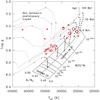 |
Fig. 1 Distribution of sample stars in the log g − Teff diagram. The 15 pulsators are represented by open circles. The size of a circle is a logarithmic measure of the fractional mass of the outer H-rich envelope in a given pulsator (the larger the circle, the more massive the hydrogen envelope). The small crosses give the locations of seven binary stars with masses derived from light curve modeling and spectroscopy. For comparison purposes, the solid (dotted) curves show a grid of zero age extended horizontal branches (ZAEHB’s) with zero (solar) metallicity defined by 3 values of the total mass and 8 values of the mass of the H envelope (from Fontaine et al. 2006). Typical evolutionary tracks for sdB stars (from Charpinet et al. 2002b) are also shown; the small dots indicate time steps of 107 yr from the initial ZAEHB position of a model at time t = 0. |
Given that binarity has no incidence on pulsational instabilities as pointed out above, there is no a priori reason to expect that the pulsator sample would lead to a biased mass distribution, unless our asteroseismological approach suffers from systematic effects. Along with the compelling result found by Charpinet et al. (2008) on PG 1336 − 018 as described in the Introduction, we obtain additional strong evidence that this is not the case by comparing the average masses of various subsamples: thus, the mean mass (straight average, not weighted) of the extended sample is 0.470 M⊙, that of the sample of 15 pulsators is 0.470 M⊙, that of the seven binary sdB components retained from Table 2 is 0.468 M⊙, that of the subsample of the 11 sdB components in binary systems is 0.471 M⊙, and that of the 11 apparently single stars is 0.468 M⊙.
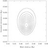 |
Fig. 2 Likelihood surface for our extended sample of 22 stars illustrated in the form of a contour plot. The maximum of the likelihood function is indicated by a small cross and is arbitrarily normalized to 1. It is characterized by a mean mass of μ = 0.4687 M⊙ and a standard deviation of σ = 0.0242 M⊙. The contours have values of 0.9 (smallest loop), 0.8, 0.7, 0.6, 0.5, 0.4, 0.3, 0.2, and 0.1 (largest loop). |
3. The mass distribution of sdB stars
We found it instructive at first to consider our extended sample of 22 stars and attempt to model it in terms of a normal distribution. In this, we follow part of the discussion presented by Kiziltan et al. (2010) on the mass distribution of neutron stars, a paper that we found particularly enlightening. Following these authors, we built a likelihood function for a normal mass distribution characterized by a mean value μ and a standard deviation σ, ![Mathematical equation: \begin{equation} L(\mu,\sigma) = {\prod^N_{i=1}~\left[2\pi \left(\sigma^2 + \sigma_i^2\right)\right]^{-1/2}~\exp {\left( {-\frac{(m_i - \mu)^2}{2(\sigma^2 + \sigma_i^2)}} \right)} }\cdot \end{equation}](/articles/aa/full_html/2012/03/aa18220-11/aa18220-11-eq82.png) (1)In this equation, the mi’s and σi’s are, respectively, the mass estimates and their associated uncertainties for each of the N = 22 stars retained from Tables 1 and 2. The uncertainties on the mass estimates are assumed to arise from normal distributions. Numerical maximization of the likelihood function in 2D space yields maximum likelihood estimates for the Gaussian mean μ and half-width σ of the normal mass distribution assumed for our sample of stars. Figure 2, showing the derived likelihood surface in the form of contours, summarizes the results of this optimization exercise. We find a mean mass of μ = 0.469 M⊙ and a standard deviation of σ = 0.024 M⊙1.
(1)In this equation, the mi’s and σi’s are, respectively, the mass estimates and their associated uncertainties for each of the N = 22 stars retained from Tables 1 and 2. The uncertainties on the mass estimates are assumed to arise from normal distributions. Numerical maximization of the likelihood function in 2D space yields maximum likelihood estimates for the Gaussian mean μ and half-width σ of the normal mass distribution assumed for our sample of stars. Figure 2, showing the derived likelihood surface in the form of contours, summarizes the results of this optimization exercise. We find a mean mass of μ = 0.469 M⊙ and a standard deviation of σ = 0.024 M⊙1.
We compare the measured masses of the sdB stars in our extended sample with the expectations of the derived normal distribution in Fig. 3. From top to bottom, and in order of appearence in Tables 1 and 2, we plotted the values of the inferred masses and their uncertainties for the 15 objects belonging to our asteroseismological sample (solid error bars), as well as those of the seven additional stars culled from the binary sample (dotted error bars). In comparison, the solid vertical line shows the mean value, while the two sets of dotted vertical lines define the central 68.3% (inner lines) and 95.4% (outer lines) probability intervals associated with the derived normal distribution.
Although Fig. 3 certainly suggests that the mass distribution of our sample of 22 stars can quite reasonably be modeled in terms of a Gaussian law, the “true” distribution does not have to be a normal one. We therefore decided to next construct a purely empirical, model-free mass distribution, but still based on the minimal assumption that the inferred σi’s associated with the measured masses obey normal distribution laws. Hence, an empirical mass distribution can readily be constructed by adding together suitably normalized Gaussians, each representing a measurement and its uncertainty.
Characteristics of the empirical mass distribution of sdB subdwarfs based on various samples.
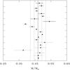 |
Fig. 3 Measured masses of sdB stars. The error bars indicate the ± 1σ uncertainties. The 15 stars culled from our asteroseismological sample are shown by solid error bars, while the seven objects taken from Table 2 are shown by dotted error bars. The solid vertical line illustrates the peak value of the likelihood function for our full sample of 22 stars, μ = 0.4687 M⊙, while the accompanying two sets of dotted vertical lines define the central 68.3% (inner lines) and 95.4% (outer lines) probability intervals associated with the assumed model normal distribution. |
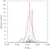 |
Fig. 4 Raw mass distribution of sdB stars (red curve) obtained by adding together 22 Gaussians, each representing a measurement defined by a mass value and its associated 1σ uncertainty. The individual Gaussians are shown in black; as solid curves for the 15 pulsators, and dotted curves for the seven objects culled from Table 2. The area under each individual Gaussian is normalized to the same value so as to correspond to the contribution of 1 star. The ordinate is on an arbitrary scale. The blue dotted curve shows the normal distribution characterized by μ = 0.4687 M⊙ and σ = 0.0242 M⊙. It is normalized in such a way as to have the same area under its curve as the raw distribution, corresponding to a total number of 22 objects. The dotted vertical line segments are used in the eventual conversion of the raw distribution (red curve) into the form of an histogram (see text). |
The outcome of this operation is shown in Fig. 4, where the red curve illustrates the resulting raw distribution. Clearly, there is no useful information, for example, in the two spikes that dominate the distribution, if not for the fact that they correspond simply to two stars with masses particularly accurately measured. Hence, it seems sensible to degrade the “resolution” of the raw distribution in order to get rid of this useless information. This is best done by binning the distribution in the form of an histogram. To help choosing the best binning strategy, we resorted to the normal distribution inferred above (the blue dotted curve in Fig. 4). From it, we picked a central mass bin centered on the mean value μ = 0.469 M⊙, and a bin width, or “resolution element”, equal to the standard deviation of σ = 0.024 M⊙. The resulting bin distribution is depicted by the vertical dotted line segments in Fig. 4.
The final outcome, and the central result of this paper, is the empirical mass distribution for sdB stars shown in the form of an histogram in Fig. 5. The distribution is sharply peaked around a mean value of 0.470 M⊙. Its median value is equal to 0.471 M⊙, essentially the same as the mean, which implies a rather symmetrical distribution. Some 15.85% of the stars in the distribution have masses smaller than 0.439 M⊙, and another 15.85% have masses larger than 0.501 M⊙.
We also obtained similar mass distributions for various subsamples of stars culled from Tables 1 and 2. Our results are summarized in Table 3. In particular, we find that the mass distribution derived from our sample of 15 pulsating sdB stars is practically indistinguishable from that of our extended sample. Indeed, it is characterized by a mean value of 0.470 M⊙, a median value of 0.470 M⊙, and a narrow range from 0.441 M⊙ to 0.499 M⊙ containing 68.3% of the stars in the sample. The shaded area in Fig. 5 illustrates that distribution of pulsators.
Otherwise, taking into account the small numbers of stars in the various subsamples, Table 3 suggests no detectable significant differences between the various distributions. Of particular interest, we find no important differences between the distributions derived from our sample of 15 pulsators (Table 1) and from the sample of seven sdB stars with masses obtained through classical methods (Table 2). Likewise, we find no significant differences between the mass distribution inferred from the 11 binary systems considered in this study and that based on the 11 apparently single stars.
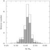 |
Fig. 5 Empirical mass distribution of sdB stars shown in the form of an histogram made of 14 equal-sized mass bins covering the range 0.2872 − 0.6260 M⊙. It is based on the raw distribution of our sample of 22 stars shown in Fig. 4. The dark area corresponds to our subsample of 15 pulsators. |
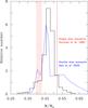 |
Fig. 6 Comparison of the empirical mass distribution of sdB stars based on our full sample of 22 stars (histogram) with the range of possible masses predicted by single star evolution according to Dorman et al. (1993); the red lines mark the (sharp) upper and (fuzzy) lower boundaries of this range. Another comparison is provided by the blue curve which shows one of the predicted mass distributions of sdB stars due to binary evolution according to Han et al. (2003). The blue curve has been normalized such that the area under it is equal to the area occuped by the histogram (corresponding to the total number of stars in the sample). |
4. Discussion
The empirical mass distribution for sdB stars that we presented above is certainly limited by the fact that the total number of stars involved is still rather small (15 in the asteroseismological sample, and 22 in the extended sample). Nevertheless, we found it interesting and instructive to compare it at the qualitative level with predictions of stellar evolution theory.
Figure 6 thus illustrates the empirical mass distribution (histogram) based on our extended sample in relation to the expected range of possible sdB masses (red boundaries) according to the calculations of Dorman et al. (1993) for single star evolution. The upper limit of the Dorman et al. range is rather sharply defined and corresponds, in their computations, to the limiting mass above which a star will ascend the AGB instead of becoming a sdB object. On the other hand, the lower limit is more fuzzy and corresponds to the still uncertain value of the required mass to ignite helium in the core for stars on the EHB.
Figure 6 further allows a comparison with one (blue curve) of the detailed mass distributions – as opposed to a simple mass range as in the previous case – predicted by Han et al. (2003) who investigated several binary star formation channels for sdB stars. Binary scenarios allow for the formation of broader wings in the mass distribution as compared to single star scenarios. The full mass distribution expected from such scenarios is given by the solid curve in Fig. 22 of Han et al. (2003). However, as discussed by these authors, care should be exercised when comparing that distribution with empirical data because it is sensitive to selection effects. In particular, in the present case, our sample stars all come from surveys that systematically discriminate against binary systems with main sequence companions that would be brighter than the sdB components. In that case, according to Han et al. (2003), we have to apply the so-called GK selection criterion to their theoretical mass distribution. This eliminates essentially all of the low-mass sdB stars produced by the Roche lobe overflow formation channel, and we are left with the dashed curve (the blue curve in our Fig. 6) in Fig. 22 of Han et al. (2003), made primarily of the products of common envelope evolution and stellar mergers.
We find that our empirical mass distribution agrees quite well with the expectations of stellar evolution theory, at least at the qualitative level. For instance, most of the stars (86%) in our extended sample have masses that fall right within the mass range (0.40 − 0.52 M⊙) predicted by Dorman et al. (1993) on the basis of single star evolution, while the presence of low- and high-mass wings in the distribution, expected from binary evolution scenarios, is also clearly revealed in our Figs. 5 and 6. There could be already an indication that the merger scenario produces too many (massive) stars as judged from the comparison of the predicted high-mass wing of the dotted curve with the rather symmetrical empirical distribution. Also, the average mass of the Han et al. (2003) distribution shown in Fig. 6 is 0.499 M⊙, to be compared with an average empirical mass of 0.470 M⊙. We warn, however, that this result is only suggestive at this stage. And indeed, it would be highly premature to attempt discriminating between single star and binary evolution scenarios on the basis of our empirical mass distribution as the numbers involved are still too small.
The encouraging results presented in this paper should provide added impetus toward the goal of building up an improved and more statistically significant empirical mass distribution for sdB stars in the years to come. In this endeavor, asteroseismology is likely to keep a central role, given that there are several additional targets (p-mode pulsators already observed from the ground, and g-mode pulsators being observed from space) that have already proven to be suitable for detailed seismic analyses.
A similar exercise, but this time for our sample of 15 pulsators, yields a mean mass of μ = 0.467 M⊙ and a standard deviation of σ = 0.027 M⊙.
Acknowledgments
This work was supported in part by the NSERC of Canada. G. Fontaine also acknowledges the contribution of the Canada Research Chair Program. S.C. and V.V.G. acknowledge financial support from “Programme National de Physique Stellaire” (PNPS) of CNRS/INSU, France.
References
- Allard, F., Wesemael, F., Fontaine, G., Bergeron, P., & Lamontagne, R. 1994, AJ, 107, 1565 [NASA ADS] [CrossRef] [Google Scholar]
- Billères, M., & Fontaine, G. 2005, in 14th European Workshop on White Dwarfs, ed. D. Koester, & S. Moehler (San Francisco: ASP), ASP Conf. Ser., 334, 635 [Google Scholar]
- Billères, M., Fontaine, G., Brassard, P., et al. 1997, ApJ, 487, L81 [NASA ADS] [CrossRef] [Google Scholar]
- Bloemen, S., Marsh, T. R., Østensen, R. H., et al. 2011, MNRAS, 410, 1787 [NASA ADS] [Google Scholar]
- Brassard, P., & Fontaine, G. 2008, in Hot Subdwarf Stars and Related Objects, ed. U. Heber, S. Jeffery, & R. Napiwotzki (San Francisco: ASP), ASP Conf. Ser., 392, 261 [Google Scholar]
- Brassard, P., Fontaine, G., Billères, M., et al. 2001, ApJ, 563, 1013 [CrossRef] [Google Scholar]
- Castellani, M., & Castellani, V. 1993, ApJ, 407, 649 [NASA ADS] [CrossRef] [Google Scholar]
- Charpinet, S., Fontaine, G., Brassard, P., et al. 1997, ApJ, 483, L123 [NASA ADS] [CrossRef] [PubMed] [Google Scholar]
- Charpinet, S., Fontaine, G., Brassard, P., & Dorman, B. 2002a, ApJS, 139, 487 [Google Scholar]
- Charpinet, S., Fontaine, G., Brassard, P., & Dorman, B. 2002b, ApJS, 140, 469 [NASA ADS] [CrossRef] [EDP Sciences] [Google Scholar]
- Charpinet, S., Fontaine, G., & Brassard, P. 2003, in White Dwarfs, ed. D. de Martino, R. Silvotti, J.-E. Solheim, & R. Kalytis (Dordrecht: Kluwer), NATO ASIB Proc., 105, 69 [Google Scholar]
- Charpinet, S., Fontaine, G., Brassard, P., et al. 2005a, in 14th European Workshop on White Dwarfs, ed. D. Koester, & S. Moehler (San Francisco: ASP), ASP Conf. Ser., 334, 619 [Google Scholar]
- Charpinet, S., Fontaine, G., Brassard, P., Green, E. M., & Chayer, P. 2005b, A&A, 437, 575 [NASA ADS] [CrossRef] [EDP Sciences] [Google Scholar]
- Charpinet, S., Fontaine, G., Brassard, P., et al. 2005c, A&A, 443, 251 [NASA ADS] [CrossRef] [EDP Sciences] [Google Scholar]
- Charpinet, S., Silvotti, R., Bonanno, A., et al. 2006a, A&A, 459, 565 [NASA ADS] [CrossRef] [EDP Sciences] [Google Scholar]
- Charpinet, S., Fontaine, G., Brassard, P., Chayer, P., & Green, E. M. 2006b, Mem. S.A.It., 77, 358 [NASA ADS] [Google Scholar]
- Charpinet, S., Van Grootel, V., Reese, D., et al. 2008, A&A, 489, 377 [NASA ADS] [CrossRef] [EDP Sciences] [Google Scholar]
- Charpinet, S., Brassard, P., Fontaine, G., et al. 2009, in Stellar Pulsations: Challenges for Theory and Observations (College Park: AIP), AIP Conf. Proc., 1170, 585 [Google Scholar]
- Charpinet, S., Van Grootel, V., Fontaine, G., et al. 2011, A&A, 530, A1 [NASA ADS] [CrossRef] [EDP Sciences] [Google Scholar]
- D’Cruz, N. L., Dorman, B., Rood, R. T., & O’Connell, R. W. 1996, ApJ, 466, 359 [NASA ADS] [CrossRef] [Google Scholar]
- Dorman, B., Rood, R. T., & O’Connell, R. W. 1993, ApJ, 419, 596 [CrossRef] [Google Scholar]
- Drechsel, H., Heber, U., Napiwotzki, R., et al. 2001, A&A, 379, 893 [NASA ADS] [CrossRef] [EDP Sciences] [Google Scholar]
- Fontaine, G., Brassard, P., Charpinet, S., et al. 2006, in Proc. SOHO18/GONG 2006/HELAS I Conf., Beyond the Spherical Sun, ESA SP-624, Sheffield, ed. K. Fletcher, & M. Thompson, published on CDROM, 32.1 [Google Scholar]
- For, B.-Q., Green, E. M., Fontaine, G., et al. 2010, ApJ, 708, 253 [NASA ADS] [CrossRef] [Google Scholar]
- Geier, S., Nesslinger, S., Heber, U., et al. 2007, A&A, 464, 299 [NASA ADS] [CrossRef] [EDP Sciences] [Google Scholar]
- Green, E. M., Liebert, J. W., & Saffer, R. A. 1997, in The Third Conference on Faint Blue Stars, ed. A. G. D. Philip, J. Liebert, R. Saffer & D. S. Hayes (Schenectady: L. Davis Press), 417 [Google Scholar]
- Green, E. M., Fontaine, G., Reed, M. D., et al. 2003, ApJ, 583, L31 [NASA ADS] [CrossRef] [Google Scholar]
- Han, Z., Podsiadlowski, P., Maxted, P. F. L., Marsh, T. R., & Ivanova, N. 2002, MNRAS, 336, 449 [NASA ADS] [CrossRef] [Google Scholar]
- Han, Z., Podsiadlowski, P., Maxted, P. F. L., & Marsh, T. R. 2003, MNRAS, 341, 669 [NASA ADS] [CrossRef] [Google Scholar]
- Heber, U. 1986, A&A, 155, 33 [NASA ADS] [Google Scholar]
- Heber, U. 1989, ARA&A, 47, 211 [Google Scholar]
- Heber, U., Drechsel, H., Carl, C., et al. 2005, in 14th European Workshop on White Dwarfs, ed. D. Koester, & S. Moehler (San Francisco: ASP), ASP Conf. Ser. 334, 357 [Google Scholar]
- Kilkeny, D., Koen, C., O’Donoghue, D., & Stobie, R. S. 1997, MNRAS, 285, 640 [Google Scholar]
- Kiziltan, B., Kottas, A., & Thorsett, S. E. 2010, ApJ, submitted [arXiv:1011.4291] [Google Scholar]
- Klepp, S., & Rauch, T. 2011, A&A, 531, L7 [NASA ADS] [CrossRef] [EDP Sciences] [Google Scholar]
- Lee, J. W., Kim, S., Kim, C., et al. 2009, AJ, 137, 3181 [NASA ADS] [CrossRef] [Google Scholar]
- Lisker, T., Heber, U., Napiwotzki, R., et al. 2005, A&A, 430, 223 [NASA ADS] [CrossRef] [EDP Sciences] [Google Scholar]
- Maxted, P. F. L., Heber, U., Marsh, T. R., & North, R. C. 2001, MNRAS, 326, 1391 [NASA ADS] [CrossRef] [Google Scholar]
- Mengel, J. G., Norris, J., & Gross, P. G. 1976, ApJ, 204, 488 [NASA ADS] [CrossRef] [Google Scholar]
- Orosz, J. A., & Wade, R. A. 1999, MNRAS, 310, 773 [NASA ADS] [CrossRef] [Google Scholar]
- Østensen, R. W., Green, E. M., Bloemen, S., et al. 2010, MNRAS, 408, 51 [Google Scholar]
- Randall, S. K., Green, E. M., Fontaine, G., et al. 2006a, ApJ, 645, 1464 [NASA ADS] [CrossRef] [Google Scholar]
- Randall, S. K., Fontaine, G., Charpinet, S., et al. 2006b, ApJ, 648, 637 [NASA ADS] [CrossRef] [Google Scholar]
- Randall, S. K., Green, E. M., Van Grootel, V., et al. 2007, A&A, 476, 1317 [NASA ADS] [CrossRef] [EDP Sciences] [Google Scholar]
- Randall, S. K., Van Grootel, V., Fontaine, G., Charpinet, S., & Brassard, P. 2009, A&A, 507, 911 [NASA ADS] [CrossRef] [EDP Sciences] [Google Scholar]
- Saffer, R. A., Bergeron, P., Koester, D., & Liebert, J. 1994, ApJ, 432, 351 [NASA ADS] [CrossRef] [Google Scholar]
- Van Grootel, V. 2008, Ph.D. Thesis, Université de Toulouse and Université de Montréal [Google Scholar]
- Van Grootel, V., Charpinet, S., Fontaine, G., & Brassard, P. 2008a, A&A, 483, 875 [NASA ADS] [CrossRef] [EDP Sciences] [Google Scholar]
- Van Grootel, V., Charpinet, S., Fontaine, G., et al. 2008b, A&A, 488, 685 [NASA ADS] [CrossRef] [EDP Sciences] [Google Scholar]
- Van Grootel, V., Charpinet, S., Fontaine, G., & Brassard, P. 2010a, Ap&SS, 329, 217 [NASA ADS] [CrossRef] [Google Scholar]
- Van Grootel, V., Charpinet, S., Fontaine, G., et al. 2010b, ApJ, 718, L97 [NASA ADS] [CrossRef] [EDP Sciences] [Google Scholar]
- Van Grootel, V., Charpinet, S., Fontaine, G., Green, E. M., & Brassard, P. 2010c, A&A, 524, 63 [Google Scholar]
- van Spaandonk, L., Fontaine, G., Brassard, P., & Aerts, C. 2008, Commun. Asteroseismol., 156, 35 [NASA ADS] [CrossRef] [Google Scholar]
- Vuckovic, M., Aerts, C., Østensen, R. H., et al. 2007, A&A, 471, 605 [NASA ADS] [CrossRef] [EDP Sciences] [Google Scholar]
- Wils, P., di Scala, G., & Otero, S. A. 2007, IBVS, 5800, 1 [NASA ADS] [Google Scholar]
- Wood, J. H., & Saffer, R. A. 1999, MNRAS, 305, 820 [NASA ADS] [CrossRef] [Google Scholar]
All Tables
Hot B subdwarf stars with masses determined by light curve modeling and spectroscopy in binary systems.
Characteristics of the empirical mass distribution of sdB subdwarfs based on various samples.
All Figures
|
Fig. 1 Distribution of sample stars in the log g − Teff diagram. The 15 pulsators are represented by open circles. The size of a circle is a logarithmic measure of the fractional mass of the outer H-rich envelope in a given pulsator (the larger the circle, the more massive the hydrogen envelope). The small crosses give the locations of seven binary stars with masses derived from light curve modeling and spectroscopy. For comparison purposes, the solid (dotted) curves show a grid of zero age extended horizontal branches (ZAEHB’s) with zero (solar) metallicity defined by 3 values of the total mass and 8 values of the mass of the H envelope (from Fontaine et al. 2006). Typical evolutionary tracks for sdB stars (from Charpinet et al. 2002b) are also shown; the small dots indicate time steps of 107 yr from the initial ZAEHB position of a model at time t = 0. |
| In the text | |
|
Fig. 2 Likelihood surface for our extended sample of 22 stars illustrated in the form of a contour plot. The maximum of the likelihood function is indicated by a small cross and is arbitrarily normalized to 1. It is characterized by a mean mass of μ = 0.4687 M⊙ and a standard deviation of σ = 0.0242 M⊙. The contours have values of 0.9 (smallest loop), 0.8, 0.7, 0.6, 0.5, 0.4, 0.3, 0.2, and 0.1 (largest loop). |
| In the text | |
|
Fig. 3 Measured masses of sdB stars. The error bars indicate the ± 1σ uncertainties. The 15 stars culled from our asteroseismological sample are shown by solid error bars, while the seven objects taken from Table 2 are shown by dotted error bars. The solid vertical line illustrates the peak value of the likelihood function for our full sample of 22 stars, μ = 0.4687 M⊙, while the accompanying two sets of dotted vertical lines define the central 68.3% (inner lines) and 95.4% (outer lines) probability intervals associated with the assumed model normal distribution. |
| In the text | |
|
Fig. 4 Raw mass distribution of sdB stars (red curve) obtained by adding together 22 Gaussians, each representing a measurement defined by a mass value and its associated 1σ uncertainty. The individual Gaussians are shown in black; as solid curves for the 15 pulsators, and dotted curves for the seven objects culled from Table 2. The area under each individual Gaussian is normalized to the same value so as to correspond to the contribution of 1 star. The ordinate is on an arbitrary scale. The blue dotted curve shows the normal distribution characterized by μ = 0.4687 M⊙ and σ = 0.0242 M⊙. It is normalized in such a way as to have the same area under its curve as the raw distribution, corresponding to a total number of 22 objects. The dotted vertical line segments are used in the eventual conversion of the raw distribution (red curve) into the form of an histogram (see text). |
| In the text | |
|
Fig. 5 Empirical mass distribution of sdB stars shown in the form of an histogram made of 14 equal-sized mass bins covering the range 0.2872 − 0.6260 M⊙. It is based on the raw distribution of our sample of 22 stars shown in Fig. 4. The dark area corresponds to our subsample of 15 pulsators. |
| In the text | |
|
Fig. 6 Comparison of the empirical mass distribution of sdB stars based on our full sample of 22 stars (histogram) with the range of possible masses predicted by single star evolution according to Dorman et al. (1993); the red lines mark the (sharp) upper and (fuzzy) lower boundaries of this range. Another comparison is provided by the blue curve which shows one of the predicted mass distributions of sdB stars due to binary evolution according to Han et al. (2003). The blue curve has been normalized such that the area under it is equal to the area occuped by the histogram (corresponding to the total number of stars in the sample). |
| In the text | |
Current usage metrics show cumulative count of Article Views (full-text article views including HTML views, PDF and ePub downloads, according to the available data) and Abstracts Views on Vision4Press platform.
Data correspond to usage on the plateform after 2015. The current usage metrics is available 48-96 hours after online publication and is updated daily on week days.
Initial download of the metrics may take a while.