| Issue |
A&A
Volume 539, March 2012
|
|
|---|---|---|
| Article Number | A105 | |
| Number of page(s) | 13 | |
| Section | Cosmology (including clusters of galaxies) | |
| DOI | https://doi.org/10.1051/0004-6361/201118162 | |
| Published online | 01 March 2012 | |
Deep Chandra observation of the galaxy cluster WARPJ1415.1+3612 at z =1
An evolved cool-core cluster at high redshift
1
European Space Astronomy Centre (ESAC)/ESA,
Madrid,
Spain
e-mail: This email address is being protected from spambots. You need JavaScript enabled to view it.
2
INAF, Osservatorio Astronomico di Trieste, via G.B. Tiepolo
11, 34131
Trieste,
Italy
3
INFN, Istituto Nazionale di Fisica Nucleare,
Trieste,
Italy
4
European Southern Observatory, Karl-Schwarzchild Strasse 2, 85748
Garching,
Germany
5
Dipartimento di Astronomia, via Ranzani 1, 40127
Bologna,
Italy
6
Istituto di Radioastronomia - INAF, via P. Gobetti
101, 40129
Bologna,
Italy
Received: 27 September 2011
Accepted: 15 January 2012
Abstract
Aims. Using the deepest (370 ks) Chandra observation of a high-redshift galaxy cluster, we perform a detailed characterization of the intra-cluster medium (ICM) of WARPJ1415.1+3612 at z = 1.03, particularly its core region. We also explore the connection between the ICM core properties and the radio/optical properties of the brightest cluster galaxy (BCG).
Methods. We perform a spatially resolved analysis of the ICM to obtain temperature, metallicity and surface brightness profiles over the 8–400 kpc radial range. We measure the following cool-core diagnostics: central temperature drop, central metallicity excess, central cooling time, and central entropy. Using the deprojected temperature and density profiles, we accurately derive the cluster hydrostatic mass at different overdensities. In addition to the X-ray data, we use archival radio VLA imaging and optical GMOS spectroscopy of the central galaxy to investigate the feedback between the central galaxy and the ICM.
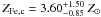
Results. Our spatially resolved spectral analysis shows a significant temperature drop from a maximum of 8.0 keV to a projected core value Tc = 4.6 ± 0.4 keV, and a remarkably high central iron abundance peak, ZFe,c = 3.60-0.85+1.50 Z⊙, measured within a radius of 12 kpc. We measure M500 = M(r < R500) = 2.4 ± 0.4 M⊙ and a corresponding gas fraction fgas = 0.10 ± 0.02. The central cooling time is shorter than 0.1 Gyr and the entropy Kc is equal to 9.9 keV cm2. We detect a strong [OII] emission line in the optical spectra of the BCG with an equivalent width of –25 Å, for which we derive a star formation rate within the range 2–8 M⊙ yr-1. The VLA data reveals a central radio source coincident with the BCG with a luminosity L1.4 GHz = 2.0 × 1025 W Hz-1, and a faint one-sided jet-like feature with an extent of ~80 kpc. We do not find clear evidence for cavities associated to the radio AGN activity.
Conclusions. Our analysis shows that WARPJ1415 has a well developed cool-core with ICM properties similar to those found in the local Universe. Its properties and the clear sign of feedback activity found in the central galaxy in the optical and radio bands, show that feedback processes are already established at z ~ 1 (a lookback time of 7.8 Gyr). In addition, the presence of a strong metallicity peak shows that the central regions have been promptly enriched by star formation processes in the central galaxy already at z > 1. Our results significantly constrain the timescale for the formation and self-stabilization of cool-cores.
Key words: galaxies: clusters: intracluster medium / X-rays: galaxies: clusters / galaxies: high-redshift / galaxies: clusters: individual: WARPJ1415.1+3612
© ESO, 2012
1. Introduction
Galaxy clusters are dynamical environments hosting complex astrophysical phenomena, that provide us with a wealth of information on the intricate processes that shape the cosmic large-scale structure and galaxy evolution (see reviews by Fabian 1994; Rosati et al. 2002; Voit 2005).
The intracluster medium (ICM) is the dominant baryonic component of galaxy clusters, a hot plasma emitting X-ray radiation via thermal bremsstrahlung. High-resolution X-ray observations show that the surface brightness of the ICM of about half of the local clusters is peaked in their central regions, where the inferred cooling time of the gas is shorter than the typical dynamical time (see Fabian 1994, for a review on cooling flows; and Hudson et al. 2010, for more recent results). However, X-ray spectroscopy always shows a gas temperature floor, indicating that some distributed source of heating must stop the cooling process (see Peterson & Fabian 2006, and references therein). In the current framework, the dominant heating source that prevents the overcooling of the ICM is likely to be an AGN fueling a massive central black hole, leading to an outburst which can heat the ICM via shocks, buoyantly rising bubbles inflated by radio lobes, or dissipation of sound waves (see McNamara & Nulsen 2007, for a review).
The so-called cool-core phenomenon is observed in different wavebands depending on the cluster component under investigation. Among them: the ICM (X-ray), the brightest cluster galaxy (BCG, optical), cold molecular gas (IR), and the central AGN (radio). The onset of star formation activity in the central galaxy (otherwise a passive, early-type galaxy) is a well-known manifestation of this phenomenon (Crawford et al. 1999; McNamara et al. 2007; Donahue et al. 2010). However, nuclear activity in the central cluster galaxy is expected to play the major role in regulating the cool-core thermodynamics, as suggested by the observed interactions between the radio jets and the ICM and the scaling relations among total radio power and ICM properties observed in the X-ray band (Birzan et al. 2008). These processes are shown in the spectacular combined images of nearby clusters in the radio and X-ray bands, where cavities and ripples in the ICM are observed to correspond to non-thermal radio emission (Blanton et al. 2001; Birzan et al. 2004; Wise et al. 2007; Sanders & Fabian 2007; Sanders et al. 2009, and many others).
There is increasing evidence from radio and X-ray observations of local clusters that the formation of bubbles due to radio jets associated to the central AGN may effectively satisfy the energy balance between cooling and heating in cool-core regions (Blanton 2001; Ehlert et al. 2011). In this respect, the radio luminosity of the central galaxy provides an important link between the black hole activity and the state of the intracluster medium.
To date, systematic studies of the cool-core phenomenon including X-ray, optical and radio data to understand how the feedback mechanism shapes the evolution of cool-cores have been limited to samples of nearby clusters (e.g., Heckman et al. 1989; Birzan et al. 2004; Cavagnolo et al. 2008; O’Dea et al. 2008; Mittal et al. 2009; Sun 2009; McDonald et al. 2010), reaching a redshift up to ⟨ z ⟩ = 0.3 (Samuele et al. 2011). These studies show clear correlations involving the radio luminosity of the central AGN, optical emission lines (e.g. Hα), excess IR/UV emission, and the core entropy of the ICM.
The extension of these studies to high-redshift can provide important clues also on the timescales of the metal enrichment mechanisms of the ICM, a process that encompasses different phases of the cool-core phenomenon. Iron, the main metal locked in the ICM, is produced primarily by type Ia supernovae, while iron and other heavy elements produced by both type Ia and type II SNe hosted by the cluster early-type galaxies (Renzini et al. 1993) are eventually diffused into the ICM via galactic winds and ram pressure striping. According to local studies, the excess iron mass found in cool-cores is directly linked to the brightest cluster galaxies (Böhringer et al. 2004; De Grandi et al. 2004). A complete understanding of the formation and evolution of cool-cores should encompass all these aspects.
Recent results indicate a moderate evolution in the bulk of the cool-core cluster population out to z = 1.3, with an apparent lack of very strong cool-core clusters at high redshifts (Santos et al. 2008, 2010). However, to adequately compare the characteristics of distant and nearby cool-core clusters, we require deep, high-resolution X-ray data of distant clusters. The study of cool-cores at high-redshift will not only place an upper limit on the formation timescale of cool-cores, but will also reveal the strength of the interactions between the diffuse baryons and the brightest central galaxy (BCG) at an epoch when the most massive clusters are still assembling.
In this paper we provide a detailed investigation of the ICM of the X-ray selected cluster WARPJ1415.1+3612 (hereafter WARPJ1415) at z = 1.03 (Perlman et al. 2002), using a recently acquired deep Chandra observation. This cluster was chosen as the strongest high-z cool-core cluster based on the analysis of its surface brightness properties (Santos et al. 2010). Using a multi-wavelength dataset comprising radio VLA data, archival optical GEMINI-GMOS spectroscopy and imaging from HST/ACS F775W, and SUBARU-Suprime (BVRiz) we study the central galaxy and its interactions with the hot plasma. The analysis presented here is the first detailed study of the feedback process in a cool-core at such high-redshift.
The paper is organized as follows: in Sect. 2 we describe the X-ray data reduction procedures, including the detailed spatially resolved spectroscopic analysis of the ICM. In Sect. 3 we obtain the temperature and metallicity profiles. We perform the deprojection analysis and present the mass profile in Sect. 4. We investigate the surface brightness properties of the ICM in Sect. 5 and we accurately measure several cool-core diagnostics, namely cSB, the central cooling time and central entropy. In Sect. 6 we present the radio and optical properties of the BCG and explore the connection between the BCG and the ICM core properties. Our conclusions are summarized in Sect. 7.
The cosmological parameters used throughout the paper are: H0 = 70 km s-1 Mpc-1, ΩΛ = 0.7 and Ωm = 0.3. Quoted errors are at the 1-σ level, unless otherwise stated.
2. X-ray data reduction and spectral analysis
2.1. The X-ray dataset
The galaxy cluster WARPJ1415 was detected in the Wide Angle ROSAT Pointed Survey (Jones et al. 1998; Perlman et al. 2002). This survey provided several high-redshift galaxy clusters based on serendipitous detections of extended sources in targeted ROSAT PSPC observations. The survey covers an area of 71 deg2 and contains a complete sample of 129 X-ray selected clusters down to a flux limit of S ~ 6.5 × 10⁻¹⁴ erg s-1 cm2.
A deep, 280 ks ACIS-S observation of WARPJ1415 was awarded to our group in Chandra AO 12 (PI J. Santos). An additional 90 ks observation with ACIS-I (taken in 2004, PI H. Ebeling) was used in our analysis. The Chandra exposure time sums up to a total 370 ks (obsid 4163, 12255, 12256, 13118, 13119). This dataset represents the deepest Chandra observation of a cluster at z ≃ 1, enabling the most detailed X-ray analysis of any such high redshift galaxy cluster. Previous studies of distant X-ray clusters with comparable depth used both shallow Chandra and XMM-Newton data (see Maughan et al. 2008), and therefore do not reach the angular resolution to study the inner regions of the ICM distribution. In the case of WARP1415, angular resolution has a paramount relevance, since it allows us to resolve the density, temperature and metal distribution within the cool-core region on a scale as small as ~10 kpc, and hence to shed light on the complex physics of the cool-core region at a look back time of 8 Gyr.
We also examined the XMM-Newton archival data on WARPJ1415. We find that after removing the time intervals of high-background, the useful exposure time is about 17 ks for MOS and 14 ks for PN. Given the modest exposure time and the much lower angular resolution of XMM-Newton, we do not include this dataset in our analysis.
2.2. Data reduction
We performed a standard data reduction starting from the level = 1 event files, using the CIAO 4.3 software package, with the most recent version of the Chandra Calibration Database at the time of writing (CALDB 4.4.5). We ran the acis_process_events task to update the data calibration, including the tgain correction1. Since both ACIS-I and ACIS-S observations were taken in the VFAINT mode, we set the check_vf_pha key to yes to flag background events that are most likely associated with cosmic rays and distinguish them from real X-ray events. With this procedure, the ACIS particle background can be significantly reduced compared to the standard grade selection. We also applied the CTI correction to the ACIS-I observation (taken with the temperature of the Focal Plane equal to 153 K). This procedure allows us to recover the original spectral resolution partially lost because of the CTI (see Grant et al. 2004). The correction applies only to ACIS-I data, since the ACIS-S3 did not suffer from radiation damage. The data were filtered to include only the standard event grades 0, 2, 3, 4 and 6. We did not remove the acis_detect_afterglow correction since all our data have a SDP version larger than 7.4.02. Nevertheless, we checked visually for hot columns left after the standard reduction, finding none. We also identified the flickering pixels as the pixels with more than two events contiguous in time, where a single time interval was set to 3.3 s. For exposures taken in VFAINT mode, there are no flickering pixels left after filtering out bad events. We filtered time intervals with high background by performing a 3σ clipping of the background level in the 0.5−7 keV band by using the script analyze_ltcrv. We did not detect any high background interval in both ACIS-I and ACIS-S data (nominally the removed exposure time is less than 0.5% for ACIS-I and less than 0.2% for ACIS-S). We remark that our spectral analysis is not affected by any possible residual flare unnoticed in the 0.5–7 keV band, since we compute the background from source-free regions around the cluster, thus taking into account any possible spectral distortion of the background itself. Finally, all the ACIS-S obsid were merged together with the merge_all tool. ACIS-S and ACIS-I are kept separated both for imaging and for spectral analysis, as described in the following sections.
2.3. Spectral analysis
We produced soft (0.5–2 keV) and hard (2–7 keV) band images with the full Chandra resolution (1 pixel = 0.492 arcsec). We computed the cluster center in the soft-band by measuring the position at which the signal-to-noise ratio (S/N) within circles of different radii is maximum. Following this procedure we assign the X-ray center of the cluster to RA = 14:15:11.08, Dec = +36:12:03.1. This position also corresponds to the peak of the surface brightness emission. We remark that we did not detect any point source which could significantly contribute to the core emission, by carefully inspecting the 0.5–2.0 keV and the 2.0–7.0 keV X-ray images.
The spectral analysis is performed as follows: starting from the cluster center, we draw rings at different radii and compute the S/N in the total 0.5–7 keV band for the ACIS-S image, which has a signal much stronger than the ACIS-I image. In order to achieve a good compromise between the S/N ratio in each ring and the total number of rings, we set a minimum S/N ≥ 24 within 25″, decreasing at larger radii down to 14 in the outermost radius. This ensures that we have always more than 650 net counts in the 0.5–7 keV band in each ring (with the exception of the central bin with 500 net counts), for a total of nine rings. We adopted the same set of circular rings in the ACIS-I image, despite the net counts in each ring are typically less then 100. In the last radial bin (300–400 kpc), we used only ACIS-S, since there is no useful signal in the ACIS-I data.
We extracted spectra for each ring from the ACIS-S and ACIS-I data separately. The response matrices and the ancillary response matrices were computed for each obsid respectively with mkacisrmf and mkwarf, for the same regions where the spectra were extracted. A single arf and rmf files for each ACIS-S spectrum were finally obtained by summing over the 4 ACIS-S obsid with addarf and addrmf, respectively. We detected 7500 (6200 in ACIS-S and 1300 in ACIS-I) photons within 50″, corresponding to 400 kpc.
We selected the background from empty regions of the same CCD in which the cluster is located. This is possible since the signal from the cluster has a total extension of less than 1 arcmin, as opposed to the 8′ size of the ACIS-I/-S chips. The background region is scaled to the source files by the ratio of their geometrical areas. In principle, the background regions may partially overlap with the outer virialized regions of the clusters. However, the cluster emission from these regions is negligible with respect to the instrumental background, and does not affect our results. Our background subtraction procedure, on the other hand, has the advantage of providing the best estimate of the background for that specific observation.
The background is extracted (both for ACIS-I and ACIS-S data) from 3 circular regions nearby the clusters, up to a maximum distance of 3 arcmin, and with a minimum distance of 1.2 arcmin. The size of each background region varies between 50 to 70 arcsec in radius, in order to ensure the background is sampled from a region larger by at least a factor of 10 with respect to the outermost ring. We repeated the measurement with other background regions selected with these criteria and found no significant differences in the final results.
The background spectra were scaled by the geometrical factor between the background and source regions before subtraction. Our spectral analysis is expected to be robust against background variations and vignetting effects thanks to the high S/N set for our circular rings (S/N of 25 except in the two outermost rings, where we have S/N = 20 and 15) and to the sparse sampling of the background. To show this, we also compute the scaling factors using the ratio of the exposure maps of the source and background regions, and repeat the spectral analysis. In all cases we obtain results in excellent agreement with those obtained with the simple geometrical scaling. We remark that a full treatment of the vignetting effects would imply modeling the background by treating each component separately. We do not apply this procedure in our paper since it would not introduce any noticeable improvement in the final results.
The spectra of each ring were analyzed with XSPEC v12.6 (Arnaud et al. 1996) and fitted with a single-temperature mekal model (Kaastra 1992; Liedahl et al. 1995) using the solar abundance of Asplund et al. (2005)3. The fits were performed over the energy range 0.5−8.0 keV. The free parameters in our spectral fits are temperature, metallicity and normalization. The local absorption is fixed to the Galactic neutral hydrogen column density (NH) measured at the cluster position (Wilms et al. 2000) and equal to NH = 1.05 × 1020 cm-2, and the redshift is fixed to z = 1.03. We used Cash statistics applied to the source plus background, which is preferable for low S/N spectra (Nousek & Shue 1989).
The spectra were binned only to one photon per energy bin. The use of Cash statistics with background subtracted spectra has been used in previous works, and validated with spectral simulations in the case of typical AGN (see Fig. 2 in Tozzi et al. 2006). The same results were obtained for thermal spectra typical of clusters.
The global temperature and abundance values were measured in the region of maximum S/N in the ACIS-S data, which corresponds to a radius Rext = 32″ centered around the cluster position. The spectrum extracted from this region allows us to measure temperature and Fe abundance with unprecedented accuracy at such an high redshift. The best fit values are  keV and
  . In addition, the strong Kα Fe line allow us to measure the redshift with an accuracy of less than 1%:
  (see Fig. 1). The same analysis performed with the ACIS-I data provides consistent results with larger uncertainties. These global values are still consistent with the values measured with a previous CALDB version by Balestra et al. (2007), using the 90 ks ACIS-I data. Our temperature measurement is in agreement, albeit with significantly improved accuracy, with those found by Maughan et al. (2006) in their analysis of the XMM-Newton data, and by Maughan et al. (2008) in their analysis of the ACIS-I Chandra data. However, we note that previous measurements of the Fe abundance with Chandra gave very low values, at variance with our findings.
We will not use the average values of temperature and metal abundance obtained from the highest S/N region in the rest of this study.
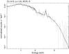 |
Fig. 1 Folded global spectrum of WARPJ1415 extracted from a circular region with radius of 32″ in the ACIS-S data (crosses) fitted with a mekal model (continuous line). The redshifted Kα line complex of hydrogen-like and helium-like iron (Fe XXV, XXVI) is clearly visible at ~3.5 keV. |
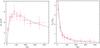 |
Fig. 2 Left panel: observed projected temperature profile of WARP1415 (red points) and the corresponding fit (red dashed line) compared to the deprojected measured temperature values (blue solid line). Right panel: same as left panel for the iron abundance profile. The 68% uncertainty in the fitted curves is very close to the typical error bars of the measured projected quantities at similar radii, and it is not shown for the sake of clarity. |
3. Projected temperature and metallicity profiles
Nearby cool-core clusters are characterized by several particular features in the central ICM, most of which require spatially resolved X-ray data and are therefore challenging to measure in the typical low S/N observations of high-redshift clusters. In the following subsections, we discuss in detail the spatially resolved properties of the ICM in WARPJ1415.
3.1. Projected temperature profile and map
The most distinctive sign of a cool-core is a temperature drop towards the cluster center, usually down to a third/half of the global cluster temperature (see, e.g., Peterson et al. 2003). A resolved temperature drop at high-redshift has only been observed in 3C 186 at z = 1.1 (Siemiginowska et al. 2010), a cluster that harbors a bright quasar in its center. More recently, the analysis of relatively shallow Chandra data of SPT-CL J2106-5844, a galaxy cluster at z = 1.1 discovered with the South Pole Telescope, hints at a temperature drop from  keV to
  keV in the core (Foley et al. 2011), with a drop factor of 1.7 ± 0.5. Similarly, the very massive merging cluster ACT-CL J0102-4215 at z = 0.87, shows temperature variations ranging from 22 ± 6 to 6.6 ± 0.7 keV (Menanteau et al. 2011), corresponding to a drop factor of ~2, from the global, core-excluded temperature, to the cluster center.
To measure the projected temperature profile of CL1415 we fitted the spectra of the rings obtained with the procedure described in Sect. 2. For each ring we combined the ACIS-S and ACIS-I data. Despite the fact that the majority of the signal is provided by the ACIS-S data, the use of the ACIS-I spectra allows us to obtain slightly smaller error bars with respect to the analysis based on the ACIS-S data only. In addition, the ACIS-S analysis shows no significant difference with respect to the combined analysis. Therefore, from now on we refer to the combined (ACIS-I+ACIS-S) spectral analysis.
The projected temperature profile is shown in Fig. 2, left panel. We are able to trace the temperature profile out to 400 kpc with an accuracy of the order of 10%, reaching 20% in the outermost bin (1-σ error). The innermost bin has a size of ~20 kpc, while the outermost bin has a size of ~100 kpc. We measure a significant central temperature drop with Tc = 4.6 ± 0.4 at R < 20 kpc, which is nearly half of the maximum cluster temperature, kT = 8.0 ± 1.2 keV, reached at r = 80 kpc. The ICM temperature drop, from the maximum value to the core value, is measured to be 1.7 ± 0.3. Clearly, the observed drop depends also on the capability of measuring the temperature in the very center of the cool core, which in turn depends on the angular resolution and on the S/N. Therefore, it is dangerous to use solely the measured temperature drop as an indication of the cool core strength.
To further investigate the temperature structure of WARP1415, we produced a temperature map. We map a square region of 40′′ by side centered on the cluster, extracting circular regions spaced by 2′′. Each circular region has a radius ranging from 3′′ to 10′′ going from the cluster center to the outer regions. Clearly, the spectra assigned to each pixel are not independent to each other, so the temperature map is actually a smoothed map, with a smoothing length increasing with the distance form the cluster center. The temperature map of WARP1415 is shown in Fig. 3, where we masked out the pixels where the 1 sigma error on the temperature is larger than 50%. In addition to the cool-core, which appears smooth and round within a radius of 3′′ (the minimum smoothing length of the map) we notice some anisotropy in the temperature profile, with a difference of about –2 keV in one sector at a distance of about 80 kpc (the distance where the temperature is maximum). We will discuss further this feature in Sect. 6.
3.2. Projected iron abundance profile
A prominent peak in the iron distribution is always associated with the ICM of local cool-core clusters. The origin of this iron excess with respect to the almost constant value measured in the outer regions is ascribed mostly to Type Ia supernovae (e.g. De Grandi et al. 2004). There is no consensus yet in the literature on the origin of the iron peak and timescale of its buildup. While some studies of local cool-cores favor long enrichment times (>5 Gyr), and describe the metal excess as a long lived phenomenon (Böhringer et al. 2004), the lack of high-z data has prevented a more accurate assessment of this important aspect.
In this section, we trace the spatial distribution of iron in the cluster ICM out to r = 400 kpc, as obtained by the spatially resolved, combined spectral analysis. In Fig. 2, we present the ICM iron abundance profile in solar units, where the solar abundance is set to the value of Asplund et al. (2005). We detect an unusually high central Fe value in the ICM of WARPJ1415, 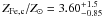 . Even taking into account the associated large error bar, such a high abundance level has only been reported in the local cluster Centaurus (Graham et al. 2006). The implication of this high iron concentration and the associated iron mass are discussed in Sect. 6.5. We investigated also the iron abundance map obtained along with the temperature map, but we do not find any significant anisotropy in the iron abundance distribution.
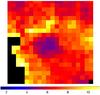 |
Fig. 3 Temperature map obtained in a square region 40″ × 40″ centered on the cluster. The colorbar indicates the temperature scale in keV. Pixels where the 1 sigma error is larger than 50% are masked in black. See text for details. |
3.3. Other metals
In addition to iron, alpha elements (Si, Ni, S, Mg) produced by core-collapse supernovae (SNII) contribute significantly to the enrichment of the ICM (e.g. De Grandi & Molendi 2009). A spatially resolved analysis of metals other than iron is not feasible. Nevertheless, we searched for emission line of other elements in the spectrum extracted from the inner 32′′. Metal lines were visually explored changing manually the abundance of each element. A given element was then removed whenever its presence was irrelevant to the best fit spectrum. Therefore, all metals were initially unconstrained, and progressively we froze to 0.3 the metals which do not contribute significantly to the folded spectrum. This procedure can be used to identify possible low S/N emission lines, by setting the corresponding element to zero the C-statistics increases by ΔC > 3. With this method, we confirmed the detection of the elements Si, S and Ni at 2 σ level. The nominal best fit values are: ZSi = 1.9 ± 0.7 Z⊙; ZS = 1.3 ± 0.7 Z⊙ and ZNi = 3.6 ± 1.7 Z⊙. This is the first detection of these elements in the spectrum of a cluster at z ≃ 1, but the lack of spectral resolution and S/N prevent us from computing a meaningful α/Fe profile and to derive robust constraints on the enrichment sources of the ICM.
4. Deprojection and mass profile
The next step in our analysis is to compute the deprojected temperature and metal abundance profiles, and then to compute total and gas masses. The direct deprojection of the observed profile with the projct model within XSPEC is not feasible due to the errors on the temperature and the coarse binning. For the best exploitation of our data we proceeded as follows. First we fitted the projected temperature and iron abundance profiles. For the temperature we use the functional form of Vikhlinin et al. (2006):  (1)where we set b = c/0.45 (as suggested in Maughan et al. 2007) and therefore we are left with 7 free parameters.
This functional form is usually taken to represent the 3D temperature distribution, and projected to be fit to the observed projected temperature profile. Instead, we treat r in Eq. (1) as a projected radius and fit the model to the projected temperature profile directly. The best fitting model is then deprojected to obtain the 3D temperature profile.
As for the iron abundance, we adopt a double beta model (Cavaliere & Fusco-Feminano 1976):  (2)which has 6 free parameters. Therefore we can estimate the projected temperature and Fe abundance of WARPJ1415 at any given radius using Eqs. (1) and (2) with the best-fit parameters plugged in. The next step is to deproject directly the analytical renditions of the temperature and abundance profile at the same time. Clearly, when deprojecting the best fit temperature and metallicity profiles, we want to preserve the full information coming from the surface brightness in order to directly obtain also the electron volume density ne as a function of the radius. We adopt a finer binning of the surface brightness profile, with the requirement of keeping the error on the normalization of each spectrum at the level of 5–10%. This is obtained by selecting rings with a minimum S/N of 15. We used 20 rings with a width ranging from 2′′ to 15′′ for increasing radii. We assigned a temperature and iron abundance to each ring according to Eqs. (1) and (2), respectively, computed at the central radius of each ring. We normalized each spectrum in order to have the same predicted net count rate as observed in the real image in the 0.5–2 keV band. We then simulated a spectrum for each ring with a very high S/N. The deprojection was obtained with projct, so that we include at the same time the effects of temperature and Fe abundance. In Fig. 2, we show the projected data with the best-fit model (dashed line) and the corresponding deprojected profile (solid line).
The best fit normalization of the deprojected spectra is linked to the electron density ne through the relation  (3)where Da is the angular diameter distance to the source (cm), and ne and nH (cm-3) are the electron and hydrogen densities, respectively. We fitted the deprojected ne profile with a double beta-model. The electron density profile and the double beta model best fit are shown in Fig. 4. The deprojected profiles of the temperature and of the electron density will be used to compute the total hydrostatic mass, while the deprojected iron abundance profile will be used to measure the iron mass (see Sect. 6.5). In this section we only compute the total dynamical mass up to ~400 kpc.
 |
Fig. 4 Deprojected electron density profile (red points) and double beta model best fit show in solid blue line. The two individual β model components are shown in dashed lines. |
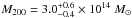
To measure the cluster mass we adopt the usual spherical symmetry and hydrostatic equilibrium assumption, which leads to the simple equation (Sarazin 1988):  (4)The logarithmic derivative of the gas density and temperature profile were computed numerically from our best-fit profiles. When we compute the total dynamical mass profile, we also compute the average density contrast with respect to the critical density at z = 1.03, so that we can solve the equation
 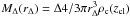 to measure the radius where the average density level is Δ. Typically, mass measurements are reported for Δ = 2500,500,200. Our results are summarized in Table 1. The total mass profile is shown in Fig. 5 (solid line) with the corresponding 68% uncertainty levels. The 1σ confidence intervals on the mass are computed by assuming that the relative errors on the deprojected temperature profile are equal to those on the projected values. Similarly, the relative error on the electron density is equal to half the error on the spectral normalization (therefore at the level of 5% as described above). This is a consequence of the fact that we do not deproject directly the observed profiles, but rather the analytical fitting formulae, therefore we do not introduce additional noise. Clearly the procedure is correct as far as the fitting formulae accurately reproduce the projected profiles. This is a fair assumption, given the large number of free parameters, which allow us to neglect systematic errors associated to the assumed analytical models.
Total cluster mass and gas fraction measured at three radii corresponding to the overdensities of 2500, 500 and 200 with respect to the critical density at redshift z = 1.03.
We remark that we measured temperature and density up to 400 kpc, which is the upper bound of the last bin with significant signal. Beyond this radius, all the derived quantities are obtained by extrapolating the best-fit profiles. As an example, if we assume kT = const. for R > 400 kpc, instead of extrapolating the analytical temperature profiles, we measure 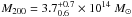 (a value 25% higher). The weak lensing analysis of WARPSJ1415 has been recently published in Jee et al. (2011) using HST/ACS data, yielding a total mass Mtot(r < 1.09 Mpc
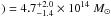 , that is consistent with the X-ray hydrostatic M200 for kT = const. above 400 kpc, and marginally consistent with that obtained with a straight extrapolation. We defer to a forthcoming paper the detailed discussion of the X-ray mass profile of WARPJ1415, as well as independent measurements of the total mass at different radii from a dynamical analysis of all cluster members and the modelling of a strong lensing system.
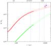 |
Fig. 5 Total mass for WARPJ1415 from hydrodynamical equilibrium (red continuous line) and gas mass (green dashed line). The two dashed lines above and below the total mass profile show the 1σ confidence interval. The profiles are shown with thick lines up to 400 kpc. Thin lines at r > 400 kpc show the extrapolation beyond the X-ray detectable emission. Dashed vertical lines corresponds to R2500, R500 and R200, from left to right. The red data point refers to the mass derived with the global cluster temperature, whereas the blue point corresponds to the weak lensing mass (Jee et al. 2011). |
We also computed the total baryonic mass contributed by the ICM. The mass in baryons is obtained by directly integrating the electron density shown in Fig. 4, assuming the nH = ne/1.2. The measured gas fraction at r500 is 0.10 ± 0.02 (see Table 1 for fb measured at different radii), typical of other distant clusters (see e.g. Ettori et al. 2009).
5. Surface brightness properties, cooling time and entropy
The most immediate observational signature of the presence of a cool-core is a central spike in the surface brightness profile of a cluster. In this section, we use the cluster surface brightness properties to derive several cool-core diagnostics.
5.1. Surface brightness profile
We computed the azymuthally averaged surface brightness profile out to r = 1 Mpc using the vignetted corrected ACIS-S merged image. The isothermal β-model proposed by Cavaliere & Fusco-Femiano (1976) is often used as a simple description of the X-ray surface brightness profiles of galaxy clusters,  (5)where S0, rc, β and C are the central surface brightness, core radius, slope and constant background, respectively. The fitting procedure is based on a Levenberg-Marquardt least-squares minimization and constrains the parameter β to the range 0.4 < β < 1.0. Local cool-core clusters require a double β-model to capture the central emission peak. For distant clusters however, the combination of their intrinsic small angular size and X-ray data that usually provides only low photon statistics, make it difficult if not impossible to distinguish between a single- or a two-component β-model.
Single- and double-β model fit parameters.
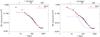 |
Fig. 6 Radial surface brightness profile of WAPSJ1415 (black dots). (Left) Single-beta model fit and (right) double-beta model fit in red solid line. The two components of the double-β model are shown in blue dotted lines. |
We fitted the radial profile of WARPJ1415 using both the single- and double-β model approximations (see Fig. 6). Given the high-quality of our data, we can measure a significant improvement in the fit using the double-beta model, with respect to the single-beta model, not only qualitatively but also statistically – see Table 2 for a list of the fit parameters.
5.2. Surface brightness concentration, cSB
In Santos et al. (2008), we defined the phenomenological parameter cSB that quantifies the excess emission in a cluster core by measuring the ratio of the surface brightness (SB) within a radius of 40 kpc with respect to the average SB within a radius of 400 kpc: cSB = SB(r < 40 kpc)/SB (r < 400 kpc). This simple parameter is particularly useful when dealing with low S/N data. The inner aperture with a physical size of 80 kpc corresponds to the typical size of cool-core clusters regardless of their redshift. We stress that we use a physical radius instead of a scaled radius, since the cool-core phenomenon is non-gravitational in nature, and therefore the self-similar scaling relations are not appropriate in this case.
In Santos et al. (2010), we measured cSB = 0.144 ± 0.016 using the 90 ks ACIS-I observation. The new, more accurate value measured in these deep observations, cSB = 0.150 ± 0.007, is consistent with the previous one.
5.3. Core luminosity excess
Studies of nearby galaxy clusters have estimated that the ICM core contributes to about 25% of the total cluster luminosity (Peres et al. 1998; Best et al. 2007). The method used to compute this luminosity boost was to measure the ratio L(r < rcool)/Lbol. We argue that this is not the most efficient way to isolate the contribution of the cool-core to the luminosity because a fraction of the flux in L(r < rcool) comes from the bulk of the cluster.
To quantify the excess luminosity due to the cool-core, we simply computed the ratio of the flux enclosed by each of the β-model components (core and outer part) at r = 40 kpc (see Table 1). This is the radius used in cSB and is also very close to the crossing of the two β-model components. Following this approach, we estimate that the core contributes 4 times more flux relative to the bulk of the cluster luminosity, at the cooling radius.
The cluster soft-band luminosity within r = 400 kpc is equal to (2.83 ± 0.14) × 1044 erg s-1. We extrapolate this observed luminosity to a radius of 1 Mpc using the single β model, and obtain L(r < 1 Mpc) = 4.0 × 1044 erg s-1 (note that 1 Mpc is about R200 according to our Table 1).
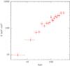 |
Fig. 7 Entropy profile of WARPJ1415 computed from the numerically deprojected temperature and density profiles. |
An accurate assessment of the excess core-luminosity has implications for the completeness of X-ray selected cluster samples. In principle, in a purely flux-limited sample, cool-core clusters are preferentially selected with respect to non cool-core clusters with the same mass, thanks to their higher LX. A proper treatment of this effect will be relevant to properly measure the evolution of cool-cores in future X-ray surveys (see Santos et al. 2011).
5.4. Entropy
Clusters are usually divided in cool-core and non cool-core on the basis of the central value of their entropy and cooling time. However, there are no physical reasons to expect the existence of two distinct populations, in fact the data rather show a transition between these two categories. The specific entropy,  , is a widely used quantity to describe the thermodynamical history of the ICM. Previous studies at low-redshift have shown that cool-core clusters have a significantly lower central entropy (Kc < 30 kev cm2) than non cool-core clusters (Cavagnolo et al. 2008). Using the deprojected temperature and gas profiles as described in Sect. 4, we obtain the entropy profile in Fig. 7.
In order to compare the central gas entropy of WARPJ1415 with the quoted values at low redshift, we have to keep in mind that, since there is no defined radius to perform this measurement, the local measurements are done in very small radii (≤ 1 kpc), whereas our data do not allow us to go below r = 8 kpc. Thus, the central entropy measured in the innermost bin with r = 8 kpc, is Kc = 9.9 ± 2.0 keV cm2, which immediately places WARPJ1415 in the cool-core regime.
Note that the central entropy value obtained from the deprojected profiles refers to a bin centered at 4 kpc, and therefore it is nominally computed at a scale below the actual resolution of our data. We also computed the central entropy at a radius r = 12 kpc as in the first spectroscopic bin, where we actually measured the temperature in the projected data (see Fig. 2, left panel). At r = 12 kpc the projected temperature is kT = 3.8 ± 0.3, and this gives a value of Kc(r = 12 kpc) = 20.9 ± 2.7 kev cm2. This value represents our conservative estimate of the central entropy and it is consistent with a linear relation K(r) ∝ r for r < 40 kpc down to r < 10 kpc.
5.5. Cooling time
The ICM central cooling time is the quantity most often used to characterize and quantify the cool-core strength of a cluster (e.g. Hudson et al. 2010). Without a heating source to compensate radiative cooling, the ICM will radiate its thermal and gravitational energy on a timescale tcool = p/ [(γ − 1)nenHΛ(T)] < 1 Gyr (Fabian & Nulsen 1977), where p is the gas pressure, Λ(T) is the cooling function and γ is the ratio of specific heats of the gas. Adopting an isobaric cooling model for the central gas, tcool can be computed as: 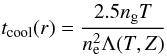 (6)where Λ(T,Z), ng, ne and T are the cooling function, gas number density, electron number density and temperature respectively, with ng = 1.9 ne (Peterson & Fabian 2006). Local cool-core clusters are defined by a central cooling time much shorter than the Hubble time (typically tcool,c ≤ 1 Gyr).
An accurate measurement of the ICM cooling time profile of distant galaxy clusters has been unattainable up to now, due to the use of a single ICM temperature and the average electron density instead of the resolved profiles. With the current data, we are able to trace the precise cooling time profile of WARPJ1415, using the resolved temperature, density and metal abundance profiles. The cooling function Λ(T,Z), was computed using the cooling tables from Sutherland & Dopita (1993) that account for a varying metallicity.
By proceeding similarly to the computation of the central entropy, we obtain a central cooling time tcool ranging from 0.06 ± 0.01 Gyr at r = 8 kpc to 0.23 Gyr at r = 12 kpc (the central bin of our spectroscopic analysis). This accurate measurement is a factor 15 lower than the upper limit of tcool(r < 20 kpc) = 3.4 Gyr obtained by Santos et al. (2010), using the archival data and the global cluster properties. This result clearly demonstrates that, unless deep, high-resolution data of high-z clusters are available, the central cooling time can only be taken as an upper limit.
In Table 2, we summarize the X-ray cool-core properties of WARPJ1415 using the various cool-core diagnostics described above.
X-ray cool-core estimators.
6. Connection between ICM core properties and the BCG
In this paper, we also explore the connection between the radio and optical properties of the brightest cluster galaxy with the ICM cool core properties. Brightest cluster galaxies hold a special place in the history of galaxy formation and evolution. They are the most massive galaxies in the Universe, and are thought to have developed through mergers as expected in a hierarchical assembly model. They are located at the bottom of the potential well of massive clusters and are often coincident with the X-ray peak emission of the hot gas permeating galaxy clusters. The role of the BCG in shaping the ICM properties in the core as a function of cosmic epoch remains unclear, but it is expected to be an important factor in the ICM evolution, playing an important role in the thermodynamical equilibrium of the cool-core.
In the center of cool-core clusters, star formation arises as a result of the cooling process of the ICM (Crawford et al. 1999), with typical star formation rates in their BCGs on the order of 1–10 M⊙/yr (O’Dea et al. 2008). Interestingly, this connection may not be strictly localized in the cluster center, as indicated by McDonald et al. (2010), who found a correspondence between the spatial location of Hα emission regions with the X-ray morphology (un/disturbed) of the ICM core region in nearby systems.
The radio emission of the central galaxy is related to the accretion process onto a supermassive black hole. The incidence rate of radio sources in the center of cool-core clusters is at least 70% (Best et al. 2006; Mittal et al. 2009; Dunn et al. 2008), whereas fewer than 30% of non-CCs host central radio sources. Several studies have established a link between the radio luminosity of these sources with the X-ray and optical properties of their host clusters. In addition, other morphological features such as radio lobes or jets are occasionally detected. At redshift greater than 0.5, interactions between the central galaxy and the ICM remain largely unexplored.
The BCG of WARPJ1415 is very large, luminous and unusually massive, with a reported stellar mass of 2 × 10¹² M⊙ (Fritz et al. 2009). The color image obtained with SUBARU-Suprime Cam BRZ (Fig. 8) shows that the cluster central galaxy stands out as a large, massive red galaxy, and we confirm that the BCG, the central radio source and the peak of the X-ray emission, are spatially coincident well within 1′′. In this section, we analyze the radio and optical properties of the central brightest galaxy, in order to investigate the feedback mechanism between the BCG and the ICM.
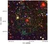 |
Fig. 8 Subaru-Suprime BVR color image of WARPJ1415 covering an area with 2′ × 2′ (~1 × 1 Mpc), centered at RA = 14:15:11, Dec = +36:12:03. North is up and East is to the left. X-ray contours (with levels [3, 5, 10, 20, 30, 50]σ above the background and smoothed with a Gaussian kernel with FWHM = 5″) are overlaid in green. The 15″ × 15″ inset shows the core with a zoom factor of 2. |
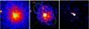 |
Fig. 9 (Left) Chandra full-band image with VLA radio contours overlaid in green. (Middle) Residual Chandra soft-band image after subtraction of the best-fit single β-model. A lack of X-ray emission is observed in sector A with respect to the average surface brightness. This asymmetry is quantified by comparing the average emission in the circular regions labeled 1 and 2 (see text). (Right) VLA image of the radio source coincident with the cluster core. A pronounced extended feature with an extent of 80 kpc is seen in the NW direction. All images have a size of 1′ × 1′. The Chandra images are shown in logarithmic scale with a Gaussian smoothing of 2″. |
6.1. Central radio galaxy and extended structure
WARPJ1415 was observed with the Very Large Array (VLA) of the National Radio Astronomy Observatory in 2002 and 2003 in the A and B configurations at 1.4 GHz (proposal code AP439). The combined radio map, with one hour exposure, has a resolution of 2″ and a noise level of 0.016 mJy/beam. It shows a bright radio source coincident with the X-ray centroid of the cluster and the BCG. Thanks to our high resolution the radio source is resolved in a bright nuclear emission (3.59 ± 0.02 mJy) and a fainter one-sided structure in PA ~ 70° with an extent of ~10″, corresponding to a physical size of 80 kpc at the cluster redshift (see Fig. 9). The flux density of this structure is (0.71 ± 0.05) mJy and therefore the total flux density of the source is 4.3 mJy. Using low resolution NVSS data we estimate a total flux density of about 5 mJy, suggesting that in our high resolution image all the radio source is visible.
The source radio power is in the range between Fanaroff-Riley FR I and FR II radio galaxies, with a total radio power of 2.0 × 1025 W Hz-1 (νLν = 2.8 × 1041 erg s-1). According to the low-redshift study of Sun et al. (2009), all BCGs with a radio AGN more luminous than 2 × 10²³ W Hz-1 at 1.4 GHz are found to have X-ray cool-cores. We also searched for the location of WARPJ1415 in the BCG radio power vs. Kc correlation for clusters with z < 0.2 presented in Cavagnolo et al. (2008) (Fig. 2 of that paper). We find that our cluster falls in the area under the threshold value Kc < 30 keV cm2, and with νLν > 1040 erg s-1, that characterizes nearby cool-core clusters.
The extended, asymmetric radio structure could be interpreted as a mildly relativistic one-sided jet. However this is unlikely, since in relatively low-power radio galaxies jets are relativistic only on a few kpc scale, therefore with a size of ~80 kpc we should expect to detect radio emission also on the other side of the core. No radio lobe seems to be present since the total radio flux density at low resolution is not too far from our high resolution result, and furthermore the structure is resolved also transversally. We may interpret this radio morphology as a tail-like structure due to a strong interaction of extended lobes with the surrounding medium.
Assuming equipartition conditions, we can estimate that in the extended emitting region (~40 kpc) the magnetic field is ~6 μGauss and the minimum non thermal energy is ~3 × 10-12 erg cm-3.
Deeper and higher angular resolution radio data are required to confirm the morphology of the extended radio emission and to provide a direct evidence of a jet-ICM interaction. With the present data, we can only report the tantalizing hint of the feedback mechanism in action in WARPJ1415. However, the high radio power of the central AGN, and the moderate residual star formation estimated in the BCG (see next section) add further evidence in favor of a scenario in which the energy released by the radio loud AGN activity is able to stop the central cooling flow.
6.2. X-ray cavitives?
X-ray cavities originated by outflows of a central radio source are occasionally detected in the ICM of local clusters (e.g. Birzan et al. 2004; Fabian et al. 2006). The detection of such bubbles is challenging even at low redshift due to their low surface brightness contrast and small sizes that range from <1 kpc to ~40 kpc (larger cavities are very rare). Detection rates are of the order of 20–25% in the Chandra archive (Rafferty et al. 2008) and in the flux-limited B55 cluster sample (Dunn et al. 2005). Nearby strong cool-core clusters have a much higher incidence rate, reaching 70%.
Even though we have a deep, high-resolution observation, distant clusters have a small angular size which makes the detection of X-ray cavities very difficult. We searched for X-ray bubbles and/or surface brightness asymmetries that could be associated with the extended radio emission. In order to do this we explored several techniques to improve the image contrast, namely, by subtracting both single and double β-models to the original Chandra soft-band image, and by creating an unsharp-masked image. In the residual images it was difficult to see a convincing indication of a cavity. However, there is a clear asymmetry in the residual image obtained by subtracting the single-β model (see Sect. 5.1) to the X-ray data, with a significant lack of X-ray emission in the upper half of the SB map (labeled sector A in Fig. 9), in the direction of the extended radio emission (green contours). We quantified this asymmetry by measuring the number of net photons in two circular regions with a radius equal to 10′′ in the exposure-corrected Chandra image (see circle 1 and 2 in the middle panel of Fig. 9). The two numbers should be consistent with each other if no asymmetry is present. Instead, we measure 192 ± 14 photons in circle 2 and 153 ± 12 photons in circle 1, showing that region 1 (the one in the direction of the jet) is 25% less luminous with respect to region 2 at a 2-σ confidence level.
6.3. Equivalent width of the [OII] emission line
Optical emission lines (Hα at 6563 Å) are a relatively dust-independent measure of recent star formation. In alternative, the [OII] (λ 3727) emission line is a good proxy for Hα. Brightest cluster galaxies are usually red, early-type galaxies, undergoing passive evolution. Hence, star-formation is seldom found in these central, massive, cluster galaxies. In spite of this, high star formation rates have been found in BCGs of local clusters with central cooling times shorter than ~0.5 Gyr (Rafferty et al. 2008; Cavagnolo et al. 2008), most likely caused by a residual cooling flow.
The brightest central galaxy of WARPJ1415 was observed with the Gemini Multi-Object Spectrograph (GMOS-N, Hook et al. 2004) in 2003 (PI Ebeling). We reduced the archival data with IRAF procedures and obtained the final spectrum, with a scale of 1 Å/per pixel and a resolution R ≈ 1000, as the result of the median stacking of 10 spectra with a total exposure time of 5.3 h and a S/N ~ 5. We expect no major slit loss since the average seeing is 0.7″ and the width of the slit is 1″.
A significant, broad [OII] emission line is found at the cluster redshift. The broadening of optical emission lines originated by warm ionized gas has been often observed in the BCGs of cool-core clusters and is likely a Doppler effect caused by motions in the center of the galaxy (Heckman et al. 1989).
We measured the equivalent width (EW) of the [OII] line defined by  (7)where Fc is the continuum flux and Fλ is the flux of the emission line. The rest-frame EW of the [OII] line in the central galaxy of WARP1415 is –25 ± 3 Å. Our result goes against the interpretation by Samuele et al. (2011) of a strong decrease of star formation activity with redshift, based on the EW of the [OII] line in 77 BCGs selected from the 160 SD survey. In that work, BCGs with an EW stronger than –15 Å are not present. As mentioned in Santos et al. (2010), we suggest that cool-core clusters might be under represented in the 400 SD sample (and hence its subset, the 160 SD sample), which might also explain the lack of strong [OII] lines in the clusters’ BCGs.
6.4. Star-formation rate of the BCG
We estimate the intrinsic [OII] line luminosity assuming E(B − V) = 0.3, using the following relation from Kewley et al. (2004): ![Mathematical equation: \begin{equation} L\rm{[OII]_{\it i}} \left(erg\,s^{-1}\right) = L [OII]_{o} \times10^{0.572} \end{equation}](/articles/aa/full_html/2012/03/aa18162-11/aa18162-11-eq184.png) (8)where L[OII]o is the observed [OII] luminosity. The [OII] line falls in optical i-band at the cluster redshift, therefore we used the high-resolution HST/ACS F775W (i′-band) archival observations to determine the luminosity of the [OII] line. We scaled the observed spectrum to the F775W magnitude of the BCG measured within a radius of 0.75″, in the interval encompassed by the F775W filter.
(8)where L[OII]o is the observed [OII] luminosity. The [OII] line falls in optical i-band at the cluster redshift, therefore we used the high-resolution HST/ACS F775W (i′-band) archival observations to determine the luminosity of the [OII] line. We scaled the observed spectrum to the F775W magnitude of the BCG measured within a radius of 0.75″, in the interval encompassed by the F775W filter.
To derive the galaxy star formation rate, we applied the modified Kennicutt law corrected for reddening as presented in Kewley et al. (2004), considering a mass range of 0.1–100 M⊙ for a Salpeter (Salpeter 1955) initial mass function: ![Mathematical equation: \begin{equation} {\rm SFR \, [OII]}\, (M_\odot \, {\rm yr}^{-1}) = (6.58\pm1.65)\times10^{-42}~L\rm{[OII]}. \end{equation}](/articles/aa/full_html/2012/03/aa18162-11/aa18162-11-eq190.png) (9)Depending on the assumptions made on the amount of dust, we provide a range of SFR. In a dust-free scenario, we estimate SFR = 2.2 M⊙/yr, instead, if we assume a reddening correction of E(B − V) = 0.3, a value typically used in star-forming galaxies (e.g. Lemaux et al. 2010), we obtain SFR = 8.3 M⊙ yr-1.
(9)Depending on the assumptions made on the amount of dust, we provide a range of SFR. In a dust-free scenario, we estimate SFR = 2.2 M⊙/yr, instead, if we assume a reddening correction of E(B − V) = 0.3, a value typically used in star-forming galaxies (e.g. Lemaux et al. 2010), we obtain SFR = 8.3 M⊙ yr-1.
Alternatively, the [OII] line emission in red-sequence galaxies of high-redshift clusters (z ~ 0.9) may be caused by an AGN (Lemaux et al. 2010). Although we cannot entirely rule out emission from an AGN contributing to the estimated star formation rate in WARPJ1415, the fact that we do not detect an X-ray point source coincident with the BCG supports the assumption that the [OII] emission can be entirely ascribed to star formation processes associated to the residual cooling flow in the core. In a forthcoming paper, we will further explore the properties of the BCG and the cluster galaxy population, using a rich optical-IR dataset, including the photometry used here from HST/ACS, SUBARU/Suprime in addition to Spitzer-IRAC. The use of infrared data will allow us to firmly disentangle a possible AGN contamination to the SF rate diagnostics.
6.5. Fe excess and the ICM metal enrichment process
The interplay between the BCGs and their host clusters were first studied by Edge & Stewart (1991). They found a correlation between the optical luminosity of the BCG with the X-ray luminosity and hot gas temperature of its host cluster. This work was expanded by De Grandi et al. (2004), where the excess iron mass in the core region of the ICM has been shown to correlate with the optical and NIR luminosity of the BCG, suggesting a co-evolution between the stellar content of the galaxy and the ICM metal abundance.
We measured a total Fe mass  (within R200) using the best-fit abundance profile (see Sect. 4). For the purpose of our study, it is more interesting to measure the Fe mass excess,
  , following the definition of De Grandi et al. (2004). This is simply the residual iron mass within 200 kpc, obtained by subtracting the almost constant abundance value measured at R > 200 kpc (0.25 Z⊙ in units of Asplund et al. 2005). We measured
  which corresponds to about 30% of the total Fe mass. This number is larger than the average value of 10% found in nearby cool-core clusters studied in De Grandi et al. (2004), but the difference is not significant due to the large scatter in the observed local values. In fact, we find that our cluster lies in good agreement with the correlation between the iron mass excess measured in local cool-cores and their temperature.
To probe the connection between the optical properties of the central galaxy and the metal enrichment of the ICM, De Grandi et al. (2004) found a correlation between the absolute optical magnitude of their local BCGs computed with the Rc-band with the excess iron mass. Assuming that the iron excess is originated entirely by the BCG, this relation may imply that the efficiency of the metal transport mechanisms from the galaxy to the ICM may be approximately the same in all clusters.
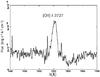 |
Fig. 10 Observed optical GMOS spectrum of the BCG of WARPJ1415 showing a prominent, broad [OII] emission line. |
In order to check whether WARPJ1415 is consistent with this correlation found in local cool-cores, we measured the aperture magnitude of the BCG using the Suprime Rc-band. The k-correction was computed with a SWIRE elliptical template of 5 Gyr, generated with the GRASIL code (Silva et al. 1998). We obtain an absolute magnitude of –23.8 mag, therefore WARPJ1415 falls in the expected  relation for local cool-core clusters (see Fig. 10 of De Grandi et al. 2004). In the assumption that the excess iron mass is entirely due to Type Ia SNe and stellar mass loss in the BCG, we can immediately place an upper limit to the time-scale needed to build up the iron peak. We can safely assume that the bulk of the stars in the BCG formed at about z ≳ 2 (Renzini 2006). We also consider z = 3 as upper limit to the epoch when most of the stars in BCG have formed, as indicated by the observation of major star-formation episodes in massive spheroids at z ≥ 2 (Daddi et al. 2004) or stellar population modeling of high-z BCGs (e.g. Rosati et al. 2009). This corresponds to a lookback time of 10.3 Gyr (11.5 Gyr at z = 3) in the adopted cosmology. Since WARPJ1415 lies at a lookback time of nearly 7.9 Gyr, the build up of its metal peak must have happened on a timescale of ~2.4 Gyr with an upper limit of 3.6 Gyr. Our results point towards times scales shorter than previously claimed (>5 Gyr see Böhringer et al. 2004) to develop a supra-solar iron abundance peak. This would imply a SNe Ia rate larger than expected at z > 1 in the BCG, an evidence which should be compared with the recent first estimate of Type Ia SN rate in high-z clusters (Barbary et al. 2012). In a forthcoming paper (Tozzi et al., in prep.) we will investigate the far reaching consequences these data have on chemical enrichment models, specifically how one can constrain the time scale of the iron production rate through SNe Ia, and the relative contributions of SNe Ia, stellar mass loss and SNII.
7. Conclusions
In this paper we presented a unique Chandra observation of a distant galaxy cluster. These data enabled a spatially resolved analysis of the ICM, with the main goal of studying the properties of the cluster cool-core, and trace a connection with the central galaxy, using optical and radio data. We measured the following X-ray properties:
-
A significant temperature decrease towards the center:Tc = 4.6 ± 0.4 keV, is 2.2 keV lower than the global temperature, T = 6.8 keV and 3.4 keV lower than the maximum temperature at r = 90 kpc, T = 8.0 keV.
-
A surprisingly pronounced metallicity peak,
 with a corresponding excess iron mass
  .
. -
A central surface brightness excess modeled by a double-β model and quantified by cSB = 0.150 ± 0.007. The contribution of the cool-core to the X-ray luminosity within r = 40 kpc is 4 times the value obtained by extrapolating the surface brightness profile from outside the cool-core towards the center.
-
The central cooling time, tcool,c = 0.06 (0.23) Gyr and the central entropy, Kc = 9.9 (20.9) keV cm2 at r = 8 (12) kpc (the values in parentheses correspond to a more conservative estimate).
-
Using the measured temperature and density profiles, the cluster total X-ray mass, under the assumption of hydrostatic equilibrium, is
 .
.
Using VLA high-resolution data we detected a source coincident with the BCG with a radio luminosity L1.4 GHz = 2.0 × 1025 W Hz-1. A faint, one-sided structure with an extent of 80 kpc is seen in the north-west direction, where a significant lack of X-ray emission was found. Furthermore, the analysis of optical spectroscopy of the central galaxy shows a broad [OII] emission line, with a moderate to strong equivalent width of –25 Å, corresponding to an associated star formation rate in the range [2.3–8.3] M⊙/yr.
We were also able to trace a connection between the radio and optical properties of the central galaxy with the X-ray cool-core. By comparing the correlations among the radio luminosity, SFR and Kc measured with low-redshift clusters with our results, we confirm the same feedback mechanism at work in the core of WARPJ1415.
We were also able to investigate the connection between the radio and the optical properties of the central galaxy with those of the ICM properties in the core. In particular, the ratio between radio luminosity, Kc magnitude and the estimated SFR in the BCG of WARPJ1415 is consistent with what is found in low-redshift clusters. These findings suggest that the feedback mechanism at work in the core of WARPJ1415 is of the same kind and intensity of that observed in local clusters.
The prominent Fe peak indicates that the metal enrichment mechanisms by type Ia supernovae (SN Ia) and star formation in the BCG happened on a short timescale (given the lookback time of 7.8 Gyr), and/or that the transport processes that drive away the metals to the outskirts (e.g. galactic winds) were not efficient to smear out the Fe excess.
The analysis of the Chandra data shows that WARPJ1415 at z = 1 has all the classical features that characterize nearby cool-core clusters. These observations enabled the most detailed analysis of the ICM of a z ≥ 1 cluster and our results highlight the importance of deep, high-resolution data to adequately characterize distant clusters. We were able to obtain a noticeable improvement on the previous X-ray characterization and our results set strong constraints on cluster evolution models.
Our results are a first step towards understanding a possible cosmological evolution of the central feedback in galaxy clusters, and refining AGN feedback prescriptions in galaxy evolution models at higher redshifts. To this aim, clearly a sizable representative sample of distant clusters with similar data quality, i.e. S/N and angular resolution, is needed. This is a task which only Chandra can currently achieve, albeit with a substantial investment of time, whereas it is within comfortable reach of next generation wide field X-ray telescopes (e.g., the Wide Field X-ray Telescope, Giacconi et al. 2009). In Santos et al. (2011), we studied how the measure of the parameter cSB varies with redshift and angular resolution using simulated clusters. Based on this study we predict that we will be able to properly evaluate cSB for WARPJ1415 with an angular resolution of 5′′ (Half Energy Width) or better. We conclude that only a combination of a large effective area and a large field of view, when coupled with a constant angular resolution of the order of 5′′, can provide a significant breakthrough on the study of cool-core clusters over a wide redshift range up to z = 1.5, both in terms of statistics and data quality. With current X-ray facilities, we expect that only few cases can be studied with an accuracy comparable to that of WARPJ1415.
The values normalized to Asplund et al. (2005) are a factor 1.6 larger than the ones normalized to Anders & Grevesse (1989) which have been extensively used so far in the literature.
Acknowledgments
We thank Italo Balestra for reducing the XMM-Newton data of WARPJ1415, and Sabrina De Grandi for useful comments on the metal enrichment of the ICM. We also thank the Chandra team for their assistance. This work was carried out with Chandra Observation Award Number 12800510 in GO 12. We acknowledge support under grants ASI-INAF I/088/06/0 e ASI-INAF I/009/10/0. P.T. acknowledges support under the grant INFN PD51.
References
- Anders, E., & Grevesse, N. 1989, Geochim. Cosmochim. Acta, 53, 197 [Google Scholar]
- Arnaud, K. A. 1996, in Astronomical Data Analysis Software and Systems V, ASP Conf. Ser., 101, 17 [Google Scholar]
- Asplund, M., Grevesse, N., & Sauval, A. J. 2005, Cosmic Abundances as Records of Stellar Evolution and Nucleosynthesis, ASP Conf. Ser., 336, 25 [NASA ADS] [Google Scholar]
- Balestra, I., Tozzi, P., Ettori, S., et al. 2007, A&A, 462, 429 [NASA ADS] [CrossRef] [EDP Sciences] [Google Scholar]
- Barbary, K., Aldering, G., Amanullah, R., et al. 2012, ApJ, 745, 32 [NASA ADS] [CrossRef] [Google Scholar]
- Best, P. N., Kaiser, C. R., Heckman, T. M., & Kauffmann, G. 2006, MNRAS, 368, L67 [NASA ADS] [Google Scholar]
- Best, P. N., von der Linden, A., Kauffmann, G., Heckman, T. M., & Kaiser, C. R. 2007, MNRAS, 379, 894 [NASA ADS] [CrossRef] [Google Scholar]
- Bîrzan, L., Rafferty, D. A., McNamara, B. R., Wise, M. W., & Nulsen, P. E. J. 2004, ApJ, 607, 800 [NASA ADS] [CrossRef] [Google Scholar]
- Bîrzan, L., McNamara, B. R., Nulsen, P. E. J., Carilli, C. L., & Wise, M. W. 2008, ApJ, 686, 859 [NASA ADS] [CrossRef] [Google Scholar]
- Blanton, E. L., Sarazin, C. L., McNamara, B. R., & Wise, M. W. 2001, ApJ, 558, L15 [NASA ADS] [CrossRef] [Google Scholar]
- Blanton, E. 2010, in Chandra’s First Decade of Discovery Special Feature edition of the PNAS [arXiv:1004.0671] [Google Scholar]
- Böhringer, H., Matsushita, K., Churazov, E., Finoguenov, A., & Ikebe, Y. 2004, A&A, 416, L21 [NASA ADS] [CrossRef] [EDP Sciences] [Google Scholar]
- Cavagnolo, K. W., Donahue, M., Voit, G. M., & Sun, M. 2008, ApJ, 683, L107 [NASA ADS] [CrossRef] [Google Scholar]
- Cavaliere, A., & Fusco-Femiano, R. 1976, A&A, 49, 137 [NASA ADS] [Google Scholar]
- Crawford, C. S., Allen, S. W., Ebeling, H., Edge, A. C., & Fabian, A. C. 1999, MNRAS, 306, 857 [NASA ADS] [CrossRef] [Google Scholar]
- Daddi, E., Cimatti, A., Renzini, A., et al. 2004, ApJ, 600, L127 [NASA ADS] [CrossRef] [Google Scholar]
- De Grandi, S., & Molendi, S. 2009, A&A, 508, 565 [NASA ADS] [CrossRef] [EDP Sciences] [Google Scholar]
- De Grandi, S., Ettori, S., Longhetti, M., & Molendi, S. 2004, A&A, 419, 7 [NASA ADS] [CrossRef] [EDP Sciences] [Google Scholar]
- Donahue, M., Bruch, S., Wang, E., et al. 2010, ApJ, 715, 881 [NASA ADS] [CrossRef] [Google Scholar]
- Dunn, R. J. H., & Fabian, A. C. 2008, MNRAS, 385, 757 [NASA ADS] [CrossRef] [Google Scholar]
- Dunn, R. J. H., Fabian, A. C., & Taylor, G. B. 2005, MNRAS, 364, 1343 [NASA ADS] [CrossRef] [Google Scholar]
- Dunn, R. J. H., Allen, S. W., Taylor, G. B., et al. 2010, MNRAS, 404, 180 [NASA ADS] [Google Scholar]
- Ehlert, S., Allen, S. W., von der Linden, A., et al. 2011, MNRAS, 411, 1641 [NASA ADS] [CrossRef] [Google Scholar]
- Edge, A. C., & Stewart, G. C. 1991, MNRAS, 252, 428 [NASA ADS] [CrossRef] [Google Scholar]
- Ettori, S., Morandi, A., Tozzi, P., et al. 2009, A&A, 501, 61 [NASA ADS] [CrossRef] [EDP Sciences] [Google Scholar]
- Fabian, A. C. 1994, ARA&A, 32, 277 [NASA ADS] [CrossRef] [Google Scholar]
- Fabian, A. C., & Nulsen, P. E. J. 1977, MNRAS, 180, 479 [NASA ADS] [CrossRef] [Google Scholar]
- Fabian, A. C., Sanders, J. S., Taylor, G. B., et al. 2006, MNRAS, 366, 417 [Google Scholar]
- Foley, R. J., Andersson, K., Bazin, G., et al. 2011, ApJ, 731, 86 [NASA ADS] [CrossRef] [Google Scholar]
- Fritz, A., Jørgensen, I., Schiavon, R. P., & Chiboucas, K. 2009, Astron. Nachr., 330, 931 [NASA ADS] [CrossRef] [Google Scholar]
- Giacconi, R., Borgani, S., Rosati, P., et al. 2009, Astro2010: The Astronomy and Astrophysics Decadal Survey, Science White Papers, no. 90 [Google Scholar]
- Graham, J., Fabian, A. C., Sanders, J. S., & Morris, R. G. 2006, MNRAS, 368, 1369 [NASA ADS] [CrossRef] [Google Scholar]
- Grant, C. E., Bautz, M. W., Kissel, S. E., & LaMarr, B. 2004, Proc. SPIE, 5501, 177 [NASA ADS] [CrossRef] [Google Scholar]
- Heckman, T. M., Baum, S. A., van Breugel, W. J. M., & McCarthy, P. 1989, ApJ, 338, 48 [NASA ADS] [CrossRef] [Google Scholar]
- Hook, I. M., Jørgensen, I., Allington-Smith, J. R., et al. 2004, PASP, 116, 425 [NASA ADS] [CrossRef] [Google Scholar]
- Hudson, D. S., Mittal, R., Repirich, T. H., et al. 2010, A&A, 513, A37 [NASA ADS] [CrossRef] [EDP Sciences] [Google Scholar]
- Jee, M. J., Dawson, K. S., Hoekstra, H., et al. 2011, ApJ, 737, 59 [NASA ADS] [CrossRef] [Google Scholar]
- Jones, L. R., Scharf, C., Ebeling, H., et al. 1998, ApJ, 495, 100 [NASA ADS] [CrossRef] [Google Scholar]
- Kaastra, J. S. 1992, Internal SRON-Leiden Report, updated version 2.0 [Google Scholar]
- Kewley, L. J., Geller, M. J., & Jansen, R. A. 2004, AJ, 127, 2002 [NASA ADS] [CrossRef] [Google Scholar]
- Lemaux, B. C., Lubin, L. M., Shapley, A., et al. 2010, ApJ, 716, 970 [NASA ADS] [CrossRef] [Google Scholar]
- Liedahl, D. A., Osterheld, A. L., & Goldstein, W. H. 1995, ApJ, 438, L115 [NASA ADS] [CrossRef] [Google Scholar]
- Maughan, B. J., Jones, L. R., Ebeling, H., & Scharf, C. 2006, MNRAS, 365, 509 [NASA ADS] [CrossRef] [Google Scholar]
- Maughan, B. J., Jones, C., Jones, L. R., & Van Speybroeck, L. 2007, ApJ, 659, 1125 [NASA ADS] [CrossRef] [Google Scholar]
- Maughan, B. J., Jones, C., Forman, W., & Van Speybroeck, L. 2008, ApJS, 174, 117 [NASA ADS] [CrossRef] [Google Scholar]
- McDonald, M., Veilleux, S., Rupke, D. S. N., & Mushotzky, R. 2010, ApJ, 721, 1262 [NASA ADS] [CrossRef] [Google Scholar]
- McNamara, B. R., & Nulsen, P. E. J. 2007, ARA&A, 45, 117 [NASA ADS] [CrossRef] [MathSciNet] [Google Scholar]
- Menanteau, F., Hughes, J. P., Sifon, C., et al. 2012, ApJ, accepted [arXiv:1109.0953] [Google Scholar]
- Mittal, R., Hudson, D. S., Reiprich, T. H., & Clarke, T. 2009, A&A, 501, 835 [NASA ADS] [CrossRef] [EDP Sciences] [Google Scholar]
- Nousek, J. A., & Shue, D. R. 1989, ApJ, 342, 1207 [NASA ADS] [CrossRef] [Google Scholar]
- O’Dea, C. P., Tozzi, P., Gobat, R., et al. 2008, ApJ, 681, 1035 [NASA ADS] [CrossRef] [Google Scholar]
- Peres, C. B., Fabian, A. C., Edge, A. C., et al. 1998, MNRAS, 298, 416 [NASA ADS] [CrossRef] [Google Scholar]
- Perlman, E. S., Horner, D. J., Jones, L. R., et al. 2002, ApJS, 140, 265 [NASA ADS] [CrossRef] [Google Scholar]
- Peterson, J. R., & Fabian, A. C. 2006, Phys. Rep., 427, 1 [NASA ADS] [CrossRef] [Google Scholar]
- Peterson, J. R., Kahn, S. M., Paerels, F. B. S., et al. 2003, ApJ, 590, 207 [NASA ADS] [CrossRef] [Google Scholar]
- Rafferty, D. A., McNamara, B. R., & Nulsen, P. E. J. 2008, ApJ, 687, 899 [NASA ADS] [CrossRef] [Google Scholar]
- Renzini, A. 2006, ARA&A, 44, 141 [NASA ADS] [CrossRef] [Google Scholar]
- Renzini, A., Ciotti, L., D’Ercole, A., & Pellegrini, S. 1993, ApJ, 419, 52 [NASA ADS] [CrossRef] [Google Scholar]
- Rosati, P., Borgani, S., & Norman, C. 2002, ARA&A, 40, 539 [NASA ADS] [CrossRef] [Google Scholar]
- Rosati, P., Tozzi, P., Gobat, R., et al. 2009, A&A, 508, 583 [NASA ADS] [CrossRef] [EDP Sciences] [Google Scholar]
- Salpeter, E. E. 1955, ApJ, 121, 161 [Google Scholar]
- Samuele, R., McNamara, B. R., Vikhlinin, A., & Mullis, C. R. 2011, ApJ, 731, 31 [NASA ADS] [CrossRef] [Google Scholar]
- Sanders, J. S., & Fabian, A. C. 2007, MNRAS, 381, 1381 [NASA ADS] [CrossRef] [Google Scholar]
- Sanders, J. S., Fabian, A. C., & Taylor, G. B. 2009, MNRAS, 396, 1449 [NASA ADS] [CrossRef] [Google Scholar]
- Santos, J. S., Rosati, P., Tozzi, P., et al. 2008, A&A, 483, 35 [NASA ADS] [CrossRef] [EDP Sciences] [Google Scholar]
- Santos, J. S., Tozzi, P., Rosati, P., & Böhringer, H. 2010, A&A, 521, A64 [NASA ADS] [CrossRef] [EDP Sciences] [Google Scholar]
- Santos, J. S., Tozzi, P., & Rosati, P. 2011, Mem. Soc. Astron. Ital. Suppl., 17, 66 [NASA ADS] [Google Scholar]
- Sarazin, C. L. 1988, Cambridge Astrophysics Series (Cambridge: Cambridge University Press) [Google Scholar]
- Siemiginowska, A., Burke, D. J., Aldcroft, T. L., et al. 2010, ApJ, 722, 102 [NASA ADS] [CrossRef] [Google Scholar]
- Silva, L., Granato, G. L., Bressan, A., & Danese, L. 1998, ApJ, 509, 103 [NASA ADS] [CrossRef] [Google Scholar]
- Sun, M. 2009, ApJ, 704, 1586 [NASA ADS] [CrossRef] [Google Scholar]
- Sutherland, R. S., & Dopita, M. A. 1993, ApJS, 88, 253 [NASA ADS] [CrossRef] [Google Scholar]
- Tozzi, P., Gilli, R., Mainieri, V., et al. 2006, A&A, 451, 457 [NASA ADS] [CrossRef] [EDP Sciences] [Google Scholar]
- Vikhlinin, A., Kravtsov, A., Forman, W., et al. 2006, ApJ, 640, 691 [NASA ADS] [CrossRef] [Google Scholar]
- Voit, G. M. 2005, Rev. Mod. Phys., 77, 207 [NASA ADS] [CrossRef] [Google Scholar]
- Wilms, J., Allen, A., & McCray, R. 2000, ApJ, 542, 914 [NASA ADS] [CrossRef] [Google Scholar]
- Wise, M. W., McNamara, B. R., Nulsen, P. E. J., Houck, J. C., & David, L. P. 2007, ApJ, 659, 1153 [NASA ADS] [CrossRef] [Google Scholar]
All Tables
Total cluster mass and gas fraction measured at three radii corresponding to the overdensities of 2500, 500 and 200 with respect to the critical density at redshift z = 1.03.
All Figures
|
Fig. 1 Folded global spectrum of WARPJ1415 extracted from a circular region with radius of 32″ in the ACIS-S data (crosses) fitted with a mekal model (continuous line). The redshifted Kα line complex of hydrogen-like and helium-like iron (Fe XXV, XXVI) is clearly visible at ~3.5 keV. |
| In the text | |
|
Fig. 2 Left panel: observed projected temperature profile of WARP1415 (red points) and the corresponding fit (red dashed line) compared to the deprojected measured temperature values (blue solid line). Right panel: same as left panel for the iron abundance profile. The 68% uncertainty in the fitted curves is very close to the typical error bars of the measured projected quantities at similar radii, and it is not shown for the sake of clarity. |
| In the text | |
|
Fig. 3 Temperature map obtained in a square region 40″ × 40″ centered on the cluster. The colorbar indicates the temperature scale in keV. Pixels where the 1 sigma error is larger than 50% are masked in black. See text for details. |
| In the text | |
|
Fig. 4 Deprojected electron density profile (red points) and double beta model best fit show in solid blue line. The two individual β model components are shown in dashed lines. |
| In the text | |
|
Fig. 5 Total mass for WARPJ1415 from hydrodynamical equilibrium (red continuous line) and gas mass (green dashed line). The two dashed lines above and below the total mass profile show the 1σ confidence interval. The profiles are shown with thick lines up to 400 kpc. Thin lines at r > 400 kpc show the extrapolation beyond the X-ray detectable emission. Dashed vertical lines corresponds to R2500, R500 and R200, from left to right. The red data point refers to the mass derived with the global cluster temperature, whereas the blue point corresponds to the weak lensing mass (Jee et al. 2011). |
| In the text | |
|
Fig. 6 Radial surface brightness profile of WAPSJ1415 (black dots). (Left) Single-beta model fit and (right) double-beta model fit in red solid line. The two components of the double-β model are shown in blue dotted lines. |
| In the text | |
|
Fig. 7 Entropy profile of WARPJ1415 computed from the numerically deprojected temperature and density profiles. |
| In the text | |
|
Fig. 8 Subaru-Suprime BVR color image of WARPJ1415 covering an area with 2′ × 2′ (~1 × 1 Mpc), centered at RA = 14:15:11, Dec = +36:12:03. North is up and East is to the left. X-ray contours (with levels [3, 5, 10, 20, 30, 50]σ above the background and smoothed with a Gaussian kernel with FWHM = 5″) are overlaid in green. The 15″ × 15″ inset shows the core with a zoom factor of 2. |
| In the text | |
|
Fig. 9 (Left) Chandra full-band image with VLA radio contours overlaid in green. (Middle) Residual Chandra soft-band image after subtraction of the best-fit single β-model. A lack of X-ray emission is observed in sector A with respect to the average surface brightness. This asymmetry is quantified by comparing the average emission in the circular regions labeled 1 and 2 (see text). (Right) VLA image of the radio source coincident with the cluster core. A pronounced extended feature with an extent of 80 kpc is seen in the NW direction. All images have a size of 1′ × 1′. The Chandra images are shown in logarithmic scale with a Gaussian smoothing of 2″. |
| In the text | |
|
Fig. 10 Observed optical GMOS spectrum of the BCG of WARPJ1415 showing a prominent, broad [OII] emission line. |
| In the text | |
Current usage metrics show cumulative count of Article Views (full-text article views including HTML views, PDF and ePub downloads, according to the available data) and Abstracts Views on Vision4Press platform.
Data correspond to usage on the plateform after 2015. The current usage metrics is available 48-96 hours after online publication and is updated daily on week days.
Initial download of the metrics may take a while.