| Issue |
A&A
Volume 539, March 2012
|
|
|---|---|---|
| Article Number | A117 | |
| Number of page(s) | 17 | |
| Section | Extragalactic astronomy | |
| DOI | https://doi.org/10.1051/0004-6361/201118161 | |
| Published online | 02 March 2012 | |
Multiwavelength campaign on Mrk 509
VIII. Location of the X-ray absorber
1
SRON Netherlands Institute for Space Research,
Sorbonnelaan 2,
3584 CA
Utrecht,
The Netherlands
e-mail: This email address is being protected from spambots. You need JavaScript enabled to view it.
2
Sterrenkundig Instituut, Universiteit Utrecht,
PO Box 80000, 3508 TA
Utrecht, The
Netherlands
3
Mullard Space Science Laboratory, University College
London, Holmbury St. Mary,
Dorking, Surrey,
RH5 6NT,
UK
4
Department of Physics, Virginia Tech, Blacksburg, VA
24061,
USA
5
Department of Physics, Technion-Israel Institute of
Technology, 32000
Haifa,
Israel
6
Dipartimento di Fisica, Università degli Studi Roma
Tre, via della Vasca Navale
84, 00146
Roma,
Italy
7
INAF – IASF Bologna, via Gobetti 101, 40129
Bologna,
Italy
8
Space Telescope Science Institute, 3700 San Martin Drive, Baltimore, MD
21218,
USA
9
Department of Physics and Astronomy, The Johns Hopkins
University, Baltimore, MD
21218,
USA
10
ISDC Data Centre for Astrophysics, Astronomical Observatory of the
University of Geneva, 16 ch.
d’Ecogia, 1290
Versoix,
Switzerland
11
UJF-Grenoble 1/CNRS-INSU, Institut de Planétologie et
d’Astrophysique de Grenoble (IPAG) UMR 5274, 38041
Grenoble,
France
12
School of Physics and Astronomy, University of
Southampton, Highfield, Southampton
SO17 1BJ,
UK
13
Instituto de Astronomía, Universidad Católica del
Norte, Avenida Angamos 0610,
Casilla 1280, Antofagasta, Chile
14
Department of Physics, University of Oxford,
Keble Road, Oxford
OX1 3RH,
UK
Received: 27 September 2011
Accepted: 19 December 2011
Abstract
Aims. More than half of all active galactic nuclei show strong photoionised outflows. A major uncertainty in models for these outflows is the distance of the gas to the central black hole. We use the results of a massive multiwavelength monitoring campaign on the bright Seyfert 1 galaxy Mrk 509 to constrain the location of the outflow components dominating the soft X-ray band.
Methods. Mrk 509 was monitored by XMM-Newton and other satellites in 2009. We have studied the response of the photoionised gas to the changes in the ionising flux produced by the central regions. We used the five discrete ionisation components A–E that we detected in the time-averaged spectrum taken with the RGS instrument. By using the ratio of fluxed EPIC-pn and RGS spectra, we were able to put tight constraints on the variability of the absorbers. Monitoring with the Swift satellite started six weeks before the XMM-Newton observations. This allowed us to use the history of the ionising flux and to develop a model for the time-dependent photoionisation in this source.
Results. Components A and B are too weak for variability studies, but the distance for component A is already known from optical imaging of the [O iii] line to be about 3 kpc. During the five weeks of the XMM-Newton observations we found no evidence of changes in the three X-ray dominant ionisation components C, D, and E, despite a huge soft X-ray intensity increase of 60% in the middle of our campaign. This excludes high-density gas close to the black hole. Instead, using our time-dependent modelling, we find that the density is very low, and we derive firm lower limits to the distance of these components. For component D we find evidence for variability on longer time scales by comparing our spectra to archival data taken in 2000 and 2001, yielding an upper limit to the distance. For component E we derive an upper limit to the distance based on the argument that the thickness of the absorbing layer must be less than its distance to the black hole. Combining these results, at the 90% confidence level, component C has a distance of >70 pc, component D is between 5–33 pc, and component E has a distance >5 pc but smaller than 21–400 pc, depending upon modelling details. These results are consistent with the upper limits that we derived from the HST/COS observations of our campaign and point to an origin of the dominant, slow (v < 1000 km s-1) outflow components in the NLR or torus-region of Mrk 509.
Key words: galaxies: active / X-rays: general / X-rays: galaxies / galaxies: individual: Mrk 509 / quasars: absorption lines
© ESO, 2012
1. Introduction
It has been known for a long time that accretion onto a super-massive black hole plays a key role in the physics of active galactic nuclei (AGN). While outflows have already been detected using early optical observations of NGC 4151 (Anderson & Kraft 1969), their widespread occurrence and role was only recognised after high-resolution UV spectrographs became available. Crenshaw et al. (1999) found that 60% of all Seyfert 1 galaxies show UV absorption lines. While intrinsic X-ray absorption had already been found in the early 1980s, including the first evidence of absorption from ionised gas (Halpern 1984), the proof that this gas is outflowing came from the first high-resolution X-ray spectrum of a Seyfert galaxy (Kaastra et al. 2000). We refer to Crenshaw et al. (2003) for a more extensive overview of outflows.
Measurements of absorption line spectra yield reliable information on different aspects of the outflow such as dynamics (through the Doppler shifts and line profiles) and ionisation state (through intensity ratios of lines from different ions). However, they do not provide a key ingredient, the distance r of the absorbing material to the central black hole. The basic problem is that the ionisation state is described by the parameter ξ = L/nr2 with L the ionising luminosity between 1–1000 Ryd and n the hydrogen density. With L and ξ known from observations, only the product nr2 is known. This degeneracy has led to considering many different locations for the outflow, including the halo of the host galaxy (10 kpc), the inner galactic disc (0.1–1 kpc), the narrow emission line region (10–500 pc), and the intermediate line region (0.01–10 pc). The recently discussed, so-called ultra-fast outflows (see e.g. Tombesi et al. 2010, and references therein) may be even further inwards.
There are several methods of estimating r. The most direct and easiest method is to use direct imaging. A good example are the Doppler maps of [O iii] λ5007 by Phillips et al. (1983) in Mrk 509. However, this method can only be applied for the most nearby sources and for the most extended low-ionisation gas. Instrumental capabilities are insufficient to resolve more centrally concentrated gas.
Other methods rely on obtaining the density n and deriving the distance r through using the ionisation parameter. The most direct way is to use density-sensitive lines from meta-stable levels. This method has been applied in a few cases using different UV lines from meta-stable levels in various sources. The published results display a broad range of distances for different sources, from <0.1 pc (Kraemer et al. 2006), 25 pc (Gabel et al. 2005) to 3 kpc (Moe et al. 2009). In X-rays, Kaastra et al. (2004) pioneered this method theoretically using K-shell absorption lines from O v, but owing to the limited signal from the target that was studied, Mrk 279, they could not obtain firm detections of these lines. For X-ray binaries, however, metastable lines have been found in GRO J1655–40 (Miller et al. 2008), but they sample a density range (~1020 m-3) that is too high for AGN.
Alternatively, variations in the ionising luminosity of an AGN will induce changes in the ionic composition of the surrounding gas, hence changes in the transmitted spectrum. How fast the gas responds depends on the recombination time scale, which is a function of density (for absorption the light-crossing time is not relevant). By measuring the delay (or lack of delay) of an absorption component relative to the luminosity variations, this recombination time scale can be determined and from that the density n and distance r are deduced. The method has been applied to several sources, again yielding a broad range of distances (see for references our introduction in Paper I of this series, Kaastra et al. 2011a).
In this paper we follow the last method. In 2009 we performed a large multiwavelength campaign on one of the best targets for this study, Mrk 509 (Kaastra et al. 2011a). The source has a typical variability time scale of a few days, with sufficiently large amplitude. The first step of our analysis was to characterise the time-averaged properties of the absorber using the combined RGS spectrum of all observations taken by XMM-Newton during our campaign. This has been described in detail by Detmers et al. (2011). Using the multiwavelength monitoring as described by Kaastra et al. (2011a), it is then possible to predict the variations of the transmission of the outflow for a grid of possible distances r. Comparing these predictions with the observed spectra then yields distances to the outflow components. In our comparison, we have focussed on the data obtained with the pn camera of XMM-Newton, because that has the highest sensitivity to variations in the 1 keV band. The MOS data could not be used for this comparison because of a small amount of pile-up. However, we also obtained useful constraints from the RGS spectra at longer wavelengths.
The structure of this paper is as follows. First we summarise the ionisation structure of the outflow, investigate the spectral signatures of the expected variations of the transmission, and introduce the data sets that we use (Sect. 2). As a next step (Sect. 4) we compare the data to the predictions for the high-density limit (instantaneous response of the absorber to continuum variations). Afterwards we describe our method of treating the more general case of time-dependent photoionisation (Sect. 5). In Sect. 6 we compare the data from our 2009 campaign to archival data to obtain constraints from the long-term variability. We discuss our results briefly in Sect. 7.
We use 1σ (68% confidence) uncertainties throughout this paper, unless stated explicitly otherwise.
2. Data
2.1. Fluxed spectra
We have made fluxed spectra for each of the ten observations as well as for the combined spectrum for each of the instruments available to us. The need to use fluxed spectra is explained in more detail in Sect. 3 and is related to the weakness of the expected signals. More details about the observations and the observation log are described by Kaastra et al. (2011a).
2.1.1. EPIC pn spectra
The pn (Strüder et al. 2001) count spectra were extracted as described by Ponti et al. (in prep.). We have produced fluxed spectra from these count rate spectra using the program epicfluxer that is available in the public SPEX1 distribution. Our procedure is as follows. We rebin the count spectra energy-dependent to about 1/3 FWHM, ignore the parts below 0.2 keV and above 12 keV, and fit the count spectra using a cubic spline (the spln model of SPEX) on a logarithmic energy grid between 0.2–12 keV with 100 grid points. The resolution of this grid is about 2%, and it matches the spectral resolution of pn well. All fits are statistically acceptable. We then take the corresponding model photon spectra (also as splines) and convolve them with a Gaussian redistribution function. The FWHM of this Gaussian is energy-dependent and corresponds to the spectral resolution of the instrument at each energy. In this way we have a model spectrum at EPIC resolution that describes the data perfectly. Any remaining residuals that are visible in a plot of the original fit to the count spectra with the spln model, come mostly from the statistical noise of the data. To take that noise into account and also to correct for any remaining weak residuals caused by the limitations of the spline photon spectrum approximation to the true photon spectrum, we scale the convolved spline model spectra with the ratio of the observed data to the predicted data at each energy.
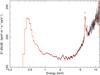 |
Fig. 1 Fluxed pn spectrum for the co-added 2009 spectrum of Mrk 509. The spectrum has been multiplied by E2 for clarity in the display. |
Figure 1 shows an example of the fluxed spectrum of the combined 2009 data. For our analysis we used the data points, but the plot shows the excellent agreement between the response-convolved spline model and the data. The spectrum clearly shows the Fe-K line near 6.4 keV, as well as a dip caused by the absorbing outflow between 0.8 and 1.0 keV. Some of the features between 1.8 and 4 keV may be caused by remaining small calibration uncertainties at a level of a few percent, and are possibly associated to the gold edge of the mirror or the silicon edge of the detector. However, whether these features are instrumental or have an astrophysical origin is not important for the present purpose, as they disappear in the ratio of different spectra. Below 0.4 keV the flux drops rapidly owing to the Galactic absorption. Since the spectral energy resolution in that region of the spectrum is low anyhow and we do not expect to see significant variations in the absorption components in that band, it is not important for the present paper, so we ignore the spectrum below 0.5 keV in the rest of the paper.
Furthermore, we take the following into consideration. Figure 2 shows the ratio of the nominal count spectrum (counts s-1 keV-1) divided by the nominal effective area at each energy, to the fluxed spectrum produced by the epicfluxer program as described above. In particular, at lower energies most of the counts correspond to redistributed photons of higher energies. Because the intrinsic photon spectrum becomes weak at low energies owing to interstellar absorption, the strong rise of the ratio below 0.35 keV, up to ~4 for E = 0.2 keV, is produced. The negative dip around 0.45 keV is caused by loss of photons of 0.45 keV to counts at energies below 0.45 keV.
In the data, an excess of 1% above the model at 0.5 keV would actually be an excess of 1% counts. With the ratio of ~0.9 at 0.5 keV from Fig. 2, this corresponds to an excess in flux of about 1.1%. Our procedure would thus give a systematic bias of 0.1% for the above example. However, the typical statistical uncertainty of the spectra in this region is much smaller than the 1% of the example (<0.4–0.5%). Furthermore, the statistical deviations for neighbouring bins are independent and can have different signs, so their average value over a certain band of bins is even lower. We conclude that these effects on our analysis can be ignored safely.
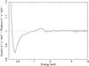 |
Fig. 2 Ratio of the “fluxed” pn count spectrum to the fluxed photon spectrum of Mrk 509. |
The pn is known to be extremely stable over time. Here we quantify this. Stability can only be measured using unvarying sources. Such sources are relatively rare, but perhaps the best candidate is the isolated neutron star RXJ 1856.6–3754. This object is being used as a regular calibration target for XMM-Newton. The best band for checking stability is the 0.3–0.5 keV band, given the soft spectrum of the source. We use the products that are available with the calibration review tool on the XMM-Newton web page. The 15 pn observations of this source in the 0.3–0.5 keV band have fluxes with a standard deviation of 3.8% around the mean value. We are more interested in relative differences rather than absolute fluxes, so we have also determined the mean and standard deviation for the fit residuals averaged over a 0.05 keV wide band around 0.3 keV. These residuals have a mean value of 2.4% (consistent with the nominal calibration uncertainty), but more importantly the scatter (standard deviation) for individual observations around this mean is only ~0.5%. The true number may be even smaller because this number agrees fully with the uncertainty due to the photon statistics in this band (it is limited by the exposure times of the calibration observations). The number implies that relative time variations in narrow bands can be measured down to the ~0.5% level or better, provided the source has enough photons.
2.1.2. EPIC MOS spectra
The MOS (Turner et al. 2001) data cannot be used for our purpose. In contrast to the pn data, the ratios between MOS spectra often show weak breaks around 0.7 keV, with deviations below that energy from the extrapolated power law from the 0.7–1.5 keV band and also deviations from the ratio obtained from the simultaneous pn data. This is caused by a combination of small amounts of pile-up, small imperfections in the MOS redistribution function at low energies, and uncertainties near the instrumental oxygen edge. This softening or hardening near 0.7 keV makes detection of the expected narrow Gaussian differences in transmission harder, because at least for the ionisation components C and D, the centroids of the Gaussians are near this energy (0.716 and 0.820 keV, Table 2). The signal-to-noise ratio of the combined MOS data in the relevant band is also about two times lower than for the corresponding pn data. This is partly due to the smaller extraction radii for the MOS spectra (20′′) as compared to the pn spectra (45′′). For these reasons we do not include the MOS data in our subsequent analysis.
2.1.3. RGS spectra
The data reduction of the RGS (den Herder et al. 2001) spectra was described in detail by Kaastra et al. (2011b). The spectra were taken in the so-called multi-pointing mode. For each observation, one of five offset pointings in the dispersion direction was chosen. This has the advantages that (i) the effects of spectral bins with lower exposure from the excision of bad pixels is strongly reduced in the stacked RGS spectrum; and (ii) that the gaps between CCDs are filled with data. For individual spectra, this advantage is lost, although it is partly recovered by the combination of RGS1 and RGS2 data and first- and second-order spectra.
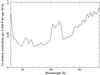 |
Fig. 3 1σ relative uncertainty on the individual ~60 ks RGS spectra of Mrk 509 per 0.058 Å bin. |
We are searching for variation in the depth of absorption lines, so we have rebinned our spectra by a factor of 6 to 0.058 Å, approximately the resolution (FWHM) of the RGS. In Fig. 3 we show our sensitivity to detecting changes in individual RGS spectra. The curve is derived from a 50-point spline fit to the median statistical uncertainties of the ten individual spectra. It ranges between 3 and 6% in the 10–30 Å band, with some maxima (7–9%) at the two ends of the band and in correspondence with the missing CCDs.
3. Description of the outflow and analysis method
3.1. Ionisation structure of the outflow
The time-averaged RGS spectrum of Mrk 509 as analysed by Detmers et al. (2011) shows a number of discrete ionisation components, labelled A–E (see Table 1, taken from the absorption measure distribution fit). The discrete nature of these components could be proved – at least for components C and D – by applying a continuous model for the column density versus ionisation parameter ξ. That continuous model shows two strong peaks in absorption measure at the position of components C and D. The statistics of the spectrum and the lack of suitable strong lines did not allow us to prove the discrete nature of components A, B, and E, but there is also no strong evidence against the discrete nature of these components, so for our present analysis we started with the five components given by Detmers et al. (2011). We use the parameters from his Table 6, given here in Table 1, which is based on a fit of the measured ionic column densities co-added over all velocities resulting in five ionisation components.
Ionisation components used in the present analysis.
Alternatively, Detmers et al. (2011) also fitted the spectrum directly with the xabs model of SPEX (Kaastra et al. 1996) using multiple discrete ionisation and velocity components. In that analysis, component C is split over two velocities (− 40 and −270 km s-1), with slightly different ξ-values (see Table 5 of Detmers et al. 2011). In our discussion we come back to this issue in the context of discussing the uniqueness of our results.
3.2. Transmission of the five components
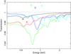 |
Fig. 4 Transmission for the five ionisation components A–E at the resolution of the pn instrument (solid lines). Dotted lines: the same but for log ξ0.1 dex higher. Dashed lines: ratios of the transmission for the higher of the above ionisation states to the lower ionisation states. We use the same colour coding for each component. |
As a starting point in our analysis, we calculated the transmission, convolved with the resolution of the pn detector and with the cosmological redshift applied, for all five individual ionisation components. We focus here on the pn data because of its higher sensitivity at higher energies, but later we also consider the RGS spectra. Because Mrk 509 shows variations of 20–25% in luminosity (~0.1 dex), we also calculated the transmission for these components using the same total hydrogen column density but with log ξ 0.1 dex higher (recall ξ = L/nr2). For other, not too large variability amplitudes we can easily scale these calculations. The results are shown in Fig. 4. This figure also shows the relative change for each component if the ionisation balance is adjusted, by plotting the ratio between the transmission for both cases.
The figure shows that – at the pn resolution – all components show deviations from unity in the transmission, up to 6% for component C. However, the differences in the transmission between the two cases are smaller than the deviations from unity, and they do not always peak at the energy of the dominant absorption features. For instance, component D has the strongest absorption blend at an energy of 0.90 keV, but by increasing the ionisation parameter the main effect is to reduce the depth of the low-energy wing of the blend, resulting in a peak of the difference spectrum at 0.82 keV.
In general ions that have their peak concentration exactly at the ionisation parameter of one of the detected ionisation components, thereby making the strongest contribution to the absorption, are not very sensitive to modest changes in the ionisation parameter, since the second derivative of the ionic column density versus ionisation parameter is close to zero. Therefore, changes in the individual components can be spotted most easily using ions that peak near the relevant ionisation parameter (to yield significant column densities and absorption features), but not exactly at this ionisation parameter (and therefore have a strong gradient of the derivative of the column density versus ξ).
Approximation with Gaussian components of the changes in transmission due to an increase of 0.1 dex in log ξ.
We found that the prominent peaks due to a change ΔT in the transmission for components C, D, and E are represented well by Gaussians: 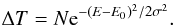 (1)The parameters for these Gaussians (for an increase of 0.1 in log ξ) are given in Table 2.
We discuss the different components in more detail below. Although they affect the transmission below 1 keV at the 1–2% level, components A and B are expected to show changes in the transmission (for an increase in log ξ by 0.1) no larger than 0.1%, so cannot be used for the present purpose of constraining the spectral variations of the absorption components. This lack of sensitivity is due to the lower column densities for these low-ionisation components, combined with the poor spectral resolution of EPIC at low energies, causing relatively strong broadening of spectral lines.
Strongest contributions to the dominant absorption troughs for components C, D, and E.
For this reason we concentrated on components C, D, and E. In their expected response to changes in the ionisation parameter, they show significant features with amplitudes of about a percent at energies of 0.716, 0.820, and 1.056 keV, respectively. Using our spectral model, we estimated the equivalent widths of the lines from all ions that contribute to these features. The results are shown in Table 3.
The expected changes in component C are dominated by the declining column densities of Fe ix–Fe xii as a function of ionisation parameter, and also by the Rydberg series of O vii starting from n = 3. The 1s–2p line of this ion is well separated from the presently considered blend. At the far blue side of the profile, the increase in Fe xvii column density enhances the contrast for these column densities of Fe ix–Fe xii slightly. The dominant lines from Fe xv–Fe xvii are separated reasonably well in energy from the more lowly ionised ions, and thus do not contribute much to the central regions of the blend. As a result, mainly the changes in Fe ix–Fe xiv and O vii and O viii for this component are relevant.
Below 0.715 keV a reduction in the optical depth τ of the O vii edge is also visible (Fig. 4). It decreases from 0.0112 to 0.0079, causing the transmission above the edge to increase by 0.33% relative to the lower energies.
For component D, the O viii 1s–2p line, although it is the strongest line in this energy band, does not contribute significantly to the main component of the variation, because it is 150 eV off the centroid and because the optical depth is large (2.2), causing moderate saturation effects, hence less sensitivity to column density variations. We have included Fe xx for component D in Table 3, because this ion is expected to increase its column density as a response to an increase in ionisation parameter, resulting in a shift of the centroid of the varying transmission component to slightly lower energies.
The changes in component E are dominated by decreasing column densities of Fe xxi–Fe xxiv as a function of ionisation parameter. Component E is also predicted to have a strong absorption feature in the Fe-K band, mainly due to Fe xxv. At EPIC resolution, this line has a maximal depth of about 5%. Because it is possibly blended by emission features of the same ion, it is not possible to measure its equivalent width. If component E responds to the continuum changes, then the line’s peak intensity will change by about 1%, which is too small to detect since the signal-to-noise ratio per observation and per resolution element (FWHM) is only 50 at those high energies. Therefore we do not consider the Fe-K band further here.
For component E, there is a significant uncertainty of 0.27 in the value of log ξ for the time-averaged spectrum as determined by Detmers et al. (2011). This is because of a strong correlation between the total hydrogen column density and ξ. The consequences of this on our analysis are discussed in more detail in Sect. 7. For components C and D, the uncertainties are much smaller. However, because we use in this paper changes relative to the time-averaged spectrum, uncertainties in the absolute values of ξ and NH for the time-averaged spectrum are less important.
3.3. Measuring transmission changes of the outflow
The continuum flux during the XMM-Newton campaign of Mrk 509 varied significantly at a level of the order of 25%, corresponding to 0.1 dex, in the hard X-ray band (Kaastra et al. 2011a). In the soft X-ray band we even see enhancements up to ~60% (see Fig. 12 later in this paper). If any of the ionisation components of the outflow responds rapidly to the changing ionising continuum, then we expect to see the changes in the spectrum as displayed in Fig. 4. If on the other hand the response time is slow, no changes in the transmission may occur. Figure 4 shows that the expected peaks for components C, D, and E are well separated in energy, implying that the (lack of) variations can be detected for each of these components individually.
The amplitude of the expected signal is of the order of 1%. This is smaller than the typical systematic uncertainty in the EPIC effective area, which is a few percent or even slightly larger, and varies with energy. As a result small differences in the model photon spectra cannot be distinguished from imperfections in the adopted effective area. Therefore, global spectral fitting of individual spectra at this level of accuracy is not possible. However, the pn detector of XMM-Newton is extremely stable (Sect. 2.1.1), and therefore relative changes in the spectrum are much easier to detect.
We proceed as follows. We produce fluxed spectra Si for all ten individual observations (i = 1,...10) as described in the next subsection. The ratios rij,obs = Si/Sj of these fluxed spectra are then independent of any effective area uncertainties. Also, in this way the effects of interstellar absorption are taken out. The expected ratio is rij,pred = CiTi/CjTj, where Ci is the intrinsic continuum for spectrum i and Ti the transmission of the absorbing component(s). If there is no change of the absorber, rij,pred is just the ratio of the model continuum spectra. In order to take out the time variability of the continuum, we use instead  (2)and compare this with
  (3)If any of the absorbing components varies over time, Rij,pred and the corresponding Rij,obs will differ from zero in narrow energy bands, cf. our findings in Sect. 3.2.
4. Searching for variations in the outflow in the high density limit
In the previous section we described the structure of the outflow, indicated the characteristic predicted variations as a response to changes in the ionising radiation, and presented the data products that we use to measure these variations.
In our analysis we use three levels of sophistication. At the most simple level we assume that the ionising continuum varies only in flux, but not in shape. In the case of high density, this causes an immediate response to the flux variations with the characteristic signatures as presented in Fig. 4. For gas at a fixed density and distance to the ionising source, a change of L is then directly proportional to a change in ξ.
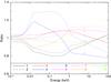 |
Fig. 5 Ratio of the ten model spectra to the time-averaged model spectrum, based on the fits by Mehdipour et al. (2011). Only the underlying continua are taken into account, not the absorption components. The spectra as displayed are extrapolated outside the XMM-Newton range for illustrative purposes. |
However, the above situation is not realistic, Mehdipour et al. (2011) have shown that there are significant changes of the spectral shape during our campaign (Fig. 5, Sect. 4.1). Therefore in this section we study a model where the gas has a high density and hence responds immediately to variations in the ionising flux, but we take the variations in spectral shape as measured simultaneously with the EPIC and OM instruments of XMM-Newton into account. This is an important limit for the more general model of time-dependent ionisation at lower densities that we discuss in Sect. 5.
4.1. Ionising continuum
We follow Mehdipour et al. (2011), who model the continuum as the sum of four components: a disc blackbody (dbb), a soft excess parametrised by a Comptonised disc component (se), a power law (pl) and an Fe-K line (fe, see their Table 5). The iron line does not contribute much to the ionising flux, but for consistency with the fits by Mehdipour et al. (2011) we include it in our model. However, we ignore the weaker narrow and broad X-ray emission lines that are modelled by Detmers et al. (2011) in the soft X-ray band. Those lines also have a negligible contribution to the ionising flux. More details about the model components are given in Sect. 5.2, where we discuss the time-dependent parameters of the components.
The 10log of the ionising (1–1000 Ryd) flux for the ten individual spectra 1–10 divided by the corresponding flux for the time-averaged spectrum, for each of the spectral components as modelled by Mehdipour et al. (2011).
For each of the ten spectra, we have made runs with Cloudy (Ferland et al. 1998) version C08.00 with Lodders et al. (2009) abundances for a grid of ξ-values to calculate the equilibrium ion concentrations. The auxiliary program xabsinput in the public SPEX distribution then converts this into an input file for the xabs model of SPEX. The xabs model was used in the analysis of the time-averaged RGS spectrum by Detmers et al. (2011). For each spectrum we also calculate the ionising luminosity L in the 1–1000 Ryd band (Table 4).
4.2. Predicted and observed changes in transmission: pn
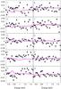 |
Fig. 6 Data points with error bars: observed ratios of the ten spectra (labelled 1–10) to the average spectrum in the representation of Eq. (2) (essentially the spectral ratios with the respective continua divided out and unity-subtracted). Solid green lines: predicted ratio in the representation of Eq. (3) for ionisation component C; dashed blue lines: same for component D; dotted red lines: same for component E; thick magenta line: components A–E combined. The predictions for components A and B are close to zero and not shown here separately. |
As a next step, we calculated for each of the five ionisation components A–E the transmission using the above appropriate SEDs. We also increased or decreased ξ proportionally to the change of the total L from the last column of Table 4. The ratios of the ten transmissions to the time-averaged transmission are then represented using Eq. (3) and compared to the observed pn data using Eq. (2). We show this comparison in Fig. 6.
Observations 4 and 5 show some broad-band residuals in the form of a positive trend between ~0.8 keV and 1.5 keV, while observation 8 shows the opposite trend. A similar bending is seen for these spectra in the plot of the ratio of the model spectra (Fig. 5). These three spectra have their largest curvature just around 1 keV. Thus, the systematic trends in spectra 4, 5 and 8 can be attributed to imperfect continuum modelling. Note that their amplitude of ~1% is well below the systematic uncertainty of the pn effective area calibration. But of course also the continuum models that we use may be too simple at this level of accuracy.
To corroborate this result, we have inspected the fit residuals of the broad-band fits to the ten spectra made by Mehdipour et al. (2011). Averaged over the 1.0–1.5 keV band, the fit residuals of the pn for spectra 4 and 5 are ~0.8% higher than for spectra 2, 9 and 10. Similarly, for observation 8 the fit residuals are ~0.4% smaller than for spectra 2, 9 and 10. Within 0.1%, these differences agree with what we show in Fig. 6. Thus, the large-scale residuals are caused by small imperfections in the continuum modelling of the individual spectra. Recall that the ratios shown in Fig. 6 are essentially the ratios of the observed or predicted photon spectra, but normalised to the corresponding ratio of the pure continuum models obtained by Mehdipour et al. (2011). In contrast to these broad-band trends, the signatures of a varying absorber should be narrow dips or bumps at specific energies, which differ for each of the absorption components (cf. Fig. 4).
The predicted difference in transmission for components A and B is less than ±0.02 and ±0.2%, respectively, and because we are not sensitive enough to detect such weak signals, we will not consider components A and B further. We recall that the sensitivity to detecting changes in narrow energy bands with pn is ~0.5% or slightly better, cf. Sect. 2.1.1.
Component C has the strongest predicted signals. Spectrum 1, and to some lesser extent also spectrum 2, should have a dip with an amplitude of ~−1% at 0.73 keV, while spectrum 5 should have a positive excess with similar amplitude. None of this is visible in the data. However, the predicted dip for spectrum 1 might be visible in spectrum 5, while the predicted bump for spectrum 5 might be visible in spectrum 8. That would correspond to a delay of about two weeks. The possibility of a delayed response, corresponding to lower density and hence more distant gas will be elaborated further in Sect. 5, but we conclude here that the pn data are clearly inconsistent with an immediate response of component C to continuum variations.
The predicted changes for component D are too small to be detectable with pn. This is somewhat surprising because from Fig. 4 one might conclude that the predicted variations should have about half the amplitude of the variations in component C. However, in Fig. 4 it was assumed that the luminosity variations are achromatic, while in the present model we take the more realistic continuum shape variations into account. Because the soft X-ray flux varies more strongly than the hard X-ray flux, the predicted amplitudes for the more highly ionised components D and E are smaller than that of component C. The strongest predicted dip, −0.35% around 0.82 keV for spectrum 1, is comparable to the statistical uncertainty of 0.3% in that band, hence not detectable.
For component E, our model predicts a dip of −1.6% for spectrum 4 at 1.06 keV, in contrast to a positive peak at the same energy of ~+0.5% for spectra 6, 8, and 10. There is not much evidence of the dip in spectrum 4, although some care should be taken because of the small systematic trends noticed earlier for this spectrum, related to the strong curvature of the underlying continuum.
4.2.1. Nominal significance of the variations
The significance of our findings is somewhat difficult to assess quantitatively, due to the small systematic continuum deviations mentioned earlier. We have attempted to quantify this in the following way (Table 5). We calculated the nominal χ2 of the data Robs shown in Fig. 6 compared to two models. The first model (labelled “zero model”) in the table compares the data to the model where the change in transmission is zero (Rpred = 0 in terms of Eq. (3)). This corresponds formally to the limit for the gas density n → 0. We also calculated χ2 for the models with instantaneous response for components C, D, and E (the green, blue and red curves in Fig. 6). This corresponds formally to n → ∞. For comparison with the zero model we subtract χ2 for that model, thus showing the difference in χ2. We do this for each individual observation. The table clearly shows that the model with no response at all is better than the models with an instantaneous response of the absorption components. The numbers agree with what we described qualitatively before. While the sensitivity to detecting changes in component D is low, an instantaneous response for component C would make the total χ2 25.4 higher than the zero model. An almost similar conclusion can be drawn for component E.
Comparison of the 10 spectra with models for the change in transmission.
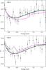 |
Fig. 7 Example of continuum adjustment for spectra 4 (top panel) and 5 (bottom panel). Data points with error bars: observed ratio of spectra 4 and 5 to the average spectrum in the representation of Eq. (2), same as in Fig. 6. Solid black line: cubic polynomial fit to R over the 0.4–3.2 keV band as described in the text. Solid green line: predicted R in the representation of Eq. (3) for component C, but added here to the continuum approximation given by the black line; dashed blue line: same for component D; dotted red line: same for component E; thick magenta line: components A–E combined. |
To test how these results depend on the systematic uncertainties in the continuum, we re-computed these χ2 values using corrected data (the rightmost four columns of Table 5). The correction consists of a cubic polynomial in log E that we fitted to the data between 0.4–3.2 keV, thus with a typical resolution of a factor of 2 in energy. An example of such a fit for spectrum 5 is shown as the black line in Fig. 7. The correction is not unique, and there is some danger that it washes out a small part of any true variations of the absorber. Keeping this in mind, the correction lowers the overall values of χ2 compared to the uncorrected case as expected. It does not alter our conclusion about poorer fits with models with an instantaneous response compared to models with no response. Thus, we confirm our more qualitative conclusions given before.
4.3. Predicted and observed changes in transmission: RGS
At energies below 1 keV, RGS becomes more sensitive to the detection of weak lines than pn, thanks to its higher spectral resolution that compensates for the lower effective area. Therefore we also consider the predicted instantaneous response to continuum variations for the absorption components as measured by RGS. We consider only features where the RGS has enough sensitivity to detect them (Fig. 3).
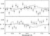 |
Fig. 8 Scaled flux ratios compared to the time-average spectrum (Eqs. (2), (3)) for RGS. Upper panel: data and model for spectrum 5; Lower panel: same for the combined spectra 1 and 2. The data have been rebinned by another factor of two to 0.116 Å for clarity of display. The models are for component C only. For comparison with other figures, the band that is plotted corresponds to 0.69–0.83 keV. |
As for the pn, variations in components A and B are below the detectability limit so are not considered further. For component C, the 15–18 Å band is most promising for detecting changes (Fig. 8). Our model predicts the strongest contrast between spectra 1 and 2 on one side, which have almost the same transmission, and spectrum 5 that corresponds to the peak of the soft X-ray emission.
Two prominent features contribute to the difference shown in Fig. 8. First, the model predicts a strong change in a broad band between 16.5–17.5 Å. This is the same blend as the predicted blend in the pn data around 0.73 keV (Fig. 6). The main contributions are from to M-shell transitions of Fe ix–Fe xiii, cf. Table 3, and the O vii edge. Averaged over the 16.5–17.5 Å band, the model predicts an increase of R by +0.043 from observations 1 and 2 to observation 5. The data show a decrease instead of −0.028 ± 0.011. Thus, at the 6.5σ confidence limit we can exclude an instantaneous response for component C.
The second feature is the Fe xvii resonance absorption line (rest-wavelength 15.01 Å, observed at 15.5 Å due to the cosmological redshift). Averaged over two adjacent bins, the model for component C predicts a decrease of −0.060 from observations 1 and 2 to observation 5, while the data shows a slight increase of +0.05 ± 0.03. A part of this increase can be explained by contamination by component D, which also produces Fe xvii. Component D alone produces an increase of +0.024. Because the contributions from components C and D to the total Fe xvii column density are 59 and 41%, respectively (cf. Table 4 in Detmers et al. 2011), the combined predicted net decrease in the Fe xvii line is −0.026. This is off by 2.5σ from the observed value. Thus, the Fe xvii line is also not in good agreement with an instantaneous response.
For component D the largest changes are expected between spectrum 1 and 5, for the O viii Lyα line at 19.6 Å. Averaged over two bins, the observed increase of 0.02 ± 0.05 agrees with the prediction of +0.04, but of course also with the hypothesis of no changes.
Finally, for component E there is a group of features in the 11.3–12.8 Å band where the model predicts a significant change, from a value of −0.015 for spectrum 4 to an average of +0.007 for observations 6, 8, and 10. This increase by +0.022 is significantly higher (at the 2.5σ level) than the observed difference of −0.003 ± 0.010. Alternatively, fitting a linear function to the observed R-values for all ten observations to the predicted values yields a slope of +0.18 ± 0.40, 2σ off from the expected value of 1 for an immediate response. This strengthens our conclusion from the pn data that also component E does not show much evidence of an instantaneous response.
In the next section we investigate whether the observations agree with a lack of response or with a delayed response. For this, we need to solve the time-dependent ionisation balance equations.
5. Time-dependent photoionisation
5.1. Introduction
The time evolution of the ion concentrations in the outflow depends on the gas density. For high density, the gas responds fast to changes in the ionising flux and restores ionisation equilibrium at the new flux level. For low density, collisions between free electrons and ions are rare, and because of that it takes a long time to restore equilibrium. When the photoionising flux varies faster than this response time, the plasma may be continuously out of equilibrium and it is at best in equilibrium with the long-term average flux, on time scales longer than the response time of the plasma. See Krolik & Kriss (1995, Sect. 6) for a more extensive discussion of these effects.
For strong enhancements of the flux, the ionisation may proceed faster than recombination (see Fig. 5 of Nicastro et al. 1999, for a good example of this), but when the flux does not vary by orders of magnitude, as in the case of Mrk 509, the ionisation and recombination time scales are of the same order of magnitude.
In this section we present how we model the time-dependent ionisation following the method of Nicastro et al. (1999). We first determine the history of the ionising spectral energy distribution (SED) for our observations. Starting with the first Swift observation, for which we assume ionisation equilibrium, we calculate for each outflow component the time evolution of the ion concentrations, for a grid of values for the gas density. We then calculate the corresponding X-ray transmission for the different components, and compare those to the observed spectra. The density for each component (or a lower- or upper limit) is then determined from the best match of a model spectrum to the observed spectrum.
5.2. Time-dependent SEDs
As in Sect. 4.1, we use the detailed spectral fits of the ten XMM-Newton observations from Mehdipour et al. (2011). They model the continuum with four components:
-
1.
disc blackbody (DBB, SPEX model dbb), representing thedirect emission from the accretion disc. Free parameters are theemitting area ADBB and the temperature TDBB;
-
2.
a soft X-ray excess (SE, SPEX model comt), representing Comptonised emission from the disc in a warm plasma. Free parameters are the seed temperature of the photons (taken to be equal to TDBB), the plasma temperature Te, optical depth τ, and normalisation Ncomt;
-
3.
power law (PL, SPEX model pow), with free parameters the photon index Γ and the normalisation NPL;
-
4.
Fe-K line (Fe, SPEX model gaus), approximated by a Gaussian and characterised by its energy EFe, normalisation NFe, and Gaussian width σ.
We apply a high-energy cut-off to the spectrum, based on the INTEGRAL data modelling, as shown in Kaastra et al. (2011a, Fig. 3). The cut-off is represented by a multiplicative factor to the power-law component, and the shape of the cut-off is kept constant in time, because more details are lacking.
The best-fit parameters for the DBB, SE, and PL components are given in Mehdipour et al. (2011, Table 6). The parameters for the iron line are not given in that paper, but the effects of the iron line on the present analysis are weak, because its ionising flux is only ~0.5 and 0.2% of the ionising flux of the power-law component and the total ionising flux, respectively. For simplicity, we assume that its flux is constant at the average value for the ten XMM-Newton observations, 0.76 ph m-2 s-1, corresponding to 2.07 × 1035 W in the source rest frame. Our continuum model is therefore described by seven free parameters that vary as a function of time.
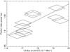 |
Fig. 9 Correlation between the photon index of the PL component with the UV flux for the ten XMM-Newton observations. The corners of the diamonds correspond to the nominal statistical uncertainty on both quantities. |
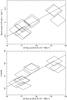 |
Fig. 10 Correlation between the normalisation Ncomt and optical depth τ of the soft excess (SE) component with the UV flux for the ten XMM-Newton observations. The corners of the diamonds correspond to the nominal statistical uncertainty on both quantities. |
Because the ionisation state of the gas also depends on the history of the ionising flux before the start of the XMM-Newton observations, we also need to characterise that part of the light curve. For that purpose we have obtained Swift observations as described by Kaastra et al. (2011a) and elaborated by Mehdipour et al. (2011). While for the ten XMM-Newton observations we had high signal-to-noise pn spectra and OM observations in all filters to constrain the SED, for the Swift observations, which had short exposure times, we have in most cases only UV fluxes for the UVM2 filter and broadband X-ray fluxes at 0.3 and 4 keV with a typical uncertainty of 0.05–0.10 dex (see Figs. 2 and 8 of Mehdipour et al. 2011).
These three fluxes (UV, 0.3 and 4 keV) per Swift observation are in principle insufficient for deriving the seven continuum parameters for the SED. However, there are tight correlations between these parameters, and therefore we can make a good proxy for the SED based on the UVM2 and the 4 keV fluxes alone, as we show below. We use the higher signal-to-noise and more detailed XMM-Newton observations to derive these correlations. For the Swift observations without the UVM2 filter, we estimate the UV flux from the other filters as described by Mehdipour et al. (2011).
For the power-law component, the photon index Γ correlates remarkably well with the UV flux (Fig. 9). The PL is then completely determined from the UV flux and the 4 keV X-ray flux, which has no contribution from the other softer continuum components.
For the soft excess component, the plasma temperature as given by Mehdipour et al. (2011) shows little variation, and thus we keep it constant at 0.20 keV. The normalisation Ncomt and optical depth τ of this component can be approximated as a linear function of the UV flux (Fig. 10), and as stated before, the temperature of the seed photons is tied to the disc blackbody.
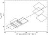 |
Fig. 11 Correlation between the temperature of the DBB component and the UV flux for the ten XMM-Newton observations. The corners of the diamonds correspond to the nominal statistical uncertainty on both quantities. |
Lower limits to the distance of the absorption components for different energy bands and instruments, at the 90% and 99% confidence levels.
Finally, for the disc blackbody component, there is a correlation between its temperature and the UV flux (Fig. 11). We kept its normalisation constant to 3.34 × 1025 m2, the mean value for the ten observations, and within the error bars, consistent with the reported values (Mehdipour et al. 2011, Table 6).
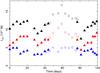 |
Fig. 12 Ionising luminosity (1–1000 Ryd) for the power-law component (blue), Comptonised component (red), and total spectrum (black). Filled triangles: based on Swift data; open circles: XMM-Newton observations. |
Using these correlations and the UVM2 and 4 keV flux, we constructed the time-dependent SEDs for our full 100 day campaign. Obviously, for the XMM-Newton observations we took the SEDs directly from Mehdipour et al. (2011) and we reported them in Sect. 4.1. A comparison of the ionising fluxes determined directly from the XMM-Newton data with the ionising fluxes determined through the above correlations shows a scatter of ~10%.
We show the ionising fluxes of the main components (PL and SE) in Fig. 12. It is seen that the luminosity before and after the XMM-Newton observations is lower than during these XMM-Newton observations. Most of the variability is caused by the soft excess component, although the power-law component also varies. The ionising luminosities of the disc-blackbody and iron line are much lower than the luminosities of the PL and SE components.
5.3. Solution of the time-dependent rates
The time dependence of the relative density ni of an ion i of a given species is given by 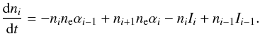 (4)Here ne is the electron density, and αi is the recombination rate from stage i + 1 to stage i and is in general a function of the temperature T. The ionisation rate from stage i to i + 1 is indicated by Ii. Obviously, in Eq. (4) ionisations from bare nuclei and recombinations onto neutral atoms should be excluded as they are non-existent.
Equation (4) forms a set of coupled ordinary differential equations. We solve these numerically by using a Runge-Kutta method with adaptive stepsize control, subroutine odeint from Press et al. (1992). Following Nicastro et al. (1999), we adopt a constant electron density ne as a function of time.
The recombination and ionisation rates are interpolated linearly between the values for the 29 different Swift and XMM-Newton observations. We also tried quadratic or spline interpolation, but that sometimes leads to unwanted overshooting, in particular near the start and the end of the XMM-observations where a few Swift observations are close in time to those by XMM-Newton. Moreover, such higher order schemes would hide the intrinsic uncertainties caused by the lack of data between the 29 observations.
The recombination and ionisation rates for the 29 epochs were obtained as follows. For each epoch and ionisation component, we calculated the equilibrium ion concentrations using Cloudy (Ferland et al. 1998) version C08.00, with Lodders et al. (2009) abundances. These equilibrium concentrations were calculated using the appropriate SED (see previous subsection). Furthermore, the ionisation parameters ξ were scaled down relative to the values obtained from the average XMM-Newton spectrum (Detmers et al. 2011), proportionally to the ionising 1–1000 Ryd luminosity L. For a prompt response of the gas to changes in flux or SED shape, this is the appropriate scaling, assuming that the gas density n and distance to the ionising source r remain constant in time (ξ = L/nr2). Using this same Cloudy run, we used the “punch ionization rates” option of Cloudy to obtain the corresponding ionisation and recombination rates. Since Cloudy takes multiple ionisation after inner-shell ionisation into account, the total ionisation rate obtained from the punch option does not return an equilibrium situation when inserted into our simplified Eq. (4), which ignores multiple ionisations. To correct for this we have scaled the ionisation rates Ii in our code so that equilibrium is forced (dni/dt = 0 in Eq. (4)) using the concentrations ni provided by Cloudy.
We did these calculations for a grid of distances r to the ionising source and for each of the outflow components separately. We assumed equilibrium for the first Swift spectrum as our initial condition.
5.4. Results
5.4.1. An illustrative example
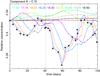 |
Fig. 13 Time evolution of the C iv concentration of component A, relative to the total carbon concentration. Stars: a model with instantaneous response to continuum variations. Coloured lines: predictions for absorbing material at different distances as indicated by the number near the top of the plot; these numbers represent the log of the distance in m. The XMM-Newton observations were taken between the two vertical dotted lines. |
We start here with C iv, an ion that mainly produces UV absorption but displays a number of interesting features in the time-dependent ion concentration. Figure 13 shows the predicted evolution of the ion concentration as a function of time for the dominant C iv contributor, component A.
For an instantaneous response, the relative C iv concentration varies between 0.23 and 0.34 in accordance with the continuum variability. For distances up to 1017.75 m, there is not much difference with the instantaneous response. For distances of 1018 and 1018.25 m, the response becomes delayed by about three and ten days, respectively. These delays are related to the lower densities and therefore longer recombination time scales corresponding to the longer distances (for constant L/ξ = nr2).
For greater distances, for instance 1018.50 m, the delay becomes a month but also the amplitude of the variations starts to decrease rapidly. The plasma is no longer able to respond to the fastest fluctuations of the ionising continuum. For even greater distances (>1018.75 m), the delay becomes longer than the duration of six week of the Swift monitoring before the start of the XMM-Newton observations, and the amplitude becomes significantly smaller. Here our model predictions become quite uncertain, as we lack sufficient information on the flux history of the years before the start of our campaign. There are only some sparse individual measurements available.
5.4.2. Time evolution for the most prominent ions
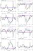 |
Fig. 14 Time evolution of the concentrations of several ions in components C and D. Further explanation see Fig. 13. |
In Fig. 14 we show the time evolution of the most important ions for our variability study (see Table 3). Starting with oxygen, we see that the strong soft X-ray flux enhancement near the centre of the XMM-Newton observations has a strong ionising effect: both the O vii and O viii concentrations decrease for gas at distances <1017.25 m; for longer distances, the history on longer time scales becomes more important.
Comparing Fe x with O vii, it is seen that iron responds faster to continuum changes than oxygen: a similar delay is found for iron at three times greater distances (compare the curves for O vii and Fe x at 1017.00 and 1017.50 m, respectively). For the iron M-shell ions Fe x – Fe xiii the lower ionisations stages show a decrease in column density while the higher ionisation stages show an increase near the centre of the XMM-Newton observations.
Finally, the two panels for Fe xvii for components C and D show that the response not only strongly depends on the distance to the central source, but also on the ionisation parameter: component D has a six times higher ionisation parameter than component C, and it responds in a less pronounced fashion.
5.4.3. Changes in the transmission
With the calculated time-dependent column densities, we next predict the changes in the transmission for each component as a function of distance. We compare the calculated transmission for individual observations to the calculated time-averaged transmission for all ten observations, similar to the spectral comparisons shown in Fig. 6. This average is different for each adopted distance, cf. the different curves in Fig. 14.
In Sect. 4 we found no evidence of an instantaneous response for any of the components where our sensitivity was sufficient to detect it. Here we follow a more general approach. For each ionisation component and for a grid of distances, we determine the formal agreement of the predicted ratio Rpred with the observed Robs by calculating χ2-values in given energy or wavelength bands. We summarise our findings in Table 6. In all cases, the best agreement was obtained for the assumption of no response (the low-density limit), so our data provide lower limits to the distances of the absorption components. The table also lists the χ2-value and degrees of freedom for the low-density limit (no response). The offsets in χ2-values from the degrees of freedom are caused by the slight mismatch of our continuum model for some of the observations (see Sect. 4.2) but these do not affect our distance estimates because they depend on the relative increases in χ2 and not on the absolute values.
For component C, the comparison of the pn results for the 0.5–1.5 and 0.62–0.78 keV band shows that the highest sensitivity is reached by using the broader band. This is in line with Fig. 6, which shows that, apart from the main peak at 0.72 keV, there is also a weaker contribution from the broader 1.0–1.5 keV band. The RGS data in the 16.5–17.5 Å band yield a distance limit that is almost equal to the limit obtained from the pn data. The narrower band around Fe xvii (15.4–15.6 Å) also yields lower limits, but these are less restrictive than the limits from the broader band.
For component D, the pn data cannot distinguish the different cases well so we only get a lower limit from the O viii Lyα line as measured by RGS. For component E the pn spectrum provides the best limit.
Combining our results for component C from pn and RGS, and taking the most restrictive limits for components D (RGS) and E (pn), Table 7 summarises the 90% confidence lower limits to the distance and density of components C–E.
6. Long-term variability
In the previous section we have shown that there are no indications of a change in the absorption components C–E during our intensive XMM-Newton monitoring period of 36 days. Here we investigate the longer-term variability. To this aim we have investigated the five archival XMM-Newton observations taken between 2000–2006. Similarly to the analysis of the data obtained during our campaign, we divided the fluxed pn spectra for all these observations by the fluxed pn spectrum of the combined 2009 observations. As a first step, we simply fit the ratios of the fluxed spectra to a power law plus three Gaussians in the 0.5–1.5 band. For the Gaussians we keep the centroids and widths fixed to the values given in Table 2, representing the expected differences due to changes in the ionising luminosity. We plot these ratios, with the local power-law model divided out, in Fig. 15. We list the best-fit amplitudes for the Gaussians in Table 8.
It is clear from Fig. 15 and Table 8 that there are no significant differences in transmission between the 2005 and 2009 spectra. There may be a hint for a small difference for component D in the 2006 spectrum, but it is not very strong.
The strongest differences are visible in the 2000 and 2001 spectra. For that reason, we have done a more sophisticated analysis of the continuum spectrum for those two observations. We also extracted the XMM-Newton OM fluxes for those observations and did spectral fits to both spectra using exactly the same model as Mehdipour et al. (2011); see also Sect. 5.2 for a description of the spectral model they used.
According to this continuum modelling, the ionising luminosity during the 2000 and 2001 observations is lower by −0.45 and −0.23 dex. We calculated the corresponding difference in transmission using the method described in Sect. 4 for the 2009 spectra. We show the results as a comparison of the observed ratio Robs to the predicted ratio Rpred (cf. Eqs. (2), (3)) in Fig. 16.
The broad dips that are visible in the 2000 and 2001 spectral ratios shown in Fig. 15 between 0.7–1.2 keV have almost disappeared. This is due to the more realistic broad-band optical to X-ray modelling of the continua in the present case, compared with the local 0.5–1.5 keV power-law approximation used in Fig. 15. Furthermore, the spectra are not sensitive enough to detect changes for component C. For component D, both spectra show a narrow dip in the data around 0.8 keV. When fitted with a Gaussian with centroid and width frozen to the values for component D taken from Table 2, we find best-fit amplitudes N of −0.014 ± 0.006 and −0.020 ± 0.004 for the 2000 and 2001 spectra, respectively. These values correspond to a nominal decrease in ξ of −0.23 ± 0.10 and −0.33 ± 0.07 dex. Finally, it is evident that the large changes that are predicted to occur for component E are not present. Thus, component E appears to be stable in ionisation parameter over ten years. This can only be explained by a low density, such that either there are no changes at all over ten years, or that the average ionising fluxes over the few months before each of the 2000, 2001 and 2009 observations were similar by coincidence.
Comparison of the 2000 and 2001 spectra shows that the quality of the data does not allow us to establish whether there are differences in the transmission between these spectra.
7. Discussion and conclusions
In this paper we have constrained the distance of the dominant X-ray outflow components in Mrk 509. This has been a challenging task, given the complexity of the problem and the refined analysis that is necessary.
The key to achieving these results was the deep 600 ks time-averaged RGS spectrum that allowed us to derive the ionisation structure of the outflow as seen through X-ray absorption lines (Detmers et al. 2011). The discrete components found in that work allowed us to make predictions for the time-dependent transmission of the outflow for different distances to the central source, and the distance limits were obtained by comparing those predictions with the observed spectra.
Another necessary ingredient in our analysis was the accurate broad-band spectral modelling from the optical to the hard X-ray band (Mehdipour et al. 2011). This was not only important for deriving the shape of the ionising continuum, but also for obtaining the underlying continuum spectrum for each observation in the energy band around 1 keV where most of the changes in transmission from the outflow are expected to occur.
Combined lower limits to the distance and density of the absorption components at the 90% confidence level.
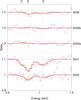 |
Fig. 15 Observed ratios of the fluxed pn spectra of Mrk 509 taken between 2000 and 2006 to the stacked spectrum taken in 2009, in the 0.5–1.5 keV band. As described in the text, a local power-law approximation to the continuum ratios has been taken out. Dotted vertical lines indicate the centroids for three Gaussian components (Table 2) that represent the expected changes of the transmission associated to the ionising flux differences. The solid curves indicate the best-fit sum of three Gaussians to the residuals. For clarity of display, the curves for each spectrum have been shifted along the y-axis by multiples of 0.1. |
We have used here the continuum models as derived by Mehdipour et al. (2011). These were based on the measured OM and pn spectra, but also on the scaled, non-simultaneous FUSE spectra described in that paper. This gives an excellent empirical description of the spectra (see also below). Relieving the constraints from FUSE yields somewhat different parameters for the continuum components from the ones used here (see Petrucci et al., in prep.), but their effects on the present results are minor.
Our analysis has shown that in the pn-band the continuum model spectra are accurate down to the 1% level (Sect. 4.2) and that narrow-band time variations can be detected with the pn down to the 0.5% level (Sect. 2.1.1). For our Mrk 509 data, an instantaneous response to the ionising continuum would predict changes up to 2% at certain energies for some of the ionisation components (for example between spectra 1 and 4, Fig. 6). Given the detection limits that we mentioned, this is certainly a detectable signal. For the somewhat lower ionised components with the dominant absorption troughs below ~1 keV, RGS gives useful constraints through the same blends as visible with pn, but also through some strong individual absorption lines (Fe xvii, O viii).
However, our data show no evidence of an instantaneous response to the continuum variations, as outlined in Sects. 4.2 and 4.3. Therefore we exclude the high-density limit for the gas, implying that the absorber must be located farther away from the central black hole. Our monitoring with Swift before the onset of the actual XMM-Newton monitoring (Kaastra et al. 2011a; Mehdipour et al. 2011) has been very important. It allowed us to develop and use a realistic time-dependent photoionisation model that predicts the change in transmission for a broad range of recombination time scales, hence distances to the ionising source.
In our time-dependent calculations, we assumed equilibrium for the first Swift observation as an initial condition. Because the first XMM-Newton observation starts six weeks later, most uncertainties due to this initial condition will be washed out for time scales shorter than this. On longer time scales this is not the case. We note, however, that the flux during our XMM-Newton observations was slighty higher than the long-term average flux, while the first Swift observations was perhaps closer to this long-term average.
Parameters for the model of a power law plus three Gaussians fitted to the pn spectra of Mrk 509 taken between 2000–2006, divided by the 2009 spectrum as described in the text.
Again comparing our predictions with the data, we have put tight lower limits to the distance and density of components C–E. Comparing our spectra taken in 2009 with archival data, in particular those taken in a relatively low flux state in 2000 and 2001, showed changes for component D on time scales of 8.5 years. This is 50 times the duration of our monitoring campaign, so it yields a 50 times lower limit to the density compared to the number given in Table 7, of 2.1 × 10⁸ m-3, with a corresponding upper limit to the distance of 33 pc.
In the long term, we see no detectable changes for components C and E. This does not imply automatically that no changes have occurred for those components, but we lack adequate monitoring before the 2000 and 2001 observations. Given the lack of short-term variability for components C–E, the ionisation equilibrium depends on the time-averaged spectrum for periods of months to years.
Because Mrk 509 can show ionising flux variations up to about 40%, this means in practice that for any spectrum taken, the ionising flux used to calculate the ionisation balance for the analysis of the absorber is also uncertain by that order of magnitude. In our case, the average flux during our XMM-Newton campaign may have been somewhat enhanced, perhaps by 15–20%, compared to the long-term average, due to the outburst that peaked around the epoch of spectra 4 and 5. This would, in retrospect, justify some minor corrections to the precise values of ξ that we derived from the time-average RGS spectrum (Detmers et al. 2011), but they do not alter the general picture.
It is possible to derive upper limits to the distance using a rather simple argument. Our lower limits to the distance r imply an upper limit to the density n through n = L/ξr2. Because the typical thickness of the absorbing layer a is related to the measured column density NH = na, we derive a lower limit to the relative thickness a/r. Reversing the argument, because a/r must be smaller than unity, we get an upper limit to the distance. For our components C–E these are 9 kpc, 1.3 kpc, and 21 pc, respectively. The limit for component C is not very useful, and for component D we have already found an upper limit of 33 pc from the long-term variability, but the limit for component E is interesting.
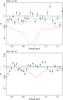 |
Fig. 16 Data points with error bars: observed ratios of the spectra taken in 2000 (upper panel) and 2001 (lower panel) to the average spectrum taken in 2009 in the representation of Eq. (2). We use here realistic continuum models (see text) rather than simplified local power laws as used in Fig. 15 to take out the changes of the continuum. Solid green lines: predicted ratio in the representation of Eq. (3) for ionisation component C; dashed blue lines: same for component D; dotted red lines: same for component E; thick magenta line: components A–E combined. The predictions for components A and B are close to zero and not shown here separately. |
There is a caveat here, however. In this paper, we have used the five ionisation components A–E derived from a direct fit to the total measured column densities. Detmers et al. (2011) also fitted the RGS spectrum directly using the xabs model of SPEX. The components found that way are, within their statistical uncertainties, compatible with what we use here, but for component E there are larger uncertainties. We have used log ξ = 3.60 ± 0.27, while the direct fit with the xabs model yielded log ξ = 3.26 ± 0.06. As discussed by Detmers et al. (2011) this is the same component; the differences arise mainly because component E is dominated in the RGS band by Fe xxi and Fe xxii. Making the ionisation parameter larger but also increasing the total hydrogen column yields almost the same ionic column densities for these ions.
We re-ran all our procedures but with the ionisation parameters and column densities replaced by those based on a direct xabs fit (Table 5 in Detmers et al. 2011). In particular for component E the upper limit to the distance from the constraint a/r < 1 increases significantly, from 21 pc to 400 pc. For the other components the differences are not very important.
Using the Chandra LETGS data of our campaign, Ebrero et al. (2011) also derived upper limits of 300 and 50 pc for the components C and the blend of D and E, respectively. These limits are consistent with our present findings, but Ebrero et al. (2011) had to make the additional assumptions that the solid angle of the outflow is ~π sr, and that the momentum of the outflow is close to the momentum of the scattered and absorbed radiation, cf. Blustin et al. (2005). Our present estimates are more direct.
Detmers et al. (2010) analysed the XMM-Newton spectra of Mrk 509 taken in 2005 and 2006. A simultaneous fit to the pn and RGS data of these spectra showed three ionisation components that correspond to our components B, C, and a blend of D and E. Components B and C did not show any significant variability between the observations. The fits of Detmers et al. (2010) indicate that the ionisation parameter for component D/E had decreased from 3.29 ± 0.04 in the first observation of 2005 to 3.01 ± 0.06 in the 2006 observation. From this change within 0.5 year an upper limit to the distance of 0.5 pc was derived. Such a value clearly contradicts our lower limit of about 5 pc for components D and E. With our present model, however, a change in 0.5 year would correspond to a distance of about 15 pc, much larger than 0.5 pc. The discrepancy can be traced down to the use of Fe xii to estimate the recombination time scale by Detmers et al. (2010). This ion has its peak concentration near the ionisation parameter for component D/E. It is therefore relatively insensitive to changes in the ionising flux. As a consequence, the formal recombination time scale (Eq. (4) in Detmers et al. 2010) becomes very large, leading to high density and short distance. Furthermore, the apparent change in transmission between 2005 and 2006 is possibly affected by some systematic effects and less significant than the formal 3.9σ significance quoted above. Factors contributing to a larger uncertainty are the lack of multi-pointing mode data for the RGS spectra in 2005 and 2006, the shorter exposure times leading to the detection of only three out of the five ionisation components, blending of ionisation components D and E, and global fitting with imperfect effective area instead of using ratios like in the present paper. The combined difference signal from components D and E between the first 2005 and the 2006 spectrum taken from Table 8 are, however, still consistent with a change at the 2.5σ significance level. We keep it open here whether this change is real or not, but if it is real, the upper limit of ~15 pc, according to our improved calculations, is close to the limit of 21–400 pc obtained from the requirement that a/r < 1 for component E as derived earlier in this section.
The distance limits derived in this paper (Table 7) imply an origin in the NLR or torus region of Mrk 509, rather than in the accretion disc. The limits are fully compatible with the upper limit of 250 pc derived from UV variability of the fastest UV outflow component (Kriss et al. 2011). This does not exclude an accretion-disc wind component. Perhaps the highly ionised, fast (0.05c, Ponti et al. 2009), or ultra-fast (0.14–0.20c, Cappi et al. 2009; Tombesi et al. 2010) outflows found in archival high-energy spectra of Mrk 509, but not found in our present data, could be examples of such a disc outflow. We defer a comprehensive overview of the various absorption components, combining both the ultraviolet and X-ray data, to another paper (Ebrero et al., in prep.).
In summary, we derived distance limits for the main X-ray absorption components in Mrk 509. Component C has a distance of >70 pc, component D is between 5–33 pc, and component E has a distance >5 pc but less than 21–400 pc, depending upon modelling details.
Acknowledgments
This work is based on observations obtained with XMM-Newton, an ESA science mission with instruments and contributions directly funded by ESA Member States and the USA (NASA). It is also based on observations with INTEGRAL, an ESA project with
instrument and science data centre funded by ESA member states (especially the PI countries: Denmark, France, Germany, Italy, Switzerland, Spain), Czech Republic, and Poland and with the participation of Russia and the USA. This work made use of data supplied by the UK Swift Science Data Centre at the University if Leicester. SRON is supported financially by NWO, the Netherlands Organization for Scientific Research. J.S. Kaastra thanks the PI of Swift, Neil Gehrels, for approving the TOO observations. M. Mehdipour acknowledges the support of a Ph.D. studentship awarded by the UK Science & Technology Facilities Council (STFC). N. Arav and G. Kriss gratefully acknowledge support from NASA/XMM-Newton Guest Investigator grant NNX09AR01G. Support for HST Program number 12022 was provided by NASA through grants from the Space Telescope Science Institute, which is operated by the Association of Universities for Research in Astronomy, Inc., under NASA contract NAS5-26555. E. Behar was supported by a grant from the ISF. S. Bianchi, M. Cappi, and G. Ponti acknowledge financial support from contract ASI-INAF n. I/088/06/0. P.-O. Petrucci acknowledges financial support from CNES and the French GDR PCHE. G. Ponti acknowledges support via an EU Marie Curie Intra-European Fellowship under contract No. FP7-PEOPLE-2009-IEF-254279. K. Steenbrugge acknowledges the support of Comité Mixto ESO – Gobierno de Chile.
References
- Anderson, K. S., & Kraft, R. P. 1969, ApJ, 158, 859 [NASA ADS] [CrossRef] [Google Scholar]
- Blustin, A. J., Page, M. J., Fuerst, S. V., Branduardi-Raymont, G., & Ashton, C. E. 2005, A&A, 431, 111 [NASA ADS] [CrossRef] [EDP Sciences] [Google Scholar]
- Cappi, M., Tombesi, F., Bianchi, S., et al. 2009, A&A, 504, 401 [NASA ADS] [CrossRef] [EDP Sciences] [Google Scholar]
- Crenshaw, D. M., Kraemer, S. B., Boggess, A., et al. 1999, ApJ, 516, 750 [NASA ADS] [CrossRef] [Google Scholar]
- Crenshaw, D. M., Kraemer, S. B., & George, I. M. 2003, ARA&A, 41, 117 [NASA ADS] [CrossRef] [Google Scholar]
- den Herder, J. W., Brinkman, A. C., Kahn, S. M., et al. 2001, A&A, 365, L7 [NASA ADS] [CrossRef] [EDP Sciences] [Google Scholar]
- Detmers, R. G., Kaastra, J. S., Costantini, E., et al. 2010, A&A, 516, A61 [NASA ADS] [CrossRef] [EDP Sciences] [Google Scholar]
- Detmers, R. G., Kaastra, J. S., Steenbrugge, K. C., et al. 2011, A&A, 534, A38 (Paper III) [NASA ADS] [CrossRef] [EDP Sciences] [Google Scholar]
- Ebrero, J., Kriss, G. A., Kaastra, J. S., et al. 2011, A&A, 534, A40 (Paper V) [NASA ADS] [CrossRef] [EDP Sciences] [Google Scholar]
- Ferland, G. J., Korista, K. T., Verner, D. A., et al. 1998, PASP, 110, 761 [Google Scholar]
- Gabel, J. R., Kraemer, S. B., Crenshaw, D. M., et al. 2005, ApJ, 631, 741 [NASA ADS] [CrossRef] [Google Scholar]
- Halpern, J. P. 1984, ApJ, 281, 90 [NASA ADS] [CrossRef] [Google Scholar]
- Kaastra, J. S., Mewe, R., & Nieuwenhuijzen, H. 1996, in UV and X-ray Spectroscopy of Astrophysical and Laboratory Plasmas, ed. K. Yamashita, & T. Watanabe, 411 [Google Scholar]
- Kaastra, J. S., Mewe, R., Liedahl, D. A., Komossa, S., & Brinkman, A. C. 2000, A&A, 354, L83 [NASA ADS] [Google Scholar]
- Kaastra, J. S., Raassen, A. J. J., Mewe, R., et al. 2004, A&A, 428, 57 [NASA ADS] [CrossRef] [EDP Sciences] [Google Scholar]
- Kaastra, J. S., Petrucci, P.-O., Cappi, M., et al. 2011a, A&A, 534, A36 (Paper I) [NASA ADS] [CrossRef] [EDP Sciences] [Google Scholar]
- Kaastra, J. S., de Vries, C. P., Steenbrugge, K. C., et al. 2011b, A&A, 534, A37 (Paper II) [NASA ADS] [CrossRef] [EDP Sciences] [Google Scholar]
- Kraemer, S. B., Crenshaw, D. M., Gabel, J. R., et al. 2006, ApJS, 167, 161 [NASA ADS] [CrossRef] [Google Scholar]
- Kriss, G. A., Arav, N., Kaastra, J. S., et al. 2011, A&A, 534, A41 (Paper VI) [NASA ADS] [CrossRef] [EDP Sciences] [Google Scholar]
- Krolik, J. H., & Kriss, G. A. 1995, ApJ, 447, 512 [NASA ADS] [CrossRef] [Google Scholar]
- Lodders, K., Palme, H., & Gail, H. 2009, in Landolt-Börnstein – Group VI Astronomy and Astrophysics Numerical Data and Functional Relationships in Science and Technology, Vol. 4B: Solar System, ed. J. E. Trümper, 4.4., 44 [Google Scholar]
- Mehdipour, M., Branduardi-Raymont, G., Kaastra, J. S., et al. 2011, A&A, 534, A39 (Paper IV) [NASA ADS] [CrossRef] [EDP Sciences] [Google Scholar]
- Miller, J. M., Raymond, J., Reynolds, C. S., et al. 2008, ApJ, 680, 1359 [NASA ADS] [CrossRef] [Google Scholar]
- Moe, M., Arav, N., Bautista, M. A., & Korista, K. T. 2009, ApJ, 706, 525 [NASA ADS] [CrossRef] [Google Scholar]
- Nicastro, F., Fiore, F., Perola, G. C., & Elvis, M. 1999, ApJ, 512, 184 [NASA ADS] [CrossRef] [Google Scholar]
- Phillips, M. M., Baldwin, J. A., Atwood, B., & Carswell, R. F. 1983, ApJ, 274, 558 [Google Scholar]
- Ponti, G., Cappi, M., Vignali, C., et al. 2009, MNRAS, 394, 1487 [NASA ADS] [CrossRef] [Google Scholar]
- Press, W. H., Teukolsky, S. A., Vetterling, W. T., & Flannery, B. P. 1992, Numerical recipes in FORTRAN. The art of scientific computing (Cambridge: University Press), 2nd edn. [Google Scholar]
- Strüder, L., Briel, U., Dennerl, K., et al. 2001, A&A, 365, L18 [NASA ADS] [CrossRef] [EDP Sciences] [Google Scholar]
- Tombesi, F., Cappi, M., Reeves, J. N., et al. 2010, A&A, 521, A57 [NASA ADS] [CrossRef] [EDP Sciences] [Google Scholar]
- Turner, M. J. L., Abbey, A., Arnaud, M., et al. 2001, A&A, 365, L27 [NASA ADS] [CrossRef] [EDP Sciences] [Google Scholar]
All Tables
Approximation with Gaussian components of the changes in transmission due to an increase of 0.1 dex in log ξ.
Strongest contributions to the dominant absorption troughs for components C, D, and E.
The 10log of the ionising (1–1000 Ryd) flux for the ten individual spectra 1–10 divided by the corresponding flux for the time-averaged spectrum, for each of the spectral components as modelled by Mehdipour et al. (2011).
Lower limits to the distance of the absorption components for different energy bands and instruments, at the 90% and 99% confidence levels.
Combined lower limits to the distance and density of the absorption components at the 90% confidence level.
Parameters for the model of a power law plus three Gaussians fitted to the pn spectra of Mrk 509 taken between 2000–2006, divided by the 2009 spectrum as described in the text.
All Figures
|
Fig. 1 Fluxed pn spectrum for the co-added 2009 spectrum of Mrk 509. The spectrum has been multiplied by E2 for clarity in the display. |
| In the text | |
|
Fig. 2 Ratio of the “fluxed” pn count spectrum to the fluxed photon spectrum of Mrk 509. |
| In the text | |
|
Fig. 3 1σ relative uncertainty on the individual ~60 ks RGS spectra of Mrk 509 per 0.058 Å bin. |
| In the text | |
|
Fig. 4 Transmission for the five ionisation components A–E at the resolution of the pn instrument (solid lines). Dotted lines: the same but for log ξ0.1 dex higher. Dashed lines: ratios of the transmission for the higher of the above ionisation states to the lower ionisation states. We use the same colour coding for each component. |
| In the text | |
|
Fig. 5 Ratio of the ten model spectra to the time-averaged model spectrum, based on the fits by Mehdipour et al. (2011). Only the underlying continua are taken into account, not the absorption components. The spectra as displayed are extrapolated outside the XMM-Newton range for illustrative purposes. |
| In the text | |
|
Fig. 6 Data points with error bars: observed ratios of the ten spectra (labelled 1–10) to the average spectrum in the representation of Eq. (2) (essentially the spectral ratios with the respective continua divided out and unity-subtracted). Solid green lines: predicted ratio in the representation of Eq. (3) for ionisation component C; dashed blue lines: same for component D; dotted red lines: same for component E; thick magenta line: components A–E combined. The predictions for components A and B are close to zero and not shown here separately. |
| In the text | |
|
Fig. 7 Example of continuum adjustment for spectra 4 (top panel) and 5 (bottom panel). Data points with error bars: observed ratio of spectra 4 and 5 to the average spectrum in the representation of Eq. (2), same as in Fig. 6. Solid black line: cubic polynomial fit to R over the 0.4–3.2 keV band as described in the text. Solid green line: predicted R in the representation of Eq. (3) for component C, but added here to the continuum approximation given by the black line; dashed blue line: same for component D; dotted red line: same for component E; thick magenta line: components A–E combined. |
| In the text | |
|
Fig. 8 Scaled flux ratios compared to the time-average spectrum (Eqs. (2), (3)) for RGS. Upper panel: data and model for spectrum 5; Lower panel: same for the combined spectra 1 and 2. The data have been rebinned by another factor of two to 0.116 Å for clarity of display. The models are for component C only. For comparison with other figures, the band that is plotted corresponds to 0.69–0.83 keV. |
| In the text | |
|
Fig. 9 Correlation between the photon index of the PL component with the UV flux for the ten XMM-Newton observations. The corners of the diamonds correspond to the nominal statistical uncertainty on both quantities. |
| In the text | |
|
Fig. 10 Correlation between the normalisation Ncomt and optical depth τ of the soft excess (SE) component with the UV flux for the ten XMM-Newton observations. The corners of the diamonds correspond to the nominal statistical uncertainty on both quantities. |
| In the text | |
|
Fig. 11 Correlation between the temperature of the DBB component and the UV flux for the ten XMM-Newton observations. The corners of the diamonds correspond to the nominal statistical uncertainty on both quantities. |
| In the text | |
|
Fig. 12 Ionising luminosity (1–1000 Ryd) for the power-law component (blue), Comptonised component (red), and total spectrum (black). Filled triangles: based on Swift data; open circles: XMM-Newton observations. |
| In the text | |
|
Fig. 13 Time evolution of the C iv concentration of component A, relative to the total carbon concentration. Stars: a model with instantaneous response to continuum variations. Coloured lines: predictions for absorbing material at different distances as indicated by the number near the top of the plot; these numbers represent the log of the distance in m. The XMM-Newton observations were taken between the two vertical dotted lines. |
| In the text | |
|
Fig. 14 Time evolution of the concentrations of several ions in components C and D. Further explanation see Fig. 13. |
| In the text | |
|
Fig. 15 Observed ratios of the fluxed pn spectra of Mrk 509 taken between 2000 and 2006 to the stacked spectrum taken in 2009, in the 0.5–1.5 keV band. As described in the text, a local power-law approximation to the continuum ratios has been taken out. Dotted vertical lines indicate the centroids for three Gaussian components (Table 2) that represent the expected changes of the transmission associated to the ionising flux differences. The solid curves indicate the best-fit sum of three Gaussians to the residuals. For clarity of display, the curves for each spectrum have been shifted along the y-axis by multiples of 0.1. |
| In the text | |
|
Fig. 16 Data points with error bars: observed ratios of the spectra taken in 2000 (upper panel) and 2001 (lower panel) to the average spectrum taken in 2009 in the representation of Eq. (2). We use here realistic continuum models (see text) rather than simplified local power laws as used in Fig. 15 to take out the changes of the continuum. Solid green lines: predicted ratio in the representation of Eq. (3) for ionisation component C; dashed blue lines: same for component D; dotted red lines: same for component E; thick magenta line: components A–E combined. The predictions for components A and B are close to zero and not shown here separately. |
| In the text | |
Current usage metrics show cumulative count of Article Views (full-text article views including HTML views, PDF and ePub downloads, according to the available data) and Abstracts Views on Vision4Press platform.
Data correspond to usage on the plateform after 2015. The current usage metrics is available 48-96 hours after online publication and is updated daily on week days.
Initial download of the metrics may take a while.