| Issue |
A&A
Volume 696, April 2025
|
|
|---|---|---|
| Article Number | A50 | |
| Number of page(s) | 10 | |
| Section | Extragalactic astronomy | |
| DOI | https://doi.org/10.1051/0004-6361/202451710 | |
| Published online | 02 April 2025 | |
Investigating the complex absorbers of Mrk 766 with XMM-Newton
1
SRON Netherlands Institute for Space Research, Niels Bohrweg 4, 2333 CA Leiden, The Netherlands
2
Anton Pannekoek Institute, University of Amsterdam, Postbus 94249 1090 GE Amsterdam, The Netherlands
3
School of Physics, HH Wills Physics Laboratory, University of Bristol, Tyndall Avenue, Bristol BS8 1TL, UK
4
MIT Kavli Institute for Astrophysics and Space Research, Massachusetts Institute of Technology, Cambridge, MA 02139, USA
5
Department of Astronomy and Astrophysics, University of Chicago, Chicago, IL 60637, USA
⋆ Corresponding author; This email address is being protected from spambots. You need JavaScript enabled to view it.
Received:
29
July
2024
Accepted:
13
January
2025
Abstract
Aims. We examine the high-energy resolution X-ray spectrum of the narrow-line Seyfert 1 galaxy Mrk 766 using four observations taken with XMM-Newton in 2005 to investigate the properties of the complex ionised absorber and/or emitter along the line of sight, as well as absorption by dust intrinsic to the source.
Methods. We used the high-energy resolution RGS spectrum to infer the properties of the intervening matter. We also used the spectrum obtained by EPIC-pn and the photometric measurements of OM to obtain the spectral energy distribution of the source, which is necessary for the photoionisation modelling of the ionised outflow.
Results. The warm absorber in Mrk 766 consists of two phases of photoionisation. In addition to these two warm absorber components with log ξ ∼ 2.15 and log ξ ∼ −0.58, we found evidence of absorption by a collisionally ionised component (T ∼ 51 eV). We discuss the implication of this additional component in the light of theoretical predictions. Moreover, we detected signs of absorption by a dusty medium with Ndust ∼ 7.29 × 1016 cm−2. Finally, the relatively weak emission features in the spectrum seem to be unrelated to the absorbers and probably originated by ionised plasma beyond the line of sight.
Key words: techniques: spectroscopic / galaxies: active / galaxies: individual: Mrk 766 / galaxies: Seyfert / X-rays: galaxies
© The Authors 2025
 Open Access article, published by EDP Sciences, under the terms of the Creative Commons Attribution License (https://creativecommons.org/licenses/by/4.0), which permits unrestricted use, distribution, and reproduction in any medium, provided the original work is properly cited.
This article is published in open access under the Subscribe to Open model. This email address is being protected from spambots. You need JavaScript enabled to view it. to support open access publication.
1. Introduction
It is standard for the spectra of Seyfert galaxies to show absorption features that are due to photoionised gas in our line of sight (Kaastra et al. 2000; Blustin et al. 2005; Costantini et al. 2007; Mehdipour et al. 2010). This outflowing gas is often referred to as warm absorbers (WAs) and is particularly common in Seyfert 1 galaxies (Reynolds & Fabian 1995; Laha et al. 2014, 2020). WAs imprint narrow absorption lines and edges on the X-ray spectrum of active galactic nuclei (AGN). In most cases, more than one phase of a WA is present in the AGN, where each phase constitutes a region in the gas that is outflowing with a specific ionisation parameter (ξ), column density (NH), and velocity (vout).
The AGN outflows are thought to provide a link between the co-evolution of supermassive black holes (SMBHs) and their host galaxies (Fabian 2012; King & Pounds 2015). They are suggested to regulate black hole growth (Crenshaw & Kraemer 2012) and to help establish the M − σ relation (Silk & Rees 1998; King & Pounds 2015). Moreover, they might also cause the quenching and/or enhancement of star formation, as they are able to enrich the gas in the galaxy and/or remove gas from the bulge and halo (Hopkins et al. 2005; Heckman & Best 2014).
The study of outflows is therefore important to establish this connection between SMBHs and their host galaxy. In particular, WAs provide us with insights into some of the innermost regions of AGN. However, there are still many open questions regarding the nature of WAs, including their origin, their geometrical structure, or their connection to the nucleus and the outer regions of the AGN. Some previous studies connected the origin of these absorbers to photoionised evaporation from the inner edge of the torus (Blustin et al. 2002; McKernan et al. 2007). Other works attempted to explain their geometry in the context of ionisation cones (Kinkhabwala et al. 2002), whereby it is possible for the WAs to appear in re-emission, depending on the inclination of the AGN (Kinkhabwala et al. 2002; Bianchi et al. 2006; Guainazzi & Bianchi 2007).
Nevertheless, photoionisation does not cause the ionised absorbing gas detected in the X-ray spectra of AGN alone. Various AGN have shown Fe absorption features that were associated with the presence of dust (Lee et al. 2001, 2013; Mehdipour & Costantini 2018; Psaradaki et al. 2024). Moreover, signatures of collisionally ionised absorbers (CIAs) were recently reported in NGC 4051 (Ogorzalek et al. 2022). Other sources presenting collisionally ionised absorbers include NGC 4151 (Wang et al. 2011), NGC 3393 (Maksym et al. 2019), and Mrk 573 (Paggi et al. 2012). The distance, and therefore, the origin, of these collisionally ionised absorbers is extremely difficult to derive because of the current instrumental resolution. This makes it hard to learn more about their energetics and geometrical properties.
There is also evidence that AGN, mostly Seyfert 1 s, can host narrow emission lines of C and O that are embedded in the absorption features produced by the WAs (Bianchi et al. 2006; Guainazzi & Bianchi 2007; Ebrero et al. 2010). Whether these lines are connected to the WAs is still an open question (Costantini 2010). However, the emission spectrum and its link to the WA could help us to obtain a better understanding of the processes that ionise these outflows and of the distances at which they originate. Guainazzi & Bianchi (2007) studied obscured AGN and reported emission in the form of radiative recombination continua (RRCs). This suggested that these features are likely created by photoionised gas. The authors demonstrated that resonant scattering significantly influenced the ionisation / excitation balance of the gas. Their results indicated that the column densities required for this emission matched those measured in WAs observed in unobscured AGN. However, the observed emission in AGN might originate from different regions within the system.
Depending on the type of AGN, the appearance of these emission lines may differ. The soft X-ray spectrum of highly obscured Seyfert 2 AGN is dominated by the emission from the H-like and He-like K transitions of light metals, which is likely created by photoionised gas that surrounds the AGN around the narrow-line region (NLR, Bianchi et al. 2006). This arises because the torus obscures all evidence of absorption that affects the continuum. However, the continuum emission of Seyfert 1 AGN is predominant because the torus does not obscure our line of sight, implying a favourable detection of absorption instead of emission (Costantini 2010). As the inclination of a source increases to somewhere between a Seyfert 1 and Seyfert 2, it is possible to some extent to distinguish these emission lines from the NLR from the different absorption features that affect the continuum.
We explore the complex absorbers in the soft X-ray spectrum of Mrk 766. This AGN is a nearby narrow-line Seyfert 1 galaxy (z ∼ 0.0129; Falco et al. 1999) with an SMBH of MBH ∼ 1.26 × 10⁶ M⊙ that is hosted in a barred spiral galaxy (Risaliti et al. 2010; Giacchè et al. 2014). It is one of the brightest sources of its class, with F2 − 10 keV ∼ 1.37 × 10⁻¹¹ erg cm−2 s −1 (this work), and has been observed by multiple X-ray observatories in different occasions. Previous studies have shown that the X-ray spectrum of Mrk 766 is variable and that it can be modelled with an absorbed power law and an accompanying ionised reflection (Turner et al. 2007). Moreover, the presence of WAs in its X-ray spectrum has long been established (George et al. 1998; McKernan et al. 2007; Laha et al. 2014; Winter et al. 2012), although previous XMM-Newton (Jansen et al. 2001) observations caused a debate of whether the complicated features in the soft X-ray spectrum of this source arise from a dusty warm absorber or from relativistic emission lines (Branduardi-Raymont et al. 2001; Lee et al. 2001; Sako et al. 2003; Mason et al. 2003).
Throughout this work, we adopt the following cosmological parameters: H0 = 70 kms−1 Mpc−1, Ωm = 0.3, and ΩΔ = 0.7. The analysis was carried out using the fitting package SPEX v3.08.00 (Kaastra et al. 1996; Kaastra 2017). To evaluate the goodness of fit, we used the C-statistic (Cash 1979; Kaastra 2017), and the reported uncertainties were calculated with a 1σ significance.
2. Observations and data processing
Mrk 766 was observed by XMM-Newton over a period of six orbits between May 23, 2005, and June 3, 2005. We chose to analyse four observations with the longest exposure times, comparable fluxes, and spectral shapes. We did not choose to use all six observations taken during this XMM-Newton campaign since we were interested in exploring the average properties of the AGN and its absorbers. Therefore, we decided to exclude observation 0304030101 because its flux is notably lower and the spectral shape is different (see Fig. 1). We also excluded observation 0304030701 because its exposure time is particularly shorter (about one-third of the average exposure time). The details for the chosen observations with their corresponding observation IDs, observation dates, and exposure times can be found in Table 1. We used data from the European Photon Imaging Camera pn instrument (EPIC-pn, Turner et al. 2001) in the 0.3 − 10 keV band, as well as data from the Reflection Grating Spectrometer (RGS; den Herder et al. 2001) in the 7 − 36 Å band and of the Optical Monitor (OM; Mason et al. 2001) filters B, U, UVW1, UVM2, and UVW2. We reduced the data using the Science Analysis System (SAS ver 20.0.0) and the HEASARC FTOOLS.
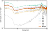 |
Fig. 1. Spectra of Mrk 766 taken with the XMM-Newton EPIC-pn instrument. The different observations taken during the 2005 campaign are shown in various colours. We show observations that were not included in the study in grey. We plot the merged spectrum of observations 301, 401, 501, and 601 in red. We refer to the observations by the last three digits of their observation IDs. |
XMM-Newton observations.
The EPIC-pn camera was operated in small-window mode. We verified with the SAS task epatplot that the observations were not affected by pile-up. Based on a 3σ clipping of the background count rate, the data from neither observation were significantly affected by flares. We extracted the spectrum from a circular region, centred around the source, of 30.6 arcsec. We used a region of the same radius to extract the background from a source-free area on the same chip. We created out-of-time event lists using the epchain task, and after filtering, we rescaled and removed them from the good-time intervals. Finally, we created the ancillary response file (ARF) and the redistribution matrix file (RMF) using the SAS commands arfgen and rmfgen, respectively.
The RGS instruments were operated in the Spectroscopy HER + SES mode, and the data were processed with the rgsproc task. We created good-time intervals with the tabgtigen command, and we generated light curves for RGS1 and RGS2 with eveselect and corrected them with rgslccorr for dead time and background scale, whilst performing background subtraction. Finally, we combined RGS1 and RGS2 with rgscombine.
The OM observations were obtained using the imaging and fast modes. These two modes were used together for most of the observations, where filters B, U, UVW1, UVM2, and UVW2 were applied, except for observation 0304030301, which only used the image mode with the grism filters. It was therefore not used for the purpose of this analysis. We used the SAS task omichain to filter the source lists. We combined the source list files with the coordinates for the source, which were cross-checked using the SIMBAD astronomical data base1, to obtain the raw count rates and the errors using the task om2pha.
We merged the different EPIC-pn, RGS, and OM observations using SAS, and created a combined set of response and spectrum files for each instrument. By doing so, we obtained a better signal-to-noise ratio to work with, which allowed us to determine the average characteristics of the absorbers. The individual observations and merged spectrum are shown in Fig. 1.
3. Spectral energy distribution
For the spectral energy distribution (SED), we used the merged EPIC-pn observations. As the OM photometric data did not change in the observations, we adopted the data from the 0304030401 observation (see Fig. 2). For the modelling, we followed the approach presented in Mehdipour et al. (2011), where the broad-band continuum was described by a seed black body from the accretion disk (DBB model in SPEX; Shakura & Sunyaev 1973). This radiation was then reprocessed by inverse-Compton scattering (Done et al. 2012; Kubota & Done 2018), creating a warm soft-X-ray emission component (COMT model in SPEX). The X-ray continuum was parametrised by a cut-off power law and a reflection component (REFL model in SPEX; Zycki et al. 1999).
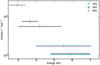 |
Fig. 2. Spectra of Mrk 766 taken with the XMM-Newton OM instrument. The different observations used for this study are shown in various colours. The OM filters from left to right are B, U, UVW1, UVM2, and UVW2. We refer to the observations by the last three digits of their observation IDs. |
We used the information obtained from the RGS fitting for the complex absorption components, which was needed to obtain the best broad-band fit. We fixed the Galactic cold and warm absorption and the dust absorbers in the host galaxy to the best-fit RGS values (Sect. 4, Table 3). At the end of this iterative process, the parameters of the warm absorbers detected by RGS were refined by the ionisation balance dictated by the broad-band SED. We added two photoionised absorbers to model the different phases of WAs and a collisionally ionised absorber to account for the additional absorption in the RGS data (Sect. 4), and we left the column density, ionisation parameter of the WAs, and temperature of the CIA free to vary, starting from the best-fit values. The free parameters were adjusted to the different resolution of EPIC-pn and any cross-calibration uncertainties that might still exist. Finally, for the OM data, we included an extinction component to account for the local extinction (E(B − V) = 0.017, Schlafly & Finkbeiner 2011), assuming RV = 3.1 and a Milky Way extinction law (Cardelli et al. 1989). A higher-extinction (E(B − V)∼0.38, Vasudevan et al. 2009) component at the redshift of the source was also added. In this case, we adopted an SMC extinction law (Gordon et al. 2003), which is thought to describe extinction in AGN better (Hopkins et al. 2004). The OM filter B was excluded from the analysis as the flux might still be contaminated by the stellar radiation in the host galaxy.
The broad-band continuum best fit was obtained with a disk black body with a temperature Tdbb = 10.4 ± 0.2 eV. This value was taken as the seed temperature for the Comptonisation component, with an optical depth τ = 10.4 ± 0.1 and a final temperature of T = 0.34 ± 0.02 keV. The high-energy cut-off of the power law, with a slope with Γ = 1.90 ± 0.02, remained unconstrained. We fixed the cut-off to 22 keV, keeping in mind that a large uncertainty exists on this value (Buisson et al. 2018). Finally, the fit required a modest reflection component, with an associated Fe Kα emission line. The inclination of the disk was set at 46° (Buisson et al. 2018), while the scale parameter in the REFL model was s < 3 × 10⁻³ (for reference, s = 1 would correspond to an isotropic source above the disk). Other parameters were kept at the default values because the SED modelling is limited by the lack of hard X-ray data. This makes it hard to determine the reflected spectrum of the source. An additional narrow Gaussian profile was required at E ∼ 6.7 keV.
The resulting SED is presented in Fig. 3. Its ionising luminosity, defined as the luminosity between 1 and 1000 Ryd, is Lion = 1.58 × 1044 erg s−1. This SED was then used with xabsinput in SPEX to calculate the ionisation balance that accompanies the XABS models in Sect. 4.
 |
Fig. 3. Model obtained from the SED fitting of the XMM-Newton EPIC-pn and OM merged observations. We show the best-fit model to the data in black. The curves in grey show the emission components that make up the model, which are from left to right DBB, COMT, POW, REFL, and GAUSS. The model of the absorbed spectrum is plotted in blue. |
4. RGS spectral analysis
For simplicity, and given the limited band of RGS, we modelled the continuum with a simple broken power-law model. In this model, we left the two slopes and the break energy free to vary. Given the prominent soft excess observed in this source, this phenomenological model mimics the curvature in the RGS band that is produced by the broader band Comptonisation model (Table 3).
4.1. Absorption features
Various types of absorption and emission signatures are present in the data. Figure 4 presents the merged RGS observations, where numerous spectral features can easily be distinguished by eye. Starting with the 16 − 23 Å region, absorption edges are apparent, which are consistent to be produced by Fe and O. This can be taken as a sign of dust being present in the line of sight (Lee et al. 2001, 2013; Mehdipour & Costantini 2018). Moreover, the apparent absorption features at the laboratory wavelengths of O I and O VII indicate the presence of both neutral and ionised gas intrinsic to the Milky Way (Steenbrugge et al. 2005; Costantini et al. 2007; Mehdipour & Costantini 2018). Furthermore, there is a plethora of other types of narrow absorption features that could be linked to the presence H and He-like transitions from C, N, O, and Ne, such as Ne X, Ne IX, or O VIII.
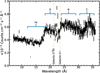 |
Fig. 4. Merged RGS data in black. We indicate the regions in which we expect ions of a certain element in the spectrum with horizontal lines. Features marked in yellow correspond to Galactic features, and blue indicates regions in which absorption / emission features by certain elements is expected. |
To account for neutral absorption in the Galaxy, we used the HOT component in SPEX with a temperature fixed at 1 × 10⁻⁶ keV. To portray the absorption caused by a warmer ISM gas, and therefore, to take the apparent O VII absorption feature at a wavelength of 21.6 Å into account, we added a second HOT. We allowed the column density of this component to be free, but limited its temperature within the range (5 − 7.5)×10−2 keV (Yao & Wang 2006).
To investigate the presence of WAs, we modelled their absorption features using the XABS component, which calculates the transmission of a slab of an ionised material, where all ionic column densities are linked through a photoionisation model (Steenbrugge et al. 2005). The provided SED dictates the ionisation balance, which sets the fractional abundance of different charge states of a particular element. We allowed the column density (NH), ionisation parameter (log ξ), outflowing velocity (vout), and covering factor (CV) of the absorbers to be free to vary. We initially fitted a single WA with log ξ = 0.88 ± 0.17, which provided us with a C-stat/d.o.f. of 2081/561. However, it became obvious from the residuals that additional absorption features were present in the lower and higher energy ranges of the RGS data. Therefore, we introduced two additional WAs with higher and lower log ξ values to cover the different energy regions. We found an ionised absorber with log ξ = 2.18 ± 0.05 and another at log ξ = 0.92 ± 0.02. These two components were found to partially cover the source, with a measured covering factor of 0.27 ± 0.01 and 0.70 ± 0.07. Finally, for the third lower-ionisation component (log ξ = −1.34 ± 0.25), the covering factor was consistent with unity. These additional two WA components improved the C-stat/d.o.f. from 2081/561 to 1564/553.
Although the introduction of the different WA phases improved the overall fit to the data, the residuals showed that additional absorption was still present that needed to be considered, particularly in the 16 − 20 Å region, as shown in the lower panel of Fig. 5. To account for the deep absorption jump at ∼17.7 Å, we considered absorption by dust at the redshift of the source, that is, within the system of Mrk 766. We chose to include a dust component (AMOL in SPEX) instead of another WA because of the potential Fe I absorption features in the spectra. These lines might be caused by either a cold absorber or by dust. The dust features in the RGS band mainly consist of absorption by Fe (17.71 Å) and O (22.83 Å). Therefore, we assumed a hematite composition (Fe2O3; Mehdipour et al. 2010). The addition of this component improved our fit from a C-stat/d.o.f. of 1564/553 to 1325/551, and it took into account the deep absorption jump at ∼17.7 Å. Moreover, it affected the ionisation values of the absorbers and shifted them to log ξ = 2.39 ± 0.05, log ξ = 0.96 ± 0.02, and log ξ = −0.80 ± 0.15. Figure 5 shows the improvement obtained by including a dust component in the overall fit to the data over this region.
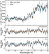 |
Fig. 5. Comparison between a model using a combination of three WAs and dust as opposed to WAs alone. Upper panel: Model implementing three WAs and dust (red) vs. WAs alone (blue). The latter case does not take into account the additional absorption in the 15 − 18 Å region, while the WAs and dust model does. The RGS data are shown in black. Middle panel: Residuals of the WA and dust model. Lower panel: Residuals of the WA model. |
However, the residuals of this model seemed to still show an excess in absorption in the entire 17 − 19 Å region. To mitigate this additional absorption, we tested the presence of a collisionally ionised absorber. In particular, we substituted the WA with log ξ ∼ 0.96 by a warm CIA (modelled with the SPEX component HOT), intrinsic to Mrk 766. We found that by adding this CIA, we improved our results in the 17 − 29 Å region. With a temperature T = 0.037 ± 0.002 keV, a column density of NH = (1.22 ± 0.04)×1022 cm−2, and a partial covering of CV = 0.53 ± 0.09, we found that this CIA provided a good fit to the data, where a model with WAs alone created a deeper absorption in this region. At a given temperature, the ionic column density distribution of a collisionally ionised gas peaks around a single ion, while for a photoionised gas, a range of ions is involved, leading to additional absorption when using XABS alone (van Peet et al. 2009). Statistically speaking, the inclusion of a collisionally ionised absorber improved our C-statistic, with a C-stat/d.o.f. = 3/551, as opposed to 1325/551 for a model that used WAs alone without CIAs. To ascertain that a model with a CIA was statistically better, we used the Akaike information criterion (AIC), by which if we have a collection of models for a given set of data, we can estimate the quality of each model relative to each other by investigating the relative amount of information lost by a model, where the less information lost, the better (Akaike 1974).
To decide between the models, we calculated the ΔAIC scores. The ΔAIC represents the difference between the best model obtained, which has the lowest Akaike criterion value (AICmin), and each of the other models (Burnham & Anderson 2002). The formula is given by ΔAIC = AICi–AICmin, where AICmin represents the lowest obtained AIC value, AICi stands for the other AIC values, and where all models must have the same degrees of freedom (Akaike 1974; Burnham & Anderson 2002). The higher the ΔAIC, the lower the probability that two models are equally acceptable for the data. When ΔAIC > 10, we can assume that AICi is not suitable when compared to AICmin. In this way, we concluded that a model with a CIA was more suitable because we obtained ΔAIC = 2 ≫ 10 (see Table 2). Figure 6 shows that a model without this additional collisionally ionised gas leads to additional absorption in the 17 − 19 Å region, and the addition of the CIA component clearly results in a better fit and better residuals. The models shown in Fig. 6 already include emission features (Sect. 4.2). Table 3 provides a summary of the best-fit parameter obtained for the absorption and emission components used in our model.
 |
Fig. 6. Comparison between a model using a combination of WAs and CIA as opposed to WAs alone. Upper panel: Transmission plot. Transmission is defined as the observed spectrum divided by the continuum. This plot compares the behaviour of the CIA (red) around the 13 − 20 Å region in comparison to a WA with log ξ ∼ 0.96 (blue). The transmissions obtained by the other WAs used in both models are shown in fainter red and blue. Upper middle panel: Difference between a model implementing WAs and CIA (red) as opposed to WAs alone (blue). “WAs and CIA” is used to indicate our best-fit model. “WAs” is meant to represent the model with three WAs and no CIA. It is apparent that the latter case creates additional absorption in the 17 − 18 Å region. The most prominent absorption features identified by our models are marked and labelled. Lower middle panel: Residuals of the CIA and WA model. Lower panel: Residuals of the WAs model. |
Akaike test parameters for the WAs and CIA fitting.
4.2. Emission lines
The best-fit absorption model showed some residuals in emission, especially at the energies corresponding to O and N, which may indicate the presence of an emitting plasma, as shown in the middle panel of Fig. 5. Therefore, we introduced a physically motivated emission model, PION, which is able to calculate the transmission and emission of a slab of photoionised plasma where the ionic column densities are related through a photoionisation model (Miller et al. 2015; Mehdipour et al. 2016). Since the origin of the emission embedded in the absorption features of AGN is not known in general, we investigated two different physical scenarios for emission to test the connection between WAs and emission.
The first scenario, Case 1, assumed that the emission is linked to the WAs and created in ionisation cones where re-emission occurs, resulting in narrow emission lines (Behar et al. 2003). The geometry of this scenario would involve the emission being created within the ionisation cone of the WA, which is in the line of sight of the observer. Moreover, the ionisation cone in this scenario would be near the dusty torus, meaning that the emission would not only be absorbed by the WA itself, but also by dust, as well as the ionised gas from the host galaxy and our own galaxy.
In the second scenario, Case 2, emission is created in the NLR. However, this time emission would not be absorbed by the galaxy material as it would originate from within some photoionised plasma situated far away from the ionising source. Therefore, it would not be absorbed by any dust or gas in the system.
We investigated these two different scenarios by creating models where we related the PION component differently with the other components in other to replicate the emission cases above. To evaluate the most appropriate emission case, we again used the Akaike criterion. We found that both scenarios were equally as likely to cause the emission in the spectra (Table 4). As discussed in Sect. 5, we adopted Case 2 while modelling the spectrum, which improved our C-stat/d.o.f. from 1243/551 for the model without emission to 1000/547 for the model accounting for emission. The addition of this emission also altered the parameters of some of the components in the model to those shown in Table 3.
Best-fit free parameters for the RGS data fitting.
Akaike test parameters for the PION fitting.
In Fig. 7 we show the transmission of all the best-fit absorbing components used in our model together with the data and the emission features that were predicted to be in the data when using PION in Case 2. Table 3 contains the parameters obtained for our best fit.
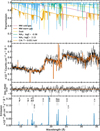 |
Fig. 7. Best fit model for the RGS data. Upper panel: Transmission plot. Transmission is defined as the observed spectrum divided by the continuum. The different absorbing components are explained in the legend. Middle upper panel: RGS data (black) with the best-fit model (red). Middle lower panel: Residuals from our best-fit model. Lower panel: Emission features predicted by PION in emission. The most prominent features are labelled. |
5. Discussion
We have presented an analysis of the OM, EPIC-pn, and RGS spectra for the narrow-line Seyfert 1 AGN Mrk 766. The high spectral resolution of the RGS gratings allowed us to find a plethora of absorption features that originated from the Galaxy and were intrinsic to Mrk 766.
The intrinsic absorption affecting the soft X-ray spectrum of Mrk 766 comprises two phases of WAs: dust, and a warm CIA. We noted that none of the WAs seem to be outflowing at high speeds, and their column densities and ionisation parameters are similar to the commonly observed ranges in Seyfert 1 AGN (McKernan et al. 2007; Laha et al. 2014). Moreover, in order to reproduce the intricate shape of the spectrum, we allowed for a partial covering for all of the absorbers. Finally, we investigated the presence of a photoionised emitting gas with log ξ = 1.56 ± 0.05 that causes the emission features present in the spectrum.
For the analysis, we used a time-averaged spectrum consisting of observations with negligible changes in the continuum spectral shape. The broad-band flux varied somewhat between individual observations.
5.1. The complex absorbers in Mrk 766
5.1.1. Dust
The soft X-ray spectrum of Mrk 766 has been subject of debate due to the superposition of several components. This mimics a very structured spectrum, for instance around 17, 25, and 30 Å. Although initial studies associated this intricate structure with WAs (George et al. 1998), Branduardi-Raymont et al. (2001) used RGS data to argue that the spectra of this source should be explained by strong highly relativistically broadened Ly α emission lines of H-like O, N, and C from the near vicinity of a Kerr black hole. This scenario was corroborated by Sako et al. (2003), who also reported that a relativistic line model successfully reproduced the spectra of Mrk 766. Branduardi-Raymont et al. (2001) obtained a similar conclusion for the source MCG–6-30-15, which showed a similar spectrum in the RGS band.
On the other hand, Lee et al. (2001) studied the Chandra-HETG spectra of MCG–6-30-15 and argued that a dusty warm absorber model comprehensively explained the spectral shape of this source. Lee et al. (2001) concluded that MCG–6-30-15 contained dust that was embedded in a partially ionised WA, and hypothesised that Mrk 766 might host a similar system. We were able to identify dust and WAs in our model. These two components are both necessary to account for the structured spectrum of Mrk 766, in particular, for the absorption features in the 17 Å region.
We found the molecular column density of the dust to be Ndust = (7.29 ± 0.93)×1016 cm−2. Nevertheless, it is not straightforward to assign this dust component to the host galaxy. In a Milky Way-type environment, a dust component would naturally be associated with cold gas. Then, the observed relation between E(B − V) and NH in our Galaxy could provide us with the component column density of this gas (Bohlin et al. 1978; Costantini & Corrales 2022). However, for this source, an SMC extinction law (Gordon et al. 2003) seems to describe the OM data better (Sect. 3), which makes the relation between E(B − V) and NH difficult to determine.
A direct fit to the RGS data using an additional cold-gas component intrinsic to the source resulted in a shallow absorption (∼1 × 1020 cm−2). The comparison between the dust and the additional gas column density led to an unrealistic overabundance of iron (×40 solar) compared with previous estimates of ∼(1.5 − 15) solar for spiral galaxies (Grasha et al. 2022). Moreover, the O I absorption line linked to the cold gas is not visible in the data either. An association of our dust component with a Galaxy-type gas and dust mixture is therefore unlikely. This might indicate that the dust we see is not associated with the host galaxy, but rather with more nuclear regions of the system. Interestingly, we found the dust to be outflowing with a velocity of 270 ± 110 km s−1. This velocity is on the same order of magnitude as that of the CIA, suggesting a potential association between these two components.
Historically, Mrk 766 has exhibited filaments, wisps, and irregular dust lanes around an unresolved nucleus (Malkan et al. 1998; Riffel et al. 2006), along with extended optical and radio emission (Ulvestad et al. 1995; Gonzalez Delgado & Perez 1996; Nagar et al. 1999). Additionally, in the near-infrared band, its continuum emission displays a complex shape that is influenced by contributions from the central engine as well as circumnuclear stellar populations and dust (Rodríguez-Ardila et al. 2005; Riffel et al. 2006). Therefore, it is also possible that this dust is linked to other complex environments of the source.
5.1.2. Collisionally ionised absorber
The breakdown of the model in Fig. 7 clearly show that the most prominent absorber appears to be the collisionally ionised one (orange line in the upper panel of Fig. 7). The inclusion of the CIA significantly improved the over-absorption around 18.5 Å, although based on the residuals in Fig. 6, it might be argued that it also worsened the fit at 17.2 Å, where both models seem to miss a spectral feature.
Although this would be the first time that a CIA is detected in Mrk 766, its presence is not unforeseen, as other studies previously detected absorbers of this type in other AGN. Ogorzalek et al. (2022) found six different absorbers intrinsic to NGC 4051, two of which were CIAs. Their collisionally ionised absorbers appeared to be outflowing at velocities on the same order of magnitude as the one found for our CIA, and they had a similar temperature as the one found in this work. Previous to this, signatures of post-shock gas cooling were detected for NGC 4051 (Pounds & Vaughan 2011; Pounds & King 2013), a conclusion that led Pounds & King (2013) to postulate that these signatures might be due to fast, highly ionised winds that were probably created in the vicinity of the supermassive black hole and which lost their mechanical energy after shocking against the ISM at a small enough radius for strong Compton cooling. NGC 4051 is not the only Seyfert with collisionally ionised gas present in the system, however: other sources were also found to contain similar CIA-shocked gas, including the radio-loud NGC 4151 (Wang et al. 2011), Mrk 573 (Paggi et al. 2012), or NGC 3393 (Maksym et al. 2019).
We cannot estimate the origin of this CIA with our current model, although we were able to determine its outflowing velocity to be 250 ± 70 km s−1, and therefore, we can place constraints on its distance. Using the method typically applied to WAs, as outlined by Blustin et al. (2005), we can approximate the lower limit of the distance for CIAs. This is feasible because the necessary parameters for this calculation are known and available from our model. Therefore, assuming that the outflowing velocity is higher than or equal to the escape velocity (Blustin et al. 2005), we found this CIA to be positioned somewhere beyond 0.11 pc. Although it is unclear where this absorber originated, it might arise from a shocked interface between a WA and the host galaxy (King & Pounds 2015). The CIA might also have been created during a shock between the gas and the IGM (Ogorzalek et al. 2022). We found that the column density of this CIA was measured to be NH = (8.17 ± 0.32)×1021 cm−2, which is on the same order of magnitude as the other identified photoionised absorbers. We found its temperature to be T = 50.7 ± 3.1 eV, and that it partially covers (47 ± 8)% of the source, suggesting that the absorber may exhibit a patchy or stratified structure.
5.1.3. Warm absorbers and comparison with previous studies
X-ray analysis carried out in the past pointed out the presence of two or three warm absorber components, albeit with slightly differing parameters. These works depended on different instrument characteristics and a different overall modelling. None of the previous analyses considered using a collisionally ionised absorber alongside the warm absorbers, and only some works implemented partial covering in their models, as well as dust. Moreover, each study carried out their own, and therefore different, SED modelling, which in turn could have strongly affected the ionisation parameters obtained during fitting.
Historically, at least two phases of WAs were detected in the soft X-ray spectrum of Mrk 766. For example, Laha et al. (2014) analysed XMM-Newton data from 2001. They found three phases of warm absorbers at log ξ ∼ −0.70, log ξ ∼ −0.94, and log ξ ∼ 1.35. These absorbers seemed to be outflowing with velocities of vout ∼ 810 km s−1, vout ∼ 1020 km s−1, and vout ∼ 0 km s−1.
Furthermore, Winter et al. (2012) used Suzaku data from 2006 and reported two warm absorbers at log ξ ∼ 2.85 and log ξ ∼ 1.95, while McKernan et al. (2007) analysed 2001 Chandra observations to report three WAs at log ξ ≤ 0.6, log ξ ∼ 2, and log ξ ∼ 3.1 with outflowing velocities consistent with zero. Mrk 766 is known for being a variable AGN, meaning that its flux fluctuates between periods of higher and lower fluxes (Leighly et al. 1996). This in turn might affect the properties of the WAs present in the source and might cause them to vary in ionisation parameters. However, previous studies found that in other sources, changes in the X-ray flux do not necessarily correlate with the WA variability (Kaspi et al. 2004; Costantini et al. 2007; Longinotti et al. 2013; Silva et al. 2018). Buisson et al. (2018) also investigated the X-ray spectrum of Mrk 766 with data from XMM-Newton, Swift, and NuSTAR to find that a hybrid model with a combination of two phases of WAs with partial covering provided a good representation for the absorption in the spectrum.
Figure 8 shows the WA findings of this work compared with those found in the literature. Despite the differences in results, it seems that across the different energy bands observed by the various instruments, there exists a long-lived absorber with log ξ ∼ 2.
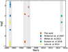 |
Fig. 8. Ionisation parameters of the warm absorbers identified in Mrk 766 over the years. The results from this work are shown in red. The higher ionised absorber found in this work seems agree with other WAs found in the literature, while our less ionised WA does not correlate with others that were found previously. |
5.1.4. Warm absorber distance estimation
The location of WAs in AGN is unconstrained in general. However, based on various assumptions regarding the morphology and other aspects of these X-ray absorbers, it is possible to place constraints on the lower and upper limit of the locations of individual WAs the system (Blustin et al. 2005).
The first assumption that is required is that the depth of the X-ray absorber, Δr, should not exceed the distance at which the absorber lies from the source (Reynolds & Fabian 1995). In this way, taking the hydrogen column density to be NH = nΔrf, where n represents the column density of the gas, and f the filling factor, we followed the method outlined in Blustin et al. (2005) and used the parameters of our best-fit model alongside the ionising luminosity obtained from the EPIC-pn and OM data (log Lion = 44.20) to obtain the upper limits for the distances at which the WAs may be found.
Therefore, the upper limit for the WA lying at log ξ = 2.15 ± 0.05 was found to be at a distance from the ionising source of r ≤ 395 pc, while the WA at a log ξ = −0.58 ± 0.11 obtained a looser constraint with an upper limit of r ≤ 2 × 10⁶ pc. This latter constraint would place this WA outside the host galaxy boundaries. However, this outflow might be a Galaxy-scale outflow, which is seen as a warm absorber in the X-ray band, such as those in 1H 0419-577 (Di Gesu et al. 2017).
To be able to calculate the lower limit of the absorber positions, we must assume that the outflowing velocity is higher than or equal to the escape velocity. For both of the WAs, we adopted the upper limits on vout (Table 3). Adopting a black hole mass of 1.26 × 10⁶ M⊙ (Giacchè et al. 2014), we obtained r ≥ 0.90 pc and r ≥ 1.08 pc for the log ξ = −0.58 ± 0.11 and log ξ = 2.15 ± 0.05 absorbers, respectively.
5.2. Emission lines
It is not possible to distinguish on a statistical basis whether the emitting gas is part of the absorbing gas or if it is a separate, unabsorbed component. However, comparing the values of the individual PION parameters with those of the WAs, it became apparent that the log ξ of the emission plasma was not consistent within more than 3σ with the ionisation parameter of WA1 and WA2. This in itself indicated that this emission might not be linked to the WAs, making Case 1 less likely (see Sect. 4.2). Moreover, we do not expect the emission lines to display a significant outflow velocity for either scenario. We found this component to have a log ξ = 1.56 ± 0.05 and NH = (9.00 ± 0.61)×1022 cm−2, as well as an outflowing velocity consistent with zero, and an aperture angle Ω/4π = (3.84 ± 1.31)×10−3, which is consistent with the idea that the detected emission was produced in a narrow cone within the NLR. Using PION allowed us to detect emission from H and He-like transitions of N, O, C, and Ne as well as the RRCs of O VII, and O VIII. The detection of these narrow RRCs implies that the gas that creates this emission must be photoionised. Accordingly, an association of the emitting gas with the absorbing CIA is unlikely because RRCs tend to be broad features for hot collisionally ionised plasmas, but are narrow features for cooler photoionised plasmas (Liedahl & Paerels 1996; Liedahl 1999). Moreover, an independent fit of the narrow RRC features (RRC model in SPEX) indicates that they originated at a low temperature (6.0 ± 0.2 eV). This temperature is associated with a photoionised gas, which is consistent with the PION modelling. Additionally, this would disfavour an association with the CIA component because in that case, we would have expected broadened RRC features.
The tight degeneracy between the distance from the ionising source and the gas density implies that when we assume that this gas is located in the NLR (100 pc), then, given its ionisation parameter, the density must be low (1 × 103 cm−3) in order to have such a high ionising parameter. The emitting gas might also be far from our line of sight, but closer to the black hole than the WA. Fig. 9 shows this scenario and illustrates all physical absorbing and emitting components that make up the model.
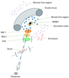 |
Fig. 9. Depiction of the emission for Case 2, where the emission is not linked to the WAs and is created away from our line of sight. Therefore, it is not absorbed by the components of the source and host galaxy. The CIA is placed within brackets to show that this position is only a placeholder because based on our analysis, we were unable to constrain its position with respect to the rest of the system. The key parts of the AGN are clearly labelled, while the different absorbing components are given different colours and patterns to differentiate them. |
6. Conclusions
We analysed the high-energy resolution X-ray spectrum of the narrow-line Seyfert 1 galaxy Mrk 766 using four observations taken with XMM-Newton in 2005 to investigate the properties of the complex ionised absorber / emitter along the line of sight as well as the absorption by dust intrinsic to the source. The conclusions based on our findings are listed below.
-
Two distinct phases of WAs are present in Mrk 766, with log ξ = 2.15 ± 0.05 and log ξ = −0.58 ± 0.11. They have moderate outflowing velocities with vout = 60 ± 40 and vout ≤ 110 km s−1, and they both partially cover the source with CV = 0.85 ± 0.09 and CV ≤ 1, indicating potential stratification in their structure.
-
We found evidence for a collisionally ionised absorber in Mrk 766 with T = 50.7 ± 3.2 eV and NH = (8.17 ± 0.31)×1021 cm−2. We found its velocity to be vout = 250 ± 70 km s−1. This might be created by a shocked interface between a WA and the host galaxy, or by ionised gas that was shocked against the ISM.
-
A dust component is present in Mrk 766. This dust might not be associated with the host galaxy, but rather with more nuclear regions of the system.
-
We found emission in the spectrum of Mrk 766 that is likely created by a photoionised gas with log ξ = 1.56 ± 0.05 in the NLR.
Acknowledgments
We thank the anonymous referee for their thorough reading and for their very useful comments and suggestions that have improved the clarity of the paper.
References
- Akaike, H. 1974, IEEE Trans. Automat. Control, 19, 716 [Google Scholar]
- Behar, E., Rasmussen, A. P., Blustin, A. J., et al. 2003, ApJ, 598, 232 [Google Scholar]
- Bianchi, S., Guainazzi, M., & Chiaberge, M. 2006, A&A, 448, 499 [NASA ADS] [CrossRef] [EDP Sciences] [Google Scholar]
- Blustin, A. J., Branduardi-Raymont, G., Behar, E., et al. 2002, A&A, 392, 453 [NASA ADS] [CrossRef] [EDP Sciences] [Google Scholar]
- Blustin, A. J., Page, M. J., Fuerst, S. V., Branduardi-Raymont, G., & Ashton, C. E. 2005, A&A, 431, 111 [CrossRef] [EDP Sciences] [Google Scholar]
- Bohlin, R. C., Savage, B. D., & Drake, J. F. 1978, ApJ, 224, 132 [Google Scholar]
- Branduardi-Raymont, G., Sako, M., Kahn, S. M., et al. 2001, A&A, 365, L140 [NASA ADS] [CrossRef] [EDP Sciences] [Google Scholar]
- Buisson, D. J. K., Parker, M. L., Kara, E., et al. 2018, MNRAS, 480, 3689 [NASA ADS] [CrossRef] [Google Scholar]
- Burnham, K. P., & Anderson, D. R. 2002, Model Selection and Multimodel Inference: A Practical Information-theoretic Approach, 2nd edn. (Springer) [Google Scholar]
- Cardelli, J. A., Clayton, G. C., & Mathis, J. S. 1989, ApJ, 345, 245 [Google Scholar]
- Cash, W. 1979, ApJ, 228, 939 [Google Scholar]
- Costantini, E. 2010, Space Sci. Rev., 157, 265 [NASA ADS] [CrossRef] [Google Scholar]
- Costantini, E., & Corrales, L. 2022, in Interstellar Absorption and Dust Scattering, eds. C. Bambi, & A. Santangelo (Singapore: Springer Nature), 1 [Google Scholar]
- Costantini, E., Gallo, L. C., Brandt, W. N., Fabian, A. C., & Boller, T. 2007, MNRAS, 378, 873 [NASA ADS] [CrossRef] [Google Scholar]
- Crenshaw, D. M., & Kraemer, S. B. 2012, ApJ, 753, 75 [NASA ADS] [CrossRef] [Google Scholar]
- den Herder, J. W., Brinkman, A. C., Kahn, S. M., et al. 2001, A&A, 365, L7 [NASA ADS] [CrossRef] [EDP Sciences] [Google Scholar]
- Di Gesu, L., Costantini, E., Piconcelli, E., et al. 2017, A&A, 608, A115 [NASA ADS] [CrossRef] [EDP Sciences] [Google Scholar]
- Done, C., Davis, S. W., Jin, C., Blaes, O., & Ward, M. 2012, MNRAS, 420, 1848 [Google Scholar]
- Ebrero, J., Costantini, E., Kaastra, J. S., et al. 2010, A&A, 520, A36 [NASA ADS] [CrossRef] [EDP Sciences] [Google Scholar]
- Fabian, A. 2012, ARA&A, 50, 455 [CrossRef] [Google Scholar]
- Falco, E. E., Kurtz, M. J., Geller, M. J., et al. 1999, PASP, 111, 438 [Google Scholar]
- George, I. M., Turner, T. J., Netzer, H., et al. 1998, ApJS, 114, 73 [NASA ADS] [CrossRef] [Google Scholar]
- Giacchè, S., Gilli, R., & Titarchuk, L. 2014, A&A, 562, A44 [NASA ADS] [CrossRef] [EDP Sciences] [Google Scholar]
- Gonzalez Delgado, R. M., & Perez, E. 1996, MNRAS, 278, 737 [NASA ADS] [CrossRef] [Google Scholar]
- Gordon, K. D., Clayton, G. C., Misselt, K. A., Landolt, A. U., & Wolff, M. J. 2003, ApJ, 594, 279 [NASA ADS] [CrossRef] [Google Scholar]
- Grasha, K., Chen, Q. H., Battisti, A. J., et al. 2022, ApJ, 929, 118 [NASA ADS] [CrossRef] [Google Scholar]
- Guainazzi, M., & Bianchi, S. 2007, MNRAS, 374, 1290 [Google Scholar]
- Heckman, T. M., & Best, P. N. 2014, ARA&A, 52, 589 [Google Scholar]
- Hopkins, P. F., Strauss, M. A., Hall, P. B., et al. 2004, AJ, 128, 1112 [Google Scholar]
- Hopkins, P. F., Hernquist, L., Cox, T. J., et al. 2005, ApJ, 630, 705 [NASA ADS] [CrossRef] [Google Scholar]
- Jansen, F., Lumb, D., Altieri, B., et al. 2001, A&A, 365, L1 [NASA ADS] [CrossRef] [EDP Sciences] [Google Scholar]
- Kaastra, J. S. 2017, A&A, 605, A51 [NASA ADS] [CrossRef] [EDP Sciences] [Google Scholar]
- Kaastra, J. S., Mewe, R., & Nieuwenhuijzen, H. 1996, in UV and X-ray Spectroscopy of Astrophysical and Laboratory Plasmas, eds. K. Yamashita, & T. Watanabe, 411 [Google Scholar]
- Kaastra, J. S., Mewe, R., Liedahl, D. A., Komossa, S., & Brinkman, A. C. 2000, A&A, 354, L83 [NASA ADS] [Google Scholar]
- Kaspi, S., Netzer, H., Chelouche, D., et al. 2004, ApJ, 611, 68 [NASA ADS] [CrossRef] [Google Scholar]
- King, A., & Pounds, K. 2015, ARA&A, 53, 115 [NASA ADS] [CrossRef] [Google Scholar]
- Kinkhabwala, A., Sako, M., Behar, E., et al. 2002, ApJ, 575, 732 [Google Scholar]
- Kubota, A., & Done, C. 2018, MNRAS, 480, 1247 [Google Scholar]
- Laha, S., Guainazzi, M., Dewangan, G. C., Chakravorty, S., & Kembhavi, A. K. 2014, MNRAS, 441, 2613 [NASA ADS] [CrossRef] [Google Scholar]
- Laha, S., Reynolds, C. S., Reeves, J., et al. 2020, Nat. Astron., 5, 13 [Google Scholar]
- Lee, J. C., Ogle, P. M., Canizares, C. R., et al. 2001, ApJ, 554, L13 [NASA ADS] [CrossRef] [Google Scholar]
- Lee, J. C., Kriss, G. A., Chakravorty, S., et al. 2013, MNRAS, 430, 2650 [NASA ADS] [CrossRef] [Google Scholar]
- Leighly, K. M., Mushotzky, R. F., Yaqoob, T., Kunieda, H., & Edelson, R. 1996, ApJ, 469, 147 [Google Scholar]
- Liedahl, D. A. 1999, in X-Ray Spectroscopy in Astrophysics, eds. J. van Paradijs, & J. A. M. Bleeker (Berlin, Heidelberg: Springer), 189 [Google Scholar]
- Liedahl, D. A., & Paerels, F. 1996, ApJ, 468, L33 [Google Scholar]
- Longinotti, A. L., Krongold, Y., Kriss, G. A., et al. 2013, ApJ, 766, 104 [NASA ADS] [CrossRef] [Google Scholar]
- Maksym, W. P., Fabbiano, G., Elvis, M., et al. 2019, ApJ, 872, 94 [NASA ADS] [CrossRef] [Google Scholar]
- Malkan, M. A., Gorjian, V., & Tam, R. 1998, ApJS, 117, 25 [Google Scholar]
- Mason, K. O., Breeveld, A., Much, R., et al. 2001, A&A, 365, L36 [NASA ADS] [CrossRef] [EDP Sciences] [Google Scholar]
- Mason, K. O., Branduardi-Raymont, G., Ogle, P. M., et al. 2003, ApJ, 582, 95 [Google Scholar]
- McKernan, B., Yaqoob, T., & Reynolds, C. S. 2007, MNRAS, 379, 1359 [NASA ADS] [CrossRef] [Google Scholar]
- Mehdipour, M., & Costantini, E. 2018, A&A, 619, A20 [NASA ADS] [CrossRef] [EDP Sciences] [Google Scholar]
- Mehdipour, M., Branduardi-Raymont, G., & Page, M. J. 2010, A&A, 514, A100 [NASA ADS] [CrossRef] [EDP Sciences] [Google Scholar]
- Mehdipour, M., Branduardi-Raymont, G., Kaastra, J. S., et al. 2011, A&A, 534, A39 [NASA ADS] [CrossRef] [EDP Sciences] [Google Scholar]
- Mehdipour, M., Kaastra, J. S., & Kallman, T. 2016, A&A, 596, A65 [NASA ADS] [CrossRef] [EDP Sciences] [Google Scholar]
- Miller, J. M., Kaastra, J. S., Miller, M. C., et al. 2015, Nat, 526, 542 [Google Scholar]
- Nagar, N. M., Wilson, A. S., Mulchaey, J. S., & Gallimore, J. F. 1999, ApJS, 120, 209 [Google Scholar]
- Ogorzalek, A., King, A. L., Allen, S. W., Raymond, J. C., & Wilkins, D. R. 2022, MNRAS, 516, 5027 [Google Scholar]
- Paggi, A., Wang, J., Fabbiano, G., Elvis, M., & Karovska, M. 2012, ApJ, 756, 39 [NASA ADS] [CrossRef] [Google Scholar]
- Pounds, K. A., & King, A. R. 2013, MNRAS, 433, 1369 [NASA ADS] [CrossRef] [Google Scholar]
- Pounds, K. A., & Vaughan, S. 2011, MNRAS, 413, 1251 [Google Scholar]
- Psaradaki, I., Mehdipour, M., Rogantini, D., et al. 2024, ApJ, accepted [arXiv:2411.02270] [Google Scholar]
- Reynolds, C. S., & Fabian, A. C. 1995, MNRAS, 273, 1167 [NASA ADS] [CrossRef] [Google Scholar]
- Riffel, R., Rodríguez-Ardila, A., & Pastoriza, M. G. 2006, A&A, 457, 61 [NASA ADS] [CrossRef] [EDP Sciences] [Google Scholar]
- Risaliti, G., Nardini, E., Salvati, M., et al. 2010, MNRAS, 410, 1027 [Google Scholar]
- Rodríguez-Ardila, A., Contini, M., & Viegas, S. M. 2005, MNRAS, 357, 220 [CrossRef] [Google Scholar]
- Sako, M., Kahn, S. M., Branduardi-Raymont, G., et al. 2003, ApJ, 596, 114 [NASA ADS] [CrossRef] [Google Scholar]
- Schlafly, E. F., & Finkbeiner, D. P. 2011, ApJ, 737, 103 [Google Scholar]
- Shakura, N. I., & Sunyaev, R. A. 1973, A&A, 24, 337 [NASA ADS] [Google Scholar]
- Silk, J., & Rees, M. J. 1998, A&A, 331, L1 [NASA ADS] [Google Scholar]
- Silva, C. V., Costantini, E., Giustini, M., et al. 2018, MNRAS, 480, 2334 [NASA ADS] [CrossRef] [Google Scholar]
- Steenbrugge, K. C., Kaastra, J. S., Crenshaw, D. M., et al. 2005, A&A, 434, 569 [NASA ADS] [CrossRef] [EDP Sciences] [Google Scholar]
- Turner, M. J. L., Abbey, A., Arnaud, M., et al. 2001, A&A, 365, L27 [CrossRef] [EDP Sciences] [Google Scholar]
- Turner, T. J., Miller, L., Reeves, J. N., & Kraemer, S. B. 2007, A&A, 475, 121 [NASA ADS] [CrossRef] [EDP Sciences] [Google Scholar]
- Ulvestad, J. S., Antonucci, R. R. J., & Goodrich, R. W. 1995, AJ, 109, 81 [NASA ADS] [CrossRef] [Google Scholar]
- van Peet, J. C. A., Costantini, E., Méndez, M., Paerels, F. B. S., & Cottam, J. 2009, A&A, 497, 805 [NASA ADS] [CrossRef] [EDP Sciences] [Google Scholar]
- Vasudevan, R. V., Mushotzky, R. F., Winter, L. M., & Fabian, A. C. 2009, MNRAS, 399, 1553 [NASA ADS] [CrossRef] [Google Scholar]
- Wang, J., Fabbiano, G., Elvis, M., et al. 2011, ApJ, 736, 62 [NASA ADS] [CrossRef] [Google Scholar]
- Winter, L. M., Veilleux, S., McKernan, B., & Kallman, T. R. 2012, ApJ, 745, 107 [NASA ADS] [CrossRef] [Google Scholar]
- Yao, Y., & Wang, Q. D. 2006, ApJ, 641, 930 [CrossRef] [Google Scholar]
- Zycki, P. T., Done, C., & Smith, D. A. 1999, MNRAS, 305, 231 [Google Scholar]
All Tables
All Figures
|
Fig. 1. Spectra of Mrk 766 taken with the XMM-Newton EPIC-pn instrument. The different observations taken during the 2005 campaign are shown in various colours. We show observations that were not included in the study in grey. We plot the merged spectrum of observations 301, 401, 501, and 601 in red. We refer to the observations by the last three digits of their observation IDs. |
| In the text | |
|
Fig. 2. Spectra of Mrk 766 taken with the XMM-Newton OM instrument. The different observations used for this study are shown in various colours. The OM filters from left to right are B, U, UVW1, UVM2, and UVW2. We refer to the observations by the last three digits of their observation IDs. |
| In the text | |
|
Fig. 3. Model obtained from the SED fitting of the XMM-Newton EPIC-pn and OM merged observations. We show the best-fit model to the data in black. The curves in grey show the emission components that make up the model, which are from left to right DBB, COMT, POW, REFL, and GAUSS. The model of the absorbed spectrum is plotted in blue. |
| In the text | |
|
Fig. 4. Merged RGS data in black. We indicate the regions in which we expect ions of a certain element in the spectrum with horizontal lines. Features marked in yellow correspond to Galactic features, and blue indicates regions in which absorption / emission features by certain elements is expected. |
| In the text | |
|
Fig. 5. Comparison between a model using a combination of three WAs and dust as opposed to WAs alone. Upper panel: Model implementing three WAs and dust (red) vs. WAs alone (blue). The latter case does not take into account the additional absorption in the 15 − 18 Å region, while the WAs and dust model does. The RGS data are shown in black. Middle panel: Residuals of the WA and dust model. Lower panel: Residuals of the WA model. |
| In the text | |
|
Fig. 6. Comparison between a model using a combination of WAs and CIA as opposed to WAs alone. Upper panel: Transmission plot. Transmission is defined as the observed spectrum divided by the continuum. This plot compares the behaviour of the CIA (red) around the 13 − 20 Å region in comparison to a WA with log ξ ∼ 0.96 (blue). The transmissions obtained by the other WAs used in both models are shown in fainter red and blue. Upper middle panel: Difference between a model implementing WAs and CIA (red) as opposed to WAs alone (blue). “WAs and CIA” is used to indicate our best-fit model. “WAs” is meant to represent the model with three WAs and no CIA. It is apparent that the latter case creates additional absorption in the 17 − 18 Å region. The most prominent absorption features identified by our models are marked and labelled. Lower middle panel: Residuals of the CIA and WA model. Lower panel: Residuals of the WAs model. |
| In the text | |
|
Fig. 7. Best fit model for the RGS data. Upper panel: Transmission plot. Transmission is defined as the observed spectrum divided by the continuum. The different absorbing components are explained in the legend. Middle upper panel: RGS data (black) with the best-fit model (red). Middle lower panel: Residuals from our best-fit model. Lower panel: Emission features predicted by PION in emission. The most prominent features are labelled. |
| In the text | |
|
Fig. 8. Ionisation parameters of the warm absorbers identified in Mrk 766 over the years. The results from this work are shown in red. The higher ionised absorber found in this work seems agree with other WAs found in the literature, while our less ionised WA does not correlate with others that were found previously. |
| In the text | |
|
Fig. 9. Depiction of the emission for Case 2, where the emission is not linked to the WAs and is created away from our line of sight. Therefore, it is not absorbed by the components of the source and host galaxy. The CIA is placed within brackets to show that this position is only a placeholder because based on our analysis, we were unable to constrain its position with respect to the rest of the system. The key parts of the AGN are clearly labelled, while the different absorbing components are given different colours and patterns to differentiate them. |
| In the text | |
Current usage metrics show cumulative count of Article Views (full-text article views including HTML views, PDF and ePub downloads, according to the available data) and Abstracts Views on Vision4Press platform.
Data correspond to usage on the plateform after 2015. The current usage metrics is available 48-96 hours after online publication and is updated daily on week days.
Initial download of the metrics may take a while.