| Issue |
A&A
Volume 538, February 2012
|
|
|---|---|---|
| Article Number | A124 | |
| Number of page(s) | 17 | |
| Section | Astrophysical processes | |
| DOI | https://doi.org/10.1051/0004-6361/201118182 | |
| Published online | 14 February 2012 | |
Grain charging in protoplanetary discs
Max-Planck-Institut für Astronomie, Königstuhl 17, 69117 Heidelberg, Germany
e-mail: ilgner@mpia-hd.mpg.de
Received: 29 September 2011
Accepted: 26 November 2011
Context. Recent work identified a growth barrier for dust coagulation that originates in the electric repulsion between colliding particles. Depending on its charge state, dust material may have the potential to control key processes towards planet formation such as magnetohydrodynamic (MHD) turbulence and grain growth, which are coupled in a two-way process.
Aims. We quantify the grain charging at different stages of disc evolution and differentiate between two very extreme cases: compact spherical grains and aggregates with fractal dimension Df = 2.
Methods. Applying a simple chemical network that accounts for collisional charging of grains, we provide a semi-analytical solution. This allowed us to calculate the equilibrium population of grain charges and the ionisation fraction efficiently. The grain charging was evaluated for different dynamical environments ranging from static to non-stationary disc configurations.
Results. The results show that the adsorption/desorption of neutral gas-phase heavy metals, such as magnesium, effects the charging state of grains. The greater the difference between the thermal velocities of the metal and the dominant molecular ion, the greater the change in the mean grain charge. Agglomerates have more negative excess charge on average than compact spherical particles of the same mass. The rise in the mean grain charge is proportional to N1/6 in the ion-dust limit. We find that grain charging in a non-stationary disc environment is expected to lead to similar results.
Conclusions. The results indicate that the dust growth and settling in regions where the dust growth is limited by the so-called “electro-static barrier” do not prevent the dust material from remaining the dominant charge carrier.
Key words: accretion, accretion disks / circumstellar matter / protoplanetary disks / stars: pre-main sequence
© ESO, 2012
1. Introduction
Small dust particles are regarded as the key ingredient to control the planet formation process in protoplanetary discs. At early stages of planet formation, submicron-sized compact particles are thought to grow towards larger but fluffy agglomerates. At mm to cm sizes these agglomerates are supposed to be compacted, whereby they loose their fractal structure. Because of the rise in the mass-to-surface ratio associated with the compaction, agglomerates tend to be more concentrated locally. However, there are a number of potential processes that may control grain growth, one of which is disc turbulence. The magnetorotational instability – MRI – (Balbus & Hawley 1991; Hawley & Balbus 1991) has been shown to be robust in generating turbulence in Keplerian discs. MHD turbulence provides the internal stress required for mass accretion, the rate of which is constrained by observations. Observations of young stars indicate that discs usually show signatures of active gas accretion onto the central star with mass flow rates of about 10−8 ± 1 M⊙ yr-1 (e.g., Sicilia-Aguilar et al. 2004). Recent observations from discs around young stars also set constraints on the turbulent linewidth and provide support for subsonic turbulence in discs (Hughes et al. 2011). However, numerical studies (e.g. Fleming & Stone 2003) on MRI-driven MHD turbulence have identified locations within the planet forming regions, the so-called “dead zones”, where the coupling between the gas and the magnetic field is not sufficient to maintain MHD turbulence. Fleming & Stone also showed that a low Reynolds stress can be maintained in the dead zone, such that low levels of accretion are sustained there. That is why dead zones have been considered to advance the planet formation process. Dead zones provide a safe environment for grain growth and for planetesimals (Gressel et al. 2011). However, the presence of small grains in the weakly ionized dead zones leads to significant changes in the abundances of the charge carriers in the gas phase and therefore affects the MRI. In other words, MHD turbulence and grain growth are coupled in a two-way process.
Grain charging may also effect the dust growth: Okuzumi (2009) pointed out that the so-called “electro-static barrier” may inhibit dust coagulation in planet forming regions. In a subsequent study, Okuzumi et al. (2011a) extended the analysis including the dust size distribution. They found that under certain conditions the dust undergoes bimodal growth. While the small aggregates sweep up free electrons, the large aggregates continue to grow. However, the growing stalls if the electrostatic repulsion becomes strong and the collisions are driven by Brownian motion. The results of Okuzumi et al. (2011b) indicate that under minimum mass solar nebula conditions the dust growth halts at aggregate sizes beyond [4 × 10-5,3 × 10-2] cm depending on the radial position. Conventional chemical models studying the dust-grain chemistry in protoplanetary discs account for up to |Z| = 3 grain charges (e.g. Sano et al. 2000). More recently, the range of grain charges was extended considerably for various purposes. Focusing on surface layers of T-Tauri and transitional discs, Perez-Becker & Chiang (2011) examined the charge distribution on grains covering grain charges [Zmin,Zmax] = [−200,200] . Okuzumi (2009) calculated the charge distribution on dust aggregates. He demonstrated that aggregates made of N = 1010 monomers can carry excess charges of about Zmin ~ − 105. To account for higher grain charges we therefore improved our simple chemical network introduced in Ilgner & Nelson (2006a) allowing [Zmin,Zmax] to become free of choice and appropriate to the conditions applied.
In this paper we examine the grain charging for various stages of disc evolution ranging from static to non-stationary disc environment. Linking the grain charging with the gas-dust dynamics provides a natural environment to mimic the variation of the dust-to-gas ratio Σd/Σg. The grain charging is assumed to originate in collisional charging processes between grains, electrons, and gas-phase ions. We include X-ray ionisation from the central star as the primary source for ionisation and consider, to some extent, the contributions from cosmic ray particles. We furthermore assume an equilibrium distribution of dust material in vertical direction balancing turbulent stirring and sedimentation. In particular, we apply the model of Takeuchi & Lin (2005) to simulate the dynamics of the gas-dust disc. One of our primary goals is to compare the grain charging obtained for compact spheres and dust agglomerates and the mean grain charge in particular.
We have investigated the effect that thermal adsorption/desorption of metals has on grain charging using two different chemical networks. In comparison with the values obtained by switching off the thermal adsorption of metals, the modified Oppenheimer-Dalgarno model produces lower, the Umebayashi-Nakano model higher values for the mean grain charge. This originates in differences in the thermal velocities of the dominant gas-phase ion:  . In line with expectations, we find that dust agglomerates have a higher charge-to-mass ratio carrying more charges than the corresponding compact spherical particles. Considering stationary disc configurations, we observe that grain charging on dust agglomerates is always associated with the so-called “ion-dust regime”, where the charge balance is mainly maintained by negatively charged grains and positively charged gas-phase ions. (The ion-electron regime is characterised by the balance between gas-phase ions and electrons.) In particular, we show that the fractional abundances of the charge carriers are independent of the number N of constituent monomers. Concerning compact spherical dust particles, we identified regions z/hg > 0 associated with the ion-electron regime. Another conclusion of our work is that – for the parameter range considered (i.e., compact radii a∗ ≤ 10-3 cm and agglomerates with characteristic radii ac ≤ 10-2 cm with N ≤ 106, respectively1) – grain charging in a non-stationary disc environment is expected to lead to similar results. We also present semi-analytical solutions for both agglomerates and compact spheres that allow us to determine the equilibrium distribution of ⟨ Z ⟩ ,
  , and the fractional abundances of the charge carriers a priori.
The paper is organised as follows. In Sect. 2 we discuss the disc model we apply. In Sect. 3 we introduce the chemical network that we used to compare our results with the reaction network Okuzumi (2009) applied. Key problems concerning the ionisation rates are discussed in Sect. 4 while the numerical methods applied are described in Sect. 5. In Sect. 6 we present the results of our model, and finally in Sect. 7 we summarise the key findings of our study.
2. Disc model
The geometry of the disc model is described in cylindrical coordinates (R,ϕ,z), where R,ϕ, and z denote the radial distance to the point of interest, the azimuthal angle, and the height. Here, we simply considered a two-dimensional (2D) geometry by assuming axial symmetry, i.e., ∂/∂ϕ = 0.
Treating the disc as a two-component fluid of dust particles and gas, we assumed that the circumstellar gas disc is turbulent and accreting onto the central star. We also assumed that the gas is primarily heated by stellar radiation rather than viscous dissipation. We supposed that the mean gas motion is characterised by a subsonic flow in R, supersonic flow in ϕ, while the gas density is characterised by hydrostatic equilibrium in z-direction.
The underlying disc model we applied is based on the assumption of a two-component fluid that allows the dust particles and the gas to follow different velocity fields vd and vg, respectively. In particular, we considered dust particles for which the two-component fluid is best described in the so-called “free molecular approximation”, e.g.,  cm under minimum mass solar nebula condition. (a0 denotes the dust radius while Rau is the orbital radius in units of AU.) Since the mean free path of the gas molecules exceeds the dust particle sizes, the collisions between the gas and the dust particles are much more frequent than the collisions between gas particles. We moreover considered disc stages for which the gas density ϱg dominates over the density ϱd of the dust. The gas is therefore assumed to be decoupled from the dust disc. However, the gas drag may alter the velocity vd of the dust particles. Assuming vd ≪ cs, the drag coefficient β is characterised by (Epstein 1924)
  (1)where vth denotes the thermal velocity. We can additionally specify the friction or stopping time tS = m/β, which will turn out to be an important diagnostic quantity. m and σ refer to the mass of the dust particle and its projected surface area, respectively. The friction time basically characterises the time scale needed to couple the dust dynamics with the gas, which is why tS is also called stopping time. Instead of tS, we used the dimensionless stopping time TS defined as the ratio between tS and the dynamical time scale tϕ.
We studied the grain charging for various stages of disc evolution ranging from static to non-stationary disc environment. A description of the gas-dust dynamics applied is given in Sect. 2.1 while Sect. 2.2 summarises the local disc structure.
2.1. Dynamics of the gas-dust disc
The extreme case of disc dynamics is associated with the so-called “minimum mass solar nebula” (MMSN) model, which was proposed by Hayashi (1981). He adopted the following radial profiles of the dust and gas surface densities Σd and Σg for R < 36 AU 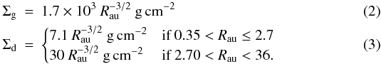 We recall that Hayashi derived the power law above assuming no substantial transport of dust material. Although recent simulations of the radial migration of planets indicate that the radial profile of Σg (as well as the gas temperature profile) differs significantly from the MMSN model (cf. Desch 2007), we opted for Hayashi’s MMSN model. That is because the assumed power index for the MMSN model nicely corresponds to a static solution of the disc model of Takeuchi & Lin (2002), see below for more information. The grain charging obtained for that particular environment is discussed in Sect. 3.
Takeuchi & Lin (2005) extended their disc model to study the dynamical evolution of the gas-dust disc. The corresponding set of continuity equations is 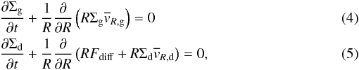 where
where  and
and  are the vertically integrated velocities of the gas and the dust particles. The (ordinary) diffusion is described by the phenomenological equation, which is well-known as Fick’s first law for a binary system. The corresponding mass flow is approximated by
 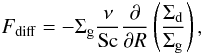 (6)with the Schmidt number
  specifying the ratio of the rate of angular momentum transport to the rate of turbulent transport of grain particles. We used the α prescription for the viscous stress, such that the kinematic viscosity is ν = αcshg.
The interpretation of the integrated velocities and is crucial for our understanding of the species’ transport in our particular model. and refer rather to the velocities associated with the transport of the surface densities Σg and Σd than to the velocities the individual species are transported with. For the gas disc, the velocity can be obtained by combining the equation of angular momentum and the continuity equation 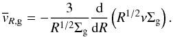 (7)Inserting Eq. (7) into the continuity equation for the gas surface density, we obtain the well-known diffusion equation reviewed, e.g., in Pringle (1981).
Assuming power laws for the pressure scale height hg, the sound speed cs, and the local gas density ϱg (see Sect. 2.2 below), Takeuchi & Lin (2002) have presented steady-state solutions of Eqs. (4), (5). Evaluating the mass fluxes  and
and  , they obtained Σg ∝ R − 3/2 for vR,g/cs = 0 and
 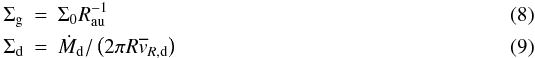 for vR,g/cs ≠ 0 where the mass flux Ṁd of dust material enters as a free parameter.
 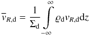 (10)can an be calculated semi-analytically (see Takeuchi & Lin 2002) assuming
 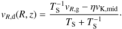 (11)Here, η and vK,mid refer to the ratio of the pressure gradient to the gravity and Keplerian velocity at disc midplane, respectively.
However, apart from steady-state conditions it is difficult to find a reliable approximation for . We followed the instruction of Takeuchi & Lin (2005) to calculate but we are aware of the caveats inherent in their approach. This problem arises because a general analytical expression for the corresponding radial component vR,g of the gas velocity field does not exist. In order to tackle this problem we simply approximate by 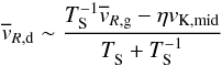 (12)evaluating TS and η at disc midplane:
 ![\begin{eqnarray} \eta & = & - \left( \frac{h_{\rm g}}{R} \right)^2 \left( \frac{\partial \ln \Sigma_{\rm g}}{\partial \ln R} + \frac{q - 3}{2} \right) \label{eq13:sec2} \\[.3em] T_{\rm S} & = & \frac{3}{8} \frac{\pi}{\Sigma_{\rm g}} \frac{m}{\sigma} , \label{eq14:sec2} \end{eqnarray}](/articles/aa/full_html/2012/02/aa18182-11/aa18182-11-eq70.png) where q denotes the power index associated with the gas pressure scale height hg (see next subsection).
where q denotes the power index associated with the gas pressure scale height hg (see next subsection).
As we will demonstrate below, the dynamics of the gas-dust disc is controlled by the stopping time TS. Because of TS ∝ m/σ the stopping time relies on the particular topology of the dust particles considered. We studied two extreme cases of grain topology: compact spherical grains and irregular, very porous dust agglomerates. We begin addressing that particular question for compact spherical grains before discussing the dust agglomerates and its effect on the gas-dust dynamics.
Case A: Compact spherical dust grains Considering compact spherical grain particles of material bulk density ϱp and a radius a0, the stopping time at disc midplane z/hg = 0 is given by
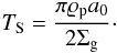 Takeuchi & Lin (2005) studied in detail the effect of compact spherical grains on the dynamics of the gas-dust disc. We took their fiducial model, which nicely demonstrates the inward migration of larger (spherical) dust particles to test our implementation of the numerical schemes applied. We also adopted boundary and initial conditions suitable for our particular model2. To summarise, we set the inner boundary at Rinner = 0.1 AU and replaced the zero torque boundary conditions with predefined analytical values for Σg(t). In particular, we applied the self-similarity solution
 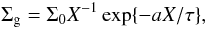 (15)Lynden-Bell & Pringle (1974) obtained under the assumption νt ∝ R with dimensionless variables X = R/R0 and τ = t/t0 + 1. In the limit of X ≪ 1 the expression reduces to Σg ∝ X-1, which represents the steady-state solution Σg ∝ R-1 discussed above. The most appropriate value for the constant a was applied to approximate Σg(t) in the outer disc regions. We replaced the initial assumption Σd/Σg = const. by |Ṁd| = const. For the sake of convenience we applied the value of Takeuchi & Lin (2002) Ṁd = 10-10 M⊙ yr-1, which is one order of magnitude smaller than the corresponding mass flux of the gas Ṁg = 3πνΣg ~ 2.6 × 10⁻⁹ M⊙ yr-1.
Because of TS ∝ a0, the dynamics of the dust disc depends on the size of the spherical grain particle considered. This may also have important consequences for the dust growth. The simplest approach to mimic the dust growth is to assume that the entire available dust mass is represented by monodisperse compact spherical particles of a given size a∗. By changing a∗ one may trace different stages of dust growth. However, dust growth is supposed to be processed by coagulation leading to irregular dust agglomerates. The effect of dust agglomerates on the dust dynamics is discussed below.
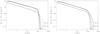 |
Fig. 1 Radial profile of the surface densities of the gas and the dust at different time snaps t = 105,3 × 10⁵ and 106 yr. The solid lines correspond to the dust surface density while the gas surface density is shown using the dashed lines. The (red-coloured) dotted line refers to Σg ~ R-1 and Σd = Ṁd/(2πR < vR,d > ) at t/tK = 0. |Ṁd| = 10-10 M⊙/yr, α = 10-3, and ϱp = 1.0 g cm-3. The profiles shown in the left panel are obtained under the assumption of spherical grains with a0 = 10-3 cm. The corresponding profiles obtained for agglomerates with DBCCA = 2 and N = 106 monomers of a0 = 10-5 cm are shown in the right panel. |
Case B: Irregular porous dust agglomerates The grain particles are now regarded as dust agglomerates. In particular, we considered agglomerates associated with the so-called “ballistic cluster-cluster aggregation” (BCCA) model. The BCCA model describes the growth of aggregates3 through collisions of equal-sized aggregates as cartooned in Fig. 2. We are aware of constraints associated with the BCCA growth process (see discussion in Okuzumi 2009). However, for the purpose of our paper we simply assumed that BCCA agglomerates are formed independently of the disc environment applied. That is because the BCCA agglomerates are used as test particles to trace the grain charging for different disc environments.
Simulations of dust growth have shown that for the BCCA model the characteristic radius4ac obeys a power law (e.g., Okuzumi et al. 2009) while the mean value for the projected surface area is well approximated by a linear function of N (cf. Minato et al. 2006):  N denotes the number of the constituent monomers forming the agglomerate (a0 is the radius of each monomer). DBCCA is the fractal dimension of BCCA associated with ac and DBCCA ≈ 1.9 (Meakin 1991). We considered DBCCA = 2. The projected surface area is
  , which is in line with the linear approximation of Eq. (17). The expression of the stopping time (14) then is
 We note that for that particular model the stopping time is independent of the number of monomers considered. We conclude that the agglomerates of different sizes (i.e., different N) experience the same dynamical evolution contrasting the properties derived for compact spherical grains.
We can relate the single agglomerate made of N monomers of size a0 to a compact sphere of the same mass by  (18)which turns out to become an important diagnostic quantity for our calculations. According to Eq. (18), a compact sphere of a∗ = 10-3 cm corresponds to an agglomerate of N = 106 monomers with a0 = 10-5 cm. The surface density profiles obtained for this dust agglomerate are shown in the right panel of Fig. 1. We observe that the dust is tightly coupled to the gas dynamics that expands because of turbulent mixing towards larger orbital radii R. The advective inward drift of the dust (which is the dominant transport process for compact spherical grains a0 ≥ 10-2 cm) cannot compete with the diffusive mixing along R.
2.2. Local disc structure
We applied the conventional ansatz of the thin disc approximation hg/R ≪ 1. We assumed that the gas disc is isothermal in z-direction. Then, we know that on a time scale  the hydrostatic equilibrium is established while changes in the gas surface density Σg are determined by the viscous time scale tν = R2/ν with tz ≪ τν. Hence the local structure of the gas disc is assumed to set up instantaneously during the viscous evolution.
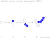 |
Fig. 2 Scheme representing the dust growth characterised as ballistic cluster-cluster aggregation. The agglomerates collide with a clone of each as marked with filled circles. The figure is adopted from Okuzumi et al. (2009). |
Following Takeuchi & Lin (2002), we assumed that the gas pressure scale height hg and the isothermal sound speed cs are simply defined by power laws associated with the scaling exponent q = −1/2: 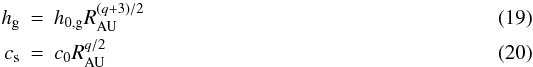 so that the gas density is defined by
 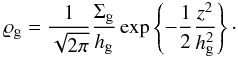 (21)Regarding the dust disc, we are primarily interested in conditions for which the mass flows associated with the settling and (vertical) turbulent mixing of the dust particles approach or attain a state of equilibrium. Taking the fast settling limit Ts/α ≫ (hg/R)2 into account, the dust density profile becomes
  cf. Takeuchi & Lin (2002). Approximating the settling time scale by tsed = (TSΩK)-1, we confirm in the fast settling limit the validity of
  (24)We considered that the gas is transparent to the emitted visible radiation of the protostar and neglected the contributions to the gas temperature from viscous dissipation. The temperature Tg of the gas is then given by
  (25)with T0 = 280 K (Hayashi 1981). Regarding the temperature of the dust particles, we drastically simplified the physics by setting Td = Tg, which is in line with previous studies (Sano et al. 2000; Bai & Goodman 2009). However, we are aware of the effect stellar radiation has on dust particles at high altitude (i.e., the so-called “superheated layer”) and its consequences for the interior gas temperature as demonstrated by Chiang & Goldreich (1997). Chiang & Goldreich report that the superheated dust layer may change with R; for their particular model of the minimum mass solar nebula, they showed that the location of the superheated layer changes from z/hg = 5 at R = 3 AU to z/hg = 4 at R = 100 AU. For altitudes z/hg ≤ 3 we considered, that the dust particles may be located some distance below the superheated layer.
3. Chemical model
We briefly recall the constituents of a chemical model: its components (or species), the chemical reactions that cause time-dependent changes in the abundances of species, and the underlying kinetic equation for each component.
Regarding the class of chemical species applied, we considered gas-phase species, grain species, and mantle species. The latter are species adsorbed onto the grain surface and associated with the counterparts of the neutral gas-phase species. Using this nomenclature, we differentiate between reactions that involve mantle species and those that do not. As we did in Ilgner & Nelson (2006a), we refer to the former as mantle chemistry and the latter as grain chemistry. We considered two different types for the topology of grain particles:
Type 1: the grain particles are regarded as dust agglomerates made by dust growth. For our particular model, we consider agglomerates associated with the BCCA model. The individual agglomerates are also assigned to different grain charges with j = Zmin,...,Zmax. Details are given in Sect. 3.2.
Type 2: the grain particles are now characterised as spherical dust grains of a radius a0. The individual grain particles are assigned to different grain charges with j = Zmin,...,Zmax. These models are discussed in Sect. 3.3.
For the chemical reaction network, we applied the generalised version of a simplified chemical network introduced in Ilgner & Nelson (2006a) who named this the “modified Oppenheimer-Dalgarno model”. It is a modification of the reaction scheme proposed by Oppenheimer & Dalgarno (1974) and was obtained by adding the grain and mantle chemistry. We now dropped the restriction |Zmin| = |Zmax| = 2 we made in Ilgner & Nelson (2006a) and allow Zmin and Zmax to become free of choice. A full list of the chemical reaction schemes applied is given in Table 1. To keep the terminology simple, we still refer to this model as the “modified Oppenheimer-Dalgarno model”.
We benefit from the fact that for our particular chemical model the numerical solution of the kinetic equations associated with the equilibrium state is accompanied by an analytical solution. The key idea needed to construct the analytical solution was taken from Okuzumi (2009), who succeeded to obtain an analytical solution for the network of Umebayshi-Nakano (1990). Our network, i.e. the modified Oppenheimer-Dalgarno model, and the more complex Umebayashi-Nakano network use of the same chemical key processes. However, they differ significantly in the way neutral gas-phase species may stick onto grains. To facilitate the comparison with the Umebayashi-Nakano network, we precede this section by comparing the modified Oppenheimer-Dalgarno with the Umebayashi-Nakano network. Both networks and the chemical models presented in this section are evaluated at disc midplane z/hg = 0 under minimum mass solar nebula conditions applying Eqs. (2), (19)–(21), and (25).
List of reactions considered for the modified Oppenheimer-Dalgarno network.
Except for the sticking coefficient se = 0.3, the ionisation rate and the elemental abundance of metals xM were taken from Sano et al. (2000) to facilitate the comparison with previous studies. In particular, xM = 7.97 × 10⁻⁵δ where δ denotes the assumed heavy metal gas depletion with respect to solar abundances. δ = 0.02 is regarded as the most favourable condition for retaining metals in the gas-phase. In Sect. 6 we follow a complementary approach by making a conservative estimate with xM ≪ 7.97 × 10⁻⁵δ.
3.1. Comparison: modified Oppenheimer-Dalgarno vs. Umebayashi-Nakano network
Both chemical networks are frequently applied, e.g., in studies on the dead zone structure of protoplanetary discs. In particular, under conditions typically applied for protoplanetary discs the ionisation degree and grain charging processes are closely related, cf. Ilgner & Nelson (2006a). Tracing the dead zone structure of protoplanetary discs, the chemical network associated with the modified Oppenheimer-Dalgarno model has been compared with more complex chemical networks, cf. Ilgner & Nelson (2006a) and Bai & Goodman (2009). While Ilgner & Nelson were concerned with conventional α-disc models, Bai and Goodman applied minimum mass solar nebula conditions. Considering a huge range of grain depletion, Bai and Goodman showed that the complex network generates more free electrons, which are less than ≲2 times the values obtained for the modified Oppenheimer-Dalgarno model.
Similar to Oppenheimer & Dalgarno (1974), the network of Umebayashi & Nakano (1990) was originally designed under dense interstellar cloud conditions. Sano et al. (2000) adopted the scheme of Umebayashi and Nakano (with some modifications) to estimate the size of the dead zone under minimum mass solar nebula conditions. Okuzumi (2009) modified the Umebayshi-Nakano network to account for grain charging processes on irregular porous dust agglomerates. Again, to keep the terminology simple, the chemical networks presented in Sano et al. (2000) and Okuzumi (2009) are referred to as the Umebayashi-Nakano model.
We recall that the modified Oppenheimer-Dalgarno model and Umebayashi-Nakano model are quite similar in the way they are constructed. Grain charges up to |Z| ≤ 3 are considered. The networks use the schematic components m, m + , M, and M + . The components M and M + represent a heavy metal atom and its ionized counterpart. The networks differ when specifying the molecular ion m + . In the modified Oppenheimer-Dalgarno model, m+ simply denotes the ion of the dominant molecule, while the ions  contribute to m + in the scheme of the Umebayashi-Nakano model. Umebayashi & Nakano introduced this extension because molecular ions react differentially. Only a few of the ions do react via charge transfer, others do not. In addition to the steady-state assumption for the neutral gas components
  , two chemical processes make the chemical networks different. The reaction scheme of the modified Oppenheimer-Dalgarno model includes the thermal adsorption of neutral gas-phase particles on grain surfaces and its corresponding reverse desorption process, the scheme of Umebayashi & Nakano does not. As Bai & Goodman (2009) pointed out, one can estimate the temperature range beyond the adsorption that dominates the desorption process, and vice versa. For heavy metal atoms M the corresponding temperature range is much more narrow. For gas temperatures below a critical value, the grains are very effective at sweeping up metal atoms. This was demonstrated by Ilgner & Nelson (2006a) when studying which effect this has on the size of the dead zone in conventional α-discs.
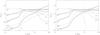 |
Fig. 3 Equilibrium concentrations at disc midplane shown for some representative components of the Umebayashi-Nakano (left panel) and the modified Oppenheimer-Dalgarno network (right panel), respectively. Apart from se = 0.3 the parameter setup is taken from Sano et al. (2000). The elements m and M of the modified Oppenheimer-Dalgarno network are specified by molecular hydrogen and magnesium. The line xi = ∞ at R = 10 AU is marked to aid comparison with the modified Oppenheimer-Dalgarno network applied to dust agglomerates, cf. Figs. 4–6. |
In a previous publication (Ilgner & Nelson 2006a) we have already examined the Umebayashi-Nakano network under minimum mass solar nebula conditions that reproduces the results of Sano et al. (2000). Varying se to 0.3, we have calculated the equilibrium abundances obtained for the modified Oppenheimer-Dalgarno and the Umebayashi-Nakano network, respectively. The profiles obtained for z/hg = 0 are shown in the left panel (Umebayashi-Nakano network) and in the right panel (modified Oppenheimer-Dalgarno network) of Fig. 3. The components m and M of the modified Oppenheimer-Dalgarno model are specified by molecular hydrogen and magnesium with evaporation energies of 450 K and 5300 K, respectively. We moreover assumed a standard value of 1.5 × 1015 cm-2 for the surface density of sites available on the grain surface. The comparison of the corresponding profiles revealed major changes in the metal ion M + abundance, which are remarkable, but not unexpected. According to Umebayashi & Nakano, M is steadily exchanging charges with the ionized molecules 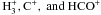 via charge transfer while keeping the reservoir of neutral metal atoms x∞ [M] constant and equal to the total fractional abundance of metals5. In the modified Oppenheimer-Dalgarno model at 135 K (R ~ 4.2 AU), the amount of metals adsorbed onto grain particles balances the gas-phase heavy metals. For lower temperatures essentially no metals are left in the gas phase and hence no metal atoms are available to be processed to metal ions via charge transfer reactions. Instead, the molecular ion m+ is becoming the dominant gas-phase ion for (R > 5 AU). However, the profiles for the ionisation fraction and the grain charges for the modified Oppenheimer-Dalgarno model and the Umebayashi-Nakano model agree very well.
We note that metals serve as the key ingredients in governing the chemistry in the original Oppenheimer-Dalgarno model as well as in the Umebayashi-Nakano model6. Comparing with the corresponding profiles obtained for the Umebayashi-Nakano network, we find that the amount of metal ions available is tremendously reduced in the modified Oppenheimer-Dalgarno network. Whether or not this may have significant consequences on the grain charging through reaction k7 listed in Table 1 will be analysed in the following subsection.
3.2. Grain chemistry with irregular porous agglomerates
The charging of irregular porous agglomerates was introduced by Okuzumi (2009), who applied the BCCA model to characterise the agglomerates. Okuzumi presented an analytical solution to obtain the equilibrium state of the ionisation degree and the excess charges Z of the dust agglomerates. The latter is well described by a Gaussian with a mean value of ⟨Z⟩ and a variance ⟨ΔZ2⟩, which is nicely detailed in Okuzumi (2009). However, at first glance the analytical solution might serve to verify the numerical solution rather than providing an a priori estimate. To recap: solving the corresponding equations (these are Eqs. (27)–(31) in Okuzumi 2009) requires knowing the final composition of the ions in order to calculate the mean ion velocity  and the mean gas-phase recombination rate
  . For a metal-rich environment, we have seen that the metal ion Mg + is by far the dominant ion in the Umebayashi-Nakano network (see previous subsection), which compensates its lower mean thermal velocity. We therefore simply set
  . As already mentioned in Okuzumi (2009), the contributions of
  are negligible for low values of the gas-phase recombination rate coeffcients applied.
With respect to the electrostatic polarisation of dust material caused by the electric field of an approaching charged particle, agglomerates and spherical particles differ significantly. Polarisation contributes to the mean collision rate coefficient  with
with  denoting the so-called “reduced rate” (Draine & Sutin 1987):
 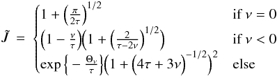 (26)with Θν ≈ ν/(1 + ν − 1/2). ν = Ze/qi relates the grain charge Ze to the charge of the colliding particle (q = e for singly charged ions and q = −e for electrons) while τ = akTq-2 refers to the so-called “reduced temperature”. In contrast to spherical dust particles, agglomerates are considered to be hardly affected by electrostatic polarisation, see discussion in Okuzumi (2009). For τ → ∞ and |ν| ≫ 1 the contributions to through polarisations become negligible and the expression for reduces to (Draine & Sutin 1987)
 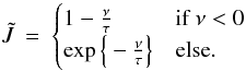 (27)The polarisation also effects the sticking coefficient se(a,Z,T), which is defined as
 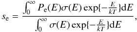 (28)assuming that the electron obeys a Maxwellian distribution at infinity. We also have to specify the grain topology since Pe depends on grain properties such as the grain surface. For example, Umebayashi & Nakano (1980) assumed planar surfaces to derive Pe. We did not investigate this question for dust agglomerates and simply assumed that se = 0.3 is independent of the grain charge. In particular, we regard se as an adjustable parameter of the simulations presented, which agrees with Okuzumi (2009).
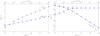 |
Fig. 4 Mean charge ⟨ Z ⟩ of dust agglomerates and the standard deviation |
When applying the formalism proposed by Okuzumi (2009) to the modified Oppenheimer-Dalgarno model, we followed a two step approach. To be able to compare our results with Fig. 3, we applied the same parameter setup. We began with switching off the adsorption and desorption process of the modified Oppenheimer-Dalgarno network, i.e., k5 = k6 = 0 (referring to Table 1), and ended in the analytical solution presented in Okuzumi (2009). The results obtained, for example at disc midplane at R = 10 AU, are shown in Fig. 4. The mean value ⟨ Z ⟩ and standard deviation of the excess charge Z of the dust agglomerate are shown in the left panel while the right panel reveals the outcome of the comparison between analytical and numerical values for the electron fraction x [e − ] , the molecule and metal ion concentration x [m + ] , x [M + ] , and the grain charge density approximated by ⟨ Z ⟩ xd. The analytical and numerical values agree excellently, which proves that our implementation of Okuzumi’s method is correct.
In a final step we constructed an analytical solution that covers k5k6 ≠ 0. The rates associated with thermal adsorption and desorption contribute exclusively to the rate equations of the neutral gas-phase components and the mantle components. The kinetic equations for the non-neutral gas-components remain unchanged and are (for t → ∞) ![\begin{eqnarray} N[\mathrm{m^+}] & = & k_4 N[\mathrm{m}] / \label{eq04:sec3} \\ & & \left( k_1 N[\mathrm{M}] + k_2 N_{\rm e} + v_{\mathrm{m^+}} n_d \langle \sigma[\mathrm{m^+}, N_d(Z)]\rangle \right) \nonumber \\ N[\mathrm{M^+}] & = & k_1 N[\mathrm{M}] N[\mathrm{m^+}] / \label{eq05:sec3} \\ & & \left( k_3 N_{\rm e} + v_{\mathrm{M^+}} n_d \langle \sigma[\mathrm{M^+}, N_d(Z)]\rangle \right) \nonumber \\ N_{\rm e} & = & k_4 N[\mathrm{m}] / \label{eq06:sec3} \\ & & \left( \beta N_{\rm i} + v_{\mathrm{e^-}} n_d \langle \sigma[\mathrm{e^-}, N_d(Z)]\rangle \right) \nonumber \\ \rm with & & \nonumber \\ n_d & = & \sum_Z N_d(Z) \nonumber \\ \beta N_{\rm i} & = & k_2 N[\mathrm{m^+}] + k_3 N[\mathrm{M^+}] \nonumber , \end{eqnarray}](/articles/aa/full_html/2012/02/aa18182-11/aa18182-11-eq218.png) where N [x] denotes the number density of the component x while Nd(Z) is the number density of grains with charge Z.
where N [x] denotes the number density of the component x while Nd(Z) is the number density of grains with charge Z.
However, the (thermal) adsorption/desorption of the neutral gas-phase components may have an indirect effect on both the ionized gas-phase species and the charge state of the dust since this process may control the amount of gas-phase species available. We will demonstrate that the set of Eqs. (29)–(31) and the charge balance equation  (32)can be solved for a single parameter ⟨ Z ⟩ if N [m] and N [M] serve as constants. Indeed, N [m] = const and N [M] = const can be extracted from the modified Oppenheimer-Dalgarno model. Molecular hydrogen serves as the neutral molecule component, which is assumed to relax towards hydrostatic equilibrium on a dynamical time scale
  (see Sect. 2.2). From the kinetic equation for the mantle component gM we obtained N [M] = k6NM/(k5nd + k6) assuming NM ≈ N [M] + N [gM] ; reaction k7 contributes to ⟨ Z ⟩ > 0 only. Solving the set of Eqs. (29)–(32), we obtained the semi-analytical solution for N∞ [m + ] , N∞ [M + ] , N∞ [e − ] , and ⟨ Z ⟩ ∞ (with N∞ denoting the asymptotic limit for t → ∞). The results obtained by numerical integration as well as by applying the semi-analytical approach are presented in Fig. 5. The agreement is excellent. We notice that the values associated with the “reduced” network of the modified Oppenheimer-Dalgarno model (i.e., with adsorption and desorption switched off k5 = k6 = 0) differ significantly from those of the “full network” with adsorption and desorption switched on (k5k6 ≠ 0). For N = const., the “reduced” network produces higher mean excess charges (associated with unlabelled red-coloured dotted lines in Fig. 5) than the same network does for k5k6 ≠ 0. The same applies for the electron concentration xe, ⟨ Z ⟩ xd and the ion concentration xi with m + becoming the dominant ion in the modified Oppenheimer-Dalgarno model.
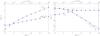 |
Fig. 5 Mean charge ⟨ Z ⟩ of dust agglomerates and the standard deviation |
Before we draw our conclusions, we investigate this problem for the Umebayashi-Nakano network, too. In particular, we analysed the effect of the dominant molecular ion HCO + on the grain charging under the assumption that the gas-phase metal is significantly depleted through the action of the thermal adsorption. We therefore have modified the Umebayashi-Nakano network by adding the thermal adsorption/desorption process for Mg7. The results obtained for calculations with rate coefficients k5 = k6 = 0 and k5k6 ≠ 0, respectively, are quite different compared with the results discussed above. Switching on the adsorption/desorption process for metals (i.e., k5k6 ≠ 0) leads to higher values for xe and xi and to higher negative mean charges on dust. However, the changes are just in the range of a few percent and therefore less severe than the changes observed in the modified Oppenheimer-Dalgarno network. These different features of the modified Oppenheimer-Dalgarno and the Umebayashi-Nakano network can be traced down to differences in the thermal velocity of dominant gas-phase ions. Under metal rich conditions, Mg + is the dominant ion in the modified Oppenheimer-Dalgarno network with k5 = k6 = 0, while  for k5k6 ≠ 0. Since has a much higher thermal velocity than Mg + it is quickly captured by grains. Applying the same conditions, HCO + becomes the dominant ion in the modified Umebayashi-Nakano network with a thermal velocity lower than that of Mg + , which is the dominant ion for k5 = k6 = 0. Because of the slightly reduced contributions owing to collisions between grains and HCO + , the values for xe and xi are increasing. The drop/rise in the mean grain charge observed in the modified Oppenheimer-Dalgarno and Umebayshi-Nakano model also originates in differences between the thermal velocities of the dominant gas-phase ions: the higher the thermal velocity of the dominant ion, the less the negative mean charge on grains. Considering all this, we find indeed that the adsorption/desorption of metals effects the mean value for grain charges, the electron fraction, and the ion abundances. Whether or not the value increases/decreases depends on the ratio of the thermal velocities for the metal ion and the dominant molecular ion.
3.3. Grain chemistry with spherical grains
Instead of agglomerates we now consider spherical dust grains of a given radius a0. Applying the modified Oppenheimer-Dalgarno model, we aim to determine their mean excess charge ⟨ Z ⟩ . If we neglect the effect of polarisation, ⟨ Z ⟩ can be calculated semi-analytically following the same procedure detailed in the previous subsection. We simply repeated the procedure and obtained an identical set of equations to Eqs. (29)–(32) by replacing  where Nd0(Z) and nd0 denote the number density of spherical grain particles with excess charge Z and the total number density of spherical grains, respectively. The results obtained are shown in Fig. 6. In the left panel the mean grain charge and its the standard deviation are plotted as a function of the grain radius, while the fractional abundances obtained are shown in the right panel. We first note the excellent agreement between the numerical and semi-analytical values. We can compare the results with those obtained for agglomerates when identifying the grain radius with a ∗ , see Eq. (18). Assuming monomers of size a0 = 10-5 cm, a ∗ scales with the number N of constituent monomers as shown in the upper x-axis of Fig. 6. A compact spherical dust grain of, for example, a ∗ = 10-3 cm corresponds to an agglomerate made by N = 106 monomers of size a0 = 10-5 cm. Comparing Fig. 5 with Fig. 6, we find that the mean charge carried by compact spheres is much lower than the value obtained for agglomerates. For N = 106, it is about one order of magnitude. This is not caused by the changes in the projected surface area associated with the transition between fractal and compact grain topology. It is because of the governing ion-electron regime in which the mean grain charge is proportional to the radius, i.e. ac/a ∗ = N1/6. For the same reason, the modified Oppenheimer-Dalgarno network applied to compact spherical grains produces a much larger amount of gas-phase ions m+ and e− and a much lower dust charge density ⟨ Z ⟩ xd than the values obtained for agglomerates. We conclude that dust agglomerates have a higher charge-to-mass ratio carrying more charges than the corresponding compact spheres.
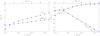 |
Fig. 6 Mean charge ⟨ Z ⟩ of spherical dust grains and the standard deviation |
We completed the cycle by taking the polarisation of compact spherical grains into account. We cannot apply the equations presented in Okuzumi (2009) though, which were derived under the assumption of Eq. (27). Substituting Eq. (27) with Eq. (26) leads to different expressions for ⟨ σdi ⟩ and ⟨ σde ⟩ . This may also affect the Gaussian distribution for Nd0(Z) since the coefficient W(Z) of the corresponding first-order equation changes (cf. Appendix in Okuzumi 2009). However, we did not consider the semi-analytical approach and performed a numerical integration of the rate equations taking Eq. (26) into account. The values for ⟨ Z ⟩ and ⟨ ΔZ2 ⟩ obtained under the assumption of Eq. (27) were used as an initial guess for the range of grain charges [Zmin,Zmax] considered. If necessary, the charge range was modified and the integration was repeated again until the calculated mean value ⟨ Z ⟩ fitted the peak value of the Gaussian profile for Nd0(Z). The values obtained by numerical integration match the analytical values associated with the non-polarised case very well. The corresponding profiles show no distinguishing features when applying the logarithmic scaling of Fig. 6. Changing to linear scales, we observe for sizes a < 10-4 cm that the analytical values (i.e. the model neglecting the polarisation) obtained for ⟨ Z ⟩ and ⟨ ΔZ2 ⟩ 1/2 are slightly lower than those obtained by numerical integration (model with polarisation). We conclude that at least for our particular disc model polarisation has only a minor effect on grain charging.
4. Ionisation rates
Because of the simplicity of the chemical network applied, all processes that might result in ionising disc material could not be treated individually. Instead, the contributions of the dominant processes were combined into an effective ionisation rate ζ with k4 = ζ (see Table 1).
We included the ionisation of the dominant molecule by incident X-rays that originate in the corona of the central T Tauri star. The corresponding X-ray ionisation rates ζxray can be obtained from radiative transfer calculations. The results of these calculations are presented in Igea & Glassgold (1999), who modelled the transport of stellar, low-energy X-rays ( < 20 keV). The ionisation rates are published primarily for the minimum solar nebula model of Hayashi et al. (1985), which corresponds to the static disc model discussed above. Taking the photoelectric absorption and Compton scattering into account, Igea & Glassgold specified absorption-dominated and scattering-dominated regimes, respectively. Bai & Goodman (2009) presented a best fit to the X-ray ionisation rates of Igea & Glassgold (1999), which facilitates employing the results of Igea & Glassgold (1999).
Igea & Glassgold (1999) presented ionisation rates obtained for power indices ps of the gas surface density Σg except for ps = −3/2. For a specified orbital radius at R = 1 AU they report that the deviation in the X-ray ionisation rate is generally less than a factor of two. Igea & Glassgold stated that the ionisation rates plotted vs. the vertical column density “manifest a universal form” that is independent of the surface density profiles considered. Glassgold et al. (2000) note that this “scaling is also found at other disk radii and is insensitive to changes in disk parameters such as disk mass, surface density, and slope q”8. However, X-ray ionisation rates obtained from X-ray transfer calculations have not been made publicly available yet for profiles of the gas surface density different from the static model of Hayashi et al. (1985).
Instead of a complex X-ray radiative transfer model, we attempted to apply a simple ray tracing model neglecting scattering effects. The techniques employed are described in detail in, e.g., Fromang et al. (2002) and Ilgner & Nelson (2006a). For static and stationary disc models of minimum mass solar nebula type, these calculations can be performed in straight line because of the non-discrete nature of the local gas density ϱg. We find significant differences when comparing the X-ray ionisation rates we obtained with the rates of Igea & Glassgold (1999). Similar findings are reported in Bai & Goodman (2009). The effect of scattering may explain these differences, but additional radiative transfer calculations would make valuable contributions.
Acknowledging the potential X-ray scattering may have on the ionisation rate, we applied X-ray ionisation rates based on the simulations of Igea & Glassgold (1999). In particular, we applied the fitting formula associated with Eq. (21) of Bai & Goodman (2009), which is valid for plasma temperature kBT = 3 keV. However, because of the problem discussed above we regard the X-ray ionisation rates ζXray as an order of magnitude estimate.
We also considered cosmic ray particles as a source for ionisation with ionisation rates ζCR given by Eq. (19) of Sano et al. (2000). We adopted the nominal value ζ0 = 10-17 s-1 of galactic cosmic rays associated with unattenuated penetration of cosmic ray particles. We neglected the minor contributions from the decay of radioactive elements. Taking the X-ray and the cosmic ray ionisation rates at face value, X-rays dominate the cosmic ray ionisation for regions close to the disc surface z/hg = 3. At higher optical depths, ionisation through cosmic rays is the dominant source of ionisation. We regard X-rays as our standard ionisation source while ionisation through cosmic rays is restricted to specific disc regions. For inner disc regions R < R1 we excluded cosmic rays and set ζ = ζXray. We furthermore assumed that the shielding effect of the T Tauri winds peters out between R1 < R < R2. We assumed a simple exponential decay 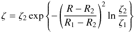 (33)to mimic this effect for that particular transition region from X-ray dominated to cosmic ray dominated regions with ζ1 = ζXray(R1,z) and ζ2 = ζCR(R2,z).
5. Numerical method
Although we applied a two-dimensional geometry (R,z), the dynamics of the gas-dust disc refers to a one-dimensional description. Therefore, no serious attempt was made to couple the dynamical and the chemical evolution of the gas-dust disc by means of conventional operator splitting techniques. The coupling is actually not required since the grain charging operates on a much shorter time scale than the disc dynamics. However, we aimed to simulate the disc dynamics to halt the simulation at different evolutionary stages. Assuming that the local disc structure is set up instantaneously, the kinetic equations are integrated numerically for t = 104 yr at each point of the two-dimensional domain. In parallel we determined the limiting behaviour (i.e., for t → ∞) following the semi-analytical approach.
In order to simulate the disc dynamics we continued by applying the so-called “method of line” (MOL) approach as we did, e.g., in Ilgner & Nelson (2006b), to solve the set of coupled advection-diffusion Eqs. (4) and (5). We applied a radial grid { Ri:i = 1,...,nR } with an equidistant mesh size near the inner boundary and non-equidistant mesh sizes elsewhere. The radial domain R = [0.1,103] AU was discretised using nR = 222 grid cells. The transport terms were discretised in the flux form to secure the conservation of mass. We applied the concept of staggered mesh on which the scalars and vectors representing the discrete values of the independent variables are centred at different locations. Scalars are located at zone centers while vectors are defined at zone edges. We limited the maximum absolute step size corresponding to a Courant-Friedrichs-Lewy (CFL) number of 0.5.
We applied the Crank-Nicholsen scheme when discretising the diffusion operator in Eq. (5), as we did in Ilgner & Nelson (2006b). Regarding the advection operator, we employed a nonlinear advection discretisation scheme that prevents negative values for the individual mass densities. In particular, we employed an upwind biased discretisation scheme with flux limiting. We opted for the flux limiter function proposed by Koren (1993), which – depending on the smoothness of the profile for the quantity to be advected – is associated with the accuracy of a third-order scheme.
The kinetic equations associated with the chemical model are given by a set of ordinary differential equations (ODE). We employed stiff ODE integrators to obtain stable numerical solutions. Stiffness was introduced for both physical and numerical reasons because of, e.g., the huge range of time scales for the chemistry and because of the semi-discretisation associated with the MOL approach. In particular, we used standard stiff ODE solvers based on linear multistep methods, namely the backward differentiation formulas.
Concerning the semi-analytic approach, we employed the procedure proposed by Muller (1956) to find the roots of the polynomial associated with Eqs. (29)–(32).
6. Results
In this section we present the results of simulations that examined the modified Oppenheimer-Dalgarno network under non-static disc conditions. We examined the modified Oppenheimer-Dalgarno network under stationary disc conditions which we later used for a comparison with the results obtained for non-stationary discs. We evolved the disc chemistry for t = 104 yr. However, by applying the semi-analytic approach discussed in Sect. 3, we are in the favourable position to calculate the long-term behaviour of the chemical models a priori. That is why we can prove the time interval needed to establish an equilibrium solution, which is (under the conditions applied) shorter than the dynamical time scale tK.
Apart from the radius a∗ and ac, respectively, we kept all other parameters fixed: M∗ = M⊙, μ = 2.33, α = 10-3, ϱp = 1.0 g cm-3, Sc = 1, h0,g = 3.33 × 10⁻² AU, and |Ṁd| = 10-10 M⊙ yr-1. We adopted values LX = 1029 erg s-1 and kBTX = 3 keV for the total X-ray luminosity and the plasma temperature while the transition between X-ray dominated and cosmic ray dominated ionisation region was fixed to R1 = 25 AU and R2 = 30 AU (see Sect. 4). The values for R1 and R2 were motivated by Perez-Becker & Chiang (2011), who discussed the problem of so-called “sideways cosmic rays”. Regarding the parameter setup associated with the chemical model we fixed the sticking coefficients se = 0.3 and si = 1.0, which is in line with the values Okuzumi (2009) applied. As we did in Ilgner & Nelson (2006a), we assumed the standard value of 1.5 × 1015 cm2 for the surface density of sites, while the value of energy ΔES transferred to the grain particle caused by lattice vibration was approximated by 2.0 × 10⁻³ eV. We approximated the dissociation energy D for neutral gas-phase components by its binding energy for physical adsorption. Complementary to the results discussed in Sect. 3, we applied a conservative estimate of xM = 10-11 in this section.
We are aware that the disc model we applied serves as a toy model and does not cover the complexity of the dust-gas dynamics. α = 10-3 is indeed a very naive approximation for the turbulence structure in discs and, in particular, in dead zones. However, recent simulations have shown that sound waves propagating into dead zones promote the diffusion of dust particles (Okuzumi & Hirose 2011). Lacking reliable models, we excluded grain size distributions. Instead we considered mono-sized particles and agglomerates and set limits on ac and a∗. We chose a∗ = [4.64 × 10-5,10-3] cm, which corresponds to agglomerates made of N = [102,106] monomers of size a0 = 10-5 cm. This limitation is motivated by recent studies of Okuzumi et al. (2011a,b). Evaluating a set of growth criteria for BCCA agglomerates, they made predictions on the location of so-called “frozen zones”. In frozen zones the electro-static barrier inhibits the agglomerates to growth further. The authors showed that planet forming regions
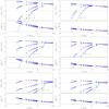 |
Fig. 7 Mean charge ⟨ Z ⟩ and the standard deviation |
are associated with frozen zones. The inferred sizes of the agglomerates are [4 × 10-5,3 × 10-2] cm, depending on the local position.
6.1. Stationary disc
The assumption of stationary discs, i.e., if the mass flow is constant with the orbital radius, corresponds to a gas surface density profile given in Eq. (8) with Σ0 = 350 g cm-2. One primary aim of this work is to determine to what extend compact spherical grains and dust agglomerates may allow for different grain charges Z. We already answered this question for a fixed dust-to-gas ratio Σd/Σg = 10-2 (see the preceding Sect. 3); in this section we conduct a similar exercise for a fixed mass flow of dust material Ṁd.
We already know that the population Nd(Z) (and Nd0(Z)) follows a Gaussian and therefore is completely characterised by the mean value ⟨ Z ⟩ and the variance ⟨ ΔZ2 ⟩ . In particular we compare compact spherical grains and dust agglomerates of the same mass, which constrains the radius a ∗ of the spherical grain. For BCCA agglomerates (with DBCCA = 2) relation Eq. (18) holds.
Figure 7 shows the result of the one-to-one comparison. In the left panel of Fig. 7 the mean value ⟨ Z ⟩ and the standard deviation  obtained for dust agglomerates at different altitudes are plotted against the orbital radius R. The agglomerates consist of N monomers of size a0 = 10-5 cm; the size of the agglomerate varies from N = 106 (top) to N = 102 (bottom) passing N = 104. The profiles of ⟨ Z ⟩ and obtained for the corresponding compact spherical grains are shown in the right panel with a∗ = 10-3 cm (top), a∗ = 2.15 × 10⁻⁴ cm (middle), and a∗ = 4.64 × 10⁻⁵ cm (bottom). While the solid and dotted lines refer to the values obtained by numerical integration, the values marked with (blue) filled circles correspond to the semi-analytical solution.
The first thing we comment on is the significant deviation of the analytical value of from the numerical value at disc midplane z/hg = 0 for R ≤ 1 AU. Each numerical value shown in Fig. 7 corresponds to the numerical solution of the ODE system for Δt = 104 yr. We confirmed by numerical integration that ⟨ ΔZ2 ⟩ approaches its equilibrium state beyond Δt = 104 yr because of the low ionisation rates in this particular region. For agglomerates with N = 106 we obtained, for example, at disc midplane at R = 0.7 AU  instead of
  . However, we also remark that because of ⟨ Z ⟩ → 0 − with decreasing R, the semi-analytical approach may fail to comply with the assumption Z < 0, which was made to construct the semi-analytical solution.
We found for the population of BCCA agglomerates that the grains follow the same population Nd(Z) for regions R > 30 AU independent of height z/hg. That is partly because cosmic ray particles become the dominant source of ionisation beyond R = 25 AU and therefore can penetrate easily towards disc midplane because of the low gas surface densities. However, we stress the more important matter of the ion-electron regime associated with these regions. Here Nd(Z) is determined by the grain size and the gas temperature, which is assumed to be independent of z.
Because TS ∝ a0, the three simulations presented in the left panel of Fig. 7 correspond to the same radial profile of Σd. We find that the mean value and the standard deviation decrease by reducing N and ⟨ Z ⟩ ∝ N for the ion-dust regime in particular (Okuzumi 2009). The profiles in the right panel of Fig. 7 show similar features.
In a next step we examined the population of BCCA agglomerates and compact spherical grains with respect to their excess charge. To recap: the populations Nd(Z) and Nd0(Z) are assumed to obey a Gaussian 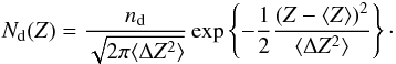 (34)Recalling the substantial changes in ⟨ Z ⟩ and (cf. Fig. 7), we expect significant changes with respect to their population. This is indeed what we observe in Fig. 8. There we plot the population Nd(Z) and Nd0(Z) (in terms of particle concentration) at disc midplane at R = 10 AU for BCCA agglomerates with N = 106 and compact spheres of a ∗ = 10-3 cm. Again, the solid lines refer to the values obtained by numerical integration while the values marked with (blue) filled circles correspond to the semi-analytical solution. Comparing with the corresponding profile for BCCA agglomerate, we find that for a given Ṁd i) the mean value obtained for spherical grains is shifted to lower values while ii) the distribution becomes much narrower. Differences regarding max [xd(Z)] are caused by small changes in Σd because of slightly different values for TS.
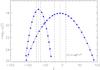 |
Fig. 8 Population Nd(Z) and Nd0(Z) (measured in particle concentration), respectively, vs. charge excess Z evaluated at disc midplane at R = 10 AU. The Gaussian distribution of Nd(Z)/ng with a peak around Z = −8 refers to agglomerates made of N = 106 monomers of size a0 = 10-5 cm while the profile with a peak at Z = −70 is obtained for compact spheres with a∗ = 10-3 cm. The dotted and the dashes lines mark ⟨ Z ⟩ and |

We compared the results obtained for BCCA agglomerates and the corresponding compact spheres
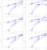 |
Fig. 9 Fractional abundances of the charge carrier associated with two different dust topologies as a function of the orbital radius R with |Ṁd| = 10-10 M∗ yr-1. The profiles shown in the left panel refer to BCCA agglomerates with N = 106 (top), N = 104 (middle), and N = 102 (bottom) monomers of a0 = 10-5 cm. The results obtained for the corresponding compact spheres are shown in the right panel. Here, the radius a∗ of the compact sphere varies from a∗ = 10-3 cm (top) to a∗ = 4.64 × 10⁻⁵ cm (bottom) passing a∗ = 2.15 × 10⁻⁴ cm. The lines correspond to the values obtained by numerical integration while the values marked by (blue) filled circles are obtained using the semi-analytical solution, see the discussion in the text. The (red-coloured) dashed lines refer to ⟨ Z ⟩ xd. |
with respect to the fractional abundances of the charge carrier xi, xe, and ⟨ Z ⟩ xd. The fractional abundances are shown in the left and right panels of Fig. 9, which correspond to those of Fig. 7. The values obtained by numerical integration and the semi-analytical solution (marked with (blue) filled circles) agree excellently. An important discriminant is given by xi ≈ xe separating the ion-electron plasma limit from the ion-dust plasma limit. The ion-dust plasma limit corresponds to xi ≫ xe. The results obtained for BCCA agglomerates indicate that the planet forming regions are always associated with the ion-dust regime. The profiles for xe, xi, and ⟨ Z ⟩ xd at disc midplane are also interesting. The profiles for N = 102 exactly fit those obtained for N = 104 and N = 106, and so does N = 104 and N = 106. The reason for this is simple since the cumulative projected surface area of all BCCA agglomerates is independent of N. The situation changes slightly when comparing the profiles obtained for compact spheres, as shown in the right panel of Fig. 9. Here, the transition from the ion-dust to the ion-electron regime becomes apparent in the profiles at z/hg = 2 in particular. The corresponding profiles at disc midplane also change systematically with increasing a∗.
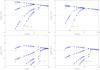 |
Fig. 10 Snapshots at t = 0 yr and t = 106 yr of dynamical disc evolution showing the mean charge ⟨ Z ⟩ associated with two different dust topologies as a function of the orbital radius R. The profiles shown in the left panel refer to BCCA agglomerates with N = 106 (top) and N = 102 (bottom) monomers of a0 = 10-5 cm. The results obtained for the corresponding compact spheres are shown in the right panel. Here, the radius a∗ of the compact sphere varies from a∗ = 10-3 cm (top) to a∗ = 4.64 × 10⁻⁵ cm (bottom). The dashed lines are associated with the profiles evaluated after t = 106 yr disc evolution; to aid comparison with the initial profiles we superimposed the corresponding profiles of Fig. 7 using dotted lines. As we did in the preceding figures, we mark the semi-analytical solution with (blue) filled circles. |
6.2. Non-stationary disc
We already analysed the grain charging i) under static disc conditions (see Sect. 3) and ii) under stationary disc conditions, see the preceding subsection. Comparing these with our results obtained under stationary disc conditions, we now explore the impact of the gas-dust dynamics on the grain charging. We recall the gas-dust dynamics that we analysed in Sect. 2: compact spherical grains with a∗ < 10-2 cm are tightly coupled to the gas because of TS ≪ 1. The turbulent mixing therefore dominates the advection of grains towards the central object. For dust particles treated as compact spheres we therefore expect that the evolving gas-dust disc dynamics causes minor changes in ⟨ Z ⟩ ,  , and the fractional abundances compared with the corresponding profiles obtained under stationary disc conditions. Regarding the BCCA agglomerates, we already know that the agglomerates with different N obey the same gas-dust disc dynamics. In particular, we find that the BCCA agglomerates are well coupled with the gas with no substantial inward migration (cf. right panel of Fig. 1). We conclude that the BCCA agglomerates considered (with N ≤ 106) and the corresponding compact spheres (with a∗ ≤ 10-3 cm) basically follow the similar dynamical evolution.
We repeated the simulations of Sect. 2 and let the gas-dust dynamics evolve. After t = 106 yr we stopped the calculation and examined the grain charging under local disc conditions. The profiles for ⟨ Z ⟩ are shown in Fig. 10 assuming BCCA agglomerates (left panel) and the corresponding compact spheres (right panel). In particular, we focused on grain charging of agglomerates made of N = 102 (bottom) and N = 106 (top) constituent monomers and the corresponding compact spheres of a∗ = 10-3 cm (top) and a∗ = 4.64 × 10⁻⁵ cm (bottom). We also compared the profiles obtained after t = 106 yr of dynamical evolution with the initial profiles at t = 0 yr (marked with dotted lines in Fig. 10). The results confirm our expectations demonstrating that the disc dynamics causes minor changes in the grain charging. However, we are aware that the situation may change if a more appropriate X-ray ionisation rate is taken, see discussion in Sect. 4.
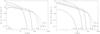 |
Fig. A.1 Radial profile of the surface densities of the gas and the dust particles at different time snaps t = 105,3 × 10⁵ and 106 yr with a0 = 1 mm and ϱp = 1.0 g cm-3. The parameter are α = 10-3 and Σd/Σg = 10-2 at t/tK = 0. The solid lines correspond to the dust surface density while the gas surface density is shown using the dashed lines. The dotted line refers to Σg ~ R-1 at t/tν = 0. The profiles shown in the left panel are obtained using the boundary conditions of Takeuchi & Lin (2005). Moving the inner boundary to smaller R and applying an analytical prescription for Σg at the inner and outer boundary cause the profiles to change as shown in the right panel. |
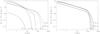 |
Fig. A.2 Radial profile of the surface densities of the gas and the dust at different time snaps t = 105,3 × 10⁵ and 106 yr. The solid lines correspond to the dust surface density while the gas surface density is shown using the dashed lines. The (red-coloured) dotted line refers to Σg ~ R-1 and Σd = Ṁd/(2πR ⟨ vR,d ⟩ ) at t/tK = 0. |Ṁd| = 10-10 M⊙/yr, α = 10-3, and ϱp = 1.0 g cm-3. The profiles shown in the left panel are obtained under the assumption of spherical grains with a0 = 1 mm. The corresponding profiles obtained for agglomerates with DBCCA = 2 and N = 1012 monomers of a0 = 10-5 cm are shown in the right panel. |
7. Summary
We have presented calculations of the grain charging under conditions that mimic different stages of protoplanetary disc evolution. Instead of parametrising the dust-to-gas ratio, we inferred the value for Σd(R)/Σg(R) from the evolution of the gas-dust disc. In particular, we applied the disc model of Takeuchi & Lin (2002, 2005) and content ourself with order-of-magnitude estimates. We considered collisional charging as the dominant process to determine the charge state of grains. For that purpose, we generalised the modified Oppenheimer-Dalgarno model introduced in Ilgner & Nelson (2006a) to account for higher grain charges. Based on that simple chemical network, we examined the grain charging for two different types of grain topology: compact spherical grains and fractal agglomerates of Df = 2. Our main conclusions are:
-
1.
The effect that thermal adsorption/desorption of metals has ongrain charging depends on the mass of the dominant moleculargas-phase ion. If its mass is heavier than that of metal, theinclusion of the thermal adsorption of metals results in highnegative excess charges on grains on average. Less negativecharge excess on average is observed for molecular ions lighterthan metals.
-
2.
We extended the semi-analytical method proposed by Okuzumi (2009), which allowed us to determine steady-state solutions for the mean grain charge, electron and ion abundances associated with the modified Oppenheimer-Dalgarno model. The semi-analytical solutions were derived for both grain topologies: compact grains and fractal aggregates.
-
3.
The results obtained confirm that dust agglomerates have a higher charge-to-mass ratio than the corresponding compact spheres.
-
4.
We found that reducing the number N of constituent monomers causes a drop in the mean value ⟨ Z ⟩ of the grain charge and the standard deviation
. Under conditions valid for the ion-dust plasma limit (i.e., xi ≫ xe) the profiles for ⟨ Z ⟩ xd, xe, and xi remain unchanged with varying N. This is because the cumulative projected surface area of all BCCA agglomerates is independent of N. -
5.
The results obtained by switching from one type of grain topology (fractal agglomerates) to another (compact spheres) reveal that for compact spherical grains ⟨ Z ⟩ is shifted towards more negative values while
decreases. -
6.
The results obtained for agglomerate sizes ac = [10-4,10-2] cm indicate that the grain charging of BCCA agglomerates is governed by the ion-dust plasma limit. Transitions from the ion-dust to the ion-electron plasma limit are observed for compact spheres depending on altitude z/hg.
-
7.
Another conclusion is that grain charging in a non-stationary disc environment is expected to lead to similar results as long as the effective ionisation rate and the temperature of the gas match the stationary values.
We regard the drastically simplified description of the temperatures of the gas and the dust mentioned above as a potentially serious omission of our model. Working out more realistic conditions may result in significant changes in the local disc structure and might be a potential problem for future investigations.
The characteristic radius ac serves to measure the size of the agglomerate. In particular, its weighting is different from the rms-definition of the gyration radius rg, cf. Okuzumi et al. (2009).
Problems related to the steady state assumption of neutral metal atoms are discussed for the original Oppenheimer-Dalgarno model in Ilgner & Nelson (2006a), where it was labelled model1.
Under certain conditions, this may have important consequences for ongoing planet formation in discs: in the ion-electron plasma limit (see Sect. 6.1) the structure of the dead zone may be significantly altered by the combined action of recombination of metal ions and turbulent transport (Ilgner & Nelson 2006b, 2008).
In Glassgold et al. (2000) q refers to the power index associated with the radial variation of the gas density.
Acknowledgments
I appreciate the discussions with Hiroshi Kobayashi, Satoshi Okuzumi, and Taku Takeuchi very much indeed.
References
- Bai, X.-N., & Goodman, J. 2009, ApJ, 701, 737 [NASA ADS] [CrossRef] [Google Scholar]
- Balbus, S., & Hawley, J. 1991, ApJ, 376, 214 [NASA ADS] [CrossRef] [Google Scholar]
- Chiang, E., & Goldreich, P. 1997, ApJ, 490, 368 [NASA ADS] [CrossRef] [Google Scholar]
- Desch, S. 2007, ApJ, 671, 878 [NASA ADS] [CrossRef] [Google Scholar]
- Draine, B., & Sutin, B. 1987, ApJ, 320, 803 [NASA ADS] [CrossRef] [Google Scholar]
- Epstein, P. 1923, Phys. Rev., 22, 710 [Google Scholar]
- Fleming, T., & Stone, J. 2003, ApJ, 585, 908 [NASA ADS] [CrossRef] [Google Scholar]
- Fromang, S., Terquem, C., & Balbus, S. 2002, MNRAS, 329, 18 [NASA ADS] [CrossRef] [Google Scholar]
- Glassgold, A., Feigelson, E., & Montmerle, T. 2000, Protostar and Planets V, ed. V. Mannings, A. P. Boss, & S. S. Russell, 429 [Google Scholar]
- Gressel, O., Nelson, R. P., & Turner, N. 2011, MNRAS, 415, 3291 [NASA ADS] [CrossRef] [Google Scholar]
- Hawley, J., & Balbus, S. 1991, ApJ, 376, 223 [NASA ADS] [CrossRef] [Google Scholar]
- Hayashi, C. 1981, Prog. Theor. Phys. Supp., 70, 35 [CrossRef] [Google Scholar]
- Hayashi, C., Nakazawa, K., & Nakagawa, Y. 1985, Protostar and Planets II, ed. D. C. Black & M. S. Mathews,, 1100 [Google Scholar]
- Hughes, A. M., Wilner, D., Andrews, S., Qi, C., & Hogerheijde, M. 2011, ApJ, 727, 85 [NASA ADS] [CrossRef] [Google Scholar]
- Igea, J., & Glassgold, A. 1999, ApJ, 518, 848 [NASA ADS] [CrossRef] [Google Scholar]
- Ilgner, M., & Nelson, R. P. 2006a, A&A, 445, 205 [NASA ADS] [CrossRef] [EDP Sciences] [Google Scholar]
- Ilgner, M., & Nelson, R. P. 2006b, A&A, 445, 223 [CrossRef] [EDP Sciences] [Google Scholar]
- Ilgner, M., & Nelson, R. P. 2008, A&A, 483, 815 [NASA ADS] [CrossRef] [EDP Sciences] [Google Scholar]
- Koren, B. 1993, Notes Numer. Fluid. Mech., 45, 353 [Google Scholar]
- Lynden-Bell, D., & Pringle, J. 1974, MNRAS, 168, 603 [NASA ADS] [CrossRef] [Google Scholar]
- Meakin, P. 1997, Rev. Geophys., 29, 317 [Google Scholar]
- Minato, T., Köhler, M., Kimura, H., Mann, I., & Yamamoto, T. 2006, A&A, 452, 701 [NASA ADS] [CrossRef] [EDP Sciences] [Google Scholar]
- Muller, D. E. 1956, Math. Tables Aids Comp., 10, 208 [Google Scholar]
- Okuzumi, S. 2009, ApJ, 698, 1122 [NASA ADS] [CrossRef] [Google Scholar]
- Okuzumi, S., & Hirose, S. 2011, ApJ, 742, 65 [NASA ADS] [CrossRef] [Google Scholar]
- Okuzumi, S., Tanaka, H., & Sakagami, M. 2009, ApJ, 707, 1247 [NASA ADS] [CrossRef] [Google Scholar]
- Okuzumi, S., Tanaka, H., Takeuchi, T., & Sakagami, M. 2011a, ApJ, 731, 95 [NASA ADS] [CrossRef] [Google Scholar]
- Okuzumi, S., Tanaka, H., Takeuchi, T., & Sakagami, M. 2011b, ApJ, 731, 96 [NASA ADS] [CrossRef] [Google Scholar]
- Oppenheimer, M., & Dalgarno, A. 1974, ApJ, 192, 29 [NASA ADS] [CrossRef] [Google Scholar]
- Perez-Becker, D., & Chiang, E. 2011, ApJ, 727, 2P [NASA ADS] [CrossRef] [Google Scholar]
- Pringle, J. 1981, A&ARv, 19, 137 [Google Scholar]
- Sano, T., Miyama, S., Umebayshi, T., & Nakano, T. 2000, ApJ, 543, 486 [NASA ADS] [CrossRef] [Google Scholar]
- Sicilia-Aguilar, A., Hartmann, L., Briceño, Muzerolle, J., & Calvet, N. 2004, AJ, 128, 805 [NASA ADS] [CrossRef] [Google Scholar]
- Takeuchi, T., & Lin, D. 2002, ApJ, 581, 1344 [NASA ADS] [CrossRef] [Google Scholar]
- Takeuchi, T., & Lin, D. 2005, ApJ, 623, 482 [NASA ADS] [CrossRef] [Google Scholar]
- Umebayashi, T., & Nakano, T. 1980, Publ. Astron. Soc. Japan, 32, 405 [Google Scholar]
- Umebayashi, T., & Nakano, T. 1990, MNRAS, 243, 103 [NASA ADS] [CrossRef] [Google Scholar]
Appendix A: Initial-boundary-value problems concerning the gas-dust dynamics
We adopted the disc model of Takeuchi & Lin (2005) to simulate the dynamics of the gas-dust disc. The corresponding set of coupled partial differential Eqs. (4) and (5) are subjected to initial and boundary conditions. We already know that for different sets of the dust parameters (a,ϱp) the dynamics of the dust disc remains unchanged if the parameter sets correspond to the same stopping time TS. Takeuchi & Lin (2005) have introduced a non-dimensional parameter A to retain the same dust evolution for different values of the initial gas mass. In the Appendix we study the effect of the boundary conditions and the initial profile for Σd on the dynamics of the gas-dust disc adopting the fiducial model of Takeuchi & Lin (2005).
We therefore solved Eqs. (4) and (5) for dust sizes of a0 = 1 mm assuming Σg ∝ R-1 for t = t0 while Σd/Σg = 10-2 is truncated at R = 100 AU. Concerning the boundary conditions for Σg and Σd, Takeuchi and Lin applied zero torque boundary conditions at Rinner = 5/6 AU and Router = 103 AU. The profiles we obtained are shown in the left panel of Fig. A.1, which should be compared with the upper panel of Fig. 4 of Takeuchi & Lin (2005). They correspond very well. However, we briefly recall the initial profile for the gas surface density, which is marked in Fig. A.1 using (red-coloured) dotted lines. It represents the steady-state solution Σg ∝ R-1 discussed in Sect. 2.1, which was obtained under the assumption νt ∝ R. Applying the same power law νt ∝ R, Lynden-Bell & Pringle (1974) presented a similarity solution of Eq. (4) with dimensionless variables X = R/R0 and τ = t/t0 + 1. In the limit of X ≪ 1 the expression reduces to Σg ∝ X-1. At this point, the temporal change of the gas surface density shown in the left panel of Fig. A.1 becomes important. In particular, the positive gradients in the gas surface density at R ≤ 2 AU clearly indicate an inner boundary problem associated with the zero torque boundary conditions applied at R = 5/6 AU.
In order to mimic the dynamics of the gas-dust disc at the very inner disc regions more precisely, we set the inner boundary at Rinner = 0.1 AU. We also replaced the zero torque boundary conditions with predefined analytical values for Σg(t) applying the self-similarity solution given in Eq. (15). The most appropriate value for the constant a was applied to approximate Σg(t) in the outer disc regions. Applying the improved boundary conditions, we then repeated the simulation and obtained the profiles shown in the right panel of Fig. A.1. Comparing with the corresponding profiles in the left panel, we find that the time evolution of Σg at the outer disc regions remains unchanged while we observe Σg ∝ R-1 in the inner disc regions. The changes in Σd at late evolutionary stages are remarkable. While in Takeuchi & Lin (2005) the entire dust disc has vanished for t = 106 yr, the improved boundary conditions cause a significant slow-down the rapid accretion of mm-sized compact spherical grain particles onto the star.
We proceeded by reassessing the assumption Σd/Σg = const. at t = t0 that Takeuchi & Lin (2005) applied. We already mentioned the steady-state solutions (8) and (9). For small dust sizes a < 10-3 cm, Σd/Σg = const. corresponds very well to (8) and (9), for larger grains it does not. In stationary discs larger particles migrate inwards much faster, causing a size fractionation reported in Takeuchi & Lin (2002). Hence we repeated the calculation replacing the initial assumption Σd/Σg = const by |Ṁd| = const. For the sake of convenience we applied the value of Takeuchi & Lin (2002) Ṁd = 10-10 M⊙ yr-1, which is one order of magnitude lower than the corresponding mass flux of the gas Ṁg = 3πνΣg ~ 2.6 × 10⁻⁹ M⊙ yr-1. The results obtained are shown in the left panel of Fig. A.2. The initial profiles of Σd and Σg are shown using (red-coloured) dotted lines and confirm the size fractionation and Σd/Σg ≠ const at t = t0.
The grain particles are now regarded as BCCA agglomerates with a characteristic radius rc defined by Eq. (16). We can relate the single agglomerate made of N monomers of size a0 to a compact sphere of the same mass applying Eq. (18). According
to Eq. (18), a compact sphere of a ∗ = 10-1 cm corresponds to an agglomerate of N = 1012 monomers with a0 = 10-5 cm. The surface density profiles obtained for such a dust agglomerate are shown in the right panel of Fig. A.2. We observe that the dust is tightly coupled to the gas dynamics expanding because of turbulent mixing towards larger orbital radii R.
All Tables
All Figures
|
Fig. 1 Radial profile of the surface densities of the gas and the dust at different time snaps t = 105,3 × 10⁵ and 106 yr. The solid lines correspond to the dust surface density while the gas surface density is shown using the dashed lines. The (red-coloured) dotted line refers to Σg ~ R-1 and Σd = Ṁd/(2πR < vR,d > ) at t/tK = 0. |Ṁd| = 10-10 M⊙/yr, α = 10-3, and ϱp = 1.0 g cm-3. The profiles shown in the left panel are obtained under the assumption of spherical grains with a0 = 10-3 cm. The corresponding profiles obtained for agglomerates with DBCCA = 2 and N = 106 monomers of a0 = 10-5 cm are shown in the right panel. |
| In the text | |
|
Fig. 2 Scheme representing the dust growth characterised as ballistic cluster-cluster aggregation. The agglomerates collide with a clone of each as marked with filled circles. The figure is adopted from Okuzumi et al. (2009). |
| In the text | |
|
Fig. 3 Equilibrium concentrations at disc midplane shown for some representative components of the Umebayashi-Nakano (left panel) and the modified Oppenheimer-Dalgarno network (right panel), respectively. Apart from se = 0.3 the parameter setup is taken from Sano et al. (2000). The elements m and M of the modified Oppenheimer-Dalgarno network are specified by molecular hydrogen and magnesium. The line xi = ∞ at R = 10 AU is marked to aid comparison with the modified Oppenheimer-Dalgarno network applied to dust agglomerates, cf. Figs. 4–6. |
| In the text | |
|
Fig. 4 Mean charge ⟨ Z ⟩ of dust agglomerates and the standard deviation |
| In the text | |
|
Fig. 5 Mean charge ⟨ Z ⟩ of dust agglomerates and the standard deviation |
| In the text | |
|
Fig. 6 Mean charge ⟨ Z ⟩ of spherical dust grains and the standard deviation |
| In the text | |
|
Fig. 7 Mean charge ⟨ Z ⟩ and the standard deviation |
| In the text | |
|
Fig. 8 Population Nd(Z) and Nd0(Z) (measured in particle concentration), respectively, vs. charge excess Z evaluated at disc midplane at R = 10 AU. The Gaussian distribution of Nd(Z)/ng with a peak around Z = −8 refers to agglomerates made of N = 106 monomers of size a0 = 10-5 cm while the profile with a peak at Z = −70 is obtained for compact spheres with a∗ = 10-3 cm. The dotted and the dashes lines mark ⟨ Z ⟩ and |
| In the text | |
|
Fig. 9 Fractional abundances of the charge carrier associated with two different dust topologies as a function of the orbital radius R with |Ṁd| = 10-10 M∗ yr-1. The profiles shown in the left panel refer to BCCA agglomerates with N = 106 (top), N = 104 (middle), and N = 102 (bottom) monomers of a0 = 10-5 cm. The results obtained for the corresponding compact spheres are shown in the right panel. Here, the radius a∗ of the compact sphere varies from a∗ = 10-3 cm (top) to a∗ = 4.64 × 10⁻⁵ cm (bottom) passing a∗ = 2.15 × 10⁻⁴ cm. The lines correspond to the values obtained by numerical integration while the values marked by (blue) filled circles are obtained using the semi-analytical solution, see the discussion in the text. The (red-coloured) dashed lines refer to ⟨ Z ⟩ xd. |
| In the text | |
|
Fig. 10 Snapshots at t = 0 yr and t = 106 yr of dynamical disc evolution showing the mean charge ⟨ Z ⟩ associated with two different dust topologies as a function of the orbital radius R. The profiles shown in the left panel refer to BCCA agglomerates with N = 106 (top) and N = 102 (bottom) monomers of a0 = 10-5 cm. The results obtained for the corresponding compact spheres are shown in the right panel. Here, the radius a∗ of the compact sphere varies from a∗ = 10-3 cm (top) to a∗ = 4.64 × 10⁻⁵ cm (bottom). The dashed lines are associated with the profiles evaluated after t = 106 yr disc evolution; to aid comparison with the initial profiles we superimposed the corresponding profiles of Fig. 7 using dotted lines. As we did in the preceding figures, we mark the semi-analytical solution with (blue) filled circles. |
| In the text | |
|
Fig. A.1 Radial profile of the surface densities of the gas and the dust particles at different time snaps t = 105,3 × 10⁵ and 106 yr with a0 = 1 mm and ϱp = 1.0 g cm-3. The parameter are α = 10-3 and Σd/Σg = 10-2 at t/tK = 0. The solid lines correspond to the dust surface density while the gas surface density is shown using the dashed lines. The dotted line refers to Σg ~ R-1 at t/tν = 0. The profiles shown in the left panel are obtained using the boundary conditions of Takeuchi & Lin (2005). Moving the inner boundary to smaller R and applying an analytical prescription for Σg at the inner and outer boundary cause the profiles to change as shown in the right panel. |
| In the text | |
|
Fig. A.2 Radial profile of the surface densities of the gas and the dust at different time snaps t = 105,3 × 10⁵ and 106 yr. The solid lines correspond to the dust surface density while the gas surface density is shown using the dashed lines. The (red-coloured) dotted line refers to Σg ~ R-1 and Σd = Ṁd/(2πR ⟨ vR,d ⟩ ) at t/tK = 0. |Ṁd| = 10-10 M⊙/yr, α = 10-3, and ϱp = 1.0 g cm-3. The profiles shown in the left panel are obtained under the assumption of spherical grains with a0 = 1 mm. The corresponding profiles obtained for agglomerates with DBCCA = 2 and N = 1012 monomers of a0 = 10-5 cm are shown in the right panel. |
| In the text | |
Current usage metrics show cumulative count of Article Views (full-text article views including HTML views, PDF and ePub downloads, according to the available data) and Abstracts Views on Vision4Press platform.
Data correspond to usage on the plateform after 2015. The current usage metrics is available 48-96 hours after online publication and is updated daily on week days.
Initial download of the metrics may take a while.