| Issue |
A&A
Volume 538, February 2012
|
|
|---|---|---|
| Article Number | A45 | |
| Number of page(s) | 11 | |
| Section | Interstellar and circumstellar matter | |
| DOI | https://doi.org/10.1051/0004-6361/201118113 | |
| Published online | 31 January 2012 | |
The Herschel HIFI water line survey in the low-mass proto-stellar outflow L1448⋆
1
Osservatorio Astronomico di Roma, via di Frascati 33,
00040
Monteporzio Catone
Italy
e-mail: This email address is being protected from spambots. You need JavaScript enabled to view it.
2
Osservatorio Astrofisico di Arcetri, Largo Enrico Fermi
5, 50125
Florence,
Italy
3
Observatorio Astronómico Nacional (IGN),
Calle Alfonso XII 3,
28014
Madrid,
Spain
4
Department of Earth and Space Sciences, Chalmers University of
Technology, Onsala Space Observatory, 43992
Onsala,
Sweden
5
Leiden Observatory, Leiden University,
PO Box 9513, 2300 RA
Leiden, The
Netherlands
6
Max Planck Institut für Extraterrestrische Physik,
Giessenbachstrasse 1,
85748
Garching,
Germany
Received: 16 September 2011
Accepted: 24 November 2011
Abstract
Aims. As part of the WISH (Water In Star-forming regions with Herschel) key project, systematic observations of H2O transitions in young outflows are being carried out with the aim of understanding the role of water in shock chemistry and its physical and dynamical properties. We report on the observations of several ortho- and para-H2O lines performed with the HIFI instrument toward two bright shock spots (R4 and B2) along the outflow driven by the L1448 low-mass proto-stellar system, located in the Perseus cloud. These data are used to identify the physical conditions giving rise to the H2O emission and to infer any dependence on velocity.
Methods. We used a large velocity gradient (LVG) analysis to derive the main physical parameters of the emitting regions, namely n(H2), Tkin, N(H2O) and emitting-region size. We compared these with other main shock tracers, such as CO, SiO and H2 and with shock models available in the literature.
Results. These observations provide evidence that the observed water lines probe a warm (Tkin ~ 400−600 K) and very dense (n ~ 106−107 cm-3) gas that is not traced by other molecules, such as low-J CO and SiO, but is traced by mid-IR H2 emission. In particular, H2O shows strong differences with SiO in the excitation conditions and in the line profiles in the two observed shocked positions, pointing to chemical variations across the various velocity regimes and chemical evolution in the different shock spots. Physical and kinematical differences can be seen at the two shocked positions. At the R4 position, two velocity components with different excitation can be distinguished, of which the component at higher velocity (R4-HV) is less extended and less dense than the low velocity component (R4-LV). H2O column densities of about 2 × 10¹³ and 4 × 1014 cm-2 were derived for the R4-LV and the R4-HV components, respectively. The conditions inferred for the B2 position are similar to those of the R4-HV component, with H2O column density in the range 1014−5 × 1014 cm-2, corresponding to H2O/H2 abundances in the range 0.5−1 × 10⁻⁵. The observed line ratios and the derived physical conditions seem to be more consistent with excitation in a low-velocity J-type shock with strong compression rather than in a stationary C-shock, although none of these stationary models seems able to reproduce the whole characteristics of the observed emission.
Key words: stars: formation / stars: low-mass / ISM: jets and outflows / ISM: individual objects: L1448 / ISM: molecules
Herschel is an ESA space observatory with science instruments provided by European-led Principal Investigator consortia and with important participation from NASA.
© ESO, 2012
1. Introduction
Strong radiative interstellar shocks are produced by the interaction of supersonic mass ejections from young stellar objects with the dense ambient cloud. The observational signature of these shocks are the bright line emissions from molecules and atoms, whose excitation conditions and relative abundances reveal fundamental information on the type of interaction, and on the physical properties of both the jets and the ambient medium. In the dense environments of young proto-stars (the so-called Class 0 sources) the gas cooling occurs through emission of H2, CO and H2O over a wide range of wavelengths, spanning from near-IR to sub-mm wavelengths (e.g. Kaufman & Neufeld 1996; Flower & Pineau Des Forêts 2010). Among these main coolants of outflow shocks, water is the most sensitive to local conditions, since its abundance can vary by orders of magnitudes through the shock lifetime (e.g. Bergin et al. 1998). Owing to the difficulty of observing water with ground-based facilities, the study of water is restricted to IR/sub-mm telescopes from space. Dedicated sub-mm satellites, such as SWAS and Odin, have allowed for the first time to observe the ground-state ortho-H2O at 557 GHz and to compare its profile and abundance with that of CO (e.g. Franklin et al. 2008; Bjerkeli et al. 2009). The poor spatial resolution of these facilities together with the restriction of observing a single line have prevented the study of the water excitation conditions and their variations along outflows, however. Through the Infrared Space Observatory (ISO), on the other hand, it has been possible to infer the physical conditions of the warm component giving rise to strong water emission (e.g. Liseau et al. 1996; Giannini et al. 2001). Nonetheless, the limited spatial and spectral resolution have not allowed the association of this warm gas with a specific kinematical component. The Herschel Space Observatory is now able to overcome these limitations, thanks to its improved spatial and spectral resolution over a wide wavelength range.
As part of the WISH (Water In Star-forming regions with Herschel, van Dishoeck et al. 2011) key program, we are undertaking systematic observations of H2O transitions in young outflows, employing the two spectrometers onboard Herschel, HIFI and PACS. One of our main targets of investigation is the L1448-mm outflow. This flow, powered by a low-luminosity (11 L⊙) Class 0 proto-star located in Perseus (d = 235 pc, Hirota et al. 2011), is known to be a strong water emitter on the basis of ISO observations (Nisini et al. 1999, 2000). HIFI observations of water in the central region of the L1448 outflow (within 20′′ radius from the source) have been presented by Kristensen et al. (2011), who focused on the H2O properties in the extreme high-velocity gas associated with the source collimated jet.
In this paper, we present HIFI observations of several H2O transitions obtained in two active shocked regions along the L1448 flow. Our aim is to study the excitation conditions of H2O in the shocked gas, exploring, in particular, variations of excitation with velocity. We aim to study in this way the physical and chemical conditions of the interstellar medium, which has been affected by the shock.
2. Observations and data reduction
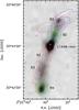 |
Fig. 1 PACS image of L1448 at 1670 GHz in false colors, with the negative contours in dotted line, and the JCMT CO(3−2) emission (Nisini et al., in prep.) in contours: the blue-shifted emission is integrated between –100 and 4 km s-1 and the red-shifted emission between 6 and 100 km s-1. The central position of the map and the positions chosen for the HIFI line survey (R4 and B2) are marked with a green cross. For the latter two positions the largest and the smallest HIFI beam sizes are shown in green. |
Summary of the HIFI line survey.
Figure 1 shows the JCMT CO(3−2) emission in contours overlaid on the PACS map of the H2O 212−101 emission at 1670 GHz toward L1448 (Nisini et al., in prep.). The H2O map exhibits several emission peaks, which correspond to positions of active shock regions, named B2-B3 (for the blue-shifted lobe) and R2-R3-R4 (for the red-shifted lobe), following the nomenclature of Bachiller et al. (1990), based on the analysis of CO line profiles. For our water line survey we selected the shock spots B2 and R4: the first corresponds to a bright H2 emission region (Davis & Smith 1995), arising from the interaction of the high-velocity jet from the mm source with the ambient medium; while the second is located at the end of the red-shifted lobe and is spatially associated with the bow-shock seen in SiO by Dutrey et al. (1997). Their offsets with respect to the central driving source L1448-mm (α(J2000) = 03h25m38 9, δ(J2000) = +30°44′05.′′4) are (−16′′, 34′′) for B2 and (26′′, −128′′) for R4, respectively.
A survey of several ortho- and para-H2O lines has been conducted with the HIFI heterodyne instrument (de Graauw et al. 2010) onboard the Herschel Space Observatory (Pilbratt et al. 2010) toward these two positions. The survey comprises lines with excitation energies ranging from 27 to 215 K and also includes the ortho- O 110−101 transition at 547.7 GHz, which is useful to infer opacity effects.
The data were processed with the ESA-supported package HIPE1 (Herschel interactive processing environment, Ott 2010) for calibration. The calibration uncertainty is taken to be 20%. Severe baseline problems were found at the B2 position in bands 6 and 4, corresponding to the ortho-H2O 212−101 line at 1670 GHz and the 312−303 line at 1097 GHz, respectively. Using the experimental “matching technique”2 for electronic standing waves, we obtained a tentative detection for the former line at a ~3σ level, which is consistent with the PACS map at 1670 GHz, presented in Fig. 1; for the latter only an upper limit was derived.
Further reduction of all spectra, including baseline subtraction, and the analysis of the data were performed using the GILDAS3 software. H- and V-polarizations were co-added after inspection; no significant differences were found between the two data sets. The calibrated  scale from the telescope was converted into the Tmb scale using the main-beam efficiency factors provided by Roelfsema et al. (2012)4, which are reported in Table 1. The beam sizes range from ~13′′ to 39′′. The largest and the smallest beam sizes of the HIFI observations are marked as green circles in Fig. 1, for each observed position. At the velocity resolution of 1 km s-1, the rms noise range is 3–100 mK (Tmb scale).
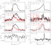 |
Fig. 2 HIFI spectra at the R4 (left) and B2 (right) positions. Note the different profiles for low-lying (black) and high-lying (red) levels at the R4 position. |
Transitions from other molecules were also observed in the HIFI bands centered on the water lines, namely NH3(10−00), 13CO(10−9), HCO+(6−5) and C18O(5−4). The only detected line among these is the NH3 transition at the B2 position, while for all the other transitions we have non-detections at a rms noise level (at the velocity resolution of 1 km s-1) of 4 mK (HCO+ 6−5 and C18O 5−4) and 20−26 mK (13CO 10−9). A summary of the observations, including frequencies (ν), beam sizes (HPBW), main-beam efficiencies (ηmb) and velocity-integrated intensities is given in Table 1.
3. Line profiles
The spectra of the H2O lines observed at the R4 and B2 spots are presented in Fig. 2 in the left and right panels.
At the R4 position, the water line profiles reveal a broad emission extending up to about 50 km s-1 with respect to the systemic velocity. The overlay between water line profiles with different upper level energies shows that the lines having Eu < 137 K peak at velocities around 25 km s-1, while the lines with higher upper level energies peak at lower velocities (around 10 km s-1). The different profiles of lines at different excitation could in principle be caused by high self-absorptions in the low-velocity range of those lines connecting with the ground state. This could be caused by the presence of large columns of cold water along the line of sight. However, we do not think this is the case, since the effect is not observed in the spectra obtained at the B2 position. In addition, as we will show below in Fig. 3, the profile of the H2O 110−101 line at 557 GHz matches the SiO J = 2−1 line profile well, which does not show any evidence of self-absorption even at the systemic velocity. The two velocity regimes at R4 (and correspondingly the different excitation lines) are therefore probably tracing gas with different physical conditions.
In particular, from the comparison of the shape of the profiles shown in Fig. 2, it can be noted that the lines at higher excitation (namely the o-H2O at 1097 GHz and the p-H2O at 752 GHz) have a simple triangular profile that peaks at low velocity, similar to those observed also in B2, while the other lines present an additional component that peaks at higher velocity, overlaid on the low-velocity triangular profile. It therefore seems that the observed profiles result from the superposition along the line of sight of two gas components, which have different kinematical and excitation properties.
Finally, the non-detection of the ortho-O 110−101 line at 548 GHz is shown in the bottom-left panel of Fig. 2, with an rms noise of about 3 mK (Tmb scale) at 1 km s-1 velocity resolution. This gives a constraint on the H2O 110−101 optical depth. Assuming an oxygen isotope ratio 16O/18O ~ 560 from Wilson & Rood (1994, for local interstellar medium) and under the assumption that the two lines have the same Tex, we find that τ557GHz < 15 at the peak of the H2O emission (based on O 3σ upper limit).
In contrast with R4, all detected lines at the B2 position show a similar triangular line profile with a line wing extending up to about −50 km s-1. Interestingly, among the detected H2O lines the highest excitation line (211–202 with Eu = 137 K) seems to show emission extending at high velocity, around −45 km s-1, at a level of 3σ. This may indicate the presence of high-excitation gas at high velocity.
The bottom-right panel of Fig. 2 also shows the NH3(10−00) emission line detected at B2. Ammonia emission is confined at the systemic velocity of about 5 km s-1, testifying to its origin from the molecular cloud and not from the outflow (see also Bachiller et al. 1990).
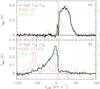 |
Fig. 3 Overlay between the HIFI H2O 557 GHZ line (black), IRAM-30 m SiO(2−1) line (red) from Nisini et al. (2007) and JCMT CO(3−2) line (green) from Nisini et al. (in prep.), toward the R4 (upper) and the B2 (lower) positions. |
Figure 3 shows the comparison between the H2O 110−101 line profile in black and that of SiO v = 0, J = 2−1 in red and the CO(3−2) in green (Nisini et al. 2007, 2011), toward both investigated positions. The figure highlights the very different line profile behavior at the two positions. In particular, the profile of the H2O line at 557 GHz follows the SiO profile at the R4 position quite closely, while at the B2 position the SiO emission is enhanced at the extreme high velocities (EHVs, v ~ 55 km s-1). Conversely, there is no water enhancement above the wing profile at the highest velocities, which suggests that the water emission from the EHV gas is observed only closer to the driving source (see also Kristensen et al. 2011; Nisini et al., in prep.). We discuss the different behavior of H2O and SiO line profiles at the two observed positions below in Sect. 5.
At both positions, the comparison with the CO(3−2) emission points out that H2O always has excess emission with respect to CO at intermediate velocities, suggesting that H2O and CO could trace different gas components. This will be discussed in Sect. 5 in more detail.
4. Excitation analysis
The physical conditions of the observed emitting regions were investigated by comparing the observed intensities with predictions from the RADEX escape probability code in plane-parallel geometry (van der Tak et al. 2007). Although the plane-parallel geometry is not able to reproduce the line profiles (e.g. Bjerkeli et al. 2011), it can be used as a first approximation for this study. The molecular data were taken from the Leiden Atomic and Molecular Database (LAMBDA5, Schöier et al. 2005), with the collisional rate coefficients from Faure et al. (2007).
As pointed out in Sect. 3, the profiles at the R4 position present two distinct components showing a clear change in excitation with velocity. We therefore need to separate the two velocity components and analyze them separately. An approach to separate the two velocity components in each line may be to fit the triangular component that peaks at low velocity in each water line and subtract it from the rest of the line. However, because fitting a triangular shape to the water lines is arbitrary, we opted for a simpler approach. We divided the emission at R4 into two velocity components: a low-velocity component (R4-LV hereafter, between 0 and 20 km s-1) and a high-velocity one (R4-HV hereafter, between 20 and 60 km s-1). As described in the appendix, the results of the analysis will be little affected by the method we used to separate the two velocity contributions, because both components dominate the relative velocity range we considered.
For B2, instead, we had too little information to perform an excitation analysis as a function of velocity, owing to the low signal-to-noise and the non-detection of one H2O line out of five, and therefore we integrated the emission over the whole velocity range. The observed velocity-integrated intensities for each component are given in Table 1.
We compared the integrated intensities with a grid of RADEX models, constructed by varying the parameters in the following ranges: n(H2) = 104−108 cm-3, N(ortho-H2O) = 1012−1016 cm-2, Tkin = 100−1600 K and ortho to para ratio o/p = 3,2.5,2,1.5. Line widths (FWZI) of 20, 40 and 50 km s-1 were adopted for R4-LV, R4-HV and B2, respectively. Given the different beam sizes of the observations, we also considered the size of the emission region (Θ) as an additional parameter: we varied it from almost point-like (few arcsec) to extended emission. A Gaussian emitting region and a Gaussian beam were assumed to correct the emitting size for beam dilution effects.
4.1. R4 position
The comparison of the observations with the RADEX grid of models shows that only a limited range of physical parameters is able to simultaneously reproduce both the line ratios and the line intensities in each component (see Figs. A.1 and A.2 in the appendix). In Fig. 4 these best-fit models are compared with the measured integrated intensities. For the R4-LV component, we are able to reproduce the observations within the calibration errors, assuming only extended warm gas (Tkin ~ 600 K) with a very high density n(H2) ~ 107 cm-3 (model LV-1 in Table 2). The implied column density is on the order of N(H2O) ~ 2 × 1013 cm-2, which indicates that the observed lines have low opacities (τ557GHz < 0.1), consistent with the non-detection of the O transition.
For the R4-HV component, on the other hand, the degeneracy in the physical parameters is higher (see Fig. A.2) and the observations can be reproduced either by 107 cm-3 gas at low temperature (Tkin ~ 150 K, model HV-1) or by gas as warm as in the R4-LV component, but with a lower density of ~106 cm-3 (model HV-2). It is therefore not possible at this stage to infer whether the lower excitation of the R4-HV component with respect to the R4-LV component, which is shown by the comparison of the line profiles, is caused by a temperature or a density effect. In both cases, the R4-HV component appears to be more compact (~13–21′′) and with a higher column density N(H2O) = (7−40) × 1013 cm-2, with respect to the R4-LV gas.
The different sizes found in the R4-LV and R4-HV components are consistent with the PACS map at 1670 GHz presented in Fig. 1. The map shows that the 1670 GHz emission at R4 is indeed dominated by a compact emission, which may correspond to R4-HV, superimposed on a more extended weak emission, which may correspond to R4-LV.
The physical conditions derived for the two components, in particular the very high density, can be compared with those inferred from other shock tracers, to see whether the observed H2O emission probes the same gas. Given the observed similarity between the H2O 557 GHz and the SiO(2−1) line profiles shown in Fig. 3, one would be tempted to conclude that the two species have similar excitation conditions. To test this hypothesis, we used the SiO multi-line observations at R4 presented by Nisini et al. (2007) to derive temperature and H2 density of the SiO gas in both the R4-LV and R4-HV components. We used a grid of LVG models, constructed from the RADEX code, and assumed an emission size on the order of 15′′ for both components, estimated from the IRAM Plateau de Bure (PdB) channel maps of the SiO(2−1) emission, presented by Dutrey et al. (1997).
Summary of the models derived for each component.
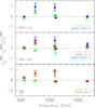 |
Fig. 4 Top and middle panels: comparison between the observed water intensities and the different models in Table 2, for R4-LV (top), R4-HV (middle) and B2 (bottom). The intensities predicted by the models have been corrected for the relative predicted filling factors. The given errors include 20% of calibration error. The triangles represent the models derived from H2O and the squares from the SiO. Bottom panel: same comparison as the top panels, but for B2. The upper limit of the non-detected H2O line at 1097 GHz is also shown for each model. |
The best-fit models that reproduce the SiO emission in the two velocity components are given in Table 2 (LVsio-2 for R4-LV and HVsio-3 and HVsio-4 for R4-HV). The models trace warm gas (Tkin between 250 and 600 K) but with H2 densities of only (1−5) × 104 cm-3, which is two orders of magnitudes lower than those derived from the H2O analysis. In particular, the H2 densities are lower than those derived from Nisini et al. (2007), n(H2) ≈ 2.5 × 105 cm-3 with T = 200 K, and this is probably caused by beam-filling effects that were not taken into account in Nisini et al. (2007). They assumed a beam-filling factor equal to 1, which implies that the line intensities are reproduced with a lower column density and consequently a higher particle density.
We then investigated how well the conditions estimated from the SiO emission reproduce the water lines, by varying the H2O column density to match the 557 GHz H2O line. The results are visualized in Fig. 4. For R4-LV, the SiO best-fit model underestimates the intensities of the water lines at higher excitation (para-H2O 211−202 at 752 GHz and ortho-H2O 312−303 at 1097 GHz). This could indicate that SiO is tracing an additional low-velocity gas component at lower excitation than that probed by H2O. Finally, for R4-HV we considered two possible SiO models (HVsio-3 and HVsio-4 in Table 2) and both of them reproduce only four out of the five H2O lines reasonably well.
The high-density regime found by the best-fit models, based only on the water lines, are more consistent with the conditions derived from Spitzer mid-IR H2 observations along the L1448 flow (Giannini et al. 2011). Although the R4 position is not covered by these observations, the other H2 shocked spots in the red-shifted lobe are consistent with a warm gas at densities on the order of 106 cm-3.
4.2. B2 position
At the B2 position we detect four (the 1670 GHz water line is only a tentative detection, however) out of the five targeted transitions: therefore we have too little information to constrain all parameters of the fit (see Fig. A.3 in the appendix). To overcome this problem, we assumed that the water emission originates from the same gas that emits the mid-IR H2 lines, which were observed with Spitzer (Giannini et al. 2011). This assumption is supported by the results found in other outflows observed within the WISH program (e.g. Nisini et al. 2010; Tafalla et al., in prep.). The H2 rotational transitions at low-J indicate a temperature of about 450 K, while a non-LTE fit through all the H2 lines suggests high densities in excess of 106 cm-3.
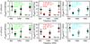 |
Fig. 5 Comparison between the observed line ratios (circles) of the H2O lines and the corresponding line ratios predicted (triangles) by the best-fit C-type shock (top) and the J-type shock (bottom) models. For each type of shock (C- and J-), the model that best reproduces our observed line ratios is presented and the corresponding shock velocity, pre-shock density and emission size are marked. The line ratios are normalized to the 1097 GHz line for R4-LV (left) and R4-HV (middle) and to the 1113 GHz line for B2 (right). For B2, the detected lines are shown as black filled circles, while the black open circle represents the upper limit of the non-detected H2O line at 1097 GHz (assuming a 3σ upper limit and a line width of 50 km s-1). |
Keeping these constraints, the fit is still degenerate in the product n(H2) × N(H2O), i.e. the data can be reproduced either by n(H2) ~ 6 × 106 cm-3 and N(H2O) = 1014 cm-2 (model B2-1 in Table 2 and Fig. 4) or n(H2) ~ 106 cm-3 and N(H2O) = 5 × 1014 cm-2 (model B2-2). The smaller size of the B2-2 model with respect to the B2-1 model seems to be consistent with the quite compact PACS emission at the B2 position, as shown in Fig. 1. Hence, the B2-2 model is indicated in Table 2 as the best model for the B2 component, even if it is associated with a poorer fit. Indeed, the comparison between the integrated intensities, predicted by the B2-2 model, as seen in Fig. 4, shows that the intensities of the H2O lines with the biggest beam sizes (at 557 GHz and 752 GHz) are slightly underestimated. This could be because the observations performed with these large beam sizes may collect emission from additional components, especially from the source position, as can be seen from the PACS map of Fig. 1.
5. Discussion
5.1. Water abundance
The presented excitation analysis shows that the observed HIFI water lines are consistent with warm gas at high density with moderate H2O column densities that do not exceed ~5 × 1014 cm-2. Similar water conditions have also been found in the L1157 flow (Vasta et al. 2012). These water column densities are significantly lower than those derived close to the L1448-mm source by Kristensen et al. (2011), who estimated N(H2O) 1016 cm-2 in all considered velocity components. This agrees with ISO observations of L1448 (Nisini et al. 1999, 2000), where the strongest water emission is found toward the central source. Moreover, this seems to suggest that the water emission from the EHV gas is only observed at high column densities, close to the driving source (see Kristensen et al. 2011), in contrast with other shock tracers.
H2O/CO abundance ratios found by Kristensen et al. (2011) are in the range 0.01–1, under the assumption that the two molecules are probing the same gas component. Adopting the same assumption, we applied the physical conditions derived from water to the CO(3−2) data and computed the corresponding CO column densities using the RADEX code. The data were corrected for beam dilution effects and the same sizes as estimated from water were assumed. The derived N(CO) values are high compared with water, ranging between ~5 × 10¹⁶ at R4-LV and HV, and 2 × 1017 cm-2 at B2. These values would imply a H2O/CO abundance ~10-4–10-2, if one assumes the typical CO/H2 ratio of 10-4, i.e. a water abundance extremely low for a shocked region. However, the assumption that the H2O and CO(3−2) emission come from the same region is likely not correct, given that they widely differ in both critical density (a factor of 103) and excitation temperature, and given also their different line profiles (Fig. 3). It is therefore conceivable that CO(3−2) traces mostly entrained ambient gas, while the H2O emission comes directly from the warm shocked gas.
A more direct estimate of the H2O abundance of the gas component traced by the HIFI lines can be obtained comparing the water column density with the H2 column density of the same component, inferred from Spitzer observations (Giannini et al. 2011; Dionatos et al. 2009). Only the B2 position was covered by these observations: the H2 gas is stratified in temperature, with the gas at T ~ 400–500 K having N(H2) on the order of 5 × 1019 cm-2 in a ~20′′ beam. The H2O abundance at B2, relative to this gas component, can therefore be constrained to be ~0.5−1 × 10⁻⁵. A similar abundance can be inferred for the R4-HV gas (whose estimated density is consistent with the average H2 density given by Giannini et al. 2011, along the flow), assuming that the same N(H2) applies to this component. This is clearly just a rough estimate, since we are comparing gas components at slightly different temperatures. These abundances are lower than those expected in non-dissociative, stationary shocks, where most of the gas-phase oxygen is converted into water (Kaufman & Neufeld 1996). The derived H2O abundances are higher than interstellar values, however, indicating that the observed warm gas has been processed by shock-related chemical processes.
5.2. Comparison with shock models
To better investigate the consistency of the observed emission with shock models, we compared the observed intensity ratios with the grid of stationary C- and J-type shocks provided by Flower & Pineau Des Forêts (2010). This grid explores different shock velocities (from 10 to 40 km s-1) and two pre-shock densities (2 × 10⁴ and 2 × 105 cm-3). For each type of shock (C- and J-), we have identified the model that better reproduces our observed line ratios. As for the RADEX analysis, the emission size was taken as an additional parameter, used to correct the intensity of lines with different beam sizes. The results are shown in Fig. 5, where the observed and predicted line ratios are plotted with respect to the 1097 GHz line for R4-LV and R4-HV and to the 1113 GHz line for B2. From the figure one can see that the line ratios at R4-HV are better reproduced by a J-type shock with a shock speed of 30 km s-1, consistent with the line width of this velocity component. The shock conditions of the R4-LV component are more degenerate: indeed, both shock models seem to reproduce the data within the uncertainties. There are different reasons to prefer the J-type shock model, however. First of all, the J-shock model has a shock speed of 20 km s-1 (versus 40 km s-1 for the C-shock), consistent with the line width of the R4-LV component. In addition, the best-fit J-shock model has a pre-shock density of 2 × 105 cm-3, higher than that predicted for R4-HV (2 × 104 cm-3), and this is consistent with our LVG analysis, showing that the difference in excitation between the R4-LV and R4-HV components can be caused by a different pre-shock density. The comparison between the post-shock density derived from the LVG analysis and the pre-shock density predicted by the J-shock indicates a compression factor npost/npre ~ 100, which is consistent with water emission originating from the post-shock gas regions farther behind the shock front, where H2, which has been initially dissociated, starts to reform, keeping the temperature to values around few hundreds of Kelvin (Flower & Pineau Des Forêts 2010).
At the B2 position, only the J-type shock predicts a shock velocity consistent with the observed wide line profiles (i.e. 30 km s-1 against 10 km s-1 for the C-type shock), although both C- and J-type shock models reproduce the line ratios. This best-fit J-type model predicts a shock speed of 30 km s-1 and a pre-shock density of 2 × 104 cm-3. Several additional lines of evidence indicate that a dissociative shock must be present at this position. Spitzer-IRS observations show that atomic emission from [Fe ii] 26 μm and [S i] 25 μm is associated with this position (Neufeld et al. 2009; Dionatos et al. 2009). PACS observations reveal emission from OH and [O i] 63 μm (Santangelo et al., in prep.): this is another indication that the gas-phase reactions that convert all the oxygen into water, activated at T300 K, have not been completed and dissociative shocks must be present to reach high OH emission (Neufeld & Dalgarno 1989).
There are also several inconsistencies between the considered models and our observations, however: in particular, none of these models (either C- or J-type) is able to reproduce the absolute intensities of the observed lines. Indeed, the comparison between the predicted and observed intensities would imply emission sizes much smaller (on the order of few arcsec) than those fitted through the line ratios. We believe that these discrepancies are due to the simplified nature of the adopted shock models. Indeed, a single, plane-parallel shock model is unlikely to provide a completely satisfactory representation of the line emission from a complex shock structure, where both geometrical and temporal effects can significantly alter the emerging line intensity and the final chemical abundance. In particular, several studies have shown that shocks from young outflows have not reached the steady state yet, and are consequently better represented with non-stationary shock conditions that combine both C- and J-type shock waves (Flower et al. 2003; Giannini et al. 2006; Gusdorf et al. 2008b). Predictions of H2O line intensities in CJ-shocks are provided for a limited set of conditions by Gusdorf et al. (2011): a qualitative comparison indicates that absolute intensities and water abundances derived in these models are similar to those observed in L1448. Clearly, the development of more specific models, suited for the shock regions under investigation, is needed for a better understanding of the water properties highlighted by our observations.
5.3. Comparison with SiO emission
Finally, we discuss the very different line profile behavior of H2O and SiO at the two investigated positions (see Fig. 3 in Sect. 3). At R4, the profile of the H2O line at 557 GHz follows the SiO profile quite closely. The SiO abundance is enhanced in shocks because of sputtering of silicon from the grain mantles, which is efficient at shock velocities as low as ~10 km s-1, and core grain disruption, which occurs at higher shock speeds on the order of 25−30 km s-1 (e.g. Jiménez-Serra et al. 2008; Gusdorf et al. 2008a). The observed SiO emission in both the R4-LV and R4-HV components is therefore consistent with the range of shock speeds we infer from the H2O analysis.
At B2, the comparison between water and SiO shows a more complex situation, with a strong variation of the SiO/H2O ratio as a function of velocity. This behavior probably reflects very different SiO/H2O abundance ratios in the various velocity regimes, indicative of a different chemistry rather than a difference in the excitation conditions. In particular, the SiO emission at B2 is enhanced at the EHVs (v ~ 55 km s-1), where no excess of water emission is detected. This is in contrast with the observations of water toward the driving source, where the EHVs water emission is clearly detected (Kristensen et al. 2011; Nisini et al., in prep.), which indicates that EHV water emission is more localized than SiO and shows up only in the regions with high water column densities. It has been suggested that the EHV gas traces the primary proto-stellar jet, where molecules are rapidly synthesized from the initial atomic gas (Tafalla et al. 2010). Available chemical models for the chemistry in the primary jet, although simplified in geometry and physical structure, predict a low H2O/SiO ratio for values of mass loss rates less than 10-5 M⊙ yr-1 (Glassgold et al. 1991), which agrees with the molecular mass flux rate of 10-7 M⊙ yr-1, derived for L1448-mm by Dionatos et al. (2009). Regarding the very low SiO associated with the wing emission, this is a bit puzzling given that these wings extend up to 50 km s-1, i.e. where one would expect sputtering to be very efficient in releasing silicon from grains. Tafalla et al. (2010), studying the chemistry of the L1448–R2 shock spot, which is located in the red-shifted lobe symmetrically to the B2 position, point out a strong trend of increasing SiO abundance with velocity, going from the lower velocities up to the EHV gas, which is not followed by the other molecules they observed. It therefore appears that there are strong chemistry variations across the various velocity regimes at different positions that are not easily explained by current shock chemical models.
6. Conclusions
Herschel observations of several ortho- and para-H2O transitions toward the outflow driven by the L1448 low-mass proto-stellar system have been presented. These observations are part of the WISH key program. Two shocked positions, R4 and B2, along the main L1448 outflow have been studied. The main results of this work are the following.
The two investigated positions (R4 and B2) show physical and chemical differences. In particular, R4 exhibits strong variations in the excitation conditions as a function of the LSR velocity and two velocity components can be distinguished in the water emission: a low-velocity component (R4-LV) and a high-velocity component (R4-HV). The excitation at R4 decreases with velocity, i.e. the lines with higher upper level energies peak at lower LSR velocity, while the lines with lower upper level energies peak at higher LSR velocity.
The observed emission in both shocked positions is best represented by very dense (nH2 ~ 106−107 cm-3) and warm (Tkin = 400−600 K) gas with moderate H2O column densities: N(H2O) ~ 1013 cm-2 at R4-LV and ~1014−5 × 1014 cm-2 at R4-HV and B2. These column density values correspond to H2O/H2 ~ 0.5−1 × 10⁻⁵ at B2 and R4-HV, obtained from comparison with N(H2) derived from Spitzer observations (Giannini et al. 2011).
The inferred physical conditions seem to be better reproduced by a J-type shock, where strong compression factors that lead to high density in the post-shock gas are expected. Moreover, the relatively low observed column densities and the PACS OH and [OI] 63 μm observations are consistent with models where H2O takes time to reform from fully dissociated gas. However, more detailed shock models are needed.
These Herschel H2O observations provide evidence that water is unique in tracing very dense shock components that are not traced by other molecules, such as CO and SiO, but rather traced by H2. In particular, H2O shows strong differences with SiO in the excitation conditions and in the line profiles in the two observed shocked positions, which points to chemical variations across the various velocity regimes at different positions.
HIPE is a joint development by the Herschel Science Ground Segment Consortium, consisting of ESA, the NASA Herschel Science Center, and the HIFI, PACS and SPIRE consortia.
The techniques are being developed at the HIFI ICC; see http://herschel.esac.esa.int/twiki/bin/view/Public/HifiCalibrationWeb?template=viewprint for references.
Acknowledgments
The authors are grateful to the WISH internal referees Sylvain Bontemps and Bengt Larsson for their constructive comments on the manuscript and to Paola Caselli for useful discussions. WISH activities in Osservatorio Astronomico di Roma are supported by the ASI project 01/005/11/0. B.N. and G.S. also acknowledge financial contribution from the agreement ASI-INAF I/009/10/0. HIFI has been designed and built by a consortium of institutes and university departments from across Europe, Canada and the United States under the leadership of SRON Netherlands Institute for Space Research, Groningen, The Netherlands and with major contributions from Germany, France and the US. Consortium members are: Canada: CSA, U. Waterloo; France: CESR, LAB, LERMA, IRAM; Germany: KOSMA, MPIfR, MPS; Ireland, NUI Maynooth; Italy: ASI, IFSI-INAF, Osservatorio Astrofisico di Arcetri- INAF; Netherlands: SRON, TUD; Poland: CAMK, CBK; Spain: Observatorio Astronómico Nacional (IGN), Centro de Astrobiología (CSIC-INTA). Sweden: Chalmers University of Technology – MC2, RSS & GARD; Onsala Space Observatory; Swedish National Space Board, Stockholm University – Stockholm Observatory; Switzerland: ETH Zurich, FHNW; USA: Caltech, JPL, NHSC.
References
- Bachiller, R., Martin-Pintado, J., Tafalla, M., Cernicharo, J., & Lazareff, B. 1990, A&A, 231, 174 [NASA ADS] [Google Scholar]
- Bachiller, R., Andre, P., & Cabrit, S. 1991, A&A, 241, L43 [NASA ADS] [Google Scholar]
- Bergin, E. A., Neufeld, D. A., & Melnick, G. J. 1998, ApJ, 499, 777 [NASA ADS] [CrossRef] [MathSciNet] [Google Scholar]
- Bjerkeli, P., Liseau, R., Olberg, M., et al. 2009, A&A, 507, 1455 [NASA ADS] [CrossRef] [EDP Sciences] [Google Scholar]
- Bjerkeli, P., Liseau, R., Nisini, B., et al. 2011, A&A, 533, A80 [NASA ADS] [CrossRef] [EDP Sciences] [Google Scholar]
- Davis, C. J., & Smith, M. D. 1995, ApJ, 443, L41 [NASA ADS] [CrossRef] [Google Scholar]
- de Graauw, T., Helmich, F. P., Phillips, T. G., et al. 2010, A&A, 518, L6 [NASA ADS] [CrossRef] [EDP Sciences] [Google Scholar]
- Dionatos, O., Nisini, B., Garcia Lopez, R., et al. 2009, ApJ, 692, 1 [NASA ADS] [CrossRef] [Google Scholar]
- Dutrey, A., Guilloteau, S., & Bachiller, R. 1997, A&A, 325, 758 [NASA ADS] [Google Scholar]
- Faure, A., Crimier, N., Ceccarelli, C., et al. 2007, A&A, 472, 1029 [NASA ADS] [CrossRef] [EDP Sciences] [Google Scholar]
- Flower, D. R., & Pineau Des Forêts, G. 2010, MNRAS, 406, 1745 [NASA ADS] [Google Scholar]
- Flower, D. R., Le Bourlot, J., Pineau des Forêts, G., & Cabrit, S. 2003, MNRAS, 341, 70 [NASA ADS] [CrossRef] [Google Scholar]
- Franklin, J., Snell, R. L., Kaufman, M. J., et al. 2008, ApJ, 674, 1015 [NASA ADS] [CrossRef] [Google Scholar]
- Giannini, T., Nisini, B., & Lorenzetti, D. 2001, ApJ, 555, 40 [NASA ADS] [CrossRef] [Google Scholar]
- Giannini, T., McCoey, C., Nisini, B., et al. 2006, A&A, 459, 821 [NASA ADS] [CrossRef] [EDP Sciences] [Google Scholar]
- Giannini, T., Nisini, B., Neufeld, D., et al. 2011, ApJ, 738, 80 [NASA ADS] [CrossRef] [Google Scholar]
- Glassgold, A. E., Mamon, G. A., & Huggins, P. J. 1991, ApJ, 373, 254 [NASA ADS] [CrossRef] [Google Scholar]
- Gusdorf, A., Cabrit, S., Flower, D. R., & Pineau Des Forêts, G. 2008a, A&A, 482, 809 [Google Scholar]
- Gusdorf, A., Pineau Des Forêts, G., Cabrit, S., & Flower, D. R. 2008b, A&A, 490, 695 [NASA ADS] [CrossRef] [EDP Sciences] [Google Scholar]
- Gusdorf, A., Giannini, T., Flower, D. R., et al. 2011, A&A, 532, A53 [Google Scholar]
- Hirota, T., Honma, M., Imai, H., et al. 2011, PASJ, 63, 1 [NASA ADS] [CrossRef] [Google Scholar]
- Jiménez-Serra, I., Caselli, P., Martín-Pintado, J., & Hartquist, T. W. 2008, A&A, 482, 549 [NASA ADS] [CrossRef] [EDP Sciences] [Google Scholar]
- Kaufman, M. J., & Neufeld, D. A. 1996, ApJ, 456, 611 [NASA ADS] [CrossRef] [Google Scholar]
- Kristensen, L. E., van Dishoeck, E. F., Tafalla, M., et al. 2011, A&A, 531, L1 [Google Scholar]
- Liseau, R., Ceccarelli, C., Larsson, B., et al. 1996, A&A, 315, L181 [NASA ADS] [Google Scholar]
- Neufeld, D. A., & Dalgarno, A. 1989, ApJ, 344, 251 [NASA ADS] [CrossRef] [Google Scholar]
- Neufeld, D. A., Nisimi, B., Giammini, T., et al. 2009, ApJ, 706, 170 [NASA ADS] [CrossRef] [Google Scholar]
- Nisini, B., Benedettini, M., Giammini, T., et al. 1999, A&A, 350, 529 [NASA ADS] [Google Scholar]
- Nisini, B., Benedettini, M., Giannini, T., et al. 2000, A&A, 360, 297 [NASA ADS] [Google Scholar]
- Nisini, B., Codella, C., Giannini, T., et al. 2007, A&A, 462, 163 [NASA ADS] [CrossRef] [EDP Sciences] [Google Scholar]
- Nisini, B., Benedettini, M., Codella, C., et al. 2010, A&A, 518, L120 [NASA ADS] [CrossRef] [EDP Sciences] [Google Scholar]
- Ott, S. 2010, Astronomical Data Analysis Software and Systems XIX, 434, 139 [NASA ADS] [Google Scholar]
- Pilbratt, G. L., Riedinger, J. R., Passvogel, T., et al. 2010, A&A, 518, L1 [CrossRef] [EDP Sciences] [Google Scholar]
- Roelfsema, P. R., Helmich, F. P., Teyssier, D., et al. 2012, A&A, 537, A17 [NASA ADS] [CrossRef] [EDP Sciences] [Google Scholar]
- Schöier, F. L., van der Tak, F. F. S., van Dishoeck, E. F., & Black, J. H. 2005, A&A, 432, 369 [NASA ADS] [CrossRef] [EDP Sciences] [Google Scholar]
- Tafalla, M., Santiago-García, J., Hacar, A., & Bachiller, R. 2010, A&A, 522, A91 [NASA ADS] [CrossRef] [EDP Sciences] [Google Scholar]
- van der Tak, F. F. S., Black, J. H., Schöier, F. L., Jansen, D. J., & van Dishoeck, E. F. 2007, A&A, 468, 627 [NASA ADS] [CrossRef] [EDP Sciences] [Google Scholar]
- van Dishoeck, E. F., Kristensen, L. E., Benz, A., et al. 2011, PASP, 123, 138 [NASA ADS] [CrossRef] [Google Scholar]
- Vasta, M., Codella, C., Lorenzani, A., et al. 2012, A&A, 537, A98 [NASA ADS] [CrossRef] [EDP Sciences] [Google Scholar]
- Wilson, T. L., & Rood, R. 1994, ARA&A, 32, 191 [NASA ADS] [CrossRef] [Google Scholar]
Appendix A: Diagnostic diagrams
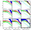 |
Fig. A.1 Diagnostic diagram to explore the parameter (Tkin, nH2, Northo−H2O, Θ) space that fits the observed data of the R4-LV component. The different panels are for three different values of the emission size (Θ = 5′′, 15′′ and 35′′) and three different temperatures (T = 150, 300 and 650 K). Three line ratios are reported in each panel: 557 GHz/1097 GHz (green), 1670 GHz/1097 GHz (blue) and 1113 GHz/1097 GHz (red); and the integrated intensity of the 1097 GHz line (cyan). An error of 10% is assumed for each line intensity. The thick boxes in this diagram and in all following diagrams mark the range of parameters for which all line ratios and line intensity intersect, corresponding to the physical conditions that are consistent with the observed data. |
The results of the excitation analysis presented in Sect. 4 are illustrated here with diagnostic plots that employ both line ratios and integrated intensities of the water lines. Each H2O emission component analyzed in the paper is shown separately: the two velocity components in the water emission from the R4 position, R4-LV and R4-HV, are shown in Figs. A.1 and A.2, respectively, while the water emission from the B2 position is presented in Fig. A.3.
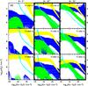 |
Fig. A.3 Diagnostic diagram to explore the parameter (Tkin, nH2, Northo−H2O, Θ) space for the water emission at the B2 position. The different panels are for three different values of the emission size (Θ = 5′′, 20′′ and 35′′) and three different temperatures (T = 150, 450 and 650 K). Three line ratios are reported in each panel: 557 GHz/1113 GHz (green), 1670 GHz/1113 GHz (blue) and 752 GHz/1113 GHz (yellow); and the integrated intensity of the 1113 GHz line (cyan). An error of 10% is assumed for each line intensity. |
In particular, we report a set of nine plots for each emission component to explore the parameter (Tkin, nH2, Northo−H2O, Θ) space and visualize the results given in Table 2 and Fig. 4. We considered the three most significant line ratios and one integrated line intensity. For the R4-LV and R4-HV components, the 557 GHz/1097 GHz (green), 1670 GHz/1097 GHz (blue) and 1113 GHz/1097 GHz (red) ratios and the integrated intensity of the 1097 GHz line are reported in each panel. For the B2 component, the 557 GHz/1113 GHz (green), 1670 GHz/1113 GHz (blue) and 752 GHz/1113 GHz (yellow) ratios and the integrated intensity of the 1113 GHz line are shown.
At R4, we divided the emission range of the water lines to separate the contribution from the two velocity components with different excitation conditions along the line of sight (R4-LV and R4-HV): between 0 and 20 km s-1 for the low-velocity component, R4-LV, and between 20 and 60 km s-1 for the high-velocity component, R4-HV.
As an example, Fig. A.1 for R4-LV shows that for a given temperature (T) and emission size (Θ) the line ratios only depend on the H2 density at low H2O column densities, without any dependence on the H2O column density; while for higher H2O column densities there is a degeneracy between the H2O column density and the H2 density, i.e. the line ratios depend on the product of both quantities. However, different line ratios and the integrated intensity of one line allow one to select only a limited region of the plane and therefore a limited range of physical conditions (i.e. in the case of R4-LV, all the line ratios and the integrated intensity of the selected line only intersect in the bottom-right panel of Fig. A.1).
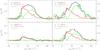 |
Fig. A.4 H2O line profile (black) decomposition in a triangular low-velocity component (red), derived by fitting the 752 GHz water line to the low-velocity emission profile, and a high-velocity component (green), obtained by subtracting the low-velocity component from the total water line profile. |
The following conclusions can be drawn from the inspection of the diagrams in Figs. A.1–A.3. The water emission at R4-LV is consistent with an extended component, with a very dense gas (higher than 107 cm-3) and low column density (a few 1013 cm-2). The temperature of this extended R4-LV component is high, about 600 K.
R4-HV, at lower excitation than R4-LV, can be reproduced by a less extended emission (about 15–20 arcsec) with a range of temperatures from 150 K to 650 K and either a higher density (higher than 107 cm-3) and lower column density (less than 1014 cm-2) or a lower density (around 106 cm-3) and higher column density (a few 1014 cm-2), respectively.
The emission at B2 appears to be consistent with an extended component (around 35 arcsec), with a wide range of temperatures, high density (higher than 106 cm-3) and low column density (around or lower than 1014 cm-2). However, we know from the PACS map at 1670 GHz toward L1448 (see Fig. 1) that the water emission comes from a more compact region. Therefore, the solution for an emission size about 20 arcsec was also considered, although it does not reproduce one of the line ratios (752 GHz/1113 GHz) for any of the displayed temperatures. Thus to additionally constrain the physical parameters of the water emission at the B2 position, some assumptions need to be made. As explained in Sect. 4, Spitzer mid-IR H2 observations from Giannini et al. (2011) were used in this context to constrain the temperature to ~450 K, assuming that water emission originates from the same gas that emits the mid-IR H2 lines.
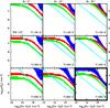 |
Fig. A.5 Diagnostic diagram to explore the parameter (Tkin, nH2, Northo−H2O, Θ) space for the water emission at R4-LV, after dividing the two velocity components as explained in the text and illustrated in Fig. A.4. The different panels are for three different values of the emission size (Θ = 5′′, 15′′ and 35′′) and three different temperatures (T = 150, 300 and 650 K). Three line ratios are reported in each panel: 557 GHz/1097 GHz (green), 1670 GHz/1097 GHz (blue) and 1113 GHz/1097 GHz (red); and the integrated intensity of the 1097 GHz line (cyan). An error of 10% is assumed for each line intensity to simplify the plots. |
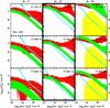 |
Fig. A.6 Same as Fig. A.5 for R4-HV. Two line ratios are reported in each panel: 557 GHz/1670 GHz (green) and 1113 GHz/1670 GHz (red); and the integrated intensity of the 1670 GHz line (cyan). Moreover, the upper limits to the 752 GHz/1670 GHz (yellow) line ratio is shown in the right panels, corresponding to Θ = 35′′. |
Finally, as mentioned in Sect. 4, we also explored how the derived results are affected by the method used to separate the high- and low-velocity components in R4. For that, we tried to deconvolve the line profiles into two different components based on the line shape: R4-LV being identified with the triangular profile seen especially in the higher excitation lines; while R4-HV corresponding to the high-velocity emission component that is overlaid on the triangular shape in the lower excitation water lines. Given the triangular line profile of the para-H2O 211−202 line at 752 GHz, we assumed that all emission in this line is coming from R4-LV. We therefore used this line as a template for separating the R4-LV contribution in each water line profile, as illustrated in Fig. A.4: we scaled the 752 GHz line to fit the low-velocity triangular contribution (red curve) in each water line profile (black curve) and then subtracted it from the rest of the line to obtain the R4-HV component (green curve). In this way we decomposed every water line profile into the two contributions from the R4-LV and R4-HV gas components. For each water line, both derived spectra have thus been integrated over the whole emission range to derive the integrated intensities of the two components.
We thus compared the derived line ratios and one integrated line intensity of R4-LV (Fig. A.5) and R4-HV (Fig. A.6) with the models. The considered integrated line intensities for each component are the 1097 GHz line for the R4-LV and the 1670 GHz line for R4-HV. Moreover, for R4-HV, we also show the upper limits to the 752GHz/1670GHz line ratio (yellow), derived from the 3σ upper limit of the 752GHz integrated intensity, in the only three panels where it is significant and can be used to distinguish between the different models.
The plots clearly highlight the same results as in the previous section, meaning that the approach we use to separate the two velocity components at different excitation at the R4 position does not affect the results of the analysis. This is mostly because the two velocity components are well separated in velocity (R4-LV peaks at about 10 km s-1 and R4-HV at about 25 km s-1) and therefore each of them dominates the water emission in the relative velocity range (0–20 km s-1 for R4-LV and 20–60 km s-1 for R4-HV) we chose in Sect. 4.
All Tables
All Figures
|
Fig. 1 PACS image of L1448 at 1670 GHz in false colors, with the negative contours in dotted line, and the JCMT CO(3−2) emission (Nisini et al., in prep.) in contours: the blue-shifted emission is integrated between –100 and 4 km s-1 and the red-shifted emission between 6 and 100 km s-1. The central position of the map and the positions chosen for the HIFI line survey (R4 and B2) are marked with a green cross. For the latter two positions the largest and the smallest HIFI beam sizes are shown in green. |
| In the text | |
|
Fig. 2 HIFI spectra at the R4 (left) and B2 (right) positions. Note the different profiles for low-lying (black) and high-lying (red) levels at the R4 position. |
| In the text | |
|
Fig. 3 Overlay between the HIFI H2O 557 GHZ line (black), IRAM-30 m SiO(2−1) line (red) from Nisini et al. (2007) and JCMT CO(3−2) line (green) from Nisini et al. (in prep.), toward the R4 (upper) and the B2 (lower) positions. |
| In the text | |
|
Fig. 4 Top and middle panels: comparison between the observed water intensities and the different models in Table 2, for R4-LV (top), R4-HV (middle) and B2 (bottom). The intensities predicted by the models have been corrected for the relative predicted filling factors. The given errors include 20% of calibration error. The triangles represent the models derived from H2O and the squares from the SiO. Bottom panel: same comparison as the top panels, but for B2. The upper limit of the non-detected H2O line at 1097 GHz is also shown for each model. |
| In the text | |
|
Fig. 5 Comparison between the observed line ratios (circles) of the H2O lines and the corresponding line ratios predicted (triangles) by the best-fit C-type shock (top) and the J-type shock (bottom) models. For each type of shock (C- and J-), the model that best reproduces our observed line ratios is presented and the corresponding shock velocity, pre-shock density and emission size are marked. The line ratios are normalized to the 1097 GHz line for R4-LV (left) and R4-HV (middle) and to the 1113 GHz line for B2 (right). For B2, the detected lines are shown as black filled circles, while the black open circle represents the upper limit of the non-detected H2O line at 1097 GHz (assuming a 3σ upper limit and a line width of 50 km s-1). |
| In the text | |
|
Fig. A.1 Diagnostic diagram to explore the parameter (Tkin, nH2, Northo−H2O, Θ) space that fits the observed data of the R4-LV component. The different panels are for three different values of the emission size (Θ = 5′′, 15′′ and 35′′) and three different temperatures (T = 150, 300 and 650 K). Three line ratios are reported in each panel: 557 GHz/1097 GHz (green), 1670 GHz/1097 GHz (blue) and 1113 GHz/1097 GHz (red); and the integrated intensity of the 1097 GHz line (cyan). An error of 10% is assumed for each line intensity. The thick boxes in this diagram and in all following diagrams mark the range of parameters for which all line ratios and line intensity intersect, corresponding to the physical conditions that are consistent with the observed data. |
| In the text | |
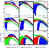 |
Fig. A.2 Same as Fig. A.1 for R4-HV. |
| In the text | |
|
Fig. A.3 Diagnostic diagram to explore the parameter (Tkin, nH2, Northo−H2O, Θ) space for the water emission at the B2 position. The different panels are for three different values of the emission size (Θ = 5′′, 20′′ and 35′′) and three different temperatures (T = 150, 450 and 650 K). Three line ratios are reported in each panel: 557 GHz/1113 GHz (green), 1670 GHz/1113 GHz (blue) and 752 GHz/1113 GHz (yellow); and the integrated intensity of the 1113 GHz line (cyan). An error of 10% is assumed for each line intensity. |
| In the text | |
|
Fig. A.4 H2O line profile (black) decomposition in a triangular low-velocity component (red), derived by fitting the 752 GHz water line to the low-velocity emission profile, and a high-velocity component (green), obtained by subtracting the low-velocity component from the total water line profile. |
| In the text | |
|
Fig. A.5 Diagnostic diagram to explore the parameter (Tkin, nH2, Northo−H2O, Θ) space for the water emission at R4-LV, after dividing the two velocity components as explained in the text and illustrated in Fig. A.4. The different panels are for three different values of the emission size (Θ = 5′′, 15′′ and 35′′) and three different temperatures (T = 150, 300 and 650 K). Three line ratios are reported in each panel: 557 GHz/1097 GHz (green), 1670 GHz/1097 GHz (blue) and 1113 GHz/1097 GHz (red); and the integrated intensity of the 1097 GHz line (cyan). An error of 10% is assumed for each line intensity to simplify the plots. |
| In the text | |
|
Fig. A.6 Same as Fig. A.5 for R4-HV. Two line ratios are reported in each panel: 557 GHz/1670 GHz (green) and 1113 GHz/1670 GHz (red); and the integrated intensity of the 1670 GHz line (cyan). Moreover, the upper limits to the 752 GHz/1670 GHz (yellow) line ratio is shown in the right panels, corresponding to Θ = 35′′. |
| In the text | |
Current usage metrics show cumulative count of Article Views (full-text article views including HTML views, PDF and ePub downloads, according to the available data) and Abstracts Views on Vision4Press platform.
Data correspond to usage on the plateform after 2015. The current usage metrics is available 48-96 hours after online publication and is updated daily on week days.
Initial download of the metrics may take a while.