| Issue |
A&A
Volume 536, December 2011
|
|
|---|---|---|
| Article Number | A33 | |
| Number of page(s) | 23 | |
| Section | Interstellar and circumstellar matter | |
| DOI | https://doi.org/10.1051/0004-6361/201117112 | |
| Published online | 05 December 2011 | |
Structure of the hot molecular core G10.47+0.03⋆
1
Max-Planck-Institut für Radioastronomie, Auf dem Hügel 69, 53121 Bonn, Germany
e-mail: This email address is being protected from spambots. You need JavaScript enabled to view it.
2
I. Physikalisches Institut, Universität zu Köln, Zülpicher Straße 77, 50937 Köln, Germany
e-mail: This email address is being protected from spambots. You need JavaScript enabled to view it.
3
Harvard-Smithsonian Center for Astrophysics, 60 Garden Street, Cambridge, MA 02138, USA
4
Centro de Radioastronomía y Astrofísica, UNAM, Apdo. Postal 3-72 (Xangari), 58089 Morelia, Michoacán, Mexico
Received: 20 April 2011
Accepted: 12 September 2011
Abstract
Context. The physical structure of hot molecular cores, where forming massive stars have heated up dense dust and gas, but have not yet ionized the molecules, poses a prominent challenge in the research of high-mass star formation and astrochemistry.
Aims. We aim at constraining the spatial distribution of density, temperature, velocity field, and chemical abundances in the hot molecular core G10.47+0.03.
Methods. With the SubMillimeter Array (SMA), we obtained high spatial and spectral resolution of a multitude of molecular lines at different frequencies, including at 690 GHz. At 345 GHz, our beam size is 0.3′′, corresponding to 3000 AU. We analyze the data using the three-dimensional dust and line radiative transfer code RADMC-3D for vibrationally excited HCN, and myXCLASS for line identification.
Results. We find hundreds of molecular lines from complex molecules and high excitations. Even vibrationally excited HC15N at 690 GHz is detected. The HCN abundance at high temperatures is very high, on the order of 10-5 relative to H2. Absorption against the dust continuum occurs in twelve transitions, whose shape implies an outflow along the line-of-sight. Outside the continuum peak, the line shapes are indicative of infall. Dust continuum and molecular line emission are resolved at 345/355 GHz, revealing central flattening and rapid radial falloff of the density outwards of 104 AU, best reproduced by a Plummer radial profile of the density. No fragmentation is detected, but modeling of the line shapes of vibrationally excited HCN suggests that the density is clumpy.
Conclusions. We conclude that G10.47+0.03 is characterized by beginning of feedback from massive stars, while infall is ongoing. High gas masses (hundreds of M⊙) are heated to high temperatures above 300 K, aided by diffusion of radiation in a high-column-density environment. The increased thermal, radiative, turbulent, and wind-driven pressure drives expansion in the central region and is very likely responsible for the central flattening of the density.
Key words: ISM: molecules / ISM: structure / ISM: clouds / stars: formation
Appendices A and B are available in electronic form at http://www.aanda.org
© ESO, 2011
1. Introduction
Massive stars and star clusters are born deeply embedded in molecular clouds (for a review, see Zinnecker & Yorke 2007). When cores have contracted enough to form massive stars, the dense dust and gas is heated by these stars. The ice mantles around dust grains evaporate, and a rich plethora of molecular lines can be observed, along with strong dust emission (Kurtz et al. 2000; Cesaroni 2005). Often, these hot molecular cores are associated with ultracompact or hypercompact Hii regions, which are ionized by newly formed massive stars (Hoare et al. 2007). The physical and chemical structure of hot molecular cores is very important for the study of high-mass star formation and of astrochemistry. Investigations of the structure are hampered, though, by the compactness of the sources, by their scarcity and large distance, and by the large foreground column density, which only long-wavelength radiation can pass.
What is needed, therefore, is high angular resolution at (sub)millimeter wavelengths, combined with high spectral resolution of many molecular lines, which contain all the information about chemistry, velocity field, and temperature. With the Submillimeter Array (SMA) in Hawaii, we observed the massive hot molecular core G10.47+0.03 at around 200, 345, and 690 GHz, yielding a best resolution of 0.3′′ and 350 identified molecular lines. Due to its high dust mass and high temperatures, this hot core is among the strongest sources at submillimeter wavelengths, although it is located at a distance of 10.6 kpc (Pandian et al. 2008). It has an estimated luminosity of 7 × 10⁵ L⊙ (Cesaroni et al. 2010) and displays exceptionally many lines from highly excited molecules (e.g. HC3N, Wyrowski et al. 1999).
Observational summary.
2. Observations and data reduction
The high-mass star-forming region G10.47+0.03 was observed with the Submillimeter Array1 (SMA) during five nights in different array and receiver configurations, yielding six two-GHz-wide bands centered at around 201, 211, 345, 355, 681, and 691 GHz. Table 1 summarizes the observations. We note that Jupiter was close (~10°) to the target source in 2008, so its moon Callisto could be used as gain calibrator at 690 GHz, where it is otherwise very difficult to find a suitable calibrator source. It was observed repeatedly for two minutes after spending ten minutes on the target source. For the 345 GHz observations in 2007 and 2009, after each 15 minutes we switched to 1733-130 (NRAO 530), which lies 10.9° away from the target source. In addition, strong sources (Uranus, Ceres, 3c454.3, 3c273) were observed before and after these loops to allow bandpass and flux calibration.
Calibration and editing of the data were done in the IDL MIR package2, involving correction and application of the system temperature, phase-only bandpass calibration, continuum regeneration (spectral averaging), phase-and-amplitude bandpass calibration, flagging, gain calibration (phase and amplitude), and flux calibration. The data were converted to MIRIAD3 (Sault et al. 1995), where the edge channels of each chunk were flagged and the channels were rebinned to a width of 1 km s-1 at 201 GHz, 0.75 km s-1 at 345 GHz, and 1.42 km s-1 at 681/691 GHz. Data from different dates were merged for each frequency setup. Since the 2007 observations had the phase center at RA 18:08:38.28, Dec –19:51:50.0, while the later observations were centered on RA 18:08:38.232, Dec –19:51:50.4, the 345/355 GHz data set had to be merged in AIPS. The channels that were less affected by spectral lines were identified and used for separating lines and continuum in MIRIAD. The continuum data of upper and lower sidebands were merged and imaged using almost uniform weighting at 201/211 GHz and 345/355 GHz (robust = −2) and more natural weighting at 681/691 GHz (robust = 0.5). A cutoff for cleaning of about three times the rms noise in the image was used. Based on these clean components, the continuum visibility data were self-calibrated, which substantially reduced the fluctuations outside the source, and the solutions were applied to the line data as well. Imaging of the spectrally resolved data was done with robust = 0.5 at 201/211 GHz and 345/355 GHz and robust = 2 at 681/691 GHz. Table 2 gives the resulting beam sizes and noise levels in the maps.
Beam sizes and noise levels.
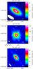 |
Fig. 1 Continuum maps of G10.47+0.03 observed with the SMA at 201/211 GHz (top panel), 345/355 GHz (central), and 681/691 GHz (bottom). The map size is either 5 or 10′′. Contours mark 20 and 50% of the peak flux, which is given in the lower right (in K). The beam is depicted in the lower left. The white crosses denote the Hii regions B1, B2, and A (Cesaroni et al. 2010, from left to right). |
Line identification was made with the myXCLASS program4, which accesses the CDMS5 (Müller et al. 2001, 2005) and JPL6 (Pickett et al. 1998) molecular data bases. The figures in this paper were produced with the GILDAS software7.
3. Observational results
3.1. Continuum
Figure 1 shows the obtained continuum maps. The total flux is 6 Jy at 201/211 GHz, 27 Jy at 345/355 GHz, and 95 Jy at 681/691 GHz, corresponding to a spectral index of 2.8 between the lower two and 1.8 between the upper two frequencies. While the beam sizes are not sufficient to resolve the continuum emission at 201/211 and 681/691 GHz, the extension can be clearly seen at 345/355 GHz. At this frequency, the peak intensity is 158 K (1.84 Jy/Beam), and the 3σ contour extends over 3′′.
3.2. Line identification
The data cubes were convolved to a common resolution of 5′′ and central spectra extracted. This resolution was chosen to decrease the noise and the effects of a strong continuum, as well as to facilitate a comparison between the different frequencies, and it gives the total (source-integrated) flux for most lines.
To identify the spectral features, a simple homogeneous model was computed in local thermodynamic equilibrium (LTE), using the myXCLASS program, which takes the different optical depths of the transitions into account. Synthetic spectra are compared to the data. A source size of 1.5′′ (half-maximum diameter of a Gaussian source), a temperature of 200 K, and a line width of 5 km s-1 were fixed, while the column density of each molecule was varied to obtain a good fit to the data (see Table 3). The continuum was neglected in the radiative transfer, and only a foreground absorbing column density of 5 × 1024 H2 cm-2 was considered to approximate the higher absorption at the higher frequencies (corresponding to τ = 0.3 at 345 GHz and τ = 1.3 at 690 GHz). Although this is only foreground absorption, it serves to account for both absorption and continuum emission, as the latter weakens the lines as well. Continuum levels of 6, 8, and 7 K were added to the spectra at 201/211, 345/355, and 681/691 GHz, respectively. Figures A.1 − A.3 show the spectra and the model, and Table 3 gives the derived column densities. We note that the model is not supposed to give an optimum fit to the data, but is just for identification purposes.
List of identified molecules.
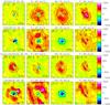 |
Fig. 2 Line maps (selected to trace expansion motions) integrated over the velocity range indicated in each panel (which can be considered, from left to right, as the high-velocity part of the outflow, low-velocity part, systemic velocity, and low-velocity part of the outflow at the far side). The first velocity range of HC3N is blended by other lines. In the second velocity range of CO the emission is extended this much to cause imaging artifacts. The map size is 5′′ (tick spaces are 1′′, centered on RA 18:08:38.236, Dec –19:51:50.25). Beams are shown in the lower left, and the number in the lower right of each panel is the maximum flux in K km s-1 (contours are ± 20 and 50% of that value). The color scale is from –1000 to 1000 K km s-1. The energy of the lower level is given in the upper left. |
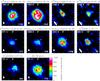 |
Fig. 3 Selected high-excitation line maps. The molecule, the frequency of the transition (in GHz), and the velocity range (in km s-1) are given above each panel. The color scale ranges from 0 to 1000 K km s-1 at 345/355 GHz, where the map size is 5′′, and from 0 to 100 K km s-1 at 690 GHz, where the map size is 10′′. Beams are shown in the lower left, and the number in the lower right of each panel is the maximum flux in K km s-1 (contours are ± 20 and 50% of that value). The energy of the lower level is given in the upper left. |
3.3. Line maps
From many maps of interesting lines (see Appendix, Fig. B.1), we show here only a selection, which is relevant to the expansion motion (Fig. 2) and the high excitation (Fig. 3). They are ordered as in Table 3. The velocity was integrated over the ranges with a detectable signal and no significant deviations in the channel maps, i.e., the whole flux for simple line shapes and several velocity ranges for more complex line shapes. For Fig. 2, we chose common velocity ranges for the four lines, which are 30 − 50 km s-1, representing the high-velocity part of the (front-side) outflow, 51 − 64 km s-1, the low-velocity part, 65 − 70 km s-1, the systemic velocity, and 71 − 84 km s-1, the low-velocity part of the back-side outflow. Higher velocities are not detected, probably due to dust absorption. In case of contamination by a neighboring line, the velocity range was chosen to avoid this line. Still, blending is likely for SO at 344.3 GHz by methanol (frequency corresponds to a 1.5 km s-1 lower velocity), H13CN at 345.3 GHz by SO2 (1 km s-1 higher velocity), H15NC at 355.4 GHz by CH3CH3CO (3.3 km s-1 lower velocity), and CH3NH2 at 354.8 GHz by CH3OCHO (3.8 km s-1 higher velocity).
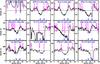 |
Fig. 4 Lines with absorption features toward the continuum peak. The systemic velocity of 68 km s-1 and a blue-shifted velocity of 50 km s-1 are marked. There are absorption components centered at both velocities, indicating expansion. The dashed horizontal line denotes the continuum level. |
3.4. Spectra
Figure 4 shows central spectra of the 12 transitions with absorption features. Most of the absorption is blue-shifted relative to the systemic velocity of 68 km s-1.
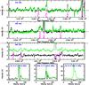 |
Fig. 5 Comparison of APEX data (green) to the SMA data convolved to the APEX beam (black). The dashed lines mark the continuum level as expected from LABOCA and SABOCA measurements. |
3.5. Comparison to APEX data
To estimate calibration and filtering of extended emission, we compared the SMA data to data from the APEX (Atacama Pathfinder Experiment) 12-m telescope (Güsten et al. 2006; Schuller et al. 2009; Rolffs et al. 2011b). The 345 GHz flux from the LABOCA bolometer array is 34 Jy/Beam, the 850 GHz flux from SABOCA is 450 Jy/Beam. At both frequencies, the source is unresolved with the beams of 18.2 and 7.4′′, respectively. The spectral index is 2.86, so the 690 GHz flux would be 250 Jy. The SMA fluxes at 210 and 345 GHz fit the APEX data very well, but at 690 GHz the continuum is much lower. This might be partly explained by decorrelation from fast phase fluctuations, and partly by missing short baselines that filter out extended emission.
Figure 5 shows APEX spectra overlaid with SMA spectra that were convolved to the APEX beam (18.2′′ at 345 GHz, 17.7′′ at 355 GHz, and 9.1′′ at 690 GHz). The lines match very well. Only the HCN and CO lines are affected by filtering of extended emission due to missing short spacings. The most notable example is CO 6–5, which is purely in absorption with the SMA, but has strong emission as seen with APEX (>1000 Jy). Extended emission of CO 6–5 is filtered out, leaving an apparent absorption towards the continuum, which is more compact, hence not affected as much as CO by the filtering.
4. Modeling
In this section, we compare a few models to continuum and vibrationally excited HCN in order to constrain the structure of this complex region, mainly density distribution and velocity field. Testing different models of the source structure allows exclusion of certain structures and an approach to the real structure by adapting the models. The models are inevitably simplified. We used a trial-and-error technique with parameter variations, and compared the model and data by eye to approach a good fit if possible for a tested structure, but no global optimization of fit parameters was performed.
The three-dimensional radiative-transfer code RADMC-3D8, developed by C. Dullemond, was employed to compute the dust temperature from stellar heating and the continuum and line emission of a model. The basic setup is the same as described in Rolffs et al. (2011a), but here we also test clumpiness and velocity structure in the models. The line transfer assumes LTE, which is a good approximation for vibrationally excited HCN, but prevents modeling of the ground-state lines. Molecular data are from Thorwirth et al. (2003) and Fuchs et al. (2004).
4.1. The models
While no perfect fit was found, we selected five of the tested models for presentation and comparison to the data. Models A and B have been previously used to fit APEX and VLA data of this source, respectively (Rolffs et al. 2011b,a). Model C has a radial density profile that best matches the observed continuum (if heated by the stars in the Hii regions). Models D and E have density fluctuations on small scales, which are expected from self-gravity and which improve the line fitting. Model E is an attempt to include the outflow (which is seen by the blue-shifted absorption features) and is presented in more detail.
The models are described explicitly in the following. Table 4 summarizes the main properties of the models.
Model A.
This is the model that was presented in Rolffs et al. (2011b) to fit the APEX data (continuum and many lines from HCN, HCO+, and CO, including vibrationally excited HCN). The density follows a radial power law,  H2 cm-3 for radii larger than 485 AU. Inside there is an Hii region with an electron density of 1.5 × 106 cm-3 to reproduce the free-free radiation from B1, and a star of 5.6 × 10⁵L⊙. The dust opacity is from Ossenkopf & Henning (1994) without grain mantles, but with coagulation at a density of 105 cm-3. The HCN abundance is 3 × 10⁻⁵ at temperatures above 100 K and 5 × 10⁻⁸ below 100 K. The line width is 5 km s-1 FWHM, and the gas is radially infalling with 1 km s-1 to the center at B1. The total mass (in a cube of 3 pc diameter) is 2.4 × 10⁴M⊙, of which 70 M⊙ are at temperatures above 300 K.
Model B.
This is the model that was presented in Rolffs et al. (2011a) to fit the VLA data of vibrationally excited HCN. The density follows a Gaussian, centered on B1, with 7 × 10⁷ H2 cm-3 at the half-maximum radius of 7000 AU. As in all subsequent models, heating sources are the stars in the Hii regions B1 with 105L⊙, B2 with 8.3 × 10⁴L⊙, and A with 4.6 × 10⁴L⊙, which are placed in the plane of the sky, and the dust opacity is from Ossenkopf & Henning (1994) without grain mantles or coagulation. The HCN abundance is 10-5. The intrinsic line width (FWHM) is 8.3 km s-1, and there is no macroscopic velocity field. The total mass is 3.5 × 10³M⊙, of which 350 M⊙ are at temperatures above 300 K.
Model C.
The density in this model follows a Plummer profile,  H2 cm-3 (half-maximum radius 6500 AU). It is centered 2000 AU south and 1000 AU west of B1. The Plummer model is very similar to a Gaussian inside the half-maximum radius, but has higher density outside (still falling off steeply as r-5). The HCN abundance is 10-5 at temperatures above 300 K and 10-6 below, as in the following models. The intrinsic line width (FWHM) is 8.3 km s-1, and there is no macroscopic velocity field. The total mass is 6.8 × 10³ M⊙, of which 350 M⊙ are at temperatures above 300 K.
Model D.
This model consists of 100 clumps, which have a Plummer half-maximum radius of 1000 AU and central densities ranging from 4 × 10⁸ to 2 × 10⁹ H2 cm-3. The distribution of clump masses follows the same slope as the stellar initial mass function. They are randomly placed in the model according to a Plummer distribution with a half-maximum radius 4000 AU. The density in each model cell is the maximum of all contributions from the clumps, so with a lot of overlap, this structure is more density fluctuation than separate cores. The intrinsic line width (FWHM) is 5 km s-1. Each clump has a random line-of-sight velocity with Gaussian half-maximum value of ± 5 km s-1. The line-of-sight velocity of each cell is an average of all clumps, weighted with their density contribution. The total mass is 9.4 × 10³M⊙, of which 470 M⊙ are at temperatures above 300 K.
Model E.
This model has the same structure as model D, but a half-maximum radius of the distribution of the clumps of only 3000 AU. In addition, a bipolar outflow is present, with an opening angle of 100° and a length of 2 × 10⁴ AU. Its center lies 1000 AU south and 500 AU west of B1. The axis is tilted from the line of sight by 20°, and the foreground part directed towards B2. Inside the outflow cone, the density is reduced to 20% of the original value (thus preserving the clumpy structure) and the velocity is 10 km s-1 outwards. This is only a toy model of the outflow. The total mass is 4.6 × 10³M⊙, of which 400 M⊙ are at temperatures above 300 K. The clumpy structure is visualized in Fig. 6.
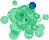 |
Fig. 6 Clumpy structure of model E displayed as isocontours of 107 H2 cm-3 (green, transparent). The Hii regions, whose stars heat up the gas, are shown in blue. The size of the contoured region is around 0.2 pc. |
4.2. Continuum
The continuum radiation that the models emit is compared to the data. Models D and E have randomly placed core centers; therefore their radiation (continuum and lines) have a random component, which cannot be reproduced exactly in different runs with the same parameters.
The radial profile of the 345/355 GHz continuum map is extracted with central position RA 18:08:38.237, Dec −19:51:50.421, which is the center of a two-dimensional Gaussian fit (1.4′′ × 1.17′′, elongated along the B1-B2 axis). The model maps were Fourier-transformed, folded with the uv-coverage of the observations, and imaged in the same way as the data. The radial profile of the model was extracted from the same central coordinates. Figure 7 shows a comparison of the radial profiles, and Fig. 8 a comparison of the continuum map of model E to the data. Model A (power-law) fits worse to the radial profile, model C (Plummer) fits best.
The flux from APEX/LABOCA (345 GHz) is 34 Jy/Beam (18.2′′ beam size) and from APEX/SABOCA (850 GHz) 450 Jy/Beam (7.4′′ beam size). The models emit 31 (A), 20 (B), 26 (C), 20 (D), and 18 (E) Jy/Beam for LABOCA and 266 (A), 231 (B), 311 (C), 146 (D), and 162 (E) Jy/Beam for SABOCA. In models B-E an extended component similar to A could be added without affecting the results of the interferometer modeling.
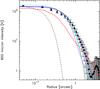 |
Fig. 7 Models A (red), B (green), C (blue), D (cyan), and E (magenta) compared to the SMA continuum profile, which is displayed as data points with a 0.1′′ radial interval. The errorbars denote the rms deviation from a circular shape, and the dashed curve represents the beam. |
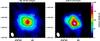 |
Fig. 8 Model E (right) compared to the SMA continuum map at 345 GHz (left). |
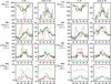 |
Fig. 9 Models A–D compared to lines from vibrationally excited HCN at the position of B1 and 0.3′′ (VLA) or 0.8′′ (SMA) south of B1. The left panel shows models A (red) and B (green), the right panel models C (red) and D (green). |
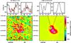 |
Fig. 10 Model E (right) compared to the J = 13 direct ℓ-type line of vibrationally excited HCN at 40.8 GHz (VLA), shown as an integrated line map and spectra at two locations (left, model spectra are overlaid in red). The white contours denote the 7 mm continuum in steps of 1000 K. |
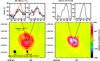 |
Fig. 11 Model E (right) compared to the J = 4 − 3 line of vibrationally excited HCN at 354.5 GHz (SMA), shown as integrated line map and spectra at two locations (left, model spectra are overlaid in red). The white contours denote the 355 GHz continuum in steps of 25 K. |
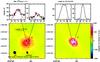 |
Fig. 12 Model E (right) compared to the J = 4 − 3 line of vibrationally excited H13CN at 345.2 GHz (SMA), shown as integrated line map and spectra at two locations (left, model spectra are overlaid in red). The white contours denote the 345 GHz continuum in steps of 25 K. |
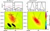 |
Fig. 13 Model E (right) compared to the J = 8 − 7 line of vibrationally excited H13CN at 690.4 GHz (SMA), shown as integrated line map and spectra at two locations (left, model spectra are overlaid in red). The white contours denote the 690 GHz continuum in steps of 25 K. |
4.3. Vibrationally excited HCN
The models are compared to lines from vibrationally excited HCN, including the J = 13 direct ℓ-type transition at 40.7669 GHz observed with the VLA (Rolffs et al. 2011a). Figure 9 shows this line and three rotational transitions of vibrationally excited HCN observed with the SMA, overlaid with models A–D. To reproduce the direct ℓ-type line, the rotational lines must be very optically thick, leading to self-absorption in the models. This is inevitable for optically thick lines from centrally heated spheres; the data however do not show self-absorption. The self-absorption decreases from model A to E. Model E is shown in detail in comparison to the J = 13 direct ℓ-type line of vibrationally excited HCN (Fig. 10), the 4–3 line of vibrationally excited HCN (Fig. 11) and H13CN (Fig. 12), and the 8–7 transition of vibrationally excited H13CN (Fig. 13). The outflow is imprinted in the line shapes. The levels of all these transitions lie between 1050 and 1400 K above ground.
5. Discussion
5.1. Chemistry
In addition to about 350 identified lines, there are around 90 unidentified (U-) lines, 75 of which are in the 201/211 GHz range, which covers a similar velocity range as the higher frequency bands combined (almost 6000 km s-1). This is probably due to the lower noise at these frequencies. The line density is mainly determined by the width of single lines (5–10 km s-1), i.e. a forest of overlapping lines covers most of the bands. The identified molecules (3 S-bearing, 10 N-bearing, and 9 other, O-bearing molecules) represent only the strongest lines, while more complex molecules have many weak lines that probably add up to the continuum and are undetectable owing to line confusion. No spatial separation of different molecules could be seen. The differences in the maps can probably be explained by excitation and optical depth.
In the detailed models (Sect. 4), the abundance of HCN in the hot gas is very high, on the order of 10-5 relative to H2. This is needed to reproduce the direct ℓ-type line and the vibrationally excited H13CN. Around 5% of the nitrogen and 1.4% of the carbon is in HCN (for solar N/H of 1.1 × 10⁻⁴ and C/H of 3.6 × 10⁻⁴, Anders & Grevesse 1989), and HCN/CO is on the order of 0.1 in the hot central region. We note that such a high HCN abundance needs an explanation by future chemical models, incorporating high-temperature reaction networks. The abundance of HC3N seems to follow a similar increase at high temperatures, as the strong emission from vibrational states suggests (Figs. A.1 − A.3). Notable line detections are HC15N, v2 = 1 at 691.6 GHz (lower level is 1139 K above ground), HC3N, v4 = v7 = 1 at 355.1 GHz (1908 K), and the 13C substituted HC3N, v7 = 2 (970 K). The H O line at 692.1 GHz (694 K) implies a high abundance of water in the dense, warm gas. These abundance enhancements could be connected, e.g., through a reduced abundance of OH, which at high temperatures reacts to form water instead of destroying N-bearing molecules (Rodgers & Charnley 2001).
5.2. Density distribution
As the high-resolution continuum map at 345/355 GHz shows, a power-law radial density is not consistent with the data. A Gaussian fits well in the inner part, but falls off too steeply in the outer parts. What fits best to the data is a Plummer model (Fig. 7). This profile is very similar to a Gaussian inside the half-maximum radius, but is denser outside, where it falls off as r-5. It is also used to describe the stellar density of star clusters. Although that might reveal a connection of this forming star cluster to later stages, it could also have completely different physical reasons. The stellar density distribution is determined by stellar dynamics, while the gas density distribution is determined by the interplay of different sources of pressure (gravitational versus turbulent, rotational, magnetic, radiative, and thermal pressure). The observed central flattening of the density can be explained by centrally increased pressure, which is expected from feedback by the newly formed massive stars. This pressure stalls the infall and piles up the mass where the infall stops, resulting in a less centrally peaked mass distribution.
The SMA continuum at 690 GHz is rather weak compared to the 345 GHz flux and the high-frequency single-dish flux. As interferometer observations at these frequencies are challenging, and only very few have been conducted yet (e.g. Beuther et al. 2006), this could come from the decorrelation caused by rapid phase noise. On the other hand, the line strengths are similar to the APEX data (Fig. 5), supporting the data quality and the calibration, so if the low continuum is real, it can result from optical depth effects in very dense, small condensations, while extended emission is filtered out. The continuum at 690 GHz must be more extended than at 345 GHz because the higher dust opacity makes it stronger only in the optically thin regions, while it can be weaker in the optically thick case; instead of the whole hot interior, one sees only up to the colder foreground. In addition, the image fidelity at 690 GHz is not as good as at 345 GHz; in particular, the shortest baselines are twice as large. As the flux rises with shorter baselines, this means much more filtering out of extended emission at 690 GHz.
Fragmentation is observed in neither the continuum nor the lines. The reason may be that we do not resolve structures smaller than the beam size of about 3000 AU. We note that the continuum source extends over about ten beams (3′′), so no large-scale fragmentation is present. Models of the line emission reveal that a spherical density distribution leads to strong self-absorption features, which are not observed. Clumpiness reproduces the line shapes better, but without sufficient spatial resolution we cannot derive the properties of fragmentation.
This missing fragmentation is similar to the contiuum data recently obtained by Qin et al. (2011) for SgrB2-N, which follows a very similar radial profile and also displays a similar spectral line content. Maybe the two sources are at the same evolutionary stage, where the first hypercompact Hii regions have developed and heated the gas, but large-scale fragmentation has not set in.
The rotational transition of vibrationally excited HCN (4 − 3 at 354.46 GHz) has a very high optical depth. The Einstein A coefficient is 50 000 times higher than for the direct ℓ-type line (J = 13 at 40.7669 GHz, observed with the VLA), which has an optical depth of ≲ 1. Also the comparison to the H13CN line (Fig. 3) shows its high optical depth. In models that are homogeneous on small scales (smooth density gradient, such as models A–C), this optically thick line is self-absorbed owing to the temperature gradients caused by internal heating. Such large temperature gradients are inevitable as the stars must be deeply embedded, shown by the high efficiency of heating and the compactness of the Hii regions. The observed single-peaked profile can only be explained by an inhomogeneous density and velocity field (such as models D–E), where the self-absorption is smeared out. Such small-scale clumpiness might persist in later stages of evolution, when the gas is ionized (Ignace & Churchwell 2004).
The observed continuum depends on density, temperature, and dust opacity. The density can vary by many orders of magnitude, and therefore dominates the resulting continuum. It is clear that the temperature is high in the inner region and falls off outwards, and this is included in the models as the stars in the hypercompact Hii regions heat the dust. It is entirely possible, however, that more heating sources are present, although they are not needed for heating the central region. The extension of high-excitation lines is generally a bit smaller in the models than in the data, especially highly excited HC3N is somewhat extended to the east (Fig. 3).
5.3. Velocity field
While most lines do not show any velocity structure in their maps, there seems to be a component of highly excited CH3OH at lower velocity close to the UCHii region A (Fig. 3). Alternatively, this could arise from blending by a different line.
On large scales, the asymmetries of self-absorbed lines clearly indicate infall motions (Rolffs et al. 2011b, and Fig. 5), and also the absorption of the H2CO line is a bit red-shifted (Fig. 4). On smaller scales, we see expansion motions, as very nicely traced by the absorption features (Fig. 4). The blue-shifted absorption is stronger in the western part of the continuum. In addition, the SO line at 344.3 GHz, the HCN line at 354.5 GHz, and the CO line at 345.8 GHz have red-shifted emission in the northeastern part. A red-shifted clump 5′′ north of the hot core, which is only seen in HCN and CO, seems to be too far away to be related to the outflow (Fig. 2).
Olmi et al. (1996) detected a north-south velocity gradient in 13CO, and Hofner & Churchwell (1996) see blue-shifted water masers 0.2′′ north and 0.4′′ south of B1, and a red-shifted water maser (at 70 km s-1) 1.2′′ north of B1. Absorption against the hypercompact Hii regions B1 and B2 is found to be blue-shifted in NH3(4, 4) (Cesaroni et al. 2010, 53 km s-1 toward B1 and 61 km s-1 toward B2), and also partly in vibrationally excited HCN (Rolffs et al. 2011a, and Fig. 10).
One can conclude that there is likely to be a bipolar outflow, whose foreground part is tilted to the southwest, and whose background part is tilted to the northeast. A sketch of the outflow scenario is presented in Fig. 14. This scenario explains all observed velocity features qualitatively. The different NH3(4, 4) velocities, for instance, can be understood as an effect of the projection of the outflow to the line-of-sight. An embedded source, which has not yet developed a detectable Hii region, is driving the outflow in this scenario. A nearly spherical infall with lower velocity, but higher rate than the expansion surrounds the outflow and produces the blue asymmetric line profiles seen on larger scales. This accretion probably continues well into the central region along certain paths, driven by gravitational attraction and the momentum of the large-scale accretion flow.
An alternative scenario might arise if the hypercompact Hii regions B1 and B2 are not spherical, but in the form of bipolar expanding bubbles from a photoevaporating disk (Hollenbach et al. 1994). In this case, the stars in the HCHii regions would drive two outflows, which are both roughly aligned with the line-of-sight.
In addition, it is possibile that the source is a large pseudo-disk accreting from a massive envelope, rotating roughly in the plane of the sky, driving an outflow perpendicular to it, and having formed B1 and B2 as binaries (and maybe more stars). This would correspond to the transition between phases II and III of Zapata et al. (2010).
A quantitative radiative transfer model, which reproduces all observed lines, is possible, but beyond the scope of this paper. That the outflow is important for reproducing the line shapes has been demonstrated in our modeling, as only model E could reproduce the shapes (Sect. 4).
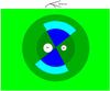 |
Fig. 14 Qualitative scenario for the outflow in G10.47+0.03. The observer is above the plot. Infalling molecular gas is shown in green, expanding molecular gas in blue, and ionized gas in white. The circles denote half-maximum and Plummer radius in Model C (the gas must be clumpy, though) and the boundaries of the Hii regions, which have density gradients (Cesaroni et al. 2010). If the Hii regions are not spherical, the outflow could also develop from the ionizing stars. |
6. Conclusions
With the SMA, we have obtained high-resolution, spectrally resolved maps of the massive hot molecular core G10.47+0.03 at different frequencies, covering a bandwidth of 12 GHz in total and including observations at 690 GHz. Our main results follow.
-
Hundreds of molecular lines reveal a rich chemistry, with molecules such as HCN and HC3N especially abundant at high temperatures. This high abundance demands explanations from chemical models. Vibrationally excited HCN, whose levels lie more than 1000 K above ground, is very optically thick, and even vibrationally excited HC15N shows up at 690 GHz.
-
Blue-shifted absorption in a dozen lines indicates an outflow oriented roughly along the line-of-sight. It is embedded as there is also absorption at the systemic velocity of cold foreground gas in CO and HCN.
-
The averaged radial profile of the submm continuum displays a central flattening and rapid falloff, and is best fitted by a Plummer profile of the density. The mass of the source is on the order of several thousand M⊙, of which a few hundred are at high ( > 300 K) temperatures.
-
No fragmentation is observed over the ~10 beam sizes (30 000 AU) of the continuum emission. High-excitation lines that are very optically thick do not show self-absorption. The line modeling suggests that this must be due to density fluctuations in combination with the velocity field. If the rather low continuum at 690 GHz is real, it points to small, very dense condensations.
From these findings, a picture emerges of a very young forming star cluster, characterized by the beginning of feedback from massive stars, while infall is ongoing. This feedback includes heating of the dust and gas, ionization that is still confined to small regions, and increased pressure in the inner part that leads to expansion motions and central flattening of the density.
Online material
Appendix A: Full spectral range
In Figs. A.1−A.3, we show the full observed spectral range, convolved to a resolution of 5′′, and label the identified lines with the molecule (see also Sect. 3.2).
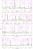 |
Fig. A.1 Full spectral range towards G10.47+0.03 convolved to 5′′ resolution. The green overlay is the myXLASS model for all molecules except HC3N, whose emission is overlaid in red. The displayed panels cover 199.85–201.85 GHz (upper three) and 209.85–210.55 GHz (bottom); the rest is shown in Figs. A.2 and A.3. |
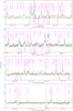 |
Fig. A.3 As in Fig. A.1, displaying 354.1–355.95 GHz (upper two), 680.2–682.3 GHz (third panel from top), and 690.2–692.3 GHz (bottom). |
Appendix B: Line maps
In Fig. B.1 we show 100 integrated line maps, ordered by molecule as in Table 3 and by frequency of the transition (see also Sect. 3.3).
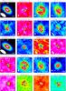 |
Fig. B.1 Integrated line maps. Above each panel, the molecule, the frequency of the transition (in GHz), and the velocity range (in km s-1) are given. The map size is either 5, 10, or 15′′, as written in the map (tick spaces are 1′′, centered on RA 18:08:38.236, Dec –19:51:50.25). Beams are shown in the lower left, and the number in the lower right of each panel is the maximum flux in K km s-1 (the contours are ± 20 and 50% of that value). The color scale ranges from the minimum to the maximum value. The energy of the lower level is given in the upper left. |
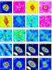 |
Fig. B.1 continued. |
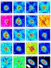 |
Fig. B.1 continued. |
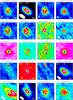 |
Fig. B.1 continued. |
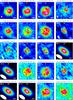 |
Fig. B.1 continued. |
The Submillimeter Array is a joint project between the Smithsonian Astrophysical Observatory and the Academia Sinica Institute of Astronomy and Astrophysics and is funded by the Smithsonian Institution and the Academia Sinica (Ho et al. 2004).
Acknowledgments
We are grateful to Mark Gurwell for his help with reducing the 690 GHz data, and to Kees Dullemond for kindly providing us with the RADMC-3D code. R. Rolffs acknowledges support from the International Max Planck Research School (IMPRS) for Astronomy and Astrophysics.
References
- Anders, E., & Grevesse, N. 1989, Geochim. Cosmochim. Acta, 53, 197 [Google Scholar]
- Beuther, H., Zhang, Q., Reid, M. J., et al. 2006, ApJ, 636, 323 [NASA ADS] [CrossRef] [Google Scholar]
- Cesaroni, R. 2005, in Massive Star Birth: A Crossroads of Astrophysics, ed. R. Cesaroni, M. Felli, E. Churchwell, & M. Walmsley, IAU Symp., 227, 59 [Google Scholar]
- Cesaroni, R., Hofner, P., Araya, E., & Kurtz, S. 2010, A&A, 509, A50 [NASA ADS] [CrossRef] [EDP Sciences] [Google Scholar]
- Fuchs, U., Bruenken, S., Fuchs, G. W., et al. 2004, Z. Naturforsch. A, 59, 861 [NASA ADS] [Google Scholar]
- Güsten, R., Nyman, L. Å., Schilke, P., et al. 2006, A&A, 454, L13 [NASA ADS] [CrossRef] [EDP Sciences] [Google Scholar]
- Ho, P. T. P., Moran, J. M., & Lo, K. Y. 2004, ApJ, 616, L1 [NASA ADS] [CrossRef] [Google Scholar]
- Hoare, M. G., Kurtz, S. E., Lizano, S., Keto, E., & Hofner, P. 2007, Protostars and Planets V, 181 [Google Scholar]
- Hofner, P., & Churchwell, E. 1996, A&AS, 120, 283 [NASA ADS] [CrossRef] [EDP Sciences] [Google Scholar]
- Hollenbach, D., Johnstone, D., Lizano, S., & Shu, F. 1994, ApJ, 428, 654 [NASA ADS] [CrossRef] [Google Scholar]
- Ignace, R., & Churchwell, E. 2004, ApJ, 610, 351 [NASA ADS] [CrossRef] [Google Scholar]
- Kurtz, S., Cesaroni, R., Churchwell, E., Hofner, P., & Walmsley, C. M. 2000, Protostars and Planets IV, 299 [Google Scholar]
- Müller, H. S. P., Schlöder, F., Stutzki, J., & Winnewisser, G. 2005, J. Mol. Struct., 742, 215 [NASA ADS] [CrossRef] [Google Scholar]
- Müller, H. S. P., Thorwirth, S., Roth, D. A., & Winnewisser, G. 2001, A&A, 370, L49 [NASA ADS] [CrossRef] [EDP Sciences] [Google Scholar]
- Olmi, L., Cesaroni, R., Neri, R., & Walmsley, C. M. 1996, A&A, 315, 565 [NASA ADS] [Google Scholar]
- Ossenkopf, V., & Henning, T. 1994, A&A, 291, 943 [NASA ADS] [Google Scholar]
- Pandian, J. D., Momjian, E., & Goldsmith, P. F. 2008, A&A, 486, 191 [NASA ADS] [CrossRef] [EDP Sciences] [Google Scholar]
- Pickett, H. M., Poynter, R. L., Cohen, E. A., et al. 1998, J. Quant. Spec. Radiat. Transf., 60, 883 [Google Scholar]
- Qin, S.-L., Schilke, P., Rolffs, R., et al. 2011, A&A, 530, L9 [NASA ADS] [CrossRef] [EDP Sciences] [Google Scholar]
- Rodgers, S. D., & Charnley, S. B. 2001, ApJ, 546, 324 [Google Scholar]
- Rolffs, R., Schilke, P., Wyrowski, F., et al. 2011a, A&A, 529, A76 [NASA ADS] [CrossRef] [EDP Sciences] [Google Scholar]
- Rolffs, R., Schilke, P., Wyrowski, F., et al. 2011b, A&A, 527, A68 [NASA ADS] [CrossRef] [EDP Sciences] [Google Scholar]
- Sault, R. J., Teuben, P. J., & Wright, M. C. H. 1995, in Astronomical Data Analysis Software and Systems IV, ed. R. A. Shaw, H. E. Payne, & J. J. E. Hayes, ASP Conf. Ser., 77, 433 [Google Scholar]
- Schuller, F., Menten, K. M., Contreras, Y., et al. 2009, A&A, 504, 415 [NASA ADS] [CrossRef] [EDP Sciences] [Google Scholar]
- Thorwirth, S., Müller, H. S. P., Lewen, F., et al. 2003, ApJ, 585, L163 [NASA ADS] [CrossRef] [Google Scholar]
- Wyrowski, F., Schilke, P., & Walmsley, C. M. 1999, A&A, 341, 882 [NASA ADS] [Google Scholar]
- Zapata, L. A., Tang, Y., & Leurini, S. 2010, ApJ, 725, 1091 [NASA ADS] [CrossRef] [Google Scholar]
- Zinnecker, H., & Yorke, H. W. 2007, ARA&A, 45, 481 [NASA ADS] [CrossRef] [Google Scholar]
All Tables
All Figures
|
Fig. 1 Continuum maps of G10.47+0.03 observed with the SMA at 201/211 GHz (top panel), 345/355 GHz (central), and 681/691 GHz (bottom). The map size is either 5 or 10′′. Contours mark 20 and 50% of the peak flux, which is given in the lower right (in K). The beam is depicted in the lower left. The white crosses denote the Hii regions B1, B2, and A (Cesaroni et al. 2010, from left to right). |
| In the text | |
|
Fig. 2 Line maps (selected to trace expansion motions) integrated over the velocity range indicated in each panel (which can be considered, from left to right, as the high-velocity part of the outflow, low-velocity part, systemic velocity, and low-velocity part of the outflow at the far side). The first velocity range of HC3N is blended by other lines. In the second velocity range of CO the emission is extended this much to cause imaging artifacts. The map size is 5′′ (tick spaces are 1′′, centered on RA 18:08:38.236, Dec –19:51:50.25). Beams are shown in the lower left, and the number in the lower right of each panel is the maximum flux in K km s-1 (contours are ± 20 and 50% of that value). The color scale is from –1000 to 1000 K km s-1. The energy of the lower level is given in the upper left. |
| In the text | |
|
Fig. 3 Selected high-excitation line maps. The molecule, the frequency of the transition (in GHz), and the velocity range (in km s-1) are given above each panel. The color scale ranges from 0 to 1000 K km s-1 at 345/355 GHz, where the map size is 5′′, and from 0 to 100 K km s-1 at 690 GHz, where the map size is 10′′. Beams are shown in the lower left, and the number in the lower right of each panel is the maximum flux in K km s-1 (contours are ± 20 and 50% of that value). The energy of the lower level is given in the upper left. |
| In the text | |
|
Fig. 4 Lines with absorption features toward the continuum peak. The systemic velocity of 68 km s-1 and a blue-shifted velocity of 50 km s-1 are marked. There are absorption components centered at both velocities, indicating expansion. The dashed horizontal line denotes the continuum level. |
| In the text | |
|
Fig. 5 Comparison of APEX data (green) to the SMA data convolved to the APEX beam (black). The dashed lines mark the continuum level as expected from LABOCA and SABOCA measurements. |
| In the text | |
|
Fig. 6 Clumpy structure of model E displayed as isocontours of 107 H2 cm-3 (green, transparent). The Hii regions, whose stars heat up the gas, are shown in blue. The size of the contoured region is around 0.2 pc. |
| In the text | |
|
Fig. 7 Models A (red), B (green), C (blue), D (cyan), and E (magenta) compared to the SMA continuum profile, which is displayed as data points with a 0.1′′ radial interval. The errorbars denote the rms deviation from a circular shape, and the dashed curve represents the beam. |
| In the text | |
|
Fig. 8 Model E (right) compared to the SMA continuum map at 345 GHz (left). |
| In the text | |
|
Fig. 9 Models A–D compared to lines from vibrationally excited HCN at the position of B1 and 0.3′′ (VLA) or 0.8′′ (SMA) south of B1. The left panel shows models A (red) and B (green), the right panel models C (red) and D (green). |
| In the text | |
|
Fig. 10 Model E (right) compared to the J = 13 direct ℓ-type line of vibrationally excited HCN at 40.8 GHz (VLA), shown as an integrated line map and spectra at two locations (left, model spectra are overlaid in red). The white contours denote the 7 mm continuum in steps of 1000 K. |
| In the text | |
|
Fig. 11 Model E (right) compared to the J = 4 − 3 line of vibrationally excited HCN at 354.5 GHz (SMA), shown as integrated line map and spectra at two locations (left, model spectra are overlaid in red). The white contours denote the 355 GHz continuum in steps of 25 K. |
| In the text | |
|
Fig. 12 Model E (right) compared to the J = 4 − 3 line of vibrationally excited H13CN at 345.2 GHz (SMA), shown as integrated line map and spectra at two locations (left, model spectra are overlaid in red). The white contours denote the 345 GHz continuum in steps of 25 K. |
| In the text | |
|
Fig. 13 Model E (right) compared to the J = 8 − 7 line of vibrationally excited H13CN at 690.4 GHz (SMA), shown as integrated line map and spectra at two locations (left, model spectra are overlaid in red). The white contours denote the 690 GHz continuum in steps of 25 K. |
| In the text | |
|
Fig. 14 Qualitative scenario for the outflow in G10.47+0.03. The observer is above the plot. Infalling molecular gas is shown in green, expanding molecular gas in blue, and ionized gas in white. The circles denote half-maximum and Plummer radius in Model C (the gas must be clumpy, though) and the boundaries of the Hii regions, which have density gradients (Cesaroni et al. 2010). If the Hii regions are not spherical, the outflow could also develop from the ionizing stars. |
| In the text | |
|
Fig. A.1 Full spectral range towards G10.47+0.03 convolved to 5′′ resolution. The green overlay is the myXLASS model for all molecules except HC3N, whose emission is overlaid in red. The displayed panels cover 199.85–201.85 GHz (upper three) and 209.85–210.55 GHz (bottom); the rest is shown in Figs. A.2 and A.3. |
| In the text | |
 |
Fig. A.2 As in Fig. A.1, displaying 210.5–211.85 GHz (upper two) and 344.05–345.95 GHz (lower two). |
| In the text | |
|
Fig. A.3 As in Fig. A.1, displaying 354.1–355.95 GHz (upper two), 680.2–682.3 GHz (third panel from top), and 690.2–692.3 GHz (bottom). |
| In the text | |
|
Fig. B.1 Integrated line maps. Above each panel, the molecule, the frequency of the transition (in GHz), and the velocity range (in km s-1) are given. The map size is either 5, 10, or 15′′, as written in the map (tick spaces are 1′′, centered on RA 18:08:38.236, Dec –19:51:50.25). Beams are shown in the lower left, and the number in the lower right of each panel is the maximum flux in K km s-1 (the contours are ± 20 and 50% of that value). The color scale ranges from the minimum to the maximum value. The energy of the lower level is given in the upper left. |
| In the text | |
|
Fig. B.1 continued. |
| In the text | |
|
Fig. B.1 continued. |
| In the text | |
|
Fig. B.1 continued. |
| In the text | |
|
Fig. B.1 continued. |
| In the text | |
Current usage metrics show cumulative count of Article Views (full-text article views including HTML views, PDF and ePub downloads, according to the available data) and Abstracts Views on Vision4Press platform.
Data correspond to usage on the plateform after 2015. The current usage metrics is available 48-96 hours after online publication and is updated daily on week days.
Initial download of the metrics may take a while.