| Issue |
A&A
Volume 535, November 2011
|
|
|---|---|---|
| Article Number | A48 | |
| Number of page(s) | 12 | |
| Section | Astrophysical processes | |
| DOI | https://doi.org/10.1051/0004-6361/201116705 | |
| Published online | 03 November 2011 | |
The fratricide of αΩ dynamos by their α2 siblings
1
Nordita, AlbaNova University Center,
Roslagstullsbacken 23,
10691
Stockholm,
Sweden
e-mail: This email address is being protected from spambots. You need JavaScript enabled to view it.
2
Department of Astronomy, Stockholm University,
10691
Stockholm,
Sweden
Received:
13
February
2011
Accepted:
2
September
2011
Abstract
Context. Helically forced magneto-hydrodynamic shearing-sheet turbulence can support different large-scale dynamo modes, although the αΩ mode is generally expected to dominate because it is the fastest growing one. In an αΩ dynamo, most of the field amplification is produced by the shear. As differential rotation is an ubiquitous source of shear in astrophysics, such dynamos are believed to be the source of most astrophysical large-scale magnetic fields.
Aims. We study the stability of oscillatory migratory αΩ type dynamos in turbulence simulations.
Methods. We use shearing-sheet simulations of hydromagnetic turbulence that is helically forced at a wavenumber that is about three times larger than the lowest wavenumber in the domain so that both αΩ and α2 dynamo action is possible.
Results. After initial dominance and saturation, the αΩ mode is found to be destroyed by an orthogonal α2 mode sustained by the helical turbulence alone. We show that there are at least two processes through which this transition can occur.
Conclusions. The fratricide of αΩ dynamos by its α2 sibling is discussed in the context of grand minima of stellar activity. However, the genesis of αΩ dynamos from an α2 dynamo has not yet been found.
Key words: Sun: dynamo / magnetohydrodynamics (MHD) / dynamo
© ESO, 2011
1. Introduction
The observed existence of large-scale astrophysical magnetic fields, for example galactic or solar fields, is usually explained by self-excited dynamo action within electrically conducting fluids or plasmas. However, this mechanism of field amplification continues to be a matter of debate as the existing theory encounters problems when extrapolated to the large magnetic Reynolds numbers of astrophysics. Nonetheless, large-scale astrophysical fields are believed to be predominately generated by so-called αΩ dynamos, in which most of the field amplification occurs through the shearing of field lines by ubiquitous differential rotation, a process known as the Ω effect (Steenbeck & Krause 1969). For example, many models of the solar dynamo invoke the strong shear found in the tachocline at the base of the convection zone (see, e.g., Charbonneau 2010). Shear alone cannot drive dynamo action however, and the α effect, caused by helical motions, provides the necessary twist of the sheared field to complete the magnetic field amplification cycle. In the Sun, an α effect is provided via kinetic helicity due to the interaction of stratified convection and solar rotation.
The α effect can drive a dynamo by itself, which is then of the so-called α2 type. These dynamos are of great theoretical interest due to their simplicity, but are expected to be outperformed by αΩ dynamos in the wild. Strictly speaking, αΩ dynamos should be referred to as α2Ω dynamos as the α2 process of course continues to occur in reality, even in the presence of the Ω effect. However, in the mean-field approach one sometimes makes the so-called “αΩ” approximation by neglecting the production of toroidal field via the α effect entirely in favor of the Ω effect. In such models, the nonlinear competition between different αΩ modes has been thoroughly studied by monitoring, for example, rapid changes of Lyapunov exponents in the bifurcation structure (Covas et al. 1997).
In the present paper we consider numerical solutions of the compressible MHD equations in three dimensions with turbulent helical flows where, of course, the αΩ approximation is not applicable. Nevertheless we will refer to αΩ and α2Ω regimes when shear is dominant or comparable with amplification by the helical turbulence, respectively.
Very often, a linear stability analysis of a given setup reveals that several different dynamo modes are expected to be excited at the same time. While during the linear stage the relative strength of these modes is determined by the initial conditions, the mode or mixture of modes of the final saturated state is decided by the nonlinear interactions between the modes in their backreaction on the flow. The naive guess that the final state should always be characterized by the mode with the highest growth rate, has turned out not to be valid in general. This was first shown in Brandenburg et al. (1989), who found that, for small enough dynamo numbers, the saturated state of α2 and αΩ dynamos is instead determined by the solution with the smallest marginal dynamo number. For larger dynamo numbers, however, axisymmetric dipolar and quadrupolar modes have asymptotically identical growth rates, and in the nonlinear regime there can be several stable solutions, including some with mixed parity, that no longer bifurcate from the trivial one. Moreover, certain axisymmetric solutions turned out to be unstable to non-axisymmetric perturbations and evolved eventually toward another axisymmetric solution (Rädler et al. 1990).
In direct numerical simulations of a geodynamo model with stress-free boundary conditions, it has been observed that again two different dynamo solutions, a dipolar and a “hemispherical” one, can both be stable (Christensen et al. 1999; Grote & Busse 2000). Because of the free fluid surface in that model, this might even be taken as a hint for the possibility of non-unique stable states in stellar setups as well.
Fuchs et al. (1999) have demonstrated an even more extreme case with a dynamo powered by a forced laminar flow. In the course of the magnetic field growth, the Lorentz force arranges the flow into a different pattern, which is hydrodynamically stable, but unable to drive a dynamo. As the dynamo dies out subsequently without a chance to recover, it was named “suicidal”.
Hence, the question of the character of the final, saturated stage of a dynamo cannot reliably be answered on the basis of a linear approach and the study of the nonlinear model might unveil very unexpected results. Here, we will show in a simple setup that, while αΩ dynamos do grow faster than α2 dynamos, non-linear effects are capable of driving transitions from αΩ modes to α2 modes. As the two competing dynamo modes are excited for the same parameter set, i.e., are solutions of the same eigenvalue problem, we refer to them as fratricidal, in reminiscence of the aforementioned suicidal dynamos.
The two astrophysical dynamos for which we have long time-series, the solar dynamo and that of the Earth, both exhibit large fluctuations. The solar dynamo in particular is known to go through prolonged quiescent phases such as the Maunder minimum (Eddy 1976). A conceivable connection with fratricidal dynamos makes understanding how non-linear effects define large-scale dynamo magnetic field strengths and geometries a matter of more than intellectual curiosity.
In Sect. 2 we sketch the mean-field theory of α2 and α2Ω dynamos. In Sect. 3 we describe our numerical set-up and briefly discuss the test-field method, a technique to extract the turbulent transport coefficients of mean-field theory from direct numerical simulations. In Sects. 5 and 6 we describe different transition types, and we conclude in Sect. 7.
2. Mean field modeling
In the magneto-hydrodynamic approximation, the evolution of magnetic fields is controlled
by the induction equation 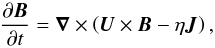 (1)where
B is the magnetic field,
J = ∇ × B
is the current density in units where the vacuum permeability is unity, and
η is the microphysical resistivity. A common approach to (1)is mean-field theory, under which physical
quantities (upper case) are decomposed into mean (overbars) and fluctuating (lower case)
constituents:
(1)where
B is the magnetic field,
J = ∇ × B
is the current density in units where the vacuum permeability is unity, and
η is the microphysical resistivity. A common approach to (1)is mean-field theory, under which physical
quantities (upper case) are decomposed into mean (overbars) and fluctuating (lower case)
constituents:  (2)The mean can be any which
obeys the Reynolds averaging rules, but is frequently assumed to be a spatial one filtering
out large length-scales (a two-scale approach). Here we will however use planar averaging,
either over the xy plane so that
(2)The mean can be any which
obeys the Reynolds averaging rules, but is frequently assumed to be a spatial one filtering
out large length-scales (a two-scale approach). Here we will however use planar averaging,
either over the xy plane so that
 or over
the yz plane, that is,
or over
the yz plane, that is,
 , where
⟨ · ⟩ ξ denotes averaging over all values of the variable
ξ (or volume, if not specified). A mean defined by averaging over
y only will also be used (⟨ · ⟩ y). We
humbly ask the reader to consider these definitions carefully, given that the two planar
averages will in places be used simultaneously. It is important to remember that the
superscript refers to the direction of variation, rather than the direction of averaging.
, where
⟨ · ⟩ ξ denotes averaging over all values of the variable
ξ (or volume, if not specified). A mean defined by averaging over
y only will also be used (⟨ · ⟩ y). We
humbly ask the reader to consider these definitions carefully, given that the two planar
averages will in places be used simultaneously. It is important to remember that the
superscript refers to the direction of variation, rather than the direction of averaging.
Under Reynolds averaging Eq. (1)becomes
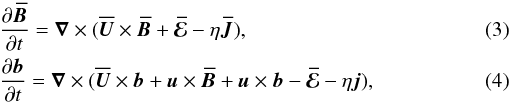 where
where
 is the
mean electromotive force (EMF) associated with correlations of the fluctuating fields.
is the
mean electromotive force (EMF) associated with correlations of the fluctuating fields.
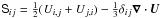
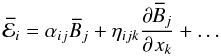
Symmetry considerations allow one to write the  as a
function of the mean-fields in the system. In the case of a planar averaging scheme, this
relation becomes
as a
function of the mean-fields in the system. In the case of a planar averaging scheme, this
relation becomes 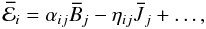 (5)where
αij and
ηij are turbulent transport coefficients,
and averaged quantities depend on one spatial coordinate only. The traditional
α effect is described by the symmetric part of the tensor
αij, and requires helicity in the flow. The
symmetric part of ηij describes turbulent
dissipation, and, in the isotropic case, appears equivalently to the microphysical
resistivity η. It is therefore termed the turbulent
resistivity, ηt. When assuming that
can be
completely represented by the mean magnetic field and its first spatial derivatives, the
Taylor series in (5)can be truncated after
the term
(5)where
αij and
ηij are turbulent transport coefficients,
and averaged quantities depend on one spatial coordinate only. The traditional
α effect is described by the symmetric part of the tensor
αij, and requires helicity in the flow. The
symmetric part of ηij describes turbulent
dissipation, and, in the isotropic case, appears equivalently to the microphysical
resistivity η. It is therefore termed the turbulent
resistivity, ηt. When assuming that
can be
completely represented by the mean magnetic field and its first spatial derivatives, the
Taylor series in (5)can be truncated after
the term  . A more complete formula
would include higher spatial as well as temporal derivatives.
. A more complete formula
would include higher spatial as well as temporal derivatives.
2.1. Mean-field dynamo action
Let us assume a large-scale shearing flow of the simple form  (6)and velocity fluctuations
which are isotropic, homogeneous, and statistically stationary. Consequently, if
αij and
ηij are assumed to be independent of
(6)and velocity fluctuations
which are isotropic, homogeneous, and statistically stationary. Consequently, if
αij and
ηij are assumed to be independent of
 (the
kinematic limit), then they reduce to constant scalars α and
ηt1.
(the
kinematic limit), then they reduce to constant scalars α and
ηt1.
If this system were to contain a y-dependent mean field, the shear would
induce field constituents which are proportional to x. We restrict
ourselves here to periodic spatial dependencies and hence exclude such unbounded fields.
When identifying the y direction with the azimuthal one in a spherical
system, this is equivalent to restricting to axisymmetric fields. The evolution of
harmonic mean magnetic fields is given by the solution of the eigenvalue problem
![Mathematical equation: \begin{equation} \label{MFE} \lambda\ithat\BB= \left[\begin{array}{ccc} -\etaT k^2 & -{\rm i}\alpha k_z & 0 \\ {\rm i}\alpha k_z+S & -\etaT k^2 & -{\rm i}\alpha k_x \\ 0 & {\rm i}\alpha k_x & -\etaT k^2 \end{array}\right] \ithat\BB, \end{equation}](/articles/aa/full_html/2011/11/aa16705-11/aa16705-11-eq32.png) (7)where
(7)where
 ,
ηT = ηt + η,
and
,
ηT = ηt + η,
and  . The
resulting dispersion relation reads
. The
resulting dispersion relation reads ![Mathematical equation: \begin{equation} (\lambda+\etaT k^2)[(\lambda+\etaT k^2)^2-\alpha^2k^2+\ii \alpha S k_z]=0, \label{disp} \end{equation}](/articles/aa/full_html/2011/11/aa16705-11/aa16705-11-eq36.png) (8)with eigenvalues (apart
from the always decaying modes with By = 0)
(8)with eigenvalues (apart
from the always decaying modes with By = 0)
 (9)It can easily be seen
that there are two “pure” modes with particularly simple geometries: the
α2 mode with
kz = 0 does not depend on S
and has the form
(9)It can easily be seen
that there are two “pure” modes with particularly simple geometries: the
α2 mode with
kz = 0 does not depend on S
and has the form
![Mathematical equation: \begin{equation} \BBa=\Bha \left[ 0,\, \sin k_x x,\, \pm\cos k_x x \right], \label{Balp} \end{equation}](/articles/aa/full_html/2011/11/aa16705-11/aa16705-11-eq41.png) (10)where the growth
rate is
(10)where the growth
rate is  and
and
 is an amplitude factor. The upper (lower) sign corresponds to positive (negative)
αkx.
is an amplitude factor. The upper (lower) sign corresponds to positive (negative)
αkx.
In contrast, the α2Ω mode with
kx = 0 does depend on S
and has, for
S ≫ αkz
(the αΩ approximation) the form
![Mathematical equation: \begin{eqnarray} \BBao&=&\Bhao \left[ \sin\! \big(k_z(z-ct)\big), \sqrt{2} \left| \frac{c}{\alpha}\right| \sin\! \big( k_z (z-ct) + \phi\big),0\right]\!,\label{BaO}\\ c&=& \operatorname{sign}(\alpha S)\sqrt{|\alpha S/2k_z|}. \label{CaO} \end{eqnarray}](/articles/aa/full_html/2011/11/aa16705-11/aa16705-11-eq47.png) In
the above,
In
the above,
 is again an amplitude factor, φ represents, for
S > 0
(S < 0), the
± π/4 (± 3π/4)
phase shift between the x and y components of the mean
field, and upper (lower) signs apply for positive (negative) values of
αkz; see Table 3 of Brandenburg & Subramanian (2005). The
corresponding growth rate is
is again an amplitude factor, φ represents, for
S > 0
(S < 0), the
± π/4 (± 3π/4)
phase shift between the x and y components of the mean
field, and upper (lower) signs apply for positive (negative) values of
αkz; see Table 3 of Brandenburg & Subramanian (2005). The
corresponding growth rate is  (13)For equal
|k|, the αΩ mode grows faster than
the α2 mode2.
(13)For equal
|k|, the αΩ mode grows faster than
the α2 mode2.
A key characteristic of α2Ω solutions is that the growth rate λ has a non-vanishing imaginary part kzc which results in traveling waves with phase speed c. The wave nature of α2Ω solutions is a significant draw in explaining the solar magnetic cycle. For a characteristic α2Ω dynamo found in direct numerical simulations with a setup described below, we show in Fig. 1 the time-series of rms values of B alongside the traveling wave in the z − t plane (“butterfly diagram”). This solution is similar to those considered recently by Käpylä & Brandenburg (2009). There are other sources for such oscillations however. Admittance of a spatially varying α enables oscillatory and hence traveling wave solutions in pure α2 dynamos, see Baryshnikova & Shukurov (1987), Rädler & Bräuer (1987), Stefani & Gerbeth (2003), Mitra et al. (2010).
The mean fields of α2 modes are force free, while α2Ω modes cause a potential force which has minimal effect as long as the peak Alfvén speed is subsonic so that the magnetic force cannot generate significant density perturbations. Within kinematics, the induction equation allows for superimposed α2 and α2Ω modes. Such a superposition can extend approximately into the non-kinematic regime, and in Sect. 5 we will discuss the implications of the Lorentz forces generated when this occurs.
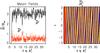 |
Fig. 1 Time series for a dominantly α2Ω dynamo with
ReM = 20, PrM = 5,
S = 0.1 and kf ≈ 3.1 (corresponding
to Run H of Table 3). Left:
rms value of
|


3. Model and methods
3.1. Numerical setup
We have run simulations of helically forced sheared turbulence in homogeneous isothermal
triply (shear) periodic cubic domains with sides of length 2π. The box
wavenumber, which is also the wavenumber of the observed mean fields, is therefore
k1 = 1. Unless otherwise specified, our simulations have
643 grid points. For the shear flow we have taken the one defined by (6). We solve the non-dimensionalized system
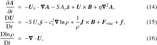 where
U is the fluid velocity excluding the shear flow,
where
U is the fluid velocity excluding the shear flow,
 is the advective
derivative, cs = 1 is the isothermal sound speed,
ρ the density,
is the advective
derivative, cs = 1 is the isothermal sound speed,
ρ the density, 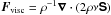 the viscous force,
 is the rate of strain
tensor, ν is the kinematic viscosity and f
the forcing term. We use the Pencil Code3, which employs sixth-order explicit finite differences in space and a third
order accurate time stepping method. While our code allows full compressibility, the
simulations are only weakly compressible (small Mach number). As in earlier work (Brandenburg 2001), in each time step the forcing
function is a snapshot of a circularly polarized plane wave. All these waves have the same
handedness, but their direction and phase change randomly from one time step to the next.
This forcing provides kinetic helicity. The nondimensional forcing amplitude,
f0 (see Haugen et al.
2004, for details), is arranged such that the Mach number associated with the
turbulent rms velocity is of the order of 0.1. In practice, this means that
f0 is in the range 0.02 to 0.05. The wavevectors are taken
from the set of vectors that satisfy periodicity and whose moduli are adequately close to
the target forcing wavenumber kf.
is the rate of strain
tensor, ν is the kinematic viscosity and f
the forcing term. We use the Pencil Code3, which employs sixth-order explicit finite differences in space and a third
order accurate time stepping method. While our code allows full compressibility, the
simulations are only weakly compressible (small Mach number). As in earlier work (Brandenburg 2001), in each time step the forcing
function is a snapshot of a circularly polarized plane wave. All these waves have the same
handedness, but their direction and phase change randomly from one time step to the next.
This forcing provides kinetic helicity. The nondimensional forcing amplitude,
f0 (see Haugen et al.
2004, for details), is arranged such that the Mach number associated with the
turbulent rms velocity is of the order of 0.1. In practice, this means that
f0 is in the range 0.02 to 0.05. The wavevectors are taken
from the set of vectors that satisfy periodicity and whose moduli are adequately close to
the target forcing wavenumber kf.
The magnetic vector potential is initialized with a weak Gaussian random field, the
initial velocity is given by  and the initial
density is uniform. In Table 1 we have collected
the control parameters and some key derived quantities of the model. Two parameters of
note are the magnetic Reynolds and Prandtl numbers,
and the initial
density is uniform. In Table 1 we have collected
the control parameters and some key derived quantities of the model. Two parameters of
note are the magnetic Reynolds and Prandtl numbers,
 (17)To characterize the
turbulence, we provide values of α and ηt
which represent the corresponding tensors as described in Sect. 2. These were determined using the test-field method (see Sect. 3.2) with test-field wavevector
(17)To characterize the
turbulence, we provide values of α and ηt
which represent the corresponding tensors as described in Sect. 2. These were determined using the test-field method (see Sect. 3.2) with test-field wavevector
 or
or  .
.
Control and derived parameters.
For our purposes, we require the helical turbulence to be strong enough that the α2 dynamo can safely be excited. Accordingly, we guaranteed that in all our simulations, ReM is above the critical value (of the order of unity) for α2 dynamos in the corresponding shearless setup (Brandenburg 2009). Further, some of the transitions we will study require long simulation times due to their rarity, which constrains us to modest numerical resolutions. This in turn prevents our (explicit) numerical resistivity from being small, so the turbulent velocities must be reasonably large for the stated super-critical values of ReM. Choosing furthermore subsonic shear speeds, we are restricted to a modest region of parameter space. In light of these limitations we operate mostly in a PrM > 1 regime.
3.2. Test-field method
A fundamental difficulty in extracting the tensors αij and ηij from a numerical simulation of (14)–(16)is that (5)is under-determined. However, turbulent transport depends only on the velocity field, so “daughter” simulations of the induction equation, whose velocity fields are continuously copied from the main run, share the same tensors αij and ηij. It is therefore possible to lift the degeneracy by running an adequate number of daughter simulations with suitably chosen “test” mean fields. We employ this test-field method (TFM); for an in-depth overview see Schrinner et al. (2005, 2007) and Brandenburg et al. (2008a,b). Recently the original method has been extended to systems with rapidly evolving mean-fields, requiring a more complicated ansatz than Eq. (5)(Hubbard & Brandenburg 2009) and to the situation with magnetic background turbulence (Rheinhardt & Brandenburg 2010).
In addition to calculating turbulent tensors for planar averages as described in the
references above, we will be interested in tensors that depend both on x
and z (that is, are y-averages). For this, we generalize
(5)to
 (18)There are 27
tensor components (as
(18)There are 27
tensor components (as  ), so nine test-fields are
required, which we choose to be of the form
), so nine test-fields are
required, which we choose to be of the form
 (19)where
fq(x,z) is defined,
according to the choice of q, to be one of the following functions:
(19)where
fq(x,z) is defined,
according to the choice of q, to be one of the following functions:
 and
BT is, as standard for test-field methods, an arbitrary
amplitude factor. Although the wavenumber of the test fields is usually treated as a
varying parameter, we need here to consider only the single value
k1 because the fastest growing and also the saturated
dynamos in the simulations are dominated by this wavenumber, the smallest possible in our
periodic setup. As is often the case in applications of the test-field method, we will
occasionally be faced with unstable solutions of the test problems. We treat that
difficulty by periodically resetting the test solutions (see Hubbard et al. 2009). Since it takes a finite time for the stable parts
of the test solutions to reach their stationary values, and as this time is frequently
close to the required reset time, only limited windows in the time series of the data are
valid.
and
BT is, as standard for test-field methods, an arbitrary
amplitude factor. Although the wavenumber of the test fields is usually treated as a
varying parameter, we need here to consider only the single value
k1 because the fastest growing and also the saturated
dynamos in the simulations are dominated by this wavenumber, the smallest possible in our
periodic setup. As is often the case in applications of the test-field method, we will
occasionally be faced with unstable solutions of the test problems. We treat that
difficulty by periodically resetting the test solutions (see Hubbard et al. 2009). Since it takes a finite time for the stable parts
of the test solutions to reach their stationary values, and as this time is frequently
close to the required reset time, only limited windows in the time series of the data are
valid.
4. Kinematic regime
The fruits of the linear analysis of Sect. 2.1 are not
always clear in the kinematic regime of direct numerical simulations. Consider first a low
value of ReM ≈ 5, slightly above its supposed marginal values
for both the α2 and the α2Ω modes.
When starting with a Beltrami
 field as in
(10)with
kx = k1, the
initialized dynamo mode indeed starts to grow exponentially after a short adjustment stage.
Its corresponding sibling mode, that is, the α2Ω one, is fed via
fluctuations and after a certain delay starts to grow exponentially in turn. Even without
including memory effects, the estimated growth rates are in good agreement with those
obtained from the transport coefficients measured by the test-field method. Further, the
expected geometries of both modes can be identified satisfactorily. If instead one uses the
measured transport coefficients to generate an appropriate initial
α2Ω field whose geometry is described by (12)with
kz = k1, it
grows again at the right rate. Its α2 sibling, however, never
appears. Instead a
field follows
the α2Ω mode, albeit with an rms value one order of magnitude
lower: we interpret this as “enslavement” of the
field by the
growing α2Ω mode: i.e., much like in Sect. 6.3, the magnetic field of the α2Ω mode
forces
via turbulent
motions that can be represented by transport coefficients depending on both
x and z. Only the geometry of the
α2Ω mode can be safely identified, while the
field shows a
strong imprint of the forcing wavenumber, furthering the enslavement hypothesis.
field as in
(10)with
kx = k1, the
initialized dynamo mode indeed starts to grow exponentially after a short adjustment stage.
Its corresponding sibling mode, that is, the α2Ω one, is fed via
fluctuations and after a certain delay starts to grow exponentially in turn. Even without
including memory effects, the estimated growth rates are in good agreement with those
obtained from the transport coefficients measured by the test-field method. Further, the
expected geometries of both modes can be identified satisfactorily. If instead one uses the
measured transport coefficients to generate an appropriate initial
α2Ω field whose geometry is described by (12)with
kz = k1, it
grows again at the right rate. Its α2 sibling, however, never
appears. Instead a
field follows
the α2Ω mode, albeit with an rms value one order of magnitude
lower: we interpret this as “enslavement” of the
field by the
growing α2Ω mode: i.e., much like in Sect. 6.3, the magnetic field of the α2Ω mode
forces
via turbulent
motions that can be represented by transport coefficients depending on both
x and z. Only the geometry of the
α2Ω mode can be safely identified, while the
field shows a
strong imprint of the forcing wavenumber, furthering the enslavement hypothesis.
Even for higher ReM the kinematic picture should still be clear
in the shearless case, S = 0: when starting with random initial conditions
one expects all three (Beltrami) α2 modes possible in a box,
that is, with |k| = k1, to
grow at similar rates. In Fig. 2 we present time
series, a butterfly diagram and spatial cuts for Run A of Table 2 (ReM ≈ 37) along with its shearless
counterpart, where the spatial cuts show the mean fields during the kinematic regime. For
S = 0 all three fields
,
 and
and
 indeed appear
with similar amplitudes and grow at a rate extracted with the test-field method. Their
identification as Beltrami fields, however, is all but clear, see Fig. 2,
indeed appear
with similar amplitudes and grow at a rate extracted with the test-field method. Their
identification as Beltrami fields, however, is all but clear, see Fig. 2,
 in lower
panel. At least a strong
|k| = k1 harmonic is
detectable in each of these fields.
in lower
panel. At least a strong
|k| = k1 harmonic is
detectable in each of these fields.
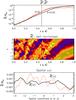 |
Fig. 2 Time series of the rms values of |


The sheared case is even more obscure. During the kinematic stage there are some
indications of a dynamo wave, albeit strongly entangled by fluctuating fields, see
Fig. 2, middle panel. More worrying however, the
growth rates and amplitudes of the and
fields are
very similar and no pronounced features of a Beltrami field can be found in
. The spatial
structure of the field,
expected to be characterized by
kz = k1, is even
less clear in this respect than that of the field in the
shearless case. However, an identifiable dynamo wave is markedly visible after entering the
saturation stage where the growth rate of falls below
that of .
For an explanation we refer to the occurrence of a small-scale dynamo at the given values
of ReM and S, checked by integrating Eq. (4)with  . It dominates the linear stage
and we hypothesize that it “enslaves” the and
fields, and
is responsible for the ragged character of their geometries. The fact that with shear there
is slower growth than without (see Fig. 2, upper
panel), contradictory to the linear analysis, can perhaps be traced down to the reduction of
α by the growing magnetic turbulence, cf. the magnetokinetic contribution
to α of Rheinhardt & Brandenburg
(2010). After the saturation of the small-scale dynamo, the
α2Ω mode can establish itself on the now settled
MHD turbulence, whereas the α2 mode had perhaps not enough time
to take shape. In the shearless case, in contrast, the small-scale dynamo, if it exists at
all, has at least a much smaller growth rate and is hence less capable of influencing the
mean field growth. The appearance of a small-scale dynamo in this parameter range is
plausible in view of the results in Schekochihin et al.
(2005) and Käpylä et al. (2008), although
those works use different setups.
. It dominates the linear stage
and we hypothesize that it “enslaves” the and
fields, and
is responsible for the ragged character of their geometries. The fact that with shear there
is slower growth than without (see Fig. 2, upper
panel), contradictory to the linear analysis, can perhaps be traced down to the reduction of
α by the growing magnetic turbulence, cf. the magnetokinetic contribution
to α of Rheinhardt & Brandenburg
(2010). After the saturation of the small-scale dynamo, the
α2Ω mode can establish itself on the now settled
MHD turbulence, whereas the α2 mode had perhaps not enough time
to take shape. In the shearless case, in contrast, the small-scale dynamo, if it exists at
all, has at least a much smaller growth rate and is hence less capable of influencing the
mean field growth. The appearance of a small-scale dynamo in this parameter range is
plausible in view of the results in Schekochihin et al.
(2005) and Käpylä et al. (2008), although
those works use different setups.
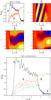 |
Fig. 3 Time series for Run A. Upper row: same quantities as in Fig. 1. Middle row:
|


5. Deterministic interactions of α2 and α2Ω modes
5.1. Numerical results
Here we report on the results of our simulations, a first set of which is characterized
in Table 2. In Fig. 3 we show time series for Run A, which saw a transition from a
z varying α2Ω dynamo
() to an
x varying α2 dynamo
(). As is
made clear in the bottom panel, there was a prolonged period where the two modes were
coexisting while their relative strengths were changing monotonically. However, note that
 is
stronger than , that
is, the α2 field is distorted during the transition. Run A was
repeated 16 times with the same parameters, but different random seeds, and all these runs
exhibited similar behavior. Likewise we performed runs where both the value of
η and the numerical resolution (cf. Runs B–D, I, J) were varied. As
these additional runs also showed the same transition pattern, we conclude that it is
deterministic for this level of shear and forcing. More, we conclude that for these cases
the α2Ω mode is unstable to the growth of an
α2 mode due to non-linear effects. Runs with the dynamical
parameters (S, urms) of Table 2 inevitably generate α2
fields from α2Ω fields after modest times, runs with
significantly different shear will usually (for most of the random seeds) exit the
kinematic regime into an α2Ω mode, and stay in that mode for a
prolonged time with no sign of an α2 field (but with random
transitions into the α2 mode, see Sect. 6).
is
stronger than , that
is, the α2 field is distorted during the transition. Run A was
repeated 16 times with the same parameters, but different random seeds, and all these runs
exhibited similar behavior. Likewise we performed runs where both the value of
η and the numerical resolution (cf. Runs B–D, I, J) were varied. As
these additional runs also showed the same transition pattern, we conclude that it is
deterministic for this level of shear and forcing. More, we conclude that for these cases
the α2Ω mode is unstable to the growth of an
α2 mode due to non-linear effects. Runs with the dynamical
parameters (S, urms) of Table 2 inevitably generate α2
fields from α2Ω fields after modest times, runs with
significantly different shear will usually (for most of the random seeds) exit the
kinematic regime into an α2Ω mode, and stay in that mode for a
prolonged time with no sign of an α2 field (but with random
transitions into the α2 mode, see Sect. 6).
Nonetheless all our simulation parameters allow runs to occasionally fail to fully enter the α2Ω regime, instead exiting the kinematic regime via a short transient α2Ω phase into the α2 mode, as shown in Fig. 4. One might speculate that this “weakness” of the α2Ω dynamo is due to strong fluctuations driven by powerful shear (compare the fluctuations of the α2Ω and α2 modes in Fig. 7) but the direct exit into the α2 mode has also been seen with lower shear as well. We emphasize that this “direct exit” seems to belong neither to the deterministic transitions discussed here nor to the random transitions discussed later.
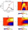 |
Fig. 4 Time series for a run with same parameters as Run J of Table 2, but different initial conditions, showing a transient, rather
than a quasi-stationary α2Ω regime. Top
left: rms values of |
Run parameters of deterministic transitions.
5.2. Analysis: mean-field approach
Clearly, the transition from the α2Ω mode to the
α2 one must be a consequence of the back-reaction of
onto
the flow. Within the mean-field picture, there are two channels available for it: (i) the
back-reaction onto the fluctuating flow, usually described as a dependence of
αij (more seldom
ηij) on the mean field and (ii) the
back-reaction onto to the mean flow by the mean Lorentz force, which might again be
decomposed into a part resulting from the fluctuating field,
 , and
one resulting from the mean field,
, and
one resulting from the mean field,  .
Here, we will deal with a flow generated by the latter force that straddles the
distinction of means and fluctuations: it survives under y-averaging, but
vanishes under the xy and yz averaging that reveals the
α2Ω and α2 dynamos respectively.
For simplicity we consider magnetic field configurations that would result from a
superposition of linear modes of the αΩ and
α2 dynamos, given in Eqs. (11) and (10)
respectively. Such a situation will inevitably occur during the kinematic growth phase if
both dynamos are supercritical, but is only relevant for analyzing the back-reaction onto
the flow if it at least to some extent continues into the non-linear regime. Our analysis
is linear in nature, so while it provides a qualitative framework for understanding the
transition process, it is surely not quantitatively accurate.
.
Here, we will deal with a flow generated by the latter force that straddles the
distinction of means and fluctuations: it survives under y-averaging, but
vanishes under the xy and yz averaging that reveals the
α2Ω and α2 dynamos respectively.
For simplicity we consider magnetic field configurations that would result from a
superposition of linear modes of the αΩ and
α2 dynamos, given in Eqs. (11) and (10)
respectively. Such a situation will inevitably occur during the kinematic growth phase if
both dynamos are supercritical, but is only relevant for analyzing the back-reaction onto
the flow if it at least to some extent continues into the non-linear regime. Our analysis
is linear in nature, so while it provides a qualitative framework for understanding the
transition process, it is surely not quantitatively accurate.
In order to be able to consider both and
as mean
fields under one and the same averaging, we have now to resort to y
averaging. Moreover, for the sake of clarity we will occasionally subject the resulting
x and z dependent mean fields further to spectral
filtering with respect to these coordinates. That is, we will consider only their first
harmonics
~eik1(x + z)
as mean fields.
Let us represent the mean field
⟨ B ⟩ y as superposition of
a
resembling the (x varying) α2 mode
 (Eq. (10)) and a
resembling the (z varying) αΩ mode
(Eq. (10)) and a
resembling the (z varying) αΩ mode
 (Eq. (11)):
 ![Mathematical equation: \begin{eqnarray} \label{mixedmodes} \BBZ &=&\BZ\left[ \begin{array}{c} \sin \,\zt\\ G\sin (\zt+\phi) \\ 0 \end{array} \right],\; \JJZ =k_1\BZ\left[ \begin{array}{c} -G \cos (\zt+\phi) \\ \cos \,\zt \\ 0 \end{array} \right], \nonumber \\[1mm] \BBX &=&\BX\left[ \begin{array}{c} 0 \\ H\sin \,\xk \\ \cos \,\xk \end{array} \right],\quad \JJX =k_1\BX\left[ \begin{array}{c} 0 \\ \sin \,\xk \\ H\cos \, \xk \end{array} \right], \end{eqnarray}](/articles/aa/full_html/2011/11/aa16705-11/aa16705-11-eq170.png) (20)with
z′ ≡ z − ct, recalling
that c is the speed of the dynamo wave (Eq. (12)). In the above,
π/4 ≤ φ ≤ 3π/4
and G,H,k1 > 0 are
appropriate for α > 0. The parameters
G and H capture the difference in the strengths of the
y and z components of
(20)with
z′ ≡ z − ct, recalling
that c is the speed of the dynamo wave (Eq. (12)). In the above,
π/4 ≤ φ ≤ 3π/4
and G,H,k1 > 0 are
appropriate for α > 0. The parameters
G and H capture the difference in the strengths of the
y and z components of
 or the
x or y components of
or the
x or y components of
 ,
respectively. We expect G > 1 as shear amplifies
the y component of an α2Ω mode well above its
x component. The inclusion of the parameter H, which
is unity for pure α2 modes will be justified below, see the
different strengths of
,
respectively. We expect G > 1 as shear amplifies
the y component of an α2Ω mode well above its
x component. The inclusion of the parameter H, which
is unity for pure α2 modes will be justified below, see the
different strengths of  and
and  in
Fig. 3, lower panel.
in
Fig. 3, lower panel.
The mean Lorentz force  for the superimposed fields can be written as
![Mathematical equation: \begin{eqnarray} \meanFF_L &=& \bra{\FF_L}_y \nonumber \\ &=&k_1\BX\BZ \cos \xk\, [\,G \cos (\zt+\phi) +H \sin \zt\,]\, \yyy +\nab \Phi. \end{eqnarray}](/articles/aa/full_html/2011/11/aa16705-11/aa16705-11-eq183.png) (21)As
the Mach numbers were found to be small throughout, we assume incompressibility and hence
drop the potential component ∇Φ. Further, we assume that
(21)As
the Mach numbers were found to be small throughout, we assume incompressibility and hence
drop the potential component ∇Φ. Further, we assume that
 and the mean velocity
driven by it are simply linked by a coefficient
and the mean velocity
driven by it are simply linked by a coefficient  , where the
total viscosity νT is the sum of the molecular
ν, and the turbulent viscosity νt. Thus we
can approximate the mean velocity due to the interaction of the superimposed mean fields
as
, where the
total viscosity νT is the sum of the molecular
ν, and the turbulent viscosity νt. Thus we
can approximate the mean velocity due to the interaction of the superimposed mean fields
as ![Mathematical equation: \begin{equation} \meanUU_L =U_L\cos\xk\left[\,G\cos(\zt+\phi)+H\sin \zt\,\right]\yyy, \label{Uquad} \end{equation}](/articles/aa/full_html/2011/11/aa16705-11/aa16705-11-eq189.png) (22)where
(22)where
 .
Clearly, this flow, having merely a y component, shows quadrupolar
geometry in the x − z plane as
.
Clearly, this flow, having merely a y component, shows quadrupolar
geometry in the x − z plane as
 can
be rewritten in the form
can
be rewritten in the form  with a
new amplitude and phase,
with a
new amplitude and phase,  and
φ′.
and
φ′.
The simulations show indeed a dominant part of that shape in the Lorentz-force generated
mean flow as can be seen from Fig. 5. There the
y averaged Uy is shown
together with its Fourier constituent
~eik1(x + z).
The latter contains approximately 10% of the energy in this component, or
 ,
indicating that the assumptions made in deriving (22)are reasonably well justified in a non-linear system.
,
indicating that the assumptions made in deriving (22)are reasonably well justified in a non-linear system.
Upon interaction with a or a
of the
form (20), the mean flow
 in (22)generates an
 and
and
 , respectively.
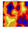 |
Fig. 5 ⟨ Uy ⟩ y for
Run A, taken at early time
(t = 1.45 tres) when
|
5.2.1. Dominating α2Ω mode
If  ,
then can be
treated as a perturbation, and we can drop higher order terms in
,
then can be
treated as a perturbation, and we can drop higher order terms in
 .
Accordingly, the z-averaged EMF due to the flow
is
.
Accordingly, the z-averaged EMF due to the flow
is
 (23)The curl of this EMF is
 (24)If
Gsinφ > H,
then I > 0 and for
H > 0 this EMF reinforces
(24)If
Gsinφ > H,
then I > 0 and for
H > 0 this EMF reinforces
 . Thus we see that the
inclusion of the parameter H in the ansatz for
,
Eq. (20), was justified as
receives enhanced forcing in comparison to .
. Thus we see that the
inclusion of the parameter H in the ansatz for
,
Eq. (20), was justified as
receives enhanced forcing in comparison to .
5.2.2. Dominating α2 mode
If  then we can in turn treat as a
perturbation. Further, as the system is dominated by the α2
mode, we will have H ~ 1. In this case we find
then we can in turn treat as a
perturbation. Further, as the system is dominated by the α2
mode, we will have H ~ 1. In this case we find
![Mathematical equation: \begin{eqnarray} \meanEMFZ &=&\:\bra{\meanUU_L \times \BBX}_x \\ &=&\:\frac{Kk_1}{2}\BZ {\BX}^2\left[\,G\cos(\zt+\phi)+H\sin \zt\,\right]\xxx, \nonumber \end{eqnarray}](/articles/aa/full_html/2011/11/aa16705-11/aa16705-11-eq217.png) (25)and
(25)and
![Mathematical equation: \begin{equation} \nab \times \meanEMFZ=\BZ\,\frac{K k_1^2 }{2}{\BX}^2\!\left[\,H\cos \zt-G\sin(\zt+\phi)\,\right]\yyy. \end{equation}](/articles/aa/full_html/2011/11/aa16705-11/aa16705-11-eq218.png) (26)We can write
(26)We can write
![Mathematical equation: \begin{eqnarray} &&H\cos \zt-G\sin(\zt+\phi)= \label{AlpMF}\nonumber \\ &&\left[(H\sin\phi-G)\sin(\zt+\phi)\right]_1+\left[H\cos\phi\cos(\zt+\phi)\right]_2. \end{eqnarray}](/articles/aa/full_html/2011/11/aa16705-11/aa16705-11-eq219.png) (27)If
Hsinφ − G < 0,
as expected since H ≈ 1,
G > 1, term [] 1 in (27)will act to damp
(27)If
Hsinφ − G < 0,
as expected since H ≈ 1,
G > 1, term [] 1 in (27)will act to damp
 , that
is, the perturbative α2Ω wave. Further, term
[] 2 is opposite in sign to the time-derivative of such a wave, so it
slows or reverses the direction of wave-propagation.
, that
is, the perturbative α2Ω wave. Further, term
[] 2 is opposite in sign to the time-derivative of such a wave, so it
slows or reverses the direction of wave-propagation.
5.2.3. Mean-field evolution
Here we assume again domination of the α2Ω mode, that is,
.
With Eqs. (7)and (24)the eigenvalue problem for the modified
α2 field is then
(adopting kx =
k1, kz = 0)
![Mathematical equation: \begin{equation} \lambda^X\BBX= \left[\begin{array}{ccc} -\eta_T k_1^2 & 0 & 0 \\ S & -\eta_T k_1^2 & -{\it i}(\alpha k_1+I) \\ 0 & i\alpha k_1 & -\eta_T k_1^2 \end{array}\right] \BBX, \end{equation}](/articles/aa/full_html/2011/11/aa16705-11/aa16705-11-eq226.png) (28)with eigenvalues
(28)with eigenvalues
 (29)Making the
approximation I ≫ αk1,
similar to the αΩ approximation
S ≫ αk1, we find
(29)Making the
approximation I ≫ αk1,
similar to the αΩ approximation
S ≫ αk1, we find
 (30)The above should be
compared with the growth rate of the αΩ dynamo,
λαΩ from (13)which is not touched by the occurrence of I. The
αΩ dynamo saturates when α has been quenched such
that the product αS settles at the marginal value
(30)The above should be
compared with the growth rate of the αΩ dynamo,
λαΩ from (13)which is not touched by the occurrence of I. The
αΩ dynamo saturates when α has been quenched such
that the product αS settles at the marginal value
 . If the
parameter I becomes comparable with the shear, i.e.,
I ~ S, then might
grow even when the α2Ω field is saturated, i.e.
. If the
parameter I becomes comparable with the shear, i.e.,
I ~ S, then might
grow even when the α2Ω field is saturated, i.e.
 . In other terms, the
saturated α2Ω mode is unstable to the growth of a
fratricidal α2 field, so the transition
will take a well defined time from the onset of the non-linear stage, determined by
λX.
. In other terms, the
saturated α2Ω mode is unstable to the growth of a
fratricidal α2 field, so the transition
will take a well defined time from the onset of the non-linear stage, determined by
λX.
We test this theory for Run A at the time of Fig. 5, t = 1.45tres, extracting
G and H from the relative strengths of the
x and y or y and z
components of the mean fields or
,
respectively, after a projection onto the first harmonics; see Eq. (20). The parameter I is
calculated from the magnetic and velocity fields using
 (31)with
 ,
where is the
amplitude of the quadrupolar constituent of the velocity field seen in Fig. 5. We find
,
where is the
amplitude of the quadrupolar constituent of the velocity field seen in Fig. 5. We find  ,
H ≃ 2.9, G ≃ 4.9, I ≃ 0.09, and
confirm that φ ≃ π/4. As
I > S = 0.05, the growth of
the x varying mode even when the α2Ω mode
is saturated is not surprising. Repeating this run16 times with different random seeds
(keeping the control parameters fixed) changed the occurrence time of the transition by
only one resistive time, suggesting that the transition is an essentially deterministic
process.
,
H ≃ 2.9, G ≃ 4.9, I ≃ 0.09, and
confirm that φ ≃ π/4. As
I > S = 0.05, the growth of
the x varying mode even when the α2Ω mode
is saturated is not surprising. Repeating this run16 times with different random seeds
(keeping the control parameters fixed) changed the occurrence time of the transition by
only one resistive time, suggesting that the transition is an essentially deterministic
process.
We have never seen a reverse transition from the α2 state back to the α2Ω state. This may be understood in terms of interacting modes, with the α2Ω mode being suppressed once the α2 mode is dominating; see Sect. 5.2.2.
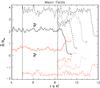 |
Fig. 6 Time series for Run F (solid lines), with rms values of
|
Run parameters for random transitions.
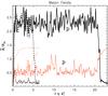 |
Fig. 7 Time series of Run G (solid, thick) along with a sibling run (dashed) with different seeds, showing significant differences in the transition start time. Dash-dotted: a run which never entered the α2Ω regime. Colors as in Fig. 6. |
6. Random transitions
6.1. Non-interacting modes
Not all transitions fit into the above deterministic picture of interacting
α2Ω and α2 modes. The behavior
above and below the shear value S = −0.05 that applies to the runs in
the previous section is qualitatively different. In Fig. 6 we present a set of time series of the rms values of
and
, all
related to Run F of Table 3. Secondary runs were
performed by branching off from the original simulation either at
t = 5tres, when the
α2Ω mode is well established and stationary, or at
t = 8.25tres, immediately before the
transition to the α2 mode in the primary run is launched. The
only difference between all these runs is in the random seed, which is used by the forcing
algorithm. In all, the time until the transition starts varies by
≈ 2.5tres, and many more turbulent turnover times
( turbulent turnover times per resistive time). The time elapsed during a transition is
always of the order of tres/2, unlike
3tres for the process seen in Fig. 3. Thus it is suggestive to assume that there might be a very slow,
still essentially deterministic process, preparing the transition, which is likely
resistive in nature as that is the longest obvious “native” timescale of the system. Slow
resistive effects are known to exist in dynamos, for example the slow resistive growth of
α2 dynamos in periodic systems. However, transitions can
indeed occur at very different times including the extreme case in which a run never
develops a quasi-stationary α2Ω mode, but instead enters the
α2 state almost immediately after the end of the kinematic
phase, see Fig. 7 (run G of Table 3). We believe therefore that under certain
circumstances the transition process is not a deterministic one, in that it is impossible
to predict or at least estimate the time until the transition. Figure 8 is a synopsis of simulations that belong to that type, hence do not
show the instability discussed in Sect. 5. Note that,
while corresponding setups without shear are known to enable
α2 modes for the entire ReM
range studied (Brandenburg 2009), we cannot rule out
that the α2 mode is sub-critical for
ReM = 10,S = −0.1 (i.e., it is possible
that the run denoted by the bottom left diamond in the upper panel did not transition
because it simply could not).
turbulent turnover times per resistive time). The time elapsed during a transition is
always of the order of tres/2, unlike
3tres for the process seen in Fig. 3. Thus it is suggestive to assume that there might be a very slow,
still essentially deterministic process, preparing the transition, which is likely
resistive in nature as that is the longest obvious “native” timescale of the system. Slow
resistive effects are known to exist in dynamos, for example the slow resistive growth of
α2 dynamos in periodic systems. However, transitions can
indeed occur at very different times including the extreme case in which a run never
develops a quasi-stationary α2Ω mode, but instead enters the
α2 state almost immediately after the end of the kinematic
phase, see Fig. 7 (run G of Table 3). We believe therefore that under certain
circumstances the transition process is not a deterministic one, in that it is impossible
to predict or at least estimate the time until the transition. Figure 8 is a synopsis of simulations that belong to that type, hence do not
show the instability discussed in Sect. 5. Note that,
while corresponding setups without shear are known to enable
α2 modes for the entire ReM
range studied (Brandenburg 2009), we cannot rule out
that the α2 mode is sub-critical for
ReM = 10,S = −0.1 (i.e., it is possible
that the run denoted by the bottom left diamond in the upper panel did not transition
because it simply could not).
The picture of random transitions is different from the interacting mode one of
Sect. 5 in several interesting ways. Crucially, the
α2Ω mode is here at least meta-stable against growth of the
α2 mode, as evinced by its prolonged life-time (hundreds of
turbulent times) and the small magnitude of , which
further is not dominated by an α2 mode. A reasonable working
hypothesis for the cases of Sect. 5 is then that,
there, the α2 mode is the only stable solution and, as soon as
the nonlinear stage has been entered, it starts to devour the
α2Ω one, settling after a time which is related to basic
parameters of the system and hence not random. In contrast, for the cases considered here,
we conclude that both the α2and the
α2Ω solutions are indeed stable (not only metastable) and
the latter has a well extended basin of entrainment. Due to its higher growth rate the
system settles first in the α2Ω mode and suppresses the
α2 mode efficiently. A transition to the latter can only
occur if a random fluctuation in the forcing is strong enough to push the system over the
separatrix into the basin of entrainment of the α2 mode. This
may happen after only a long time or even never during a simulation’s run time, cf.
diamond and square symbols, respectively, in Fig. 8,
see also the absence of a transition in Fig. 1 where
S = −0.1, ReM = 20. From these data one
can also derive that the tendency to leave the α2Ω state by a
random transition increases both with growing shear and ReM
(note the corresponding reduction in the blue squares’ size = time until transition in
Fig. 8). Although one would expect the basin of
entrainment of the α2Ω mode to enlarge with growing
S, it is conceivable that at the same time the level of velocity
fluctuations is raised, making transitions eventually more likely. Growing
ReM can readily be thought of increasing the fluctuation
level and hence the transition probability likewise. As already mentioned in Sect. 5, we see in addition “direct exits” from the kinematic
stage into a saturated α2 dynamo; see Fig. 8 (cross symbols) and Fig. 9.
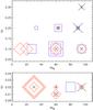 |
Fig. 8 Synopsis of runs which did not exhibit the instability discussed in Sect. 5. Crosses/black: a significant α2Ω mode was never developed (cf. Fig. 4), symbol size indicates the corresponding number of runs (1, 2 or 3). Square/blue: a transition occurred, size represents the time until transition (4 to 25tres). Diamond/red: the α2Ω stage was entered, but no transition occurred. Size represents the time span of simulation (5 to 35tres). Runs at the same position differ only in random seeds. Upper panel: high-shear runs, see Table 3 for those exhibiting a random transition. Lower panel: low-shear runs. Symbols scaled down by a factor of 3 with respect to upper panel. All runs in the lower panel had f0 = 0.04. |
Given that the examples for the first scenario (Table 2) differ from those for the second (Table 3) mainly in their lower rate of shear, our conclusion seems reasonable as stronger shear should result in a clearer preference of the α2Ω mode because the α2 mode does not feel the shear. Or, in other terms, from a certain shear rate S on, the α2Ω mode should acquire a basin of entrainment with a finite “volume” that grows with S. If this picture is true, transitions in the two scenarios should have clearly different characteristics, and indeed, the transition in Fig. 6 is markedly faster than that seen in Fig. 3.
Once the shear rate is dropped markedly below S = 0.05, the typical
value for deterministic transitions, the system again seems to settle in
a domain similar to the high-shear ( ) one,
namely one with both the α2 and the
α2Ω modes being stable. However, entering into the
α2 state immediately after the kinematic stage (the “direct
exit”) appears now to be more likely, while at the same time random transitions away from
a settled α2Ω state become extremely rare:
Over a run time of 3 × 10³ tres accumulated over
several runs with S = 0.01,0.02 as well as target values
of ReM around 30, 60, and 90, only one transition was observed
(for
ReM = 80,PrM = 5,
S = 0.02, after 8 × 10² tres);
see also Fig. 8, lower panel. Plausibility arguments
for the occurrence of this “low shear” domain, in particular for the apparent regaining of
a finite basin of entrainment by the α2Ω mode which has to be
implied, are not in sight.
) one,
namely one with both the α2 and the
α2Ω modes being stable. However, entering into the
α2 state immediately after the kinematic stage (the “direct
exit”) appears now to be more likely, while at the same time random transitions away from
a settled α2Ω state become extremely rare:
Over a run time of 3 × 10³ tres accumulated over
several runs with S = 0.01,0.02 as well as target values
of ReM around 30, 60, and 90, only one transition was observed
(for
ReM = 80,PrM = 5,
S = 0.02, after 8 × 10² tres);
see also Fig. 8, lower panel. Plausibility arguments
for the occurrence of this “low shear” domain, in particular for the apparent regaining of
a finite basin of entrainment by the α2Ω mode which has to be
implied, are not in sight.
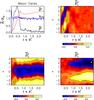 |
Fig. 9 Time series for Run E of Table 3 showing a transient, not a stationary α2Ω regime. For explanations see Fig. 4. Note the considerably faster growth of the α2Ω mode during the kinematic phase and the lack of a well defined phase with a dominating, but declining α2Ω mode. |
As in the transitions discussed in Sect. 5, we have not here seen the α2 mode transition back into the α2Ω mode. Some attempts were made to provoke this reverse transition by perturbing the α2 state with a (sufficiently strong) α2Ω mode. While in some runs it indeed took over, velocities were attained for which the numerics are unreliable, and often proved numerically unstable, making the results inconclusive. However, such a behavior is not entirely surprising as the α2Ω saturation process can anyway be somewhat wild, cf. Fig. 4.
The absence of spontaneous reverse transitions appears plausible insofar the time variability of the α2 mode is much smaller than that of the α2Ω mode, which can clearly be seen in Fig. 10 for Run H. That is, events capable of pushing the system over the separatrix are simply much rarer. Significantly longer integration times are likely needed for their eventual detection, but it is also conceivable that the triggering event never shows up.
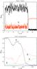 |
Fig. 10 Time series of Run H. Upper panel: rms values of
|

6.2. Large scale patterns
Run H will be examined here in more detail. Curiously,
⟨ Uy ⟩ y
taken just during the transition as shown in Fig. 11
does not show the quadrupolar pattern of Fig. 5. It
is therefore not surprising that the butterfly diagrams in Fig. 12 do not show a direct transition from the
α2Ω to the α2 dynamo, as
develops
significantly later than . This is
clearly visible in Fig. 10, lower panel. As
consideration of the mean flow due to the Lorentz force of the mean field alone is
obviously not fruitful in explaining this transition, we recall that the back-reaction of
the mean field onto the turbulence opens another channel of nonlinear interaction.
According to elementary mean-field dynamo theory, the α effect is caused by the helicity in the flow: α ~ ⟨ w·u ⟩ , where w ≡ ∇ × u is the fluctuating vorticity. Further, the back-reaction of the mean field on the turbulence, which saturates the dynamo, is assumed to be captured by the current helicity ⟨ j·b ⟩ . It is often related to the magnetic helicity ⟨ a·b ⟩ and thought to reduce the original α by producing a magnetic contribution of opposite sign. In Fig. 13 we present time-series of the power spectra of these helicity correlators across the transition. However, we see no clear signal around the transition event.
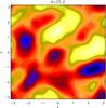 |
Fig. 11 ⟨ Uy ⟩ y taken during the transition of Run H shown in Fig. 10 (t = 25.2tres). Note the lack of a quadrupolar geometry. |
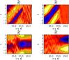 |
Fig. 12 Butterfly diagrams for Run H (see Fig. 10).
Note that |
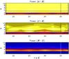 |
Fig. 13 Time series of the helicity power spectra for Run H. Horizontal line: forcing wavenumber kf ≈ 3.1. Vertical line: border between low-resolution observations (every 0.5tres) for t < 25tres and higher-resolution observations (every 0.1tres ) for t > 25tres. Possible features in the latter range are likely due to the increased temporal resolution. |
6.3. Mean-field analysis with y averaging
To examine the problem more closely, we recall Eq. (18) for a mean defined by the y average:
 (32)It is clear that the
Fourier constituents of αij and
ηijk with wavenumber
k1 in both x and z (the
quadrupolar constituents) can create an EMF
(32)It is clear that the
Fourier constituents of αij and
ηijk with wavenumber
k1 in both x and z (the
quadrupolar constituents) can create an EMF  out of a field , both
with the same wavenumber:
out of a field , both
with the same wavenumber: 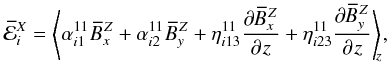 (33)where
the superscripts indicate the coefficients to be the Fourier constituents
~eik1(x + y)
and
(33)where
the superscripts indicate the coefficients to be the Fourier constituents
~eik1(x + y)
and  is
assumed to vanish. Note that each of them is actually given by four values, e.g., the two
amplitudes and phases in:
is
assumed to vanish. Note that each of them is actually given by four values, e.g., the two
amplitudes and phases in:  (34)The coefficients
relevant for the generation of (from
(34)The coefficients
relevant for the generation of (from
 alone) are
 and
and
 . We have
used the test-field method (see Sect. 3.2) to find
them and present the results in Fig. 14. They turn
out to be surprisingly large, when compared to the rms velocity (e.g.,
. We have
used the test-field method (see Sect. 3.2) to find
them and present the results in Fig. 14. They turn
out to be surprisingly large, when compared to the rms velocity (e.g.,
 ) and some may show
a trend across the transition from the α2Ω to the
α2 field. This overall trend is hypothesized to be due to
the increase in urms that accompanies the transition from a
stronger α2Ω field to a weaker α2
field with less potential to inhibit the flow. It is interesting that the large transport
coefficients (ignoring
) and some may show
a trend across the transition from the α2Ω to the
α2 field. This overall trend is hypothesized to be due to
the increase in urms that accompanies the transition from a
stronger α2Ω field to a weaker α2
field with less potential to inhibit the flow. It is interesting that the large transport
coefficients (ignoring  and
and
 which are
without effect) are all those which generate an out
of
which are
without effect) are all those which generate an out
of  , i.e.,
out of the component that feels the effect of shear. We speculate that these coefficients
feel the shear quite strongly.
, i.e.,
out of the component that feels the effect of shear. We speculate that these coefficients
feel the shear quite strongly.
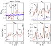 |
Fig. 14 Run H. Upper left panel: rms values of
|


7. Discussion and conclusions
We have demonstrated that, while α2Ω modes are kinematically preferred to α2 modes in homogeneous systems that support both, the α2 mode acts in a fratricidal manner against the former after the nonlinear stage has been reached. This transition can occur in at least two different fashions. Further, we have not observed the reverse process. One of the two transition processes, based on superposed α2Ω and α2 modes, operates in a basically deterministic fashion through a large-scale velocity pattern generated by the interaction of the modes. In contrast, we interpret the mechanism of the second process, which may start only many resistive times past the saturation of the α2Ω dynamo, by assuming that both the α2Ω and the α2 modes are stable solutions of the nonlinear system. Transitions occur if due to the random forcing a sufficiently strong perturbation builds up which tosses the system out of the basin of entrainment of the α2Ω mode into that of the α2 mode. This hypothesis is bolstered by both the random timing of these transitions and by the large time-variability seen in the amplitude of the α2Ω field. A return seems to be much less likely as the level of fluctuations of the α2 mode is, by contrast, greatly reduced. Random transitions are influenced by the shear rate. Above the shear level of S = 0.05 associated with deterministic transitions, eventual random transitions appear to be inevitable. Markedly below that level they are, at best, extremely rare. This suggests strongly that the vulnerability of an α2Ω mode to transitions increases with its dynamo number.
These results fit with earlier work studying dynamos whose non-linear behavior is fundamentally different from their linear one (e.g., Fuchs et al. 1999). While our simulations are limited to Cartesian, cubic, shearing-periodic domains, they are particularly exciting given that the only dynamo which has been observed over a long baseline and which could be either α2Ω or α2 , the solar dynamo, indeed shows differing modes of operation (regular cycles vs. deep minima). The results are also disturbing in that we have evidence for non-deterministic, rare (as they occur on scales of multiple resistive times or hundreds of turbulent turnovers) mode changes that show no evidence for a return. While a bifurcation between different stable modes has long been an acknowledged possibility for dynamos (Brandenburg et al. 1989; Jennings 1991; Covas & Tavakol 1997), a rare, stochastic, possibly uni-directional transition is perhaps the most troublesome consequence of such bifurcations except for the ultimate self-extinction.
Given that the mean-field transport coefficients have been systematically derived for many of the runs, it may sound plausible to study the nonlinear stability of different dynamo regimes by means of mean field models. This would allow to construct a stability map for the system to test the hypothesis made in the paper. However, there are two difficulties: firstly, the derived transport coefficients apply only for the specific mean field for which they have been calculated, i.e. they are not the functional derivatives of the mean EMF with respect to the mean field or current density and to our knowledge the technology to do better does not yet exist. This deficiency applies only to the non-linear regime, of course. Secondly, to overcome this restriction one could assume that the transport coefficients are smooth functionals of the mean field and so can be obtained from a finite set of data points by interpolation. This would require only to perturb the system into neighboring states, from which, however, it would tend to return to the original state in a self-regulated way. As the transport coefficients can only be calculated for sufficiently slowly changing flows, the set of obtainable data points would be strongly limited.
The αΩ dynamo is believed to be common and important for systems like the Sun or accretion disks, which all have long life-times compared to turbulent turnover times. It is then a daunting possibility that we could be forced to stretch our simulations over very long temporal base-lines to find the actual long-lasting field configuration. More positively, our result, while in a different geometry, increases the importance of recent work on non-oscillatory αΩ and oscillatory α2 modes in spherical shells for the solar dynamo (Mitra et al. 2010; Schrinner et al. 2011).
Strictly speaking, shear could introduce anisotropy felt by mean fields with non-vanishing z-components. Our results do not reveal any such.
When assuming both kx and
kz to be different from zero, but keeping
the αΩ approximation valid and
kz fixed, the phase speed of the dynamo
wave does not change while the growth rate is reduced by
 . However,
the eigenmode has now a z component ~
. However,
the eigenmode has now a z component ~
 . Such modes were not
observed in our simulations.
. Such modes were not
observed in our simulations.
Acknowledgments
We thank the anonymous referee for having made detailed suggestions that have helped improving the clarity of the paper. We acknowledge the allocation of computing resources provided by the Swedish National Allocations Committee at the Center for Parallel Computers at the Royal Institute of Technology in Stockholm and the National Supercomputer Centers in Linköping. This work was supported in part by the European Research Council under the AstroDyn Research Project No. 227952 and the Swedish Research Council Grant No. 621-2007-4064.
References
- Baryshnikova, I., & Shukurov, A. 1987, Astron. Nachr., 308, 89 [NASA ADS] [CrossRef] [Google Scholar]
- Brandenburg, A. 2001, ApJ, 550, 824 [NASA ADS] [CrossRef] [Google Scholar]
- Brandenburg, A. 2009, ApJ, 697, 1206 [NASA ADS] [CrossRef] [Google Scholar]
- Brandenburg, A., & Subramanian, K. 2005, Phys. Rep., 417, 1 [NASA ADS] [CrossRef] [Google Scholar]
- Brandenburg, A., Krause, F., Meinel, R., Moss, D., & Tuominen, I. 1989, A&A, 213, 411 [NASA ADS] [Google Scholar]
- Brandenburg, A., Rädler, K.-H., & Schrinner, M. 2008a, A&A, 482, 739 [NASA ADS] [CrossRef] [EDP Sciences] [Google Scholar]
- Brandenburg, A., Rädler, K.-H., Rheinhardt, M., & Käpylä, P. J. 2008b, ApJ, 676, 740 [NASA ADS] [CrossRef] [Google Scholar]
- Charbonneau, P. 2010, Liv. Rev. Sol. Phys., 7, 3 [Google Scholar]
- Covas, E., Ashwin, P., & Tavakol, R. 1997, Phys. Rev. E, 56, 6451 [NASA ADS] [CrossRef] [Google Scholar]
- Christensen, U., Olson, P., & Glatzmaier, G. A. 1999, Geophys. J. Int., 138, 393 [NASA ADS] [CrossRef] [Google Scholar]
- Covas, E., & Tavakol, R. 1997, Phys. Rev. E, 55, 6641 [NASA ADS] [CrossRef] [Google Scholar]
- Eddy, J. A. 1976, Science, 286, 1198 [Google Scholar]
- Fuchs, H., Rädler, K.-H., & Rheinhardt, M. 1999, Astron. Nachr., 320, 129 [NASA ADS] [CrossRef] [Google Scholar]
- Grote, E., & Busse, F. 2000, Phys. Rev. E, 62, 4457 [Google Scholar]
- Haugen, N. E. L., Brandenburg, A., & Dobler, W. 2004, Phys. Rev. E, 70, 016308 [NASA ADS] [CrossRef] [Google Scholar]
- Hubbard, A., & Brandenburg, A. 2009, ApJ, 706, 712 [NASA ADS] [CrossRef] [Google Scholar]
- Hubbard, A., Del Sordo, F., Käpylä, P. J., & Brandenburg, A. 2009, MNRAS, 398, 1891 [NASA ADS] [CrossRef] [Google Scholar]
- Jennings, R. L. 1991, Geophys. Astrophys. Fluid Dyn., 57, 147 [NASA ADS] [CrossRef] [Google Scholar]
- Käpylä, P. J., & Brandenburg, A. 2009, ApJ, 699, 1059 [NASA ADS] [CrossRef] [Google Scholar]
- Käpylä, P. J., Korpi, M. J., & Brandenburg, A. 2008, A&A, 491, 353 [NASA ADS] [CrossRef] [EDP Sciences] [Google Scholar]
- Mitra, D., Tavakol, R., Käpylä, P. J., & Brandenburg, A. 2010, ApJ, 719, L1 [NASA ADS] [CrossRef] [Google Scholar]
- Rädler, K.-H., & Bräuer, H.-J. 1987, Astron. Nachr., 308, 101 [NASA ADS] [CrossRef] [Google Scholar]
- Rädler, K.-H., Wiedemann, E., Brandenburg, A., Meinel, R., & Tuominen, I. 1990, A&A, 239, 413 [NASA ADS] [Google Scholar]
- Rheinhardt, M., & Brandenburg, A. 2010, A&A, 520, A28 [NASA ADS] [CrossRef] [EDP Sciences] [Google Scholar]
- Schekochihin, A. A., Haugen, N. E. L., Brandenburg, A., et al. 2005, ApJ, 625, L115 [NASA ADS] [CrossRef] [Google Scholar]
- Schrinner, M., Rädler, K.-H., Schmitt, D., Rheinhardt, M., & Christensen, U. 2005, Astron. Nachr., 326, 245 [NASA ADS] [CrossRef] [Google Scholar]
- Schrinner, M., Rädler, K.-H., Schmitt, D., Rheinhardt, M., & Christensen, U. R. 2007, Geophys. Astrophys. Fluid Dyn., 101, 81 [NASA ADS] [CrossRef] [MathSciNet] [Google Scholar]
- Schrinner, M., Petitdemange, L., & Dormy, E. 2011, A&A, 530, A140 [NASA ADS] [CrossRef] [EDP Sciences] [Google Scholar]
- Steenbeck, M., & Krause, F. 1969, Astron. Nachr., 291, 49 [NASA ADS] [CrossRef] [Google Scholar]
- Stefani, F., & Gerbeth, G. 2003, Phys. Rev. E, 67, 027302 [NASA ADS] [CrossRef] [Google Scholar]
All Tables
All Figures
|
Fig. 1 Time series for a dominantly α2Ω dynamo with
ReM = 20, PrM = 5,
S = 0.1 and kf ≈ 3.1 (corresponding
to Run H of Table 3). Left:
rms value of
|
| In the text | |
|
Fig. 2 Time series of the rms values of |
| In the text | |
|
Fig. 3 Time series for Run A. Upper row: same quantities as in Fig. 1. Middle row:
|
| In the text | |
|
Fig. 4 Time series for a run with same parameters as Run J of Table 2, but different initial conditions, showing a transient, rather
than a quasi-stationary α2Ω regime. Top
left: rms values of |
| In the text | |
|
Fig. 5 ⟨ Uy ⟩ y for
Run A, taken at early time
(t = 1.45 tres) when
|
| In the text | |
|
Fig. 6 Time series for Run F (solid lines), with rms values of
|
| In the text | |
|
Fig. 7 Time series of Run G (solid, thick) along with a sibling run (dashed) with different seeds, showing significant differences in the transition start time. Dash-dotted: a run which never entered the α2Ω regime. Colors as in Fig. 6. |
| In the text | |
|
Fig. 8 Synopsis of runs which did not exhibit the instability discussed in Sect. 5. Crosses/black: a significant α2Ω mode was never developed (cf. Fig. 4), symbol size indicates the corresponding number of runs (1, 2 or 3). Square/blue: a transition occurred, size represents the time until transition (4 to 25tres). Diamond/red: the α2Ω stage was entered, but no transition occurred. Size represents the time span of simulation (5 to 35tres). Runs at the same position differ only in random seeds. Upper panel: high-shear runs, see Table 3 for those exhibiting a random transition. Lower panel: low-shear runs. Symbols scaled down by a factor of 3 with respect to upper panel. All runs in the lower panel had f0 = 0.04. |
| In the text | |
|
Fig. 9 Time series for Run E of Table 3 showing a transient, not a stationary α2Ω regime. For explanations see Fig. 4. Note the considerably faster growth of the α2Ω mode during the kinematic phase and the lack of a well defined phase with a dominating, but declining α2Ω mode. |
| In the text | |
|
Fig. 10 Time series of Run H. Upper panel: rms values of
|
| In the text | |
|
Fig. 11 ⟨ Uy ⟩ y taken during the transition of Run H shown in Fig. 10 (t = 25.2tres). Note the lack of a quadrupolar geometry. |
| In the text | |
|
Fig. 12 Butterfly diagrams for Run H (see Fig. 10).
Note that |
| In the text | |
|
Fig. 13 Time series of the helicity power spectra for Run H. Horizontal line: forcing wavenumber kf ≈ 3.1. Vertical line: border between low-resolution observations (every 0.5tres) for t < 25tres and higher-resolution observations (every 0.1tres ) for t > 25tres. Possible features in the latter range are likely due to the increased temporal resolution. |
| In the text | |
|
Fig. 14 Run H. Upper left panel: rms values of
|
| In the text | |
Current usage metrics show cumulative count of Article Views (full-text article views including HTML views, PDF and ePub downloads, according to the available data) and Abstracts Views on Vision4Press platform.
Data correspond to usage on the plateform after 2015. The current usage metrics is available 48-96 hours after online publication and is updated daily on week days.
Initial download of the metrics may take a while.