| Issue |
A&A
Volume 535, November 2011
|
|
|---|---|---|
| Article Number | A128 | |
| Number of page(s) | 17 | |
| Section | Galactic structure, stellar clusters and populations | |
| DOI | https://doi.org/10.1051/0004-6361/201116559 | |
| Published online | 02 December 2011 | |
Characterizing precursors to stellar clusters with Herschel⋆,⋆⋆
1
Center for Astrophysics and Space Astronomy, University of
Colorado, Boulder,
CO
80309, USA
e-mail: This email address is being protected from spambots. You need JavaScript enabled to view it.
2
Université de Toulouse (UPS-OMP), Institut de Recherche en Astrophysique et
Planétologie, France
3
CNRS, UMR 5277, 9 Av. colonel Roche, BP
44346, 31028
Toulouse Cedex 4,
France
4
School of Physics, University of Exeter,
Stocker Road, Exeter
EX4 4QL,
UK
5
Jodrell Bank Centre for Astrophysics, School of Physics and
Astronomy, University of Manchester, Manchester
M13 9PL,
UK
6
Canadian Institute for Theoretical Astrophysics, University of
Toronto, Toronto,
ON
M5S 3H8,
Canada
7
INAF-Instituto, Fisica Spazio Interplanetario, Via Fosso del Cavaliere 100, 00133
Roma,
Italy
8
Laboratoire AIM, CEA/DSM – INSU/CNRS – Université Paris Diderot,
IRFU/SAp CEA-Saclay, 91191
Gif-sur-Yvette,
France
9
INAF - Osservatorio Astrofisico di Arcetri,
Firenze,
Italy
10
European Southern Observatory, Garching bei Muenchen,
Germany
11
Centre for Astrophysics Research, Science and Technology Research
Institute, University of Hertfordshire, Hatfield, UK
Received:
22
January
2011
Accepted:
22
September
2011
Abstract
Context. Despite their profound effect on the universe, the formation of massive stars and stellar clusters remains elusive. Recent advances in observing facilities and computing power have brought us closer to understanding this formation process. In the past decade, compelling evidence has emerged that suggests infrared dark clouds (IRDCs) may be precursors to stellar clusters. However, the usual method for identifying IRDCs is biased by the requirement that they are seen in absorption against background mid-IR emission, whereas dust continuum observations allow cold, dense pre-stellar-clusters to be identified anywhere.
Aims. We aim to understand what dust temperatures and column densities characterize and distinguish IRDCs, to explore the population of dust continuum sources that are not IRDCs, and to roughly characterize the level of star formation activity in these dust continuum sources.
Methods. We use Hi-GAL 70 to 500 μm data to identify dust continuum sources in the ℓ = 30° and ℓ = 59° Hi-GAL science demonstration phase (SDP) fields, to characterize and subtract the Galactic cirrus emission, and perform pixel-by-pixel modified blackbody fits on cirrus-subtracted Hi-GAL sources. We utilize archival Spitzer data to indicate the level of star-forming activity in each pixel, from mid-IR-dark to mid-IR-bright.
Results. We present temperature and column density maps in the Hi-GAL ℓ = 30° and ℓ = 59° SDP fields, as well as a robust algorithm for cirrus subtraction and source identification using Hi-GAL data. We report on the fraction of Hi-GAL source pixels which are mid-IR-dark, mid-IR-neutral, or mid-IR-bright in both fields. We find significant trends in column density and temperature between mid-IR-dark and mid-IR-bright pixels; mid-IR-dark pixels are about 10 K colder and have a factor of 2 higher column density on average than mid-IR-bright pixels. We find that Hi-GAL dust continuum sources span a range of evolutionary states from pre- to star-forming, and that warmer sources are associated with more star formation tracers. Additionally, there is a trend of increasing temperature with tracer type from mid-IR-dark at the coldest, to outflow/maser sources in the middle, and finally to 8 and 24 μm bright sources at the warmest. Finally, we identify five candidate IRDC-like sources on the far-side of the Galaxy. These are cold (~20 K), high column density (N(H2) > 1022 cm-2) clouds identified with Hi-GAL which, despite bright surrounding mid-IR emission, show little to no absorption at 8 μm. These are the first inner Galaxy far-side candidate IRDCs of which the authors are aware.
Key words: stars: formation / dust, extinction / Galaxy: structure
Herschel in an ESA space observatory with science instruments provided by European-led Principal Investigator consortia and with important participation by NASA.
The FITS files discussed in the paper would be released publicly WITH the Hi-GAL data (on the Hi-GAL website) when the Hi-GAL data is released publicly.
© ESO, 2011
1. Introduction
Massive stars play a dominant role in shaping the Universe through their immense ionizing radiation, winds, and spectacular explosive death, yet their formation mechanism remains poorly understood. The dominant mode of star formation, and perhaps the only mode for massive star formation seems to be clustered (Lada & Lada 2003; de Wit et al. 2005). The definition of clustered can be called into question (e.g., Bressert et al. 2010; Gieles & Portegies Zwart 2011), but the search for young, massive star forming regions is still directed toward “proto-clusters”: cold, dense, massive molecular clumps. Galactic embedded clusters are characterized by high densities (n ~ 104−107 cm-3), radii of about 0.5−1 pc, temperatures of about 50−200 K, and masses around 102−103 M⊙ (Lada & Lada 2003; Motte et al. 2003). Proto-clusters represent a slightly earlier stage, before star formation has commenced, and so we expect the properties to be similar to those of the embedded clusters except that proto-clusters ought to be colder. We are most interested in searching for the more massive proto-clusters where massive stars may be forming, M ≳ 100 M⊙. Direct observation of proto-clusters is complicated: they are rare, and therefore further away on average than isolated low mass star-forming regions, proto-clusters have high column densities, meaning that the proto-stars are highly embedded, and massive stars evolve rapidly and quickly heat and ionize their surroundings, disrupting their natal molecular cloud.
Searches for proto-clusters or massive proto-stars are usually targeted at long-wavelengths, as dust continuum emission from these cold, dense sources peaks in the far-IR to sub-mm. Surveys of molecular lines are another approach for identifying potential proto-clusters, although these surveys may be time-intensive and interpreting molecular line spectra is complicated by excitation conditions and optical depth. The discovery of infrared dark clouds (IRDCs, Egan et al. 1998; Perault et al. 1996; Omont et al. 2003), opened a new window to viewing these cold, dense potential proto-clusters in silhouette against the bright Galactic mid-IR background. In the past decade, compelling evidence has emerged that suggests that some IRDCs may be precursors to massive stars and clusters (e.g., Rathborne et al. 2006; Ragan et al. 2006; Beuther & Sridharan 2007; Parsons et al. 2009; Battersby et al. 2010). While there exist many small IRDCs (e.g., Peretto & Fuller 2010; Kauffmann & Pillai 2010), the most massive ones (M ~ 103−4 M⊙, nH > 105 cm-3, T < 25 K, Rathborne et al. 2006; Egan et al. 1998; Carey et al. 1998) are consistent with expectations for a proto-cluster. However, the identification of an IRDC requires that it be on the near-side of a bright mid-IR background. This limits our potential to understand the Galactic distribution of potential proto-clusters.
Far-IR and submm dust continuum surveys are a powerful way to identify proto-clusters throughout the Galaxy, as the cold, dense dust is optically thin at these wavelengths. Surveys such as the Bolocam Galactic Plane Survey (BGPS, Aguirre et al. 2011) at 1.1 mm, the APEX Telescope Large Area Survey of the GALaxy (ATLASGAL, Schuller et al. 2009) at 870 μm, and now Herschel Infrared GALactic plane survey (Hi-GAL, Molinari et al. 2010a) from 70 to 500 μm are promising tools for understanding star cluster formation on a Galactic scale. However, the sources identified in these surveys may span a large range of evolutionary states, from pre-star-forming to star-forming, and further analysis or intercomparison may be necessary to identify the pre-star-forming regions. Since dust temperatures and column densities can be derived from the multi-wavelength Hi-GAL data, this data set allows for the distinction to be made between pre- and star-forming regions.
For this study, we utilize data from the Hi-GAL survey (Molinari et al. 2010a) from 70 to 500 μm in the ℓ = 30° and ℓ = 59° SDP fields to characterize dust continuum sources. We investigate differences in the physical properties of mid-IR-dark and mid-IR-bright clouds identified in the dust continuum, and also the physical properties of sources associated with various star formation tracers. We use extended green objects (EGOs, also known as “green fuzzies”, Cyganowski et al. 2008; Chambers et al. 2009) to trace outflows from young stars, CH3OH masers to trace sites of massive star formation, and 8 and 24 μm emission to indicate an accreting proto-star or UCHII Region (Battersby et al. 2010).
This paper is organized as follows. In Sect. 2 we introduce the Hi-GAL observing strategy and discuss archival data used in our analysis. In Sect. 3 we describe the Galactic cirrus emission removal and source identification methods, the modified blackbody fitting procedure, and how the star formation tracers were incorporated. Section 4 describes our results, including a discussion of uncertainties, the properties of the cirrus cloud emission, the temperature and column density maps, the association of Hi-GAL sources with mid-IR-dark and mid-IR-bright sources, and star formation tracers in Hi-GAL sources. In Sect. 5 we present five candidate IRDC-like clouds on the far-side of the Galaxy, and finally, in Sect. 6 we summarize our conclusions.
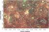 |
Fig. 1 A three-color GLIMPSE image with logarithmic BGPS 1.1 mm dust continuum contours (from 90 mJy to 0.8 Jy) on our test region in the Hi-GAL SDP ℓ = 30° field. Red: 8 μm, green: 4.5 μm, and blue: 3.6 μm. This figure demonstrates the distinction between the IRDC and dust continuum population. Some dust continuum sources are mid-IR-bright, some are mid-IR-dark, and some have no IR correlation. The object in the center is particularly well-suited as a test case for this study as it contains both mid-IR-bright and mid-IR-dark dust continuum sources radiating as filaments on either side of a young HII region complex. |
2. Observations and archival data
2.1. Hi-GAL
The Hi-GAL (Molinari et al. 2010a), is an Open Time Key Project of the Herschel Space Observatory (Pilbratt et al. 2010). Hi-GAL will perform a 5-band photometric survey of the Galactic plane in a |b| ≤ 1°-wide strip from −70° ≤ ℓ ≤ 70° at 70, 160, 250, 350, and 500 μm using the PACS (Poglitsch et al. 2010) and SPIRE (Griffin et al. 2010) imaging cameras in parallel mode. Two 2° × 2° regions of the Hi-GAL survey were completed during the science demonstration phase (SDP; Molinari et al. 2010a), centered at approximately [ℓ, b] = [30°, 0°] and [59°, 0°].
Data reduction was carried out using the Herschel interactive processing environment (HIPE, Ott 2011) with custom reduction scripts that deviated considerably from the standard processing for PACS (Poglitsch et al. 2010), and to a lesser extent for SPIRE (Griffin et al. 2010). A detailed description of the entire data reduction procedure can be found in Traficante et al. (2011).
The zero-level offsets in the Herschel maps were established by comparison with the IRAS and Planck data at comparable wavelengths, following the same procedure as described in Bernard et al. (2010). We compared the Herschel-SPIRE and PACS data with the predictions of a model provided by the Planck collaboration (Planck Core-Team, priv. comm.) and constrained on the Planck and IRIS data (Miville-Deschênes & Lagache 2005). The model uses the all-sky dust temperature maps derived from the IRAS 100 μm and the two highest Planck frequencies to infer the average radiation field intensity for each pixel at the common resolution of the Planck and IRAS resolution of 5′. The Dustem model (Compiègne et al. 2010) with the above value for the radiation field intensity was then used to predict the expected brightness in the Herschel-SPIRE and PACS bands, using the nearest available Planck or IRAS band for normalization and taking into account the appropriate color correction in the Herschel filters. The predicted brightness was correlated with the observed maps smoothed to the 5′ resolution over the region observed with Herschel and the offsets were derived from the zero intercept of the correlation. We estimate the accuracy of the offset determination to better than 5%.
2.2. Archival data
We utilize the wealth of archival data in the Galactic plane for our analysis. We use the mid-IR data taken as part of the Galactic Legacy Infrared Mid-Plane Survey Extraordinaire (GLIMPSE; 3.6, 4.5, 5.8, and 8.0 μm, Benjamin et al. 2003) and the MIPSGAL survey (24 μm; Carey et al. 2009). We also make use of the IRDC catalog of Peretto & Fuller (2009), the catalog of EGOs (Cyganowski et al. 2008), and the 1.1 mm data and catalog from the BGPS (Aguirre et al. 2011; Rosolowsky et al. 2010). The Multi-Array Galactic Plane Imaging Survey (MAGPIS; Helfand et al. 2006; White et al. 2005), which provides comprehensive radio continuum maps of the first Galactic quadrant at high resolution and sensitivity, is also used in our analysis.
3. Methods
3.1. Source definition and removal of the Galactic cirrus
The Hi-GAL data reveal a wealth of structure in the Galactic plane, from cirrus clouds (Martin et al. 2010) to filaments and clumps, as discussed in Molinari et al. (2010b). Figure 1 demonstrates the complicated association of mid-IR and dust continuum sources toward the Galactic Ring. In this paper, we explore the physical properties of the densest components of the Galactic plane; the potential precursors to massive stars and clusters. In order to properly characterize these dense objects, a careful removal of the Galactic cirrus is required. We have explored a variety of methods for the removal of the cirrus emission and we briefly discuss the pros, cons, and systematic effects of the different subtraction methods. We discuss the first four methods attempted, and finally the fifth and final method used.
3.1.1. Methods tested for source identification
Our first step is to project all the data onto a common grid, with a common resolution and common units for comparison. We crop the images to the useable science field, convert the data to units of MJy/sr, Gaussian convolve to a common resolution (36′′ and 25′′ for the lower and higher resolution modified blackbody fits), and regrid to a common grid with a reasonable pixel size (roughly 1/4 the ΘFWHM). These images are used in the remainder of the analysis. We include images throughout the paper of a “test field”, (approximately, [ℓ, b] = [29.95, −0.35] to [30.50, 0]) chosen for its diversity of mid-IR-bright and mid-IR-dark sources. The analysis was orginally run and optimized on this region and then expanded to the full Hi-GAL fields.
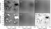 |
Fig. 2 A depiction of the cirrus subtraction method for the first iteration. Panel a) is the original SPIRE 500 μm image (all images on the same linear reverse grayscale, from −10 to 900 MJy/sr). Panel b) is the smoothed SPIRE 500 μm image that is used to fit the Gaussian shown in panel c). Panel c) is then subtracted from panel a) to produce a contrast image. A 4.25σ cutoff is then applied to the contrast image to produce the source masks shown in panel d). Panel d) is the original SPIRE 500 μm image with the sources masked out in white. This is the first iteration source masks; the final source boundaries are shown as white contours. Panel d) is then convolved with a Gaussian with the masks treated as missing data to produce panel e). Panel e) is considered the cirrus image for the next iteration. In the next iteration, a Gaussian will be fit to the cirrus image e), as a function of latitude at each longitude, and steps b)–e) will repeat. Panel f) is the difference image (original SPIRE 500 μm image a) – convolved cirrus image e)) that will eventually be used for greybody fitting in the final iteration. |
The first method for determining the dense clump source masks was to use Bolocat clump masks derived from the BGPS (Aguirre et al. 2011; Rosolowsky et al. 2010) at 1.1 mm. While these masks are a robust tracer of the cold, dense gas, they only extend to |b| ≤ 0.5° in the majority of our science field and the sensitivity in the ℓ = 59° field is too poor to trace the clumps seen in Hi-GAL.
The following methods all use the SPIRE 500 μm data to determine the source masks, as the cirrus decreases towards longer wavelengths (Gautier et al. 1992) and Peretto et al. (2010) demonstrate that the SPIRE 500 μm data is well-suited for cirrus/dense source distinction. The second method we tried was based on that of Peretto et al. (2010), who found that toward IRDCs, the SPIRE 500 μm flux distribution showed a clear peak at low fluxes with a long tail toward higher fluxes. While this method works well when applied to a single IRDC, as it was used in Peretto et al. (2010), it is not robust enough to be used to create a full Galactic cirrus emission map from high (| b| ≳ 1°) to low (| b| = 0°) Galactic latitudes. We then tried a third method to create the dense source masks using a simple contrast map (contrast = data – background) of the SPIRE 500 μm data and applied a cutoff. This method improved over the previous, however, it suffered from large negative bowls, creating source masks that were much smaller than the physical source sizes. In the fourth method, we define the background first by a second-order polynomial plane fit (along Galactic latitude) to the smoothed 500 μm image. This plane fit to the Galactic cirrus was then subtracted from the original data and a cutoff was applied (determined by eye) to define the dense source masks. This was the first method to do a reasonable job of identifying sources in a range of Galactic latitudes. We found, however, that a polynomial plane was not a very good approximation to the shape of the Galactic cirrus emission, and that the fit was particularly poor at high Galactic latitudes (| b| ~ 0.8−1°).
3.1.2. Final adopted method for source identification and Cirrus removal
Figure 2 depicts the final method used to identify the dense sources and to separate those from the cirrus cloud emission. The first panel (a) shows the original SPIRE 500 μm image. The first step (shown in panel b) is to convolve the 500 μm image with a Gaussian that is large enough to smooth over the sources but small enough to capture variations in the cirrus emission. We decided through trial and error that a Gaussian with a FWHM of 12′ was a reasonable compromise. We then fit a Gaussian in latitude to each Galactic longitude, as shown in Fig. 3 and in panel (c) of Fig. 2. A Gaussian is a reasonable approximation for the variation in the Galactic cirrus across the Galactic plane and worked to identify sources at high and low Galactic latitudes equally well. We then subtract the Gaussian fit approximation of the Galactic cirrus from the original 500 μm data to achieve a “difference image”. This “difference image” is the first guess at the cirrus-subtracted source map.
We apply a cutoff to this first guess cirrus-subtracted source map, such that everything above the cutoff is considered “source”. We determine this cutoff by fitting a Gaussian to the histogram of pixel values (as shown in Fig. 4). The negative flux values in the distribution of this “difference image” are representative of the random fluctuations in the data, so we mirror the negative flux values about zero, fit a Gaussian to that distribution (representative of the noise in the map) and then apply a cutoff of 4.25σ to the “difference image”. We calculated this cutoff in quarter σ intervals from 3 to 6σ, a range over which it grows smoothly. The choice of 4.25σ was selected because that cutoff best represented the sources in both the ℓ = 30° and ℓ = 59° fields when inspected by eye. While the choice of cutoff is important in determining the final physical properties, there is nothing special about this cutoff; the properties vary smoothly above and below this value.
Once the source cutoff has been determined, the sources are masked out in the original 500 μm image (as shown in solid white in panel (d) of Fig. 2) and we convolve (with a Gaussian of FWHM 12′) the data outside the source masks, the cirrus emission, treating data in the source masks as missing. This creates a second guess at the cirrus emission, equivalent to panel (b). We then repeat the process of fitting a Gaussian in latitude to this image (as in panel (c)), determining a source cutoff by fitting a Gaussian to the mirrored negative flux distribution in the “difference image”, applying these masks (panel (d)), and convolving around the masks (panel (e)) to produce the next guess at the cirrus emission (panel (b)). We iterate on this process until the source masks converge. Figure 5 shows the convergence of the source cutoff in both fields. We chose iteration 16 as the final source mask cutoff as it was representative of the converged value around which the iterations varied, though the exact choice does not matter much, as the cutoff varies very little after iteration 10 in both fields. In panel (d) of Fig. 2 the white masks are the first iteration source masks and the white contour shows the final (16th) iteration source masks. Once the source masks are determined, they are applied to each wavelength image, and that image is convolved (with a Gaussian FWHM 12′ and the mask pixels ignored) to create the cirrus image at that wavelength. Subtracting the cirrus image at each wavelength from the original data produces the source images used in the modified blackbody fits, while the smooth cirrus images are used for the modified blackbody fits to the cirrus emission.
The top panel of Fig. 3 shows a slice of 500 μm data through Galactic latitude. The final convolved background (dashed black line) is representative of the low-lying emission across Galactic latitude, including its asymmetry about b = 0°. Notice in the bottom panel that the structure is flat across Galactic latitude and allows for the identification of the source near b = 1°, demonstrating the success of the cirrus removal and source identification. The adopted method was the only of the five attempted which succeeded in identifying this source. The other methods failed to remove the cirrus emission at this high Galactic latitude sufficiently to allow identification of this source. Figure 4 shows that as the iterations converge, we move flux from negative bowls back to sources as positive features and the mirrored negative distribution then more closely resembles a Gaussian (the black line is the final Gaussian fit to iteration 16).
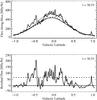 |
Fig. 3 A slice across the Galactic plane at ℓ = 30.51° of the SPIRE 500 μm image, demonstrating the cirrus emission removal method. The top panel shows the 500 μm data with the background fits (solid gray: first iteration Gaussian fit to the smoothed background, dashed gray: first iteration convolved background, solid black: same as gray, final iteration, dashed black: same as gray, final iteration). Note that the final background (dashed black line) fits the low-lying diffuse emission nicely, including its asymmetry about b = 0°. The bottom panel shows the final background subtracted science image cut along the same Galactic longitude, with the final source cutoff drawn as a dashed black line at 65 MJy/sr. |
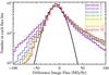 |
Fig. 4 The flux distribution in the difference images (original 500 μm image – convolved cirrus image, e.g. Fig. 2 panel f)) for 8 iterations from 1 to 20 in the ℓ = 30° field. In each iteration, the negative flux distribution was mirrored about 0 and a Gaussian was fit to the distribution to determine the characteristic fluctuations so that a source identification cutoff (of 4.25σ) could be applied. Plotted here are the full distributions, not the mirrored distributions used to fit the Gaussian. As we iterate, points in the negative end are transferred to the positive end of the distribution as flux is restored in the negative bowls around bright sources. The Gaussian fit to the distribution for the final iteration (16) is shown as the black curve. |
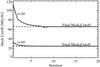 |
Fig. 5 The 4.25σ mask cutoff over 20 iterations. The cutoff is from the Gaussian fit (see Fig. 4) to the flux distribution of points in the difference image. Both the ℓ = 30° and ℓ = 59° fields converge after several iterations, but to very different values. |
This method has been fine-tuned by eye to reproduce the significant structure picked out by a human, but is entirely automated and was run in the exact same way for both the ℓ = 30° and ℓ = 59° fields, despite their vast differences. We have found that this method faithfully identifies sources across the range of Galactic latitudes covered by the data and the range of source confusion and activity observed. The sensitivity of this method is dependent upon the final mask cutoff or confusion, rather than the sensitivity of Hi-GAL. For the ℓ = 30° final mask cutoff of 65 MJy/sr, we are sensitive above the cirrus background to a column density of N(H2) = 2.9 × 1021 cm-2 for 20 K dust or N(H2) = 9.7 × 1020 cm-2 for 40 K dust. In the ℓ = 59° field the final mask cutoff is about 24 MJy/sr, which gives a sensitivity above the cirrus background to a column density of N(H2) = 1.1 × 1021 cm-2 for 20 K dust or N(H2) = 3.6 × 1020 cm-2 for 40 K dust.
3.2. Modified blackbody fits
We performed pixel-by-pixel modified blackbody fits to both the cirrus cloud and the dense source clump emission. The cirrus emission fits were performed on the 36′′ resolution images with all five Hi-GAL data points. β was allowed to vary as a free parameter. The dense source pixel-by-pixel fits were first performed on the images convolved to 36′′ resolution. Following that, the results from the 36′′ resolution tests were used as input to pixel-by-pixel fits performed on the images convolved to 25′′ resolution. While the fits to the 25′′ resolution images formally utilize less data points, they allow us to correlate the physical properties with star formation tracers on a smaller scale. We exclude the 500 μm (36′′ resolution) for the higher-resolution fit. The 70 μm point is also excluded because the optically thin assumption may not be valid (see Sect. 3.2.2 for more details). With only three data points for the fit, we fix β to a value of 1.75 (see Sect. 4.1 for details on how the results change if we instead assume a β of 1.5 or 2).
We use the modified blackbody expression in the form 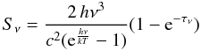 (1)where
 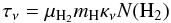 (2)where μH2 is the mean molecular weight for which we adopt a value of μH2 = 2.8 (Kauffmann et al. 2008), mH is the mass of hydrogen, N(H2) is the column density, and κν is the dust opacity. We determine the dust opacity as a continuous function of frequency by fitting a power-law of the form
  to the tabulated Ossenkopf & Henning (1994) dust opacities in the relevant range of frequencies. We used the Ossenkopf & Henning (1994) MRN distribution with thin ice mantles that have coagulated at 106 cm-3 for 105 years model for dust opacity, which is a reasonable guess for these cold, dense clumps. We have assumed a gas to dust ratio of 100, which yielded a κ0 of 4.0 at ν0 of 505 GHz with a β = 1.75.
3.2.1. Cirrus emission modified blackbody fits
We first fit a modified blackbody to each pixel in the cirrus image (e.g., Fig. 2 panel (e)) using MPFITFUN (from the Markwardt IDL Libarary, Markwardt 2009). We assign a calibration uncertainty of 20% to the SPIRE and PACS data points and use the covariance matrix returned by MPFITFUN to estimate errors in the parameters. In the modified blackbody fit, we leave the column density, β, and the temperature as free parameters. The temperature was restricted to range between 0 and 100 K, the column density was free to range between 0 and 100 × 1022 cm-2, and β from 1 to 3. We do not use the BGPS 1.1 mm point in the fits because uncertainties in both the absolute calibration and the spatial filter function prevent the BGPS point from significantly helping to constrain the fit at this time.
3.2.2. Dense source clump modified blackbody fits
We then fit a modified blackbody at each position within the source masks of the cirrus-subtracted science images (e.g., Fig. 2 panel (f)) to the dense clumps. For these fits of dense clumps, we ignore the 70 μm point since the optically thin assumption may not be valid (τ70 μm = 1 at N(H2) = 1.2 × 1023 cm-2 using Eq. (2)). In fact, IRDCs often appear in absorption at 70 μm indicating that in these very high column density regimes, the 70 μm data is not optically thin and that it can no longer be modelled by a single dust temperature. Additionally, it has been found (e.g., Desert et al. 1990; Compiègne et al. 2010) that a large fraction of the flux at 70 μm is likely contaminated by emission from very small grains whose temperature fluctuations with time are not representative of the equilibrium temperature of the large grains. Without the 70 μm point we have only four points (usually just on the Rayleigh-Jeans slope) to constrain the fit, so we fix β to 1.75 (Ossenkopf & Henning 1994), and leave only the temperature and the column density as free parameters. We discuss how a value of β of 1.5 or 2 would alter the results in Sect. 4.1. We acknowledge that perceived changes in temperature may actually be changes in β and discuss this more also in Sect. 4.1. We are, to an extent, looking for changes in the dust properties (β or temperature) across different environments, which we can still achieve.
These pixel-by-pixel modified blackbody fits to the cirrus-subtracted dense clumps were first performed on the images convolved to 36′′ resolution. Following that, the results from the 36′′ resolution tests were used as input to pixel-by-pixel fits performed on the images convolved to 25′′ resolution. While the fits to the 25′′ resolution images formally utilize less data points (the SPIRE 500 μm point must be excluded because of resolution), they allow us to correlate the physical properties with star formation tracers on a smaller scale. The physical properties returned by the fits at different resolutions agree well. The final temperature and column density maps (as shown in Fig. 6) show the derived temperatures and column densities from the 25′′ map within the source masks, and the smoothed cirrus-background temperatures and column densities outside the source masks.
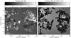 |
Fig. 6 Temperature (left) and Column Density (right) maps in the ℓ = 30° field test region. In these maps, the background cirrus emission temperature and column densities are plotted outside of the source masks, while the background-subtracted temperature and column densities are plotted inside the source masks. These maps are at 25′′ resolution and assume β = 1.75 inside the source masks. |
We note here that star-forming regions contain structure on many scales, and that fitting a single temperature and column density over a region of 25′′ (about 0.5 pc at a distance of 4 kpc) is a vast oversimplification. There certainly exist large variations in the temperature and column density in these sources on smaller scales. In this paper, we present the beam-diluted average source properties on 25′′ scales. The column densities presented here are therefore characteristic of the larger-scale clump structure and under-estimates of the peak column densities, while the temperatures will be underestimates in very hot regions (hot cores) and overestimates in very cold regions (starless IRDC cores).
3.3. Star formation tracer label maps
In order to robustly compare the physical properties determined in this paper with various star formation tracers, we have created star formation tracer label maps. These maps are on the same grid as the science images (temperature, column density, etc.) and have a binary denotion in each pixel: 1 if the star formation tracer is present and 0 if it is not. We create star formation tracer label maps for the MIPS 24 μm emission, 8 μm emission, EGOs (Cyganowski et al. 2008; Chambers et al. 2009), and 6.7 GHz methanol maser emission (Pestalozzi et al. 2005). The MIPS 24 μm images required stitching together using MONTAGE before the label map could be created. Since the ℓ = 30° field is more populated, we expect a wider range of star formation activity. This is, of course, assuming that the phase of star formation is generally random with location and that more regions will show a wider age distribution. For this reason, we choose to only perform the star formation tracer analysis on the ℓ = 30° field. The 8 μm emission label maps, however, were created and analyzed for both the ℓ = 30° and ℓ = 59° fields so that we could understand the relationship between mid-IR and Hi-GAL sources in both fields (see Sect. 4.4).
3.3.1. GLIMPSE 8 μm emission/absorption label map
The GLIMPSE 8 μm band shows emission from warm dust and polycyclic aromatic hydrocarbons (PAHs). Regions with bright 8 μm emission may contain warm, diffuse dust or UV-excited PAH emission from an Ultra-Compact HII Region (Battersby et al. 2010). The absorption of 8 μm emission by an IRDC is indicative of a high column of cold dust obscuring the bright mid-IR background. We note that mid-IR-bright regions are generally indicative of active star formation, and that the peak of mid-IR light can be offset from the youngest regions of star formation (e.g., Beuther et al. 2007). We denote regions of bright 8 μm emission as mid-IR-bright (mIRb), dark regions of absorption at 8 μm as mid-IR-dark (mIRd), and regions without stark emission or absorption at 8 μm as mid-IR-neutral (mIRn). The 8 μm emission label map has both a negative (IRDC, mIRd), positive (mIRb), and neutral (mIRn) component. This map is created by first making a contrast image. The GLIMPSE 8 μm image is convolved with a Gaussian of FWHM 5′ to represent the smooth, slowly varying background. 5′ was determined (see Peretto & Fuller 2009, for more details on this smoothing kernel choice) to be large enough to capture the largest IRDCs and mid-IR-bright objects, while still small enough to capture the background variations. This image is then subtracted from the original image, which is then divided by the smoothed background. The resulting “contrast map” enhances the contrast of mIRb and mIRd clouds above the bright mid-IR background. To obtain a fair comparison with the lower resolution (~25′′) science images, this contrast image is convolved to the same resolution. We then apply a cutoff such that any pixel with a positive contrast greater than or equal to 10% is considered mIRb, and any pixel with a negative contrast greater than or equal to 5% is considered mIRd, while all others are then mIRn. We rely on our eyes to pick out regions of emission and absorption, and have selected the cutoffs that best represent a visual interpretation of that which is dark and bright, as shown in Fig. 7.
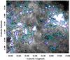 |
Fig. 7 GLIMPSE 8 μm image overlaid with contours of the classification as mid-IR-bright (mIRb, dark blue) or mid-IR-dark (mIRd, cyan). The classification is only applied where a far-IR source exists, as denoted by the black contours. |
A portion of this label map is shown in Fig. 7. This method does a very good job of picking out the bright and dark regions, and agrees reasonably well (considering the different methods, resolution used, and cutoffs) with the IRDC catalog of Peretto & Fuller (2009). Two important biases to note with this method are: 1) the contrast image technique creates “negative bowls” around bright objects, and therefore the sizes of the mIRd and mIRb regions are underestimated, and 2) convolving the contrast image to 25′′ resolution causes us to miss some small IRDCs. Additionally, any decrements in the background will be denoted as being mIRd. This issue is partly resolved when we multiply this label map with our source masks, so that our classifications only apply where a Hi-GAL source also exists.
3.3.2. MIPSGAL 24 μm emission label map
Emission at 24 μm observed using the MIPS instrument traces warm dust. MIPS 24 μm emission can trace warm, diffuse dust in the ISM or warm dust associated with star formation such as material accreting onto forming stars, the gravitational contraction of a young stellar object, or warm dust surrounding a newly formed star. The MIPS 24 μm emission label map was created using the same method as the 8 μm label maps, with the exception that we only include a positive contrast cutoff. While some IRDCs remain dark at 24 μm, the negative contrast is very minimal when convolved to 25′′ resolution. Additionally, the highest negative contrast in the contrast image is from the negative bowls around bright sources, so identifying IRDCs in the 24 μm images using this method is not adequate. The positive contrast threshhold for the MIPS 24 μm contrast maps was 25%, also chosen by eye. A higher cutoff than at 8 μm was required to select the 24 μm sources above the bright background. These cutoffs greatly affect the resulting trends. See Sect. 4.1 for a discussion of the effects of cutoffs on source identification.
3.3.3. Extended green objects label map
We include the presence of EGOs (also called “green fuzzies” Cyganowski et al. 2008; Chambers et al. 2009) as a star formation tracer. EGOs are regions of enhanced and extended 4.5 μm emission and are thought to be indicative of shocks in outflows (Cyganowski et al. 2009). Cyganowski et al. (2008) catalogued EGOs throughout the Galaxy in the GLIMPSE fields. There are two “possible” EGOs in the ℓ = 30° field which we include in our EGO label map. We supplemented the Cyganowski et al. (2008) catalog with an independent visual search of the ℓ = 30° field for EGOs that may have been missed. An independent, cross-checked search identified eight further candidates, which we include in our analysis. A list of the locations of the EGOs used in this analysis is given in Table 1, and they are shown in Fig. 8. For each EGO, a box was drawn around the region that contains the EGO, and each pixel in this box was given a flag of 1, while for pixels outside the box the flag is 0.
EGOs used in this paper.
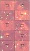 |
Fig. 8 GLIMPSE 3-color images (red: 8 μm, green: 4.5 μm, blue: 3.6 μm) of EGOs in the ℓ = 30° field. The EGOs shown in the right column of the 3rd and 4th row were identified as “possible” EGOs by Cyganowski et al. (2008) and the others were identified by two independent viewers as EGOs as described in Sect. 3.3. The positions are listed in Table 1. |
3.3.4. 6.7 GHz Class II CH3OH masers label map
Finally, we employ the presence or absence of 6.7 GHz Class II CH3OH masers as a star formation tracer. We use the complete catalog compiled by Pestalozzi et al. (2005) to identify unbiased searches for 6.7 GHz methanol masers in the ℓ = 30° field. While there have been numerous targeted searches for CH3OH masers, we utilize the unbiased Galactic plane searches of Szymczak et al. (2002) and Ellingsen et al. (1996), on the 32 m Torun Radio Telescope (FWHM of 5.5′) and the University of Tasmania 26 m Radio Telescope (FWHM of 7′), respectively. 6.7 GHz methanol masers are found to be exclusively associated with massive star formation (Minier et al. 2003), and are often offset from the radio continuum emission indicative of an UCHII Region (e.g., Walsh et al. 1998; Minier et al. 2001) and are thought to represent an earlier stage of massive star formation. We chose to include only the unbiased catalogs of Ellingsen et al. (1996) and Szymczak et al. (2002) so as not to choose mIRb regions preferentially. These catalogs together give 22 methanol maser regions, which we use to create a label map where the “size” of the methanol maser regions is given by 2 × the positional accuracy rms of the observations (30′′ and 36′′ for Szymczak et al. 2002; Ellingsen et al. 1996, respectively). Methanol maser emission comes from very small areas on the sky (e.g., Walsh et al. 1998; Minier et al. 2001), however, methanol masers are often clustered (Szymczak et al. 2002; Ellingsen 1996, find multiple maser spots towards the majority of sources), so these “source label sizes” are meant to be representative of the extent of the star-forming region.
4. Results
We discuss here the results of the modified blackbody fits, the properties of the Galactic cirrus emission, a comparison of mIRb and mIRd pixels, and the association with star formation tracers. We discuss what defines the populations of mIRb and mIRd sources, and the objects which have no mid-IR association. Before the discussion of the results, we first mention the many caveats and uncertainties that accompany these findings.
4.1. A remark on caveats and uncertainties
A major uncertainty in this analysis is the modified blackbody fits. Firstly, star-forming regions show structure on many scales, and so fitting a single column density and temperature to any point does not adequately represent the whole region; rather it serves as a way to categorize and differentiate between bulk, large-scale physical properties of regions. Additionally, this means that the quantities derived are likely to be highly beam-diluted. The true peak column density in any given region is almost certainly higher than the beam-averaged column density reported here. Likewise, the beam-averaged temperatures reported for cold objects are overestimates of the true temperature minimum, while the beam-averaged temperatures reported for hot objects is an under-estimate of the peak. These caveats explain the somewhat small dynamic range observed in both temperature and column density.
In addition, the parameters derived from the modified blackbody fits themselves are rather uncertain. For most of the sources, the temperature is higher than 18 K, so all the points used in the fit lie near the peak of the SED or on the Rayleigh-Jeans slope. This equates to large uncertainties in the fits, especially at high temperatures. The median errors in the derived temperature are about 4 and 3 K (for the ℓ = 30° and ℓ = 59° fields, respectively), while the median errors in the derived column density are about 0.12 and 0.04 × 1022 cm-2 (in ℓ = 30° and ℓ = 59° fields, respectively). The error is a strong function of the parameter value, with a median temperature error of 13% and 18% and median column density error of 44% and 48% (in the ℓ = 59° and ℓ = 30° field, respectively). These uncertainties are based on the 20% calibration uncertainty assigned to the Hi-GAL fluxes. Additionally, the derived quantities are highly dependent not only on the background that is subtracted, but also on possible departures between the gain scale of the PACS and the SPIRE data. Improvements to the general issue of the Planck-Herschel cross calibration with respect to the accuracy of the offset determination as well as to the gain values will be adressed in the future.
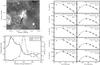 |
Fig. 9 Top left: GLIMPSE 8 μm image in our ℓ = 30° test region. Right: modified blackbody fits to the points marked on the filament in the top left panel. Since the 70 μm point is not included in these fits (see Sect. 3.2) it is plotted as an X while the other points are shown with their 20% calibration error bars. The errors quoted in temperature and column density are the formal fit errors. As discussed in Sect. 4.1, these are not necessarily representative of the true errors. Bottom left: the temperature and column densities derived along the filament, with 10 points marked. Note the inverse relation between temperature and column density in this example, especially from points 8 to 10. |
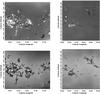 |
Fig. 10 Top: temperature (on a linear scale from 0 to 50 K) and bottom: column density (on a log scale from N(H2) = 0 to 5 × 1022 cm-2) in the ℓ = 30° (left) and ℓ = 59° (right) fields. In these maps, the background cirrus emission temperature and column densities are plotted outside of the source masks, while the background-subtracted temperature and column densities are plotted inside the source masks. These maps are at 25′′ resolution and assume β = 1.75 inside the source masks. |
The assumption of a fixed β can be considered to contribute the bulk of the uncertainty in the temperature determination. The degeneracy of β-T has been discussed in Paradis et al. (2010). If we adopt a value of β = 1.5 (instead of 1.75), the temperatures are about 4 K higher on average and the column densities are about the same. If we adopt a value of β = 2.0 (instead of 1.75), the temperatures are about 3 K lower on average, and again, the column densities are about the same. With only four data points to constrain the fits, fixing β is nearly essential, with the choice of 1.75 being a reasonable guess for these environments. Variations in β from 1.75 to 1.5 or 2 correspond to changes in temperature of about 3 or 4 K. There is the possibility that systematic changes in β, for example a systematic decrease in β toward the center of IRDCs due to dust coagulation (Ossenkopf & Henning 1994), could systematically change our results. In the dark centers of IRDCs, however, a variation in β only changes the temperature by about 2 K (2 K hotter for β = 1.5, and 2 K colder for β = 2.0), so while this is an important effect to consider, it is unlikely to negate the observed trends in temperature.
The association with star formation tracers is also bridled with uncertainty. Each of the tracers included are not perfectly represented with our methods. The 8 and 24 μm label maps are entirely dependent on the cutoffs chosen. While we have done our best to choose reasonable cutoffs, a change in these cutoffs would have a significant effect on the properties inferred. The association with EGOs suffers from a similar bias. We have made a careful attempt to identify probable EGO candidates, but the objects themselves are somewhat ill-defined, so again, we resort to the by-eye classification. The association with CH3OH masers is robust in that it is based on uniform sensitivity blind surveys, however, these surveys suffer from large beam sizes and confusion which consequently dilute their true physical properties. All of these tracers also suffer from the inherent scatter that comes along with varying levels of extinction and different distances.
Despite these caveats, the trends observed over many pixels remain robust. The pixel-by-pixel comparison is an important technique for achieving the best possible associations with the given data, and therefore, the most robust statistics. The object in the center of Fig. 9 highlights the importance of comparing values on a pixel-by-pixel basis, rather than denoting the entire object as either mIRb or mIRd.
4.2. Properties of the Cirrus cloud emission
The diffuse Galactic cirrus emission, identified early with IRAS (Low et al. 1984), is thought to be due to the ISM, which is constantly being injected with energy through spiral shocks and stellar feedback. The emission we see as cirrus most likely comes from a large column of diffuse dust, rather than a single cloud. Various studies have characterized the cirrus noise through its power spectrum (e.g., Gautier et al. 1992; Miville-Deschênes et al. 2007; Roy et al. 2010) and most recently, Martin et al. (2010) have performed a direct estimate of cirrus noise using Hi-GAL.
While we primarily consider the cirrus cloud emission as “background” in this paper, we report here some useful physical properties derived in this analysis. These maps were smoothed to 12′ (ΘFWHM) resolution, so we report only the average properties in Table 2. These data suggest that dust in diffuse clouds in the molecular ring (ℓ = 30° field) is warmer, has higher column densities, and a steeper spectral index (β) than dust in diffuse clouds toward the mid-outer Galaxy, outside the molecular ring (ℓ = 59° field). In the cirrus background determination, we fit a Gaussian of the form: g = B + Ae(b − b0)2/2σ2 across Galactic latitude at each Galactic longitude. We report here the Gaussian fit to the median value across Galactic longitudes. In the ℓ = 30° field, the best fit parameters are A = 285 MJy/sr, B = 38 MJy/sr, b0 = −0.1°, and σ = 0.4°, while in the ℓ = 59° field, the best fit parameters are A = 53 MJy/sr, B = 29 MJy/sr, b0 = 0.1°, and σ = 0.4°. Previous studies (e.g., Rosolowsky et al. 2010) have shown that the mean Galactic latitude where emission peaks depends strongly on the Galactic latitude observed, but that the mean in the First Galactic Quadrant is ⟨ b ⟩ ≈ −0.1°. This negative value of the mean Galactic latitude may be related to the location of the sun in the Galaxy. The ℓ = 30° field also shows an average Galactic latitude of about −0.1°, while the ℓ = 59° field is higher than the average at b0 = 0.1°. It should be noted that the value of mean Galactic latitude of emission can be severely biased due to the presence of large cloud complexes, especially in small fields.
Smoothed cirrus emission properties.
4.3. The temperature and column density maps
We present full temperature and column density maps of the Hi-GAL ℓ = 30° and ℓ = 59° SDP fields. These maps are shown in Fig. 10 and will be available for download as FITS files online with the Hi-GAL data when the processed data is released publicly. The source mask label maps, the source mask temperature and column density maps, the error maps of these quantities, the cirrus emission temperature, column density, and β maps, and their error maps as well as the star formation tracer label maps will all be available for download. The maps presented in Fig. 10 are displayed such that the values inside the source masks represent the background-subtracted fit values, while the values outside the source mask are the fits to the background itself.
The uncertainties in these maps are discussed in Sect. 4.1. In addition to those, we found that in the ℓ = 30° field, our fits were returning unsensible parameters at high Galactic latitudes (| b| ≳ 0.8°). This is due to imperfect calibration of the zero-level offsets which is especially problematic at high Galactic latitudes where the flux levels are already low. This imperfect calibration negates any physical meaning in the relative fluxes of the Hi-GAL bands in this region. We do not see this same problem in the l = 59° field, presumably due to the overall lower variance in flux values from high to low Galactic latitudes. We made several attempts at correcting or properly ignoring those points, with little success, and therefore, recommend that the maps in the ℓ = 30° field only be used within |b| ≤ 0.8°. Additionally, pixels near the edges of the source masks were just barely above the background, and can produce unphysical fits, so be cautious of any pixel that is right on the edge of the source mask.
The column density follows the far-IR flux closely, while the temperature is quite varied, and in many cases, inversely correlated with the column density. The median temperatures for all the pixels in the source masks are 26 and 20 K, while the median column densities are 0.25 and 0.10 × 1022 cm-2 (for the ℓ = 30° and ℓ = 59° field, respectively). The highest column density points are found in W43, the large complex near ℓ = 30.75°, b = −0.05° (Bally et al. 2010), where the bright millimeter points, MM1−MM4, have beam-averaged column densities of around 1023 cm-2.
4.4. The association of Far-IR clumps with mIRb and mIRd sources
The association of Hi-GAL sources identified in the Far-IR with mid-IR sources is of interest, as that gives some indication of their star-forming activity. We find that Hi-GAL sources span the range of pre- to star-forming and that there exist significant trends in both temperature and column density between these populations. The growing interest in IRDCs as potential precursors to stellar clusters emphasizes the importance of identifying IRDC-like sources throughout the Galaxy in an unbiased manner, not just where they exist in front of a bright mid-IR background. A survey such as Hi-GAL is essential to identify IRDC-like objects throughout the Galaxy while a thorough analysis is necessary for understanding the trends in Hi-GAL sources that are pre- versus star-forming.
We find that mIRd pixels are characterized by colder temperatures (colder by more than 10 K) and higher column densities (about a factor of two higher) than mIRb pixels (see Table 3). The mIRn pixels generally have a column density similar to that of mIRb pixels, and a temperature midway between mIRd and mIRn pixels (see Fig. 11). This trend is also apparent in the left panel of Fig. 12. The mIRn points at the extreme left in the left panel of Fig. 12 are due to the imperfect definition of the 8 μm masks. Where mIRb and mIRd regions are adjacent, the pixels between are denoted as mIRn since the two adjacent regions are blurred. This causes some pixels to be denoted as mIRn which may truly be mIRd or mIRb. Figure 11 shows that introducing a column density cutoff to the temperature distribution decreases the average temperature, especially for mIRb pixels. If, on the other hand, we introduce a temperature cutoff (T < 25 K) to the column density distributions, the average column density increases.
Source properties by their mid-IR association.
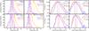 |
Fig. 11 Normalized temperature and column density histograms of source pixels in the Hi-GAL fields separated by their 8 μm association; mid-IR-dark (mIRd), mid-IR-neutral (mIRn), or mid-IR-bright (mIRb). The values printed on the plots are the medians of the distributions (also seen in Table 3). The mIRd pixels tend to have the lowest temperature and highest column density, while the mIRb pixels have the highest temperature and lowest column density, and the mIRn pixels fall in the middle. Left: normalized temperature histograms in the ℓ = 30° (left) and ℓ = 59° fields (right), top panels include all source pixels while the bottom panels only include source pixels above a column density cutoff. Introducing this column density cutoff decreases the average temperature, especially for the mIRb pixels. Right: normalized percentage logarithmic column density histograms in the ℓ = 30° (left) and ℓ = 59° fields (right), top panels include all source pixels while the bottom panels only include source pixels with a temperature below 25 K. These low temperature pixels have higher column densities on average, especially the mIRb ones. |
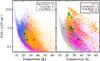 |
Fig. 12 Left: a column density versus temperature plot comparing mIRn (8 μm neutral, magenta), mIRd (8 μm dark, blue), and mIRb (8 μm bright, orange) pixels within the ℓ = 30° source masks, with the median of each value plotted as a diamond on top. The mIRd points occupy the coldest, highest column density portion of the plot, while the mIRb points occupy a range of column densities and warmer temperatures. The mIRn points at the extreme left of the plot are due to the imperfect definition of the 8 μm masks. Right: a similar plot as the left, but with all points (gray), points associated with a CH3OH maser (orange) or EGO (green), and 24 μm bright points (magenta). We note that EGOs occupy a mid-range temperature and the highest column density portion of this plot, while the CH3OH maser points occupy a wide mid-range of temperatures and a high range of column densities. The 24 μm points are associated with higher temperature points and relatively low column density. |
A simple K-S test rules out the possibility that any combination of the mIRd, mIRn, or mIRb populations in temperature or column density are drawn from the same distribution with at least 99.7% confidence. For the K-S test, we calculated the effective number of independent points in each distribution by dividing the number of pixels in each distribution by the number of pixels per beam. Considering the errors discussed in Sect. 4.1, these trends are significant and not likely to be a by-product of systematic errors. Hi-GAL is sensitive to both cold, high column density, likely pre-stellar sources and warmer, more diffuse star-forming regions. We can distinguish between these using the temperature and column densities derived simply from Hi-GAL or through comparison with other tracers.
In Fig. 13, we plot the fraction of mIRd, mIRn, and mIRb pixels above the column density cutoff plotted on the x-axis. In the ℓ = 30° field, the mIRn fraction drops quickly as the mIRd fraction rises, while in the ℓ = 59° field, mIRb fraction rises steadily as the mIRn fraction drops. While assigning an overall percentage to each of the categories is somewhat subjective, because of the cutoff-dependent variations, we estimate that in the ℓ = 30° field about 55% of the Hi-GAL identified source pixels are mIRd, 20% are mIRn, and 25% are mIRb. In the ℓ = 59° field, we estimate that about 20% of the Hi-GAL identified source pixels are mIRd, 40% are mIRn, and 40% are mIRb. The fact that the fraction of mIRd pixels in the ℓ = 59° field is so much lower than that in the ℓ = 30° field could be an artifact of the relatively sparse mid-IR background emission in the ℓ = 59° field, or it could very well be that there is a lower fraction of cold, high-column density clouds in the ℓ = 59° field.
4.5. Star formation tracers in Hi-GAL sources
We compare the temperature and column density maps with the star formation tracer label maps (discussed in Sect. 3.3). While we evaluate the evolution of sources by their temperature alone, Beuther et al. (2010) analyze the evolution of four sources with changes over the entire SED. We find that the more star formation tracers associated with a source, the higher the temperature (see Fig. 14 right). This trend is not surprising: a star-forming clump will be warmer than a pre-star-forming clump. It is reasonable to assume that as a clump evolves, the temperature will increase monotonically. Therefore, we compare the individual star formation tracers with temperature to see if there is any indication about which star formation tracer may turn on first, and what the relative lifetimes might be. There are a lot of uncertainties in this analysis (discussed in 4.1) and we are comparing beam-averaged physical parameters, so there is quite a lot of scatter.
In the left panel of Fig. 14 we see a progression of star formation tracers with temperature, with a huge amount of overlap. The median temperatures of each population (denoted with a dotted line, and stated in the legend) delineate a sequence from cold pre-stellar clumps to warm star-forming clumps, from mIRd, to outflow/maser sources, to sources which are bright at 8 and 24 μm. However, the overall distributions are very wide, possibly indicating long lifetimes, but more likely an indication of large errors in both the beam-averaged physical properties and the assignment of star formation tracers.
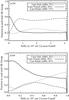 |
Fig. 13 Fraction of pixels in each mid-IR categorization (mIRd, mIRn, mIRb) as a function of column density cutoff for the ℓ = 30° (top) and ℓ = 59° (bottom) fields. In the ℓ = 30° field, as the column density cutoff is increased, the mIRd pixels become much more prevalent, replacing the common, but low-significance mIRn pixels, whereas in the ℓ = 59° field, the mIRb pixels become more prevalanet as the mIRn contribution lowers. We conclude that in the ℓ = 30° field, about 55% of the far-IR sources are mIRd, 20% are mIRn, and 25% are mIRb, while in the ℓ = 59° field, about 20% are mIRd, 40% are mIRn, and 40% are mIRb. It is evident from these plots, however, that these numbers are somewhat subjective and can vary depending on the cutoff selected. |
Figure 12 shows these trends in both temperature and column density space. The left panel shows that mIRd pixels are generally colder and have higher column densities than mIRb pixels. The right panel shows that all the star formation tracer pixels are warmer than the mIRd population, with CH3OH masers in the mid-range of temperatures, and 24 and 8 μm bright pixels occupying the highest temperature range. EGOs are characterized by a similar temperature as CH3OH masers, but a slightly higher column density. Interestingly, the EGOs seem to occupy two distinct regions on the plot in Fig. 12, one higher and one lower column density, indicating that EGOs are present in a variety of environments. It is not surprising that the EGOs represent the highest column density population, as they are the most localized star formation tracer we have used.
We perform simple K-S tests to determine the likelihood that any combination of the temperature or column density distributions of star formation tracers (pixels which are mIRd, mIRb, 24 μm bright, or contain EGOs or masers) are drawn from the same distribution. For the K-S test, we calculated the effective number of independent points in each distribution by dividing the number of pixels in each distribution by the number of pixels per beam (about 23 in the 25′′ resolution images used for all tracers except the masers, which have an accuracy of about 33′′, or 41 pixels). Since EGOs are defined locally, each pixel is considered independent. When we compare the temperature distributions of all combinations of the mIRd, mIRb, 24 μm bright, EGO and maser populations, we can rule out with at least 99.7% confidence that any are drawn from the same distribution, except the 24 and 8 μm bright points, which have about a 55% probability of being drawn from the same distribution, and the EGO and maser populations which have about a 0.5% chance of being drawn from the same distribution. When we compare the column density distributions of all combinations of the mIRd, mIRb, 24 μm bright, EGO and maser populations, we can rule at with at least 99.7% confidence that any are drawn from the same distribution, except the EGO and maser populations, which have about a 55% chance of being drawn from the same distribution. The fact that EGOs and CH3OH masers may be tracing the same population of sources is encouraging, as they are both supposed to trace young, massive outflows. We would also have expected that pixels which are bright at 8 or 24 μm should be tracing similar environments, as both can be excited by the heat or UV light from a young, accreting protostar.
We see interesting trends in Hi-GAL clumps between temperature and column density and star formation tracers. We find that 8 μm dark pixels are, on average, the coldest, followed by pixels containting EGOs and/or CH3OH masers, then 8 and 24 μm bright points. If we assume that as a clump evolves, it will monotonically increase in temperature with time, then this could suggest a possible sequence of tracers. However, the scatter is still too large to suggest a definitive sequence or lifetimes. We should expect that one of the first stages will be the formation of an outflow, detectable by an EGO or CH3OH maser. Following that, the protostar will continue to heat its surroundings and light up at 24 μm. A massive protostar may form an UCHII region while still accreting, whose UV light would excite PAHs in the 8 μm band of GLIMPSE. Unlike Battersby et al. (2010), we find that 24 μm sources light up around the same time as 8 μm sources. This is almost certainly due to the use of a high, automated cutoff to determine the existence or absence of a 24 μm source. In Battersby et al. (2010), UCHII regions were associated with very bright (≳ 1 Jy) 24 μm point sources, which may be the population of bright sources we are picking out here. We note that even though most or all UCHII regions are mIRb, certainly not all mIRb sources are UCHII regions (e.g., Mottram et al. 2010). The fact that the population of mIRb and 24 μm bright are so similar is likely an artifact of the cutoffs chosen. The two should be associated for bright sources, which is the trend we see in this paper, but for dimmer sources, which are excluded by the cutoff, we do not know the association. The detection of an EGO or 24 μm point source depends on the exinction and the background, and the sensitivity for detection will decrease with distance. As discussed, there are many caveats and systematic errors to consider, however, the trends are intriguing.
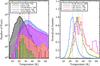 |
Fig. 14 A comparison of star formation tracers in the ℓ = 30° field. The identification of these tracers is discussed in Sect. 3.3. Left: Log histogram of the temperature distributions for all source pixels identified as mIRd (8 μm dark, black), associated with EGOs (green) or a CH3OH maser (orange), mIRb (8 μm bright, blue), or 24 μm bright (magenta). The median temperature is reported in the legend and with the dashed vertical line for each tracer. If one assumes that a source will monotonically increase in temperature with time, this diagram gives a possible indication of the observed evolution of sources in this field. Right: a normalized temperature histogram for all pixels in the ℓ = 30° source masks containing 0 (blue), 1 (green), 2 (orange), and 3 (magenta) of the star formation tracers shown in the left panel. The pixels containing 4 star formation tracers are rare, follow the distribution of the EGOs, and have low number statistics and therefore are not plotted. The median temperature is again reported in the legend and with dotted vertical lines. This plot shows that warmer pixels are associated with more star formation tracers. |
Far-side IRDC candidates.
5. IRDC-like source candidates on the far-side of the Galaxy
We present a list of candidate IRDCs on the far-side of the Galaxy in Table 4. These sources are cold (~20 K), high column density (>1 × 1022 cm-2) objects identified in Hi-GAL with very weak absorption at 8 μm. These are objects that, were they in front of the bright mid-IR background, should be IRDCs, but are not. To identify these sources, we calculated an extinction column density map at 8 μm, using the method of Peretto & Fuller (2009) and compared this with the Hi-GAL column density map. Any sources with a Hi-GAL column density >1 × 1022 cm-2 and an extinction column density several (3−4) factors lower was considered. We performed an examination by eye simply to check that these are plausible candidates. The extinction must be weak, the region cannot be mIRb, and it needs to be cold (<30 K). In other words, these are sources that, if on the near-side of the Galaxy, should be dark at 8 μm, yet they are not. None of these sources are identified as IRDCs by the catalog of Peretto & Fuller (2009). Sources at high Galactic latitudes (| b| ≳ 0.5°) and in the ℓ = 59° field were not included because the sparse background adds additional uncertainty to the extinction column density estimate.
We discuss G030.01-0.27, a candidate far-side IRDC, in more detail here as an example of this class of objects. G030.01-0.27 is a high-column density (~3 × 1022 cm-2), cold (~20 K) dust continuum source in the ℓ = 30° field near the Galactic mid-plane that is not 8 μm dark (see Fig. 15). There is a slight decrement at 8 μm that is nearly consistent with background fluctuations as this source was not detected in the IRDC catalogs of Peretto & Fuller (2009) or Simon et al. (2006). At 70 μm, this source breaks up into two, a Southern source at (ℓ, b) = (30.009, −0.274) and Northern source at (ℓ, b) = (30.003, −0.266). The Southern source appears to be very small and faint at 8 μm, while the Northern source is a faint, slightly extended source at 8 μm. The Southern source has bright 24 and 70 μm emission. The Northern source is also seen in emission at these wavelengths, though less brightly. Comparison with the MAGPIS (Helfand et al. 2006; White et al. 2005) 20 cm maps show no emission in the radio continuum coincident with either source, while the MAGPIS 6 cm map shows a very faint object associated with the Southern source. This emission (at 8 μm and the faint emission at 6 cm) is indicative of some star formation activity, while the cold dust temperature and high column density indicate cold, dense gas available for further star formation.
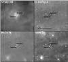 |
Fig. 15 A possible IRDC-like source on the far-side of the Galaxy. This source is cold (~20 K), has high column density (~3 × 1022 cm-2) and is amidst the bright mid-IR Galactic Plane at (ℓ, b) = (30.01, −0.27). By these measures, it should be an IRDC, but the 8 μm image (top right) shows only a moderate decrement and the near-side extinction column density is almost an order of magnitude less than expected from the far-IR column density. This source breaks up into a Northern (ℓ, b) = (30.003, −0.266) and Southern (ℓ, b) = (30.009, −0.274) component at the higher resolution of the PACS 70 μm band. This source is a great candidate for further study. |
The faint decrement at 8 μm can be morphologically matched with a molecular cloud in 13CO (Jackson et al. 2006, from the Galactic Ring Survey) at about 104 km s-1. Integrating from 100 to 108 km s-1, assuming 20 K, and using Eq. (17) from Battersby et al. (2010) the column density is about 2.5 × 1022 cm-2, consistent with the Hi-GAL column density estimate. Using the rotation curve of Reid et al. (2009), the near-side distance of this 13CO cloud is 5.8 kpc and the far-side distance is 8.7 kpc. Using the extinction mass determination technique of Butler & Tan (2009) as applied in Battersby et al. (2010), the 8 μm extinction column density of the cloud is 0.5 × 1022 cm-2 assuming it is on the near-side of the Galaxy or 1 × 1022 cm-2 assuming it is on the far-side of the Galaxy. It is not expected that the extinction column density estimation method will be very robust for clouds on the far-side of the Galaxy, but this very slight extinction is at least consistent with the cloud being on the far-side of the Galaxy. Additionally, this cloud shows no obvious HI self-absorption (Stil et al. 2006). While none of this evidence is conclusive, it all seems to indicate that this cloud is on the far-side of the Galaxy. Another possibility, however, would be that this cloud is simply behind the majority of the diffuse mid-IR emission, and still on the near-side of the Galaxy. Either way, it is an interesting source that was otherwise missed as such in previous study.
The fact that the mid-IR background is bright at the locations of these sources, yet the 8 μm extinction column density is extremely low is a strong indication that these sources are behind the bright mid-IR background. In fact, the Hi-GAL distance analysis by Russeil et al. (2011) finds that all the sources in Table 4 are either at the far or tangent distance (>7 kpc) except for G029.28-0.33, which is on the near-side at about 6 kpc, so still likely behind most of the bright mid-IR emission.
With their high far-IR column density and low temperature, these sources are easily categorized (based on the left panel of Fig. 12) as IRDC-like. These are the first candidate far-side IRDCs of which the authors are aware. The potential outer Galaxy IRDC identified by Frieswijk et al. (2007) is similar in that they are both IRDC-like objects identified independent of 8 μm absorption. However, these sources are not in the outer Galaxy, but on the far-side of the inner Galaxy. These candidates are just a few of potentially many more IRDC-like sources which remain to be uncovered in a study like this over the Galactic plane.
6. Conclusions
We have performed cirrus-subtracted pixel-by-pixel modified blackbody fits to the Hi-GAL ℓ = 30° and ℓ = 59° SDP fields. The source identification and cirrus-subtraction routines are robust and can be applied to Hi-GAL data throughout the Galactic plane. We present temperature and column density maps of the dense clumps in these fields and cirrus column density, temperature, and β maps. We find that the cirrus cloud emission is characterized by β = 1.7, N(H2) = 0.7 × 1022 cm-2, and T = 23 K in the ℓ = 30° field and β = 1.5, N(H2) = 0.3 × 1022 cm-2, and T = 21 K in the ℓ = 59° field.
We also characterize each pixel as mid-IR-bright (mIRb), mid-IR-dark (mIRd), or mid-IR-neutral (mIRn), based on the contrast at 8 μm. The association of Hi-GAL sources identified in the far-IR with mid-IR sources is of interest, as the far-IR sources span the range of pre- to star-forming regions, and the mid-IR can help to separate these. We find that in the ℓ = 30° field, about 55% of the pixels are mIRd, 20% are mIRn, and 25% are mIRb, while in the ℓ = 59° field, about 20% are mIRd, 40% are mIRn, and 40% are mIRb. There exist significant trends in temperature and column density between the populations of mIRd to mIRb. We find that mIRd dark pixels are about 10 K colder and a factor of two higher column density than mIRb pixels. The mIRd pixels are likely cold pre-star-forming regions, while the mIRb pixels are in regions that have probably begun to form stars. It is important to note that mIRd pixels may be forming low-mass stars which are simply embedded and not seen at these distances, and that these regions are not necessarily pre-cursors to massive star forming regions. This study has shown that Hi-GAL-identified sources span the range from cold, pre-star-forming to actively star-forming regions.
We also include the presence or absence of EGOs (indicative of shocks in outflows), CH3OH masers, and emission at 8 and 24 μm as star formation tracers. We find that warmer pixels are more often associated with star formation tracers and also that the warmer a pixel is the more star formation tracers it is associated with, as seen in Fig. 14. We also find a wide but plausible trend in temperature, where the coldest pixels, on average, are mid-IR-dark, followed by pixels containing EGOs and/or CH3OH masers, then 8 and 24 μm bright sources. While the systematic errors are too large to suggest an evolutionary sequence, this trend is intriguing.
Finally, we identify five candidate far-side IRDCs. These objects are cold (~20 K), high column density (>1 × 1022 cm-2) sources identified with Hi-GAL that have very weak or no absorption at 8 μm. We explore one such candidate in more detail in Sect. 5. This object at roughly (ℓ, b) = (30.01, −0.27) has a high far-IR column density (N(H2) ~ 3 × 1022 cm-2), is cold (~20 K) and in a position near an abundantly bright mid-IR background, yet shows almost no decrement at 8 μm. In fact, the 8 μm extintion-derived column density is almost an order of magnitude lower than expected from the far-IR estimate. These candidate far-side IRDCs are the first of their kind of which the authors are aware. This type of analysis will likely uncover many more such objects. With a complete sample of IRDC-like (cold, high column density) clouds, independent of the local mid-IR background, one could map the clouds in the earliest stages of star-formation over the entire Galaxy.
Acknowledgments
The authors are grateful to the anonymous referee whose insight has helped to improve the quality of this manuscript. Data processing and map production has been possible thanks to generous support from the Italian Space Agency via contract I/038/080/0. Data presented in this paper were also analyzed using The Herschel interactive processing environment (HIPE), a joint development by the Herschel Science Ground Segment Consortium, consisting of ESA, the NASA Herschel Science Center, and the HIFI, PACS, and SPIRE consortia. This research made use of Montage, funded by the National Aeronautics and Space Administration’s Earth Science Technology Office, Computation Technologies Project, under Cooperative Agreement Number NCC5-626 between NASA and the California Institute of Technology. Montage is maintained by the NASA/IPAC Infrared Science Archive. This work made use of ds9, the Goddard Space Flight Center’s IDL Astronomy Library, and the NASA Astrophysics Data System Bibliographic Services. C.B. is supported by the National Science Foundation (NSF) through the Graduate Research Fellowship Program (GRFP).
References
- Aguirre, J. E., Ginsburg, A. G., Dunham, M. K., et al. 2011, ApJS, 192, 4 [NASA ADS] [CrossRef] [MathSciNet] [Google Scholar]
- Bally, J., Anderson, L. D., Battersby, C., et al. 2010, A&A, 518, L90 [Google Scholar]
- Battersby, C., Bally, J., Jackson, J. M., et al. 2010, ApJ, 721, 222 [NASA ADS] [CrossRef] [Google Scholar]
- Benjamin, R. A., Churchwell, E., Babler, B. L., et al. 2003, PASP, 115, 953 [NASA ADS] [CrossRef] [Google Scholar]
- Bernard, J., Paradis, D., Marshall, D. J., et al. 2010, A&A, 518, L88 [NASA ADS] [CrossRef] [EDP Sciences] [Google Scholar]
- Beuther, H., & Sridharan, T. K. 2007, ApJ, 668, 348 [NASA ADS] [CrossRef] [Google Scholar]
- Beuther, H., Zhang, Q., Bergin, E. A., et al. 2007, A&A, 468, 1045 [NASA ADS] [CrossRef] [EDP Sciences] [Google Scholar]
- Beuther, H., Henning, T., Linz, H., et al. 2010, A&A, 518, L78 [NASA ADS] [CrossRef] [EDP Sciences] [Google Scholar]
- Bressert, E., Bastian, N., Gutermuth, R., et al. 2010, MNRAS, 409, L54 [NASA ADS] [Google Scholar]
- Butler, M. J., & Tan, J. C. 2009, ApJ, 696, 484 [NASA ADS] [CrossRef] [Google Scholar]
- Carey, S. J., Clark, F. O., Egan, M. P., et al. 1998, ApJ, 508, 721 [NASA ADS] [CrossRef] [Google Scholar]
- Carey, S. J., Noriega-Crespo, A., Mizuno, D. R., et al. 2009, PASP, 121, 76 [NASA ADS] [CrossRef] [Google Scholar]
- Chambers, E. T., Jackson, J. M., Rathborne, J. M., & Simon, R. 2009, ApJS, 181, 360 [NASA ADS] [CrossRef] [Google Scholar]
- Compiègne, M., Flagey, N., Noriega-Crespo, A., et al. 2010, ApJ, 724, L44 [NASA ADS] [CrossRef] [Google Scholar]
- Cyganowski, C. J., Whitney, B. A., Holden, E., et al. 2008, AJ, 136, 2391 [NASA ADS] [CrossRef] [Google Scholar]
- Cyganowski, C. J., Brogan, C. L., Hunter, T. R., & Churchwell, E. 2009, ApJ, 702, 1615 [NASA ADS] [CrossRef] [Google Scholar]
- de Wit, W. J., Testi, L., Palla, F., & Zinnecker, H. 2005, A&A, 437, 247 [NASA ADS] [CrossRef] [EDP Sciences] [Google Scholar]
- Desert, F., Boulanger, F., & Puget, J. L. 1990, A&A, 237, 215 [NASA ADS] [Google Scholar]
- Egan, M. P., Shipman, R. F., Price, S. D., et al. 1998, ApJ, 494, L199 [NASA ADS] [CrossRef] [Google Scholar]
- Ellingsen, S. 1996, Ph.D. Thesis, University of Tasmania, Australia [Google Scholar]
- Ellingsen, S. P., von Bibra, M. L., McCulloch, P. M., et al. 1996, MNRAS, 280, 378 [NASA ADS] [CrossRef] [Google Scholar]
- Frieswijk, W. W. F., Spaans, M., Shipman, R. F., Teyssier, D., & Hily-Blant, P. 2007, A&A, 475, 263 [NASA ADS] [CrossRef] [EDP Sciences] [Google Scholar]
- Gautier, III, T. N., Boulanger, F., Perault, M., & Puget, J. L. 1992, AJ, 103, 1313 [NASA ADS] [CrossRef] [Google Scholar]
- Gieles, M., & Portegies Zwart, S. F. 2011, MNRAS, 410, L6 [NASA ADS] [CrossRef] [Google Scholar]
- Griffin, M. J., Abergel, A., Abreu, A., et al. 2010, A&A, 518, L3 [Google Scholar]
- Helfand, D. J., Becker, R. H., White, R. L., Fallon, A., & Tuttle, S. 2006, AJ, 131, 2525 [NASA ADS] [CrossRef] [Google Scholar]
- Jackson, J. M., Rathborne, J. M., Shah, R. Y., et al. 2006, ApJS, 163, 145 [NASA ADS] [CrossRef] [Google Scholar]
- Kauffmann, J., & Pillai, T. 2010, ApJ, 723, L7 [NASA ADS] [CrossRef] [Google Scholar]
- Kauffmann, J., Bertoldi, F., Bourke, T. L., Evans, II, N. J., & Lee, C. W. 2008, A&A, 487, 993 [NASA ADS] [CrossRef] [EDP Sciences] [Google Scholar]
- Lada, C. J., & Lada, E. A. 2003, ARA&A, 41, 57 [NASA ADS] [CrossRef] [Google Scholar]
- Low, F. J., Young, E., Beintema, D. A., et al. 1984, ApJ, 278, L19 [NASA ADS] [CrossRef] [Google Scholar]
- Markwardt, C. B. 2009, in ASP Conf. Ser. 411, ed. D. A. Bohlender, D. Durand, & P. Dowler, 251 [Google Scholar]
- Martin, P. G., Miville-Deschênes, M., Roy, A., et al. 2010, A&A, 518, L105 [NASA ADS] [CrossRef] [EDP Sciences] [Google Scholar]
- Minier, V., Conway, J. E., & Booth, R. S. 2001, A&A, 369, 278 [NASA ADS] [CrossRef] [EDP Sciences] [Google Scholar]
- Minier, V., Ellingsen, S. P., Norris, R. P., & Booth, R. S. 2003, A&A, 403, 1095 [NASA ADS] [CrossRef] [EDP Sciences] [Google Scholar]
- Miville-Deschênes, M., & Lagache, G. 2005, ApJS, 157, 302 [NASA ADS] [CrossRef] [Google Scholar]
- Miville-Deschênes, M.-A., Lagache, G., Boulanger, F., & Puget, J.-L. 2007, A&A, 469, 595 [NASA ADS] [CrossRef] [EDP Sciences] [Google Scholar]
- Molinari, S., Swinyard, B., Bally, J., et al. 2010a, PASP, 122, 314 [NASA ADS] [CrossRef] [Google Scholar]
- Molinari, S., Swinyard, B., Bally, J., et al. 2010b, A&A, 518, L100 [NASA ADS] [CrossRef] [EDP Sciences] [Google Scholar]
- Motte, F., Schilke, P., & Lis, D. C. 2003, ApJ, 582, 277 [NASA ADS] [CrossRef] [Google Scholar]
- Mottram, J. C., Hoare, M. G., Lumsden, S. L., et al. 2010, A&A, 510, A89 [NASA ADS] [CrossRef] [EDP Sciences] [Google Scholar]
- Omont, A., Gilmore, G. F., Alard, C., et al. 2003, A&A, 403, 975 [NASA ADS] [CrossRef] [EDP Sciences] [Google Scholar]
- Ossenkopf, V., & Henning, T. 1994, A&A, 291, 943 [NASA ADS] [Google Scholar]
- Ott, S. 2011, Astronomical Data Analysis Software and System XIX, ASP Conf. Ser., in press [Google Scholar]
- Paradis, D., Veneziani, M., Noriega-Crespo, A., et al. 2010, A&A, 520, L8 [NASA ADS] [CrossRef] [EDP Sciences] [Google Scholar]
- Parsons, H., Thompson, M. A., & Chrysostomou, A. 2009, MNRAS, 399, 1506 [NASA ADS] [CrossRef] [Google Scholar]
- Perault, M., Omont, A., Simon, G., et al. 1996, A&A, 315, L165 [NASA ADS] [Google Scholar]
- Peretto, N., & Fuller, G. A. 2009, A&A, 505, 405 [NASA ADS] [CrossRef] [EDP Sciences] [Google Scholar]
- Peretto, N., & Fuller, G. A. 2010, ApJ, 723, 555 [NASA ADS] [CrossRef] [Google Scholar]
- Peretto, N., Fuller, G. A., Plume, R., et al. 2010, A&A, 518, L98 [NASA ADS] [CrossRef] [EDP Sciences] [Google Scholar]
- Pestalozzi, M. R., Minier, V., & Booth, R. S. 2005, A&A, 432, 737 [NASA ADS] [CrossRef] [EDP Sciences] [Google Scholar]
- Pilbratt, G. L., Riedinger, J. R., Passvogel, T., et al. 2010, A&A, 518, L1 [CrossRef] [EDP Sciences] [Google Scholar]
- Poglitsch, A., Waelkens, C., Geis, N., et al. 2010, A&A, 518, L2 [NASA ADS] [CrossRef] [EDP Sciences] [Google Scholar]
- Ragan, S. E., Bergin, E. A., Plume, R., et al. 2006, ApJS, 166, 567 [NASA ADS] [CrossRef] [Google Scholar]
- Rathborne, J. M., Jackson, J. M., & Simon, R. 2006, ApJ, 641, 389 [NASA ADS] [CrossRef] [Google Scholar]
- Reid, M. J., Menten, K. M., Zheng, X. W., et al. 2009, ApJ, 705, 1548 [NASA ADS] [CrossRef] [Google Scholar]
- Rosolowsky, E., Dunham, M. K., Ginsburg, A., et al. 2010, ApJS, 188, 123 [NASA ADS] [CrossRef] [Google Scholar]
- Roy, A., Ade, P. A. R., Bock, J. J., et al. 2010, ApJ, 708, 1611 [NASA ADS] [CrossRef] [Google Scholar]
- Russeil, D., Pestalozzi, M., Mottram, J. C., et al. 2011, A&A, 526, A151 [NASA ADS] [CrossRef] [EDP Sciences] [Google Scholar]
- Schuller, F., Menten, K. M., Contreras, Y., et al. 2009, A&A, 504, 415 [NASA ADS] [CrossRef] [EDP Sciences] [Google Scholar]
- Simon, R., Jackson, J. M., Rathborne, J. M., & Chambers, E. T. 2006, ApJ, 639, 227 [NASA ADS] [CrossRef] [Google Scholar]
- Stil, J. M., Taylor, A. R., Dickey, J. M., et al. 2006, AJ, 132, 1158 [NASA ADS] [CrossRef] [Google Scholar]
- Szymczak, M., Kus, A. J., Hrynek, G., Kěpa, A., & Pazderski, E. 2002, A&A, 392, 277 [NASA ADS] [CrossRef] [EDP Sciences] [Google Scholar]
- Traficante, A., Calzoletti, L., & Veneziani, M. 2011, MNRAS, 416, 2932 [NASA ADS] [CrossRef] [Google Scholar]
- Walsh, A. J., Burton, M. G., Hyland, A. R., & Robinson, G. 1998, MNRAS, 301, 640 [NASA ADS] [CrossRef] [Google Scholar]
- White, R. L., Becker, R. H., & Helfand, D. J. 2005, AJ, 130, 586 [NASA ADS] [CrossRef] [Google Scholar]
All Tables
All Figures
|
Fig. 1 A three-color GLIMPSE image with logarithmic BGPS 1.1 mm dust continuum contours (from 90 mJy to 0.8 Jy) on our test region in the Hi-GAL SDP ℓ = 30° field. Red: 8 μm, green: 4.5 μm, and blue: 3.6 μm. This figure demonstrates the distinction between the IRDC and dust continuum population. Some dust continuum sources are mid-IR-bright, some are mid-IR-dark, and some have no IR correlation. The object in the center is particularly well-suited as a test case for this study as it contains both mid-IR-bright and mid-IR-dark dust continuum sources radiating as filaments on either side of a young HII region complex. |
| In the text | |
|
Fig. 2 A depiction of the cirrus subtraction method for the first iteration. Panel a) is the original SPIRE 500 μm image (all images on the same linear reverse grayscale, from −10 to 900 MJy/sr). Panel b) is the smoothed SPIRE 500 μm image that is used to fit the Gaussian shown in panel c). Panel c) is then subtracted from panel a) to produce a contrast image. A 4.25σ cutoff is then applied to the contrast image to produce the source masks shown in panel d). Panel d) is the original SPIRE 500 μm image with the sources masked out in white. This is the first iteration source masks; the final source boundaries are shown as white contours. Panel d) is then convolved with a Gaussian with the masks treated as missing data to produce panel e). Panel e) is considered the cirrus image for the next iteration. In the next iteration, a Gaussian will be fit to the cirrus image e), as a function of latitude at each longitude, and steps b)–e) will repeat. Panel f) is the difference image (original SPIRE 500 μm image a) – convolved cirrus image e)) that will eventually be used for greybody fitting in the final iteration. |
| In the text | |
|
Fig. 3 A slice across the Galactic plane at ℓ = 30.51° of the SPIRE 500 μm image, demonstrating the cirrus emission removal method. The top panel shows the 500 μm data with the background fits (solid gray: first iteration Gaussian fit to the smoothed background, dashed gray: first iteration convolved background, solid black: same as gray, final iteration, dashed black: same as gray, final iteration). Note that the final background (dashed black line) fits the low-lying diffuse emission nicely, including its asymmetry about b = 0°. The bottom panel shows the final background subtracted science image cut along the same Galactic longitude, with the final source cutoff drawn as a dashed black line at 65 MJy/sr. |
| In the text | |
|
Fig. 4 The flux distribution in the difference images (original 500 μm image – convolved cirrus image, e.g. Fig. 2 panel f)) for 8 iterations from 1 to 20 in the ℓ = 30° field. In each iteration, the negative flux distribution was mirrored about 0 and a Gaussian was fit to the distribution to determine the characteristic fluctuations so that a source identification cutoff (of 4.25σ) could be applied. Plotted here are the full distributions, not the mirrored distributions used to fit the Gaussian. As we iterate, points in the negative end are transferred to the positive end of the distribution as flux is restored in the negative bowls around bright sources. The Gaussian fit to the distribution for the final iteration (16) is shown as the black curve. |
| In the text | |
|
Fig. 5 The 4.25σ mask cutoff over 20 iterations. The cutoff is from the Gaussian fit (see Fig. 4) to the flux distribution of points in the difference image. Both the ℓ = 30° and ℓ = 59° fields converge after several iterations, but to very different values. |
| In the text | |
|
Fig. 6 Temperature (left) and Column Density (right) maps in the ℓ = 30° field test region. In these maps, the background cirrus emission temperature and column densities are plotted outside of the source masks, while the background-subtracted temperature and column densities are plotted inside the source masks. These maps are at 25′′ resolution and assume β = 1.75 inside the source masks. |
| In the text | |
|
Fig. 7 GLIMPSE 8 μm image overlaid with contours of the classification as mid-IR-bright (mIRb, dark blue) or mid-IR-dark (mIRd, cyan). The classification is only applied where a far-IR source exists, as denoted by the black contours. |
| In the text | |
|
Fig. 8 GLIMPSE 3-color images (red: 8 μm, green: 4.5 μm, blue: 3.6 μm) of EGOs in the ℓ = 30° field. The EGOs shown in the right column of the 3rd and 4th row were identified as “possible” EGOs by Cyganowski et al. (2008) and the others were identified by two independent viewers as EGOs as described in Sect. 3.3. The positions are listed in Table 1. |
| In the text | |
|
Fig. 9 Top left: GLIMPSE 8 μm image in our ℓ = 30° test region. Right: modified blackbody fits to the points marked on the filament in the top left panel. Since the 70 μm point is not included in these fits (see Sect. 3.2) it is plotted as an X while the other points are shown with their 20% calibration error bars. The errors quoted in temperature and column density are the formal fit errors. As discussed in Sect. 4.1, these are not necessarily representative of the true errors. Bottom left: the temperature and column densities derived along the filament, with 10 points marked. Note the inverse relation between temperature and column density in this example, especially from points 8 to 10. |
| In the text | |
|
Fig. 10 Top: temperature (on a linear scale from 0 to 50 K) and bottom: column density (on a log scale from N(H2) = 0 to 5 × 1022 cm-2) in the ℓ = 30° (left) and ℓ = 59° (right) fields. In these maps, the background cirrus emission temperature and column densities are plotted outside of the source masks, while the background-subtracted temperature and column densities are plotted inside the source masks. These maps are at 25′′ resolution and assume β = 1.75 inside the source masks. |
| In the text | |
|
Fig. 11 Normalized temperature and column density histograms of source pixels in the Hi-GAL fields separated by their 8 μm association; mid-IR-dark (mIRd), mid-IR-neutral (mIRn), or mid-IR-bright (mIRb). The values printed on the plots are the medians of the distributions (also seen in Table 3). The mIRd pixels tend to have the lowest temperature and highest column density, while the mIRb pixels have the highest temperature and lowest column density, and the mIRn pixels fall in the middle. Left: normalized temperature histograms in the ℓ = 30° (left) and ℓ = 59° fields (right), top panels include all source pixels while the bottom panels only include source pixels above a column density cutoff. Introducing this column density cutoff decreases the average temperature, especially for the mIRb pixels. Right: normalized percentage logarithmic column density histograms in the ℓ = 30° (left) and ℓ = 59° fields (right), top panels include all source pixels while the bottom panels only include source pixels with a temperature below 25 K. These low temperature pixels have higher column densities on average, especially the mIRb ones. |
| In the text | |
|
Fig. 12 Left: a column density versus temperature plot comparing mIRn (8 μm neutral, magenta), mIRd (8 μm dark, blue), and mIRb (8 μm bright, orange) pixels within the ℓ = 30° source masks, with the median of each value plotted as a diamond on top. The mIRd points occupy the coldest, highest column density portion of the plot, while the mIRb points occupy a range of column densities and warmer temperatures. The mIRn points at the extreme left of the plot are due to the imperfect definition of the 8 μm masks. Right: a similar plot as the left, but with all points (gray), points associated with a CH3OH maser (orange) or EGO (green), and 24 μm bright points (magenta). We note that EGOs occupy a mid-range temperature and the highest column density portion of this plot, while the CH3OH maser points occupy a wide mid-range of temperatures and a high range of column densities. The 24 μm points are associated with higher temperature points and relatively low column density. |
| In the text | |
|
Fig. 13 Fraction of pixels in each mid-IR categorization (mIRd, mIRn, mIRb) as a function of column density cutoff for the ℓ = 30° (top) and ℓ = 59° (bottom) fields. In the ℓ = 30° field, as the column density cutoff is increased, the mIRd pixels become much more prevalent, replacing the common, but low-significance mIRn pixels, whereas in the ℓ = 59° field, the mIRb pixels become more prevalanet as the mIRn contribution lowers. We conclude that in the ℓ = 30° field, about 55% of the far-IR sources are mIRd, 20% are mIRn, and 25% are mIRb, while in the ℓ = 59° field, about 20% are mIRd, 40% are mIRn, and 40% are mIRb. It is evident from these plots, however, that these numbers are somewhat subjective and can vary depending on the cutoff selected. |
| In the text | |
|
Fig. 14 A comparison of star formation tracers in the ℓ = 30° field. The identification of these tracers is discussed in Sect. 3.3. Left: Log histogram of the temperature distributions for all source pixels identified as mIRd (8 μm dark, black), associated with EGOs (green) or a CH3OH maser (orange), mIRb (8 μm bright, blue), or 24 μm bright (magenta). The median temperature is reported in the legend and with the dashed vertical line for each tracer. If one assumes that a source will monotonically increase in temperature with time, this diagram gives a possible indication of the observed evolution of sources in this field. Right: a normalized temperature histogram for all pixels in the ℓ = 30° source masks containing 0 (blue), 1 (green), 2 (orange), and 3 (magenta) of the star formation tracers shown in the left panel. The pixels containing 4 star formation tracers are rare, follow the distribution of the EGOs, and have low number statistics and therefore are not plotted. The median temperature is again reported in the legend and with dotted vertical lines. This plot shows that warmer pixels are associated with more star formation tracers. |
| In the text | |
|
Fig. 15 A possible IRDC-like source on the far-side of the Galaxy. This source is cold (~20 K), has high column density (~3 × 1022 cm-2) and is amidst the bright mid-IR Galactic Plane at (ℓ, b) = (30.01, −0.27). By these measures, it should be an IRDC, but the 8 μm image (top right) shows only a moderate decrement and the near-side extinction column density is almost an order of magnitude less than expected from the far-IR column density. This source breaks up into a Northern (ℓ, b) = (30.003, −0.266) and Southern (ℓ, b) = (30.009, −0.274) component at the higher resolution of the PACS 70 μm band. This source is a great candidate for further study. |
| In the text | |
Current usage metrics show cumulative count of Article Views (full-text article views including HTML views, PDF and ePub downloads, according to the available data) and Abstracts Views on Vision4Press platform.
Data correspond to usage on the plateform after 2015. The current usage metrics is available 48-96 hours after online publication and is updated daily on week days.
Initial download of the metrics may take a while.