| Issue |
A&A
Volume 535, November 2011
|
|
|---|---|---|
| Article Number | A10 | |
| Number of page(s) | 15 | |
| Section | Extragalactic astronomy | |
| DOI | https://doi.org/10.1051/0004-6361/201016130 | |
| Published online | 25 October 2011 | |
The bimodality of the 10k zCOSMOS-bright galaxies up to z ~ 1: a new statistical and portable classification based on optical galaxy properties⋆
1
Dipartimento di Astronomia, Università di Bologna, via Ranzani 1, 40138 Bologna, Italy
e-mail: This email address is being protected from spambots. You need JavaScript enabled to view it.
2
INAF – Osservatorio Astronomico di Bologna, Bologna, Italy
3
INAF – Istituto di Astrofisica Spaziale e Fisica Cosmica, Milano, Italy
4
Institute of Astronomy, ETH Zürich, Zürich, Switzerland
5
Laboratoire d’Astrophysique de Toulouse-Tarbes, Université de Toulouse, CNRS Toulouse, France
6
Laboratoire d’Astrophysique de Marseille, Marseille, France
7
Dipartimento di Astronomia, Università di Padova, Padova, Italy
8
European Southern Observatory, Garching, Germany
9
Max Planck Institut für Extraterrestrische Physik, Garching, Germany
10
INAF – Osservatorio Astronomico di Brera, Milano, Italy
11
California Institute of Technology, Pasadena CA, USA
12
Spitzer Science Center, Pasadena CA, USA
13
Centre de Physique Theorique, Marseille, France
14
Universitäts-Sternwarte, München, Germany
15
INAF – Osservatorio Astronomico di Arcetri, Firenze, Italy
16
INAF – Osservatorio Astronomico di Roma, Monte Porzio Catone, Italy
17 Space Telescope Science Institute, Baltimore, USA
18 INAF – Osservatorio Astronomico di Trieste, Italy
19
Max Planck Institut für Astronomie, Garching, Germany
20
Institute for the Physics and Mathematics of the Universe, University of Tokyo, Kashiwa-shi, Chiba, Japan
21
Instituto de Astrofísica de Andalucía, CSIC, Granada, Spain
22
SUPA – Institute for Astronomy, The University of Edinburgh, Royal Observatory, Edinburgh, UK
Received: 11 November 2010
Accepted: 3 August 2011
Abstract
Aims. Our goal is to develop a new and reliable statistical method to classify galaxies from large surveys. We probe the reliability of the method by comparing it with a three-dimensional classification cube, using the same set of spectral, photometric and morphological parameters.
Methods. We applied two different methods of classification to a sample of galaxies extracted from the zCOSMOS redshift survey, in the redshift range 0.5 ≲ z ≲ 1.3. The first method is a combination of three independent classification schemes – a spectroscopic one based on the strength of the continuum break at 4000 Å and the rest-frame equivalent width of the [O ii] emission line, a photometric one based on the observed B − z colours, and a morphological one. The second method exploits an entirely new approach based on statistical analyses like principal component analysis (PCA) and unsupervised fuzzy partition (UFP) clustering method. The PCA+UFP method has also been applied to a lower redshift sample (z ≲ 0.5), exploiting the same set of data but replacing the spectroscopic indicators with the equivalent width of Hα.
Results. The comparison between the two methods shows fairly good agreement on the definition on the two main populations, the early-type and the late-type galaxies. Our PCA+UFP method of classification is robust, flexible and capable of identifying the two main populations of galaxies as well as an intermediate population. The intermediate galaxy population shows many of the properties of “green valley” galaxies, and constitutes a more coherent and homogeneous population. The large redshift range of the studied sample allows us to characterize downsizing: galaxies with masses of the order of 3 × 10¹⁰ M⊙ are predominantly found in the transition from the late-type to the early-type group at z > 0.5, while galaxies with lower masses, of the order of 1010 M⊙, are in transition at later epochs. Galaxies with M < 1010 M⊙ have not yet begun to transition, while galaxies with very large masses (M > 5 × 10¹⁰ M⊙) have mostly completed their transition to the early-type regime before z ~ 1.
Key words: galaxies: general / galaxies: evolution / galaxies: fundamental parameters
Based on observations undertaken at the European Southern Observatory (ESO) Very Large Telescope (VLT) under Large Program 175.A-0839. Also based on observations with the NASA/ESA Hubble Space Telescope, obtained at the Space Telescope Science Institute, operated by AURA Inc., under NASA contract NAS 5-26555, with the Subaru Telescope, operated by the National Astronomical Observatory of Japan, with the telescopes of the National Optical Astronomy Observatory, operated by the Association of Universities for Research in Astronomy, Inc. (AURA) under cooperative agreement with the National Science Foundation, and with the Canada-France-Hawaii Telescope, operated by the National Research Council of Canada, the Centre National de la Recherche Scientifique de France, and the University of Hawaii.
© ESO, 2011
1. Introduction
It is well known that galaxies exhibit a large range of observational and intrinsic properties. In the local universe, (up to z ~ 1, Bell et al. 2004) many of these properties, such as optical colours (Strateva et al. 2001; Ball et al. 2006), morphological parameters (Driver et al. 2006), and spectral indices (Kauffmann et al. 2003; Balogh et al. 2004), are known to be bimodal. The origin of these bimodalities, in terms of galaxy evolution, is not clear (Blanton et al. 2003). The existence of two different populations has been thought to be due to different initial conditions, or formation mechanisms, specifically either a dissipationless collapse leading to the formation of an elliptical galaxy and the dispersion of its gas content, or a dissipative process leading to a spiral galaxy which retains its gas and can maintain its star formation (Ellis et al. 2005). Current cosmological models predict that the formation of galaxies is mostly hierarchical, massive ellipticals being the result of a series of major mergers between smaller spiral galaxies (Cole et al. 1994; Baugh et al. 1996; Schweizer 2000, for a review). For these reasons the widely accepted scenario to explain the bimodal segregation of galaxy properties is an evolutive one: galaxies in different phases of their evolution show different colours, star formation rates, and morphologies. How these parameters are connected is still a matter of debate (Conselice 2006). A better knowledge of these connections would enable a deeper understanding of the physical processes behind galaxy evolution.
The main purpose of this work is the development of a robust and powerful method to automatically classify galaxies from large surveys, exploiting these known correlations between some of the galaxies’ main observational parameters (spectral features, colours, morphological indices), and their intrisic bimodalities. This method can help unveil the evolution of these parameters and their relationships since z ~ 1 and shed light on the evolution of the galaxies themselves. This paper makes use of data from the zCOSMOS and COSMOS surveys, and capitalizes on their capabilities in terms of data reliability and vastness.
The paper is organized as follows: in Sect. 2 we briefly describe the zCOSMOS survey and the sub-samples of the data used in this paper; in Sect. 3 we present an extension of the classification cube method presented by Mignoli et al. (2009, hereafter M09) to the 10k zCOSMOS-bright sample; in Sect. 4 we present a new method of classification based on statistical tools like principal component analysis and cluster analysis; in Sect. 5 we discuss and comment on results of the two combined methods, and present a quick review of some interesting sub-populations; in Sect. 6 we present final remarks and the general picture emerging from this work.
Throughout this paper, unless otherwise stated, we assume a concordance cosmology with ΩM = 0.25, ΩΛ = 0.75 and H0 = 70 km s-1 Mpc-1; magnitudes are expressed in the AB system.
2. Description of zCOSMOS
zCOSMOS (Lilly et al. 2007, 2009) is a large redshift survey which has been carried out using VIMOS spectrograph (Le Fèvre et al. 2005) installed at the 8 m UT3 “Melipal” of the European Southern Observatory’s Very Large Telescope at Cerro Paranal. The main goal of the survey is to trace the large scale structure of the universe up to z ~ 3 and to characterize galaxy groups and clusters.
In order to exploit more efficiently the resources of the VIMOS spectrograph, the zCOSMOS survey has been split in two distinct parts:
-
zCOSMOS-bright, a magnitude-limited(IAB < 22.5) survey consisting of ~20 000 galaxies in the redshift range of 0.1 < z < 1.2. This part of the survey was undertaken on the 1.7 deg2 COSMOS field fully covered by the ACS camera of the Hubble Space Telescope (Koekemoer et al. 2007);
-
zCOSMOS-deep, a survey of ~ 10 000 galaxies in the central 1 deg2 of the COSMOS field, selected through various colour criteria to be in the redshift range 1.4 < z < 3.0.
Specifications of the bright part of the survey include a very high success rate in redshift determination (~90%), a uniform sampling rate across the whole field, and fairly good velocity accuracy (~100kms-1) to enable the estimation of the dynamical environment of the galaxies.
This paper is based upon the first 10 642 galaxies (10k sample) from the zCOSMOS-bright survey split into two redshift slices. The high redshift whole sample between 0.48 < z < 1.28 consists of 4874 galaxies, where both the rest-frame 4000 Å break (D4000) and the [O ii] emission line at ~3727 Å are observed. The high redshift high quality subsample is restricted to galaxies with spectroscopic flag 4, 3 or 2.5, i.e. galaxies with secure redshifts, or likely redshifts confirmed by the photometric redshift (for a more detailed review of spectral confidence flags, see Lilly et al. 2009). Galaxies with spectroscopic flag = 1 are excluded because of their poorly-defined spectral features, while those with flag = 9 are excluded because of the absence of other spectral features beside a single strong emission line. This high quality subset is composed of 3720 objects (76% of the whole sample). The low redshift whole sample consists of 3402 galaxies between 0 < z < 0.48 where Hα is observed. The corresponding low redshift high quality sample is made up of 3005 galaxies (88% of the whole sample). Spectroscopic stars and broad-line active galactic nuclei have been excluded from both samples. It should be noted that throughout this analysis errors associated with the parameters have not been accounted for since many parameters (like the morphological ones) do not have an associated error.
3. The classification cube method
We extend the classification method developed by M09, applied to the first release of the zCOSMOS-bright catalogue (composed of ~1000 galaxies) to the larger dataset provided by the 10k sample. This classification is based on three independent datasets (spectroscopic, photometric, morphological) and exploits the bimodality shown by galaxies in many features.
3.1. Spectral classification
Spectral measurements of the 10k sample were carried out by the automatic computer code PlateFit (Lamareille et al. 2006). The program analyses galaxy spectra and performs measurements of equivalent width and flux for the most important spectral features.
We classified galaxies in the sample using the diagram D4000 vs. rest-frame equivalent width of [O ii] (from now on EW0 [O ii] ) developed by Cimatti et al. (2002) and extensively used in many works, e.g. Kauffmann et al. (2004); Mignoli et al. (2005); Franzetti et al. (2007). D4000 is a tracer of cumulative star formation: galaxies with a stronger 4000 Å break have had a longer history of forming stars (Bruzual 1983; Marcillac et al. 2006). On the other hand, the presence of [O ii] in emission is a signature of ongoing star formation (Kewley et al. 2004; Kennicutt 1998). Upper limits to the observed equivalent widths of [O ii] emission lines have been computed using the empirical relation proposed by Mignoli et al. (2005), and compared to the values of the upper limits produced by PlateFit. The empirical envelope relation, which replaces PlateFit upper limits when those are lower, is:  (1)where SL = 3 is the significance level of each line, Δ is the spectrum resolution (in Å) and S / Ncont is the signal-to-noise ratio of the spectrum calculated in the proximity of the line.
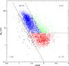 |
Fig. 1 Spectral classification diagram for the 10k high quality zCOSMOS sample. In red are passive galaxies, in blue star forming galaxies, in green red emitters. Small arrows mark objects for which we have only upper limits in EW0 [O II] . Numbers represent the fraction of objects belonging to each class. |
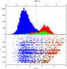 |
Fig. 2 Photometric classification of the 10k zCOSMOS-bright high quality sample. In the lower panel colour B − z versus redshift z is shown: blue triangles are star-forming, red squares are quiescent, green dots are red emitting galaxies. Solid line represents the evolutionary B − z track of a template Sab galaxy from Coleman et al. (1980) (Sawicki et al. 1997). In the upper panel the distributions of Δ(B − z), as defined in Eq. (3), for star-forming galaxies (blue histogram), quiescent galaxies (red histogram) and red emitting galaxies (green histogram) are plotted. The dashed line represents Δ(B − z) of the Sab galaxy evolutionary track used as separator. |
Figure 1 shows D4000 versus EW0 [O ii] for the “high redshift high quality” sample. The horizontal dashed line represents the cut at 5 Å in EW0 [O ii] used to separate strong and weak line emitters by M09. We used an iterative σ-clipping least squares algorithm to constrain the regions of highest density obtaining the following boundaries: ![Mathematical equation: \begin{equation} 1.64 \leq D4000 + 0.36 \log(EW_0[\ion{O}{ii}]) \leq 2.14. \end{equation}](/articles/aa/full_html/2011/11/aa16130-10/aa16130-10-eq40.png) (2)This is somewhat narrower with respect to Eq. (2) in M09, especially toward the left side of the diagram (low D4000 values) due to a lower σ rejection in the algorithm. We define star-forming galaxies as those with low values of D4000 and high values of EW0 [O ii] (66% of the galaxy sample), and quiescent galaxies (21%) as those with low values of EW0 [O ii] and high values of D4000. Galaxies populating the upper-right part of the diagram, which are 8.5% of the total, are defined as the population of intermediate galaxies with a quiescent-like continuum but strong emission lines and are mainly associated with AGNs. The black points in the left part of the diagram (4% of the total high quality sample) present uncertain spectral features and cannot be classified. Nearly 88% of the galaxies in the high-quality sample are in one of the two main classes. The “high redshift whole sample” yields a similar fraction of galaxies in each area of the D4000-EW0 [O ii] plane.
(2)This is somewhat narrower with respect to Eq. (2) in M09, especially toward the left side of the diagram (low D4000 values) due to a lower σ rejection in the algorithm. We define star-forming galaxies as those with low values of D4000 and high values of EW0 [O ii] (66% of the galaxy sample), and quiescent galaxies (21%) as those with low values of EW0 [O ii] and high values of D4000. Galaxies populating the upper-right part of the diagram, which are 8.5% of the total, are defined as the population of intermediate galaxies with a quiescent-like continuum but strong emission lines and are mainly associated with AGNs. The black points in the left part of the diagram (4% of the total high quality sample) present uncertain spectral features and cannot be classified. Nearly 88% of the galaxies in the high-quality sample are in one of the two main classes. The “high redshift whole sample” yields a similar fraction of galaxies in each area of the D4000-EW0 [O ii] plane.
3.2. Photometric classification
We introduce another classification based on the photometric properties of the galaxies. The lower panel of Fig. 2 shows the B − z colour of galaxies (Capak et al. 2007) as a function of redshift. We used the B − z colour because of its effectiveness in separating the two galaxy classes in the redshift range explored by the zCOSMOS bright sample (M09). In general, spectroscopic star-forming galaxies (blue triangles) have lower B − z and thus are bluer than both quiescent and intermediate galaxies (red squares and magenta dots respectively). As a way of discriminating the two populations we used the colour track of an Sab galaxy template from the set provided by Coleman et al. (1980, see discussion in).
We find galaxies classified as intermediate on the basis of their spectral properties are distributed in the same region as quiescent galaxies. This can be seen in the upper panel of Fig. 2, where the distribution of the distances between measured colours and the colour of the template at the redshift of the galaxy is plotted:  (3)We use the quantity Δ(B − z) to segregate the galaxies photometrically: Δ(B − z) > 0 galaxies are considered “red”, while when Δ(B − z) < 0 galaxies are put in the “blue” class. Since intermediate galaxies seem to share colours with the quiescent galaxies, we merge these spectroscopic classes into one general “quiescent” category.
Table 1 shows the 2 × 2 cross tabulation for spectral and photometric classifications. Almost 90% of the high quality sample shows full agreement between the spectral and photometric classifications (87% for the whole sample). The Cohen’s kappa coefficient for inter-rater agreement is 0.74, confirming the statistical consistency of the classifications.
Summary of the number of high spectral quality galaxies in spectroscopic and photometric classifications.
3.3. Morphological classification
Morphology data are provided by an automated code, the Zurich estimator of structural types (ZEST) (Scarlata et al. 2007), which performs a principal component analysis (PCA) of 5 quantitative morphological parameters derived directly from HST/ACS images of the COSMOS survey (Koekemoer et al. 2007).
The ZEST classification scheme adopts a main morphological index: 1 for elliptical galaxies, 2 for spirals and 3 for irregulars. In addition, a bulgeness parameter is derived from Sérsic fits (Sargent et al. 2007) to the type 2 (spiral) galaxies (see Scarlata et al. 2007, for details). They are divided into four subclasses: 2.0, 2.1, 2.2, 2.3 going from bulge-dominated spirals to disk-dominated galaxies, largely following Hubble classification of spiral galaxies from S0 through Sc types.
We assigned ZEST type 2.2, 2.3 and 3 galaxies to a common morphological category, the disk-dominated and irregular galaxies, and ZEST types 1 and 2.0 to another common category, the ellipsoidal galaxies. ZEST types 2.1 (spiral galaxies with an intermediate bulge-to-disk ratio) are sub-divided according to their colour properties. 83% ( 360 / 436) of spectroscopic star-forming galaxies of ZEST type 2.1 have a negative Δ(B − z) and are therefore classified as “blue”. A similar percentage (82%, 287 / 350) of spectroscopic quiescent galaxies of ZEST type 2.1 have Δ(B − z) > 0 and are classified as “red”. Therefore, we included the “red” population of the ZEST 2.1 type in the “ellipsoidal” morphological class and the “blue” population in the “disk-dominated” class (see discussion in M09).
In Table 3, we present the numerical results of our morphological classification. The Cohen’s kappa coefficient is ≈ 0.67 for the high quality sample, confirming a good correlation between spectroscopic and morphological parameters.
Summary of the number of high spectral quality galaxies in spectroscopic and photometric classifications.
Spectral-morphological contingency table.
3.4. The cube
To better analyse the correlations and similarities of our galaxies, we merged the three classifications (spectroscopic, photometric and morphological) into a three-axial framework, a classification cube. To simplify the classification we assigned to each galaxy a 3-digit numerical flag which encompasses information from the three categories:
-
the first digit represents the spectral classification. Flags 1 and 2 classify a galaxy as a “quiescent” and “star-forming” type, respectively;
-
the second digit stands for the colour classification. Flag 1 and 2 classify a galaxy as a “red” and “blue” type, respectively;
-
the third digit is the morphological flag. Flags 1 and 2 classify a galaxy as a “spheroidal” and “disk/irregular” type, respectively.
Table 4 shows the summary of the three-dimensional classification cube for the 4600 galaxies in common to the three classification catalogs and the 3630 galaxies in the high quality subsample. Percentages change very little between the two samples: almost 60% of the sources show a fully concordant “222” classification (star-forming spectra, blue colours, disk-dominated morphologies) and more than 20% of the sample is composed of “111” galaxies (quiescent spectra, red colours, spheroidal morphologies). On the whole, 83% of the galaxies show a fully concordant cube classification, very similar to the 85% concordance shown by the smaller zCOSMOS-bright 1k sample (see M09).
Complete classification cube.
This agreement confirms the usefulness of this kind of classification. The vast majority of galaxies in the sample belong to one of the two larger classes that show concordant behaviour in spectral, photometric and morphological properties. In these three fundamental observational features, bimodality is a major property of the galaxy population, both considering these features one at a time and comparing them in a more organic way.
4. PCA-clustering classification method
Bimodality is an intrinsic property of galaxies, not only considering single specific characteristics like colours, spectral indices, morphologies etc, but also taking those properties as a whole, as we have seen in the previous section. A classification cube stands on its own because of this global bimodality, which tells us that galaxies are well divided in two categories, “early types” and “late types”. How these two categories relate to each other is still a matter of debate, and the characterisation of transitional galaxies – objects that represent the bridge from one category to another, the so-called green valley, is of paramount importance for the definition of the evolutive history of the galaxies and to understand how and why galaxies migrate between categories.
Results of the principal component analysis applied to eight different properties of the galaxies.
For these reasons we decided to pursue a more comprehensive analysis of our sample, considering the properties of galaxies as a whole. To accomplish this task, we used statistical techniques like principal component and cluster analyses to identify the loci of early type and late type galaxies in our sample.
4.1. Principal component analysis
Principal component analysis (PCA) (Pearson 1901; Hotelling 1933) is an orthogonal linear transformation which reduces multi-dimensional data sets to fewer dimensions in order to facilitate subsequent analysis. It transforms the data to a new coordinate system such that the greatest variance in any projection of the data comes to lie on the first coordinate (called the first principal component), the second greatest variance on the second coordinate, and so on. For this reason PCA is the ideal tool to study datasets with large numbers of parameters, so as to understand their importance and correlations.
Our PCA run involved 8 observational properties of the sample: two parameters are derived from spectra (D4000 break and log (EW0 [O ii] ) – from now on we will be referring to log (EW0 [O ii] ) every time we mention the equivalent width of [O ii]; one is derived from the photometric analysis (Δ(B − z)) and the remaining parameters are morphological: M20 (second-order moment of the brightest 20% of galaxy flux, Lotz et al. 2004), concentration C (ratio between radii including 80% and 20% of galaxy light, Abraham et al. 1994; Conselice 2003), Gini coefficient G (uniformity of light distribution, Gini 1912; Lotz et al. 2004), asymmetry A (rotational symmetry of light distribution, Abraham et al. 1994, 1996) and clumpiness S (Conselice 2003), as taken from ZEST catalogue. We chose these parameters in order to keep our results comparable to the previous classification, the three-dimensional cube, which makes use of the same observables.
The result of PCA analysis applied to our set of eight normalised variables is a rotated eight-dimensional space, where every new variable PCx is a linear combination of the original ones:  (4)where − 1 ≤ a(i)x ≤ 1 are the coefficients of the linear transformation and Vi are the original variables.
In Table 5 the coefficients a(i)x of our PCA are shown. Coefficients show the relative importance of the original variables in each eigenvector PCx: the larger the value of a(i)x, the stronger the importance of the associated variable within the principal component. The two last rows of PCA table show the proportional variance (how much variance is expressed by each single PC) and the cumulative variance (how much variance is explained by the sum of the previous PCs). The three first PCs explain 84% of the original variance.
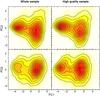 |
Fig. 3 2D density maps of the high redshift galaxies in PC1-PC2 plane (upper panels) and in PC1-PC3 plane (lower panels). Left maps are derived from the whole sample, while right ones are derived from the high quality sample only. It is clearly visible the global bimodality of galaxy properties, represented by the two “clumps” in density. |
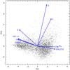 |
Fig. 4 Biplot of our PC1-PC2 plane. Black points are the galaxies as expressed in terms of PCs, while blue arrows represent the “direction” in which each original variable tends to scatter the data. |
Figure 3 shows the density of the data points in the PC1-PC2 and PC1-PC3 planes, obtained via kernel density estimation with an axis-aligned bivariate normal kernel, evaluated on a square grid (Venables & Ripley 2002). The plot shows the isodensity curves of the points, both using lines of equal density and a colour-coded 2D map: the global bimodal nature of the whole population of galaxies is reflected by the two “clumps” in density, separated by a narrow under-dense “valley”, in which transitional objects lie. The global bimodality is much more evident in the high quality sample, due to better measurements of the spectral features involved.
It is interesting to note that Disney et al. (2008) stated that only one parameter should be sufficient to describe the nature of a galaxy, although they were not able to identify it: our PCA shows that the bimodality unfolds itself in the PC1 direction alone. Although PC1 could not be that single simple parameter, it is a very interesting fact that the main properties of a galaxy can be described just by looking at its PC1 value.
The so-called biplot is a very useful tool to understand the relationships between the original variables and the PCs (Gabriel 1971), and in our work it can help explain why galaxies arrange themselves in this way in the PC space. In the biplot in Fig. 4 the arrows represent the axes where each original variable lies, and their length is an index of their “strength”, their importance within each PC – in mathematical terms the coefficients a(i)x shown in Table 5, also called loadings. Looking at the coefficients of D4000, EW0 [O ii] , Δ(B − z), G, M20 and C within PC1, for instance, one can see that they are roughly the same (in absolute value): this explains why in the biplot the relative arrows have more or less the same length along PC1 axis.
Figure 4 shows that D4000 and Δ(B − z) are strongly correlated, because the arrows point in the same direction and have similar strength. The EW0 [O ii] is anti-correlated to both of them, and this is expected given the spectral classification shown in Fig. 1; most galaxies with high values of D4000 have little or no emission lines, and vice-versa. Δ(B − z) increases with D4000, so basically redder galaxies have a larger D4000, and this is also expected from Fig. 2. We note also that C and G are strongly correlated. G is a measure of how uniformly the flux is distributed among pixels in the galaxy image, so more concentrated galaxies have a larger value of G. M20 is anti-correlated with the two other morphological parameters. Since M20 is a measure of how many bright off-centred knots of light are present, the greater is the value of M20, the “later” is the galaxy, because disk-dominated galaxies have more bright knots (star formation regions, spiral arms, bars) than spheroidal or elliptical galaxies.
Taking into consideration only PC2 we can see that asymmetry A and clumpiness S are very strongly correlated. The larger the value of PC2 for a galaxy, the more disturbed its morphology is. Objects with low values of PC2 show more regular morphologies, and are separated by their values of the other morphological parameters like C, M20 and G.
4.2. Cluster analysis
Cluster analysis is based on partitioning a collection of data points into a number of subgroups, where the objects inside a cluster show a certain degree of closeness or similarity. Hard clustering assigns each data point (feature vector) to one and only one of the clusters, with a degree of membership equal to one, and assuming well defined boundaries between the clusters. This model often does not reflect the description of real data, where boundaries between subgroups might be fuzzy, and where a more nuanced description of object’s affinity to the specific cluster is required. For this reason we applied a fuzzy clustering method to our PCA-reduced sample in order to segregate galaxies between the two clusters.
Our method makes use of the unsupervised fuzzy partition (UFP) clustering algorithm as introduced and developed by Gath & Geva (1989). The approach of this method is Bayesian: first it is required to run a partition algorithm to provide first guesses of memberships and cluster centroids. This is achieved via a modification of the fuzzy K-means algorithm (Bezdek 1973). These prototypes are then used by the second algorithm (Fuzzy modification of maximum likelihood estimation – FMLE) to achieve optimal fuzzy partition (Geva et al. 2000).
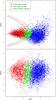 |
Fig. 5 Result of the unsupervised fuzzy partition (UFP) clustering algorithm applied to the PCA-reduced whole sample: the upper panel represents the PC1-PC2 plane, while the lower panel represents the PC1-PC3 plane. In red are early type galaxies, in blue late type galaxies, in green our intermediate objects. Brown lines are the interceptions on both planes of the 70% and 90% isoprobability surfaces. Black lines are the isodensity curves of the points in the planes, computed via Gaussian kernel smoothing. |
Figure 5 shows 2D projections of the application of the UFP clustering algorithm to our 3D dataset. The global bimodality shown by the PCA application is confirmed and well defined by the UFP algorithm. As already noted in Sect. 4.1, the leftmost objects (in red) are the early type galaxies, while in the rightmost part of the diagram (in blue) are the late type galaxies. Figure 6 shows the 3D visualization of the PC-spatial distribution of the different galaxy populations.
Since we are using a fuzzy partitioning method, objects do not belong just to one cluster: for any given data point, its probability of membership is spread across all the clusters, provided that the sum of memberships for all clusters is equal to 1.
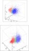 |
Fig. 6 Two different three-dimensional visualizations of the PC space. The colours represent the clusters as defined by the UFP cluster analysis in Fig. 5. Different intensities of the colours represent the distance of the point from the vantage point, trying to give the idea of the depth of the points distribution. |
Results of the principal component analysis applied to the low redshift (z < 0.48) galaxies.
In our work we assigned objects to a cluster only if their membership probability to one of the clusters is P > 0.9. We chose this threshold because, due to the exponential nature of the FMLE distance function, there is a steep rise in the probability function until P ~ 0.9, and then there is a general flattening for P ≳ 0.9. In Fig. 5 red objects are galaxies which belong to the “early type cluster” with a probability of more than 90%, while blue objects are galaxies which belong to the “late type cluster” with the same probability threshold. All other galaxies (those which belong to a cluster with a probability 0.5 < P < 0.9) are marked in green.
Early type galaxies, defined in this way, represent almost 30% of the entire sample (1413 objects), while late types are 62% (3035) and the other 8% (426) are classified as intermediate objects. The early types’ locus is more populated than the corresponding class in the classification cube (the “111” class), which consisted of 23% of the total sample (Table 4). This is due to several reasons. The 90% membership threshold for the UFP cluster analysis, which seemed a fair choice due to the shape of the probability function, is however more or less arbitrary. Choosing a 95% membership threshold, for instance, lowers the percentage of early type objects to ~20%. Moreover, the classification cube considers 8 different classes of objects, while PCA+UFP only 3 of them: many of the outliers in the classification cube (all the 121s and the 211s, and a great part of 112s and 221s) are now classified as early types in PCA+UFP. If they were to be classified as fully concordant 111s in classification cube, this class would be made up of ~31% of the whole sample. Finally, one must keep in mind that the “early type cluster”, as defined by PCA+UFP, is not intended to be made up of pure passive galaxies; but also bulge-dominated, weakly star forming objects.
Most of the differences between the two methods can be ascribed to errors and misclassifications due to the “hard partitioning” logic of the old cube classification: each of the sub-classifications of the cube were characterized by clear-cut boundaries that can produce placement errors, especially for objects that are in proximity of those boundaries. Another culprit could be the high number of morphological parameters in the PCA+UFP analysis, that might assign greater importance to those at the detriment of other parameters. However, several runs of the PCA+UFP algorithms with lower numbers of morphological parameters do not seem to substantially change the results.
Figure 5 shows the local density evaluation as shown in Fig. 3. It can be seen that the intermediate objects lie in the “valley” between the two major clumps of data points. This is expected, since we wanted to point out the relative difference between these objects and the galaxies belonging to the two clusters.
4.3. Extension to low redshifts
Due to the parameter choice of this analysis, we were forced to limit the analysis to a sub-sample of the 10k zCOSMOS sample. As we said in Sect. 2, the spectral features involved in the analysis (D4000 and EW [O ii] ) are detectable within zCOSMOS-bright only at 0.48 < z < 1.28. The higher limit in redshift coincides with the limit of the zCOSMOS-bright survey, but the nearest galaxies (between 0 < z < 0.48) were left out of the analysis. In order to expand the analysis and to follow the behaviour of galaxies in the entire redshift range of the zCOSMOS-bright survey, we decided to exploit the PCA+UFP method to probe the galaxies even at lower redshifts, substituting the spectral features used at high redshifts with one of the best star formation indicators, Hα, which is detectable within zCOSMOS-bright from the local universe to z ~ 0.48. This is one of the main reasons behind this work: the PCA+UFP method, not being tied to a particular set of data, is able to use different parameters and probe different redshift ranges and properties of the galaxies.
For the extension at low redshifts we therefore considered 7 observable parameters: Δ(B − z), M20, concentration C, Gini coefficient G, asymmetry A, clumpiness S and EW0(Hα). Like in the previous analysis with EW0 [O ii] we considered the logarithm of the equivalent width due to its log-normal distribution, so from now on EW0(Hα) has to be intended as log EW0(Hα). The low redshift sample defined in this way is composed of 3402 galaxies. Results of the application of the PCA are shown in Table 6. As for the analysis at high redshifts, we decided to consider those PCs that give a cumulative variance not less than 80%. In this case we took into account the first 4 PCs, which account for 89% of the total original variance.
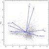 |
Fig. 7 Biplot of PC1-PC2 plane for low redshift galaxies. |
In Fig. 7 the biplot of the PCA for low redshift galaxies is shown. By comparing it with Fig. 4 one can see the striking resemblance in the cloud’s shape and in loadings’ directions. The function of D4000 and EW0 [O ii] – to segregate the galaxies mainly in PC1 direction – is taken over by EW0(Hα), while the other parameters’ relations remain largely unchanged. With respect to Fig. 4, galaxies in the early-type cluster spread more in PC2 (which is mainly morphology driven): this is probably due to ACS being progressively abler to recognise features, even in spheroidal galaxies, with decreasing redshift, due to the larger size of the galaxies themselves. So spheroidal galaxies with streams due to encounters with companions, interacting galaxies or just objects with nearby companions, have larger values of asymmetry A and clumpiness S with respect to galaxies with similar features but at higher redshifts (angular dimensions of those galaxies will be smaller and their features will most likely be too small and faint to be appreciated with an automatic analysis). This is evident in Fig. 8, where ACS snapshots of the galaxies in early types’ cluster with higher values of the second principal component (PC2 > 2) are shown.
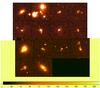 |
Fig. 8 Composite ACS image (see Koekemoer et al. 2007) of low redshift early type galaxies with highest values of PC2. Their morphologies are quite complex, suggesting tidal interactions and recent merging. |
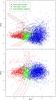 |
Fig. 9 Cluster analysis results for low redshift galaxies. Superimposed to the points, as in Fig. 5, are the isodenses of the points calculated via kernel smoothing in PC1-PC2 and PC1-PC3 planes. The curved lines represent the projected isoprobability curves. Clusters and green valley objects appear more scattered across the planes because of effects of projection from the four-dimensional PCA to the two dimensions of the plot. |
Figure 9 shows the result of the UFP clustering algorithm application to the low redshift sample of galaxies. As in previous analysis for the high redshift sample, we used a threshold of 90% membership to distinguish between objects belonging to the “early-type” cluster, to the “late-type” one or objects not belonging to any cluster – our “green valley” galaxies. Green valley objects lie in the saddle between the two main clusters, as it can be seen in the plot represented by isodensity curves, calculated by Gaussian square kernel smoothing of the PC1-PC2 and PC1-PC3 planes, in a way similar to that of the high redshift galaxies (Fig. 5). With respect to high redshift galaxies, clusters of low redshift galaxies appear less centred and defined: green dots, for instance, appear well beyond the boundaries of 90% isoprobability that define them. This is due to the isoprobability curves being merely 2D projections of 4D hypersurfaces, since, as we said, we considered the first 4 PCs for the cluster analysis.
Out of the 3402 objects in the low redshift sample, early type galaxies represent 20.6% (704 objects), while late type galaxies are 70.5% (2401), and the green valley galaxies are 8.9% (297). With respect to the high redshift sample, green valley objects represent more or less the same percentage of objects, while there is significant shift of populations between the two main clusters: late type galaxies are ~10% more with respect to the high redshift sample, while conversely early types are 10% less. This is likely to be due to a selection effect (at low redshift we are sampling galaxies with lower luminosities and lower masses, which are on average “later” at all redshifts), rather than a real evolutive feature. In the next section we will explore in more details the evolution of the galaxy populations with redshift.
5. Results
The PCA+UFP analysis presented in this work offers many improvements with respect to the previous methods of classification like the classification cube. One of the greatest advantages of such an approach is given by its self-consistency and its global approach to the parameters: as we stated in Sect. 4.2 the classification cube is prone to errors in one or more of its sub-classification methods because it uses “hard partitions”. Given the fact that every parameter is treated separately from the others, it is easier to have one of them misclassified due to internal errors, especially near the partition boundaries.
The PCA+UFP method reduces the possibility of this kind of errors because its parameters are treated simultaneously: using the PCA on a multidimensional space we are averaging over outlying values in a small number of parameters. This can be intuitively understood by looking at biplots (Figs. 4 and 7): an outlying value in M20, for instance, can be compensated by “normal” values in spectral emission lines, D4000 and C.
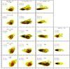 |
Fig. 10 PC1-PC2 diagrams for low redshift (upper two rows) and high redshift (lower three rows) samples, kernel smoothed with the usual technique. Columns represent bins of mass (growing from left to right, as specified inside first row boxes), while rows represent bins of redshift (growing from top to bottom, as specified in first column boxes). In each panel are also shown the absolute numbers and fractions of galaxies in each cluster (early-type, late-type and green valley), in red, blue and green respectively. In some of the high redshift panels are shown the mass completenesses (as computed by Pozzetti et al. 2010); where there are no percentages the sample has to be intended as mass-complete. |
Another powerful feature of the PCA+UFP analysis is its flexibility: due to the more or less arbitrary choice of boundaries the classification cube method described in Sect. 3 is strongly tied to its defining parameters. Replacing one or more parameters would change the very nature of the method, and human intervention would be necessary to redefine ad hoc boundaries for the new parameters. On the other side the PCA+UFP analysis is not restricted to a particular set of parameters: actually, the PCA+UFP method can successfully be applied to completely different datasets (e.g. star formation rates, masses, luminosities) of this or other galaxy surveys without requiring any adjustment by the user. In our work we extended the analysis to low redshifts just by substituting the two spectral parameters with a different one. The choice of Hα has been made in order to keep the possibility to compare the results of high and low redshift samples, and have a comprehensive look to the whole 10k dataset.
In the next subsections we will show some of the properties of the whole 10k population, and of few interesting sub-samples, in PCA+UFP analysis.
5.1. Combined high and low redshift samples
Figure 10 shows the evolution of the different populations of the 10K galaxy sample with redshift and mass. Masses have been computed by Bolzonella et al. (2010), using Bruzual & Charlot (2003) population synthesis models, by means of the Hyperzmass code, a modified version of the photo-z code Hyperz (Bolzonella et al. 2000).
Low mass galaxies (log M / M⊙ < 9.9, first column) are almost exclusively part of the late-type cluster, while high mass galaxies (log M / M⊙ > 10.7, last column) mainly belong to the early-type cluster. The transition can be mostly seen in the intermediate mass bins: at 9.9 < log M / M⊙ < 10.3, galaxies at high redshift (z > 0.80) are still forming stars actively, and are therefore concentrated in the late-type cluster. The migration towards the early type cluster seems to begin at moderately low redshifts (0.60 < z < 0.80), slowing down from z ~ 0.50 and still ongoing in the local Universe.
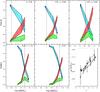 |
Fig. 11 Evolution with redshift of the fractions of different galaxy populations in mass. Each panel shows the fraction of galaxies in each mass bin that belong to each PCA+UFP cluster (in cyan are late-type galaxies, in red the early-type ones, in green the green valley ones), in a specific redshift bin. Errors are 95% confidence intervals for multinomial populations (Miller 1966). Vertical dotted lines represent the 90% mass completeness in each redshift bin. The last panel represents the evolution in z of the transition mass (Mcross), defined as the point where red line and cyan line meet (open circles and solid line). Errors associated are given by the width of the region where the two strips meet. Dashed and dot-dashed lines represent the transition masses as calculated in Pozzetti et al. (2010), respectively using Marseille morphologies and SED colours photometric classifications. The dotted line represents the transition masses as calculated using Balogh et al. (2004) definition of green valley applied to our combined sample (see Sect. 5.2). |
At slightly larger masses (10.3 < log M / M⊙ < 10.7) this transition appears to happen at earlier epochs: at 0.60 < z < 0.8 early-type and late-type galaxies are numerically comparable, and the transition appears almost complete at 0.30 < z < 0.45. At very low redshifts (z < 0.30) the percentage of late-type galaxies seems to rise again: this is most likely due to the effect of asymmetry A and clumpiness S in low-redshift ACS images we mentioned in Sect. 4.3. This delay in the star formation quenching for the lower mass galaxies, in opposition to the larger ones, can be regarded as one manifestation of the downsizing effect: the main reasons behind this effect are still unclear, even if some mechanisms have been suggested (Bower et al. 2006; Hopkins et al. 2006; Dekel & Birnboim 2006). Some numerical simulations (Schweizer 2000) show that the transition in colours should be very fast (of the order of ~500 Myr), and other observational studies seem to suggest that this is the case if the star formation is quenched efficiently; Balogh et al. (2004), however, showed that an exponentially decaying star formation can lengthen the transition phase to some Gyrs. Our work seem to suggest that a global transition (from our “late type” locus to the “early type” one) takes longer to be achieved (at least some Gyrs). Part of this is certainly due to the changes in colours and morphologies taking place with different time-scales.
Looking at Fig. 10 by rows it is possible to appreciate the mass distribution of the galaxy population at fixed redshifts. At low redshifts the zCOSMOS survey cannot sample the highest-mass galaxies (log M / M⊙ > 10.7) due to the small sampled volume and the bright magnitude cut, so the corresponding boxes are empty and were not drawn. At higher redshifts mass incompleteness prevents us from directly comparing the numbers of galaxies in each mass bin (as can be seen in the plot at z > 0.80, the mass completeness of the sample with log M / M⊙ < 9.9 is of the order of 20%). Furthermore, due to the colour dependence of the mass completeness, red galaxies are not recovered preferentially in the highest-redshift and lowest-mass bins; but as shown by e.g. Ilbert et al. (2010), in the aforementioned bins of redshift, actively star-forming galaxies are ~1 order of magnitude more abundant than the quiescent ones, therefore this mass completeness colour dependence should not constitute a significant bias. In any case, absolute numbers and fraction of galaxies in those redshift and mass bins must be taken with caution.
We summarise these considerations in Fig. 11, where each of the first five panels represents a row of Fig. 10, i.e. a bin of redshift in which we divided our sample. For every redshift bin the fraction of early type, late type and intermediate objects for each mass bin are plotted. Low mass early type galaxies are very few (~4%) in every redshift bin, late types being by far most frequent at log M / M⊙ < 9.9, which can also be seen in the first column of Fig. 10. This is in good agreement with determinations of Kovač et al. (2010) who found a similar behaviour in different environments for galaxies of different morphological type for the same zCOSMOS sample, .
Intermediate objects seem to be numerically important around log M / M⊙ ~ 10.5 at high redshifts, constituting up to ~20% of the sample at z ~ 0.5. This suggests that the evolutive transition from the blue cloud towards the red sequence may be most important at intermediate redshifts and intermediate masses (central quadrants in Fig. 10).
From Fig. 11 the masses at which early-type and late-type galaxies are numerically the same at different redshifts (Mcross), can also be derived. This transition mass, Mcross, is plotted in the lower right panel of Fig. 11 as a function of redshift. Transition masses computed in this work (solid line in the plot) are in fair agreement with those calculated by Pozzetti et al. (2010) using Marseille morphologies (Cassata et al. 2007, 2008; Tasca et al. 2009) as separators of different galaxy types – dashed line in figure – and using a photometric classification (Zucca et al. 2009) – dot-dashed line. A Cramér-von Mises test (Anderson 1962) confirms the consistency of the three estimates of Mcross (p-values above 0.73). It must be kept in mind, though, that determinations of Mcross in this work are made within a three-cluster framework (early type, late type and intermediate galaxies), while other determinations are made taking into account only the two main galaxy populations. Splitting our intermediate galaxy sample between the other two clusters, using a 50% threshold as a membership criteria, the evolution with redshift of Mcross steepens, and especially at high redshifts transition masses are even more in agreement.
The mass completeness dependence on colour discussed earlier may also play a role in the determination of Mcross as shown in Fig. 11. However, in every redshift bin Mcross lies above the 90% mass completeness limit, so its determination should be quite robust. In the redshift bins 0.60 < z < 0.80 and 0.80 < z < 1, where Mcross lies nearest to the completeness limit, even varying the fraction of early type galaxies recovered by a factor of 2, Mcross would change only by 0.1 dex.
Considering the different techniques of calculation, however, and keeping in mind the caveats, the agreement among these determinations is quite remarkable.
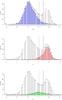 |
Fig. 12 Rest frame U − V distributions of the galaxies in the combined sample (high + low redshift). Open histograms represent the distribution of the total sample; blue, red and green histograms represent the distribution of PCA+UPF late types, early types and intermediate galaxies, respectively. Dashed lines represent green valley boundaries as defined by Balogh et al. (2004) for comparative purposes. |
5.2. Green valley galaxies
Green valley galaxies have been defined in a number of different ways, usually exploiting their natural bimodal distribution using colour indicators like u − r (Strateva et al. 2001; Baldry et al. 2004), U − V (Brown et al. 2007; Silverman et al. 2008), U − B (Vergani et al. 2010), B − i (Caputi et al. 2009). In this subsection we will analyse the U − V rest-frame colour distribution (from now on (U − V)0) of our PCA+UFP clustered galaxies.
The (U − V)0 distribution in Fig. 12, of the combined high+low redshift samples, shows a clear bimodality. The separation between the two families in colour happens at (U − V)0 ~ 1.6; the colour distribution of our late type galaxies peaks at (U − V)0 ~ 1, while the distribution of the early types is peaked at (U − V)0 ~ 1.9. All of these are in fair agreement with other determinations from literature (Silverman et al. 2008; Brammer et al. 2009). The green valley objects’ distribution peaks at (U − V)0 ~ 1.5, near the saddle of the total distribution.
We can compare the (U − V)0 distribution of our green valley galaxies with Balogh et al. (2004) definition as the 0.2mag dip between the two observed Gaussian distribution for early- and late-type galaxies. Applying the above definition to the combined sample, 760 objects out of 8256 (9.2%) would be defined as “green valley” objects. This number is very close to the number of green valley galaxies in our classification (721, 8.7%); more than 25% of our green valley objects are so also in the Balogh et al. (2004) definition, while the rest of the objects within those boundaries are almost equally divided by PCA+UFP between the two main clusters. The largest part of our intermediate galaxies lies to the left of the colour-defined green valley, i.e. in the region of the blue galaxies, but makes up only 6.5% of all the objects in that region; conversely, PCA+UFP intermediate galaxies constitute 8.4% of all the objects in the red galaxies region.
Colour selections recover no more than 25% of objects we consider intermediate. Balogh et al. shows that just two population are needed to explain the bimodalities in colour, with only ~ 1% of galaxies being in the green valley zone. However, the need for three populations in our work comes from the statistical analysis of multi-parametric spaces and cannot be directly compared with a pure colour selection. Our classification suggests that galaxies showing intermediate global properties and those in colour-defined green valley are mostly different objects.
The transition masses Mcross of the sample divided using Balogh et al. definition of green valley were also calculated (dotted line in last panel of Fig. 11). The agreement between the determinations is very high, even considering the uncertainties in the first redshift bin due to the low number of objects and the different classification schemes. Using a mass and/or redshift dependent colour definition of the green valley (e.g. Brand et al. 2009) leads to similar results.
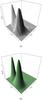 |
Fig. 13 Three dimensional representations of the high redshift galaxies density space; actual data (above) and its double bivariate Gaussian model (below). |
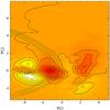 |
Fig. 14 Bidimensional density map representing residuals from the subtraction of the three-dimensional Gaussian model in Fig. 13a from the actual data density in Fig. 13b. Left side negative (light) cores and right side positive (dark) cores are due to the asymmetries in actual data densities that the model was not able to replicate. The dark core near the center of the image is due to the excess of galaxies in the saddle with respect to the Gaussian model. PCA+UFP isoprobability curves, taken from Fig. 3 are also shown. |
The presence of an intermediate third population, that arises from the PCA+UFP analysis, is also shown in Fig. 14. It represents a map of residuals from the subtraction of a double bivariate Gaussian model of the PC1-PC2 space (Fig. 13b) from the density map generated by the galaxy space (Fig. 13a – the three-dimensional equivalent of first panel in Fig. 3). The red clump near the centre of the plot represents the excess of galaxies in the saddle of the density distribution with respect to the modelled one. While it is difficult to directly compare this excess with actual galaxies (this rough analysis has been carried out in PC1-PC2 alone, while the PCA+UFP, in the high redshift range, considered three PCs), the superimposed isoprobability curves taken from Fig. 5 help visualise the position of the clump. A crude calculation on the ratio between the saddle densities allows us to estimate the objects not belonging to the tails of the two Gaussian distribution, and therefore real intermediate objects, as ≳ 80%.
5.3. Red spirals
We checked the PCA+UFP clustering properties of some of the outliers in the classification cube. Obviously this has been possible only with galaxies from the high redshift sample, because the classification cube has been defined using D4000 and EW0 [O ii] , which were available only at z > 0.48 (see Sect. 3.1). Red spirals, for instance, are often identified with edge-on spiral galaxies, reddened by a strong dust lane (Zucca et al. 2009; Tasca et al. 2009), while face-on red spirals are thought to be the very oldest spirals which used up their gas reservoirs, probably aided by strangulation and bar instabilities (Masters et al. 2010). In our classification cube, red spirals may be identified by the three-digit codes “112” and “212”, both representing morphological late-type galaxies (third digit “2”), the first one representing spectrally passive red objects and the latter one referring to red star-forming galaxies.
There are 93 galaxies with classification cube code “112” of which 24 (25.8%) are classified in the green valley group by PCA+UFP, 27 (29%) are in the late type cluster and 43 (46.2%) are in the early type cluster. A fairly high number of them (14) possess unusually high values of PC2. A visual inspection of these objects revealed very disturbed morphologies, dominated by merging and tidal streams (Fig. 8), in agreement with determinations from Conselice et al. (2000) who found that very large values of A (reflecting in our work in large values of PC2) are a good indication of ongoing major merging. At least for these objects, automatic morphological classification methods apparently fail to identify correctly them as merging spheroidals: their asymmetric characteristics are instead interpreted as late type morphologies.
74 galaxies have a classification cube code “212” of which 25 (33.8%) are classified in the green valley group, 43 (58.1%) are in the late type cluster and 6 (8.1%) are classified in the early type cluster. Their range in PC1 and PC2 is quite narrow, making these objects a rather homogeneous sample located in the middle of the PC1-PC2 diagram, in or very near the low density saddle between the clusters. These galaxies, show spiral morphologies, low star formation rates (indicated by PC1 ~ 0) and reddish colours and are the best candidates of the old spirals population mentioned by Masters et al. (2010).
5.4. Blue ellipticals
In our classification cube, blue ellipticals are identified by the three-digit codes “121” and “221”, the first one representing spectrally passive objects and the latter one referring to active star-forming galaxies, both bulge-dominated.
Classification cube code “121” galaxies are almost exclusively assigned to the early type galaxies cluster by the PCA+UFP algorithm (60/64), while code “221” show a somewhat diverse behaviour, being equally divided among the groups: 56 out of 169 (33.1%) belong to the green valley group, 52 (30.8%) to the late type cluster and 61 (36.1%) to the early type cluster. In PCA terms, objects in the latter group are characterised by positive values of PC2 and generally negative values of PC1. While code “121” galaxies are most probably the result of a colour misclassification in the classification cube, and therefore are “normal” early type galaxies – confirmed by their Δ(B − z) lying very close to the dividing line in Fig. 2 – code “221” objects seem to be more complex. Late type “221”s have large values of PC2, while the PC2 value of early type “221”s is around 0. This may imply a misclassification in Δ(B − z), too, but it is not sufficient to explain all their features. Most probably many of these objects, especially at higher values of PC1, present complex morphologies and are the result of tidal interactions.
These results seem to imply that for these objects the spectrophotometric properties are given more importance than the morphological ones by PCA+UFP algorithm. In fact, as we said, a spiral morphology classifier – especially when using wide classifiers and automatic recognition systems – is more subject to errors due to the asymmetries of merging objects.
5.5. Active galactic nuclei
We also investigated the positions, in the PCA spaces, of known AGN in the zCOSMOS sample. Type-1 AGN, which are easily recognisable by their broad emission lines and have been excluded from the samples. Type-2 AGN, on the other hand, are included in the sample since they are more difficult to identify, because their emission lines are very similar to those of regular star-forming galaxies. We used the diagnostic diagram selection of Bongiorno et al. (2010) to identify Seyfert 2 galaxies and LINERs and investigate their positions in PCA planes. Two different diagnostic diagrams have been exploited to select type-2 AGN, at low redshift using the line ratio [N ii]/Hα and [O iii]/Hβ whereas at high redshift the line ratios [O iii]/Hβ and [O ii]/Hβ have been used. Unfortunately, the different ionization properties of Seyfert 2 and LINERs galaxies are separable only using the diagnostic diagrams only at low redshifts. For this reason we will discuss the properties of the whole type-2 AGN population (which includes both active galaxy classes) in the two redshift ranges, separating the LINERs and Seyfert 2 galaxies only for z ≲ 0.5 (for a more detailed analysis see Bongiorno et al. 2010).
The analysed sample is composed by 79 type-2 AGN in the high redshift range and 125 type-2 AGN (95 of which are LINERs, while the other 30 are Seyfert 2 galaxies) in the low redshift range. Considering both the high redshift and the low redshift samples, 204 galaxies are classified as narrow line AGN: 126 (62%) are placed by PCA+UPF algorithms in the late type galaxies cluster, 47 (23%) are in the early types cluster and 31 (15%) are in the green valley region. If we restrict our analysis to the low redshift sample, 95 active galaxies are classified as LINERs: 54 (57%) are in the late types cluster, 22 (23%) are in the early types cluster and 19 (20%) are in the green valley. Conversely, the 30 pure Seyfert 2 galaxies are placed by our PCA+UPF algorithms as follows: 15 (50%) are in the late types cluster, 11 (37%) in the early types cluster and 4 (13%) in the green valley. Though we are facing small number statistics, it is clear that the majority of the type-2 AGN are hosted by galaxies which belong to the blue, late-type cluster. This is expected as our active galaxies span the low luminosity regime, as indicated by the [O iii]λ5007 Å line luminosity 105.5 L⊙ < L [O iii] < 109.1 L⊙ (Bongiorno et al. 2010).
We also explored the fraction of the selected active nuclei in the various clusters as defined by PCA+UFP with respect to the parent population of all galaxies. While the fraction of type-2 AGN in each main cluster is around 2%, this class of objects constitutes ~4% of the galaxies in the PCA+UFP green valley region. At low redshifts, LINERs represent 2% of the objects in the late type cluster and 3% of galaxies in the early type one, but they make up 6% of the green valley galaxies. This picture suggests a possible enhancement of type-2 AGN in the green valley region. However, since the numbers are small – and therefore errors are large – this might not be statistically significant. In fact, the observed type-2 AGN fractions in these subclasses are still compatible with being flat sub-samples extracted purely randomly from the parent sample.
All these classes of object do not appear to share a common locus in the PCA space, and it seems to be difficult to explain their properties with this analysis. This implies that PCA+UFP may not be the best tool to analyse outliers or particular objects, and it should be used for comprehensive population studies only.
6. Summary and conclusions
The classification cube method (Mignoli et al. 2009) has been extended and applied to the high redshift sample of the zCOSMOS-bright 10k release, exploiting bimodalites in spectral (D4000 and O ii equivalent width), photometric (B − z colour) and morphological (ZEST classification scheme) properties of the galaxies. In order to overcome some of its limitations of the classification cube (specifically the rigidity of the scheme due “hard partitioning”, the nature of misclassifications, reliance on a particular set of data and the difficulty to adopt different variables, as well as a certain degree of arbitrariness in the boundary definitions for the sub-classifications) in this work we set up a different classification method based on statistical approaches like the principal component analysis and the unsupervised fuzzy partition (PCA+UFP), that exploits the bimodal nature of galaxy properties in a more organic and rigorous way.
The PCA+UFP analysis is a very powerful and robust tool to probe the nature and the evolution of galaxies in a survey. It enables a more robust classification of galaxies, adding the flexibility to adopt different parameters. Being a fuzzy classification it avoids the problems related to a hard classification. The PCA+UFP method can be easily applied to different datasets: it does not rely on the nature of the data and for this reason it can be successfully employed with others observables (magnitudes, colours) or derived properties (masses, luminosities, SFRs, etc.).
The agreement between the two classification cluster definitions is very high. “Early” and “late” type galaxies are well defined by the spectral, photometric and morphological properties, both considering them separately and then combining the classifications (classification cube) and treating them as a whole (PCA+UFP cluster analysis). Differences arise in the definition of outliers: the classification cube is much more sensitive to single measurement errors or misclassifications in one property than the PCA+UFP cluster analysis, in which possible measurement errors are “averaged out” during the process.
The PCA+UFP analysis has also been applied to the low redshift sample, substituting D4000 and EW0 [O ii] with EW0(Hα). PCA+UFP analyses for the high and the low redshift samples clearly illustrates the effect of downsizing in the PC spaces where the migration from the blue cloud towards the red clump happens at higher redshifts for galaxies of larger mass. The determination of Mcross, the transition mass, is in good agreement with other values in literature.
The green valley objects, as defined with the PCA+UFP cluster analysis, represents a more coherent sample with respect to classical colour definitions, having the same overall physical properties. Subsequent X-ray and radio analyses could help to unveil the nature of these transitional objects.
Acknowledgments
This work was partially supported by INAF under PRIN-2006/1.06.10.08 and by ASI under grant ASI/COFIS I/016/07/0.
References
- Abraham, R. G., Valdes, F., Yee, H. K. C., & van den Bergh, S. 1994, ApJ, 432, 75 [NASA ADS] [CrossRef] [Google Scholar]
- Abraham, R. G., Tanvir, N. R., Santiago, B. X., et al. 1996, MNRAS, 279, L47 [NASA ADS] [CrossRef] [Google Scholar]
- Anderson, T. W. 1962, Ann. Math. Stat., 33, 1148 [CrossRef] [Google Scholar]
- Baldry, I. K., Glazebrook, K., Brinkmann, J., et al. 2004, ApJ, 600, 681 [NASA ADS] [CrossRef] [Google Scholar]
- Ball, N. M., Loveday, J., Brunner, R. J., Baldry, I. K., & Brinkmann, J. 2006, MNRAS, 373, 845 [NASA ADS] [CrossRef] [Google Scholar]
- Balogh, M. L., Baldry, I. K., Nichol, R., et al. 2004, ApJ, 615, L101 [NASA ADS] [CrossRef] [Google Scholar]
- Baugh, C. M., Cole, S., & Frenk, C. S. 1996, MNRAS, 283, 1361 [NASA ADS] [CrossRef] [Google Scholar]
- Bell, E. F., Wolf, C., Meisenheimer, K., et al. 2004, ApJ, 608, 752 [NASA ADS] [CrossRef] [Google Scholar]
- Bezdek, J. C. 1973, Ph.D. Thesis, Applied Math. Center, Cornell University, Ithaca [Google Scholar]
- Blanton, M. R., Hogg, D. W., Bahcall, N. A., et al. 2003, ApJ, 594, 186 [NASA ADS] [CrossRef] [Google Scholar]
- Bolzonella, M., Miralles, J., & Pelló, R. 2000, A&A, 363, 476 [NASA ADS] [Google Scholar]
- Bolzonella, M., Kovač, K., Pozzetti, L., et al. 2010, A&A, 524, A76 [NASA ADS] [CrossRef] [EDP Sciences] [Google Scholar]
- Bongiorno, A., Mignoli, M., Zamorani, G., et al. 2010, A&A, 510, A56 [NASA ADS] [CrossRef] [EDP Sciences] [Google Scholar]
- Bower, R. G., Benson, A. J., Malbon, R., et al. 2006, MNRAS, 370, 645 [NASA ADS] [CrossRef] [Google Scholar]
- Brammer, G. B., Whitaker, K. E., van Dokkum, P. G., et al. 2009, ApJ, 706, L173 [NASA ADS] [CrossRef] [Google Scholar]
- Brand, K., Moustakas, J., Armus, L., et al. 2009, ApJ, 693, 340 [NASA ADS] [CrossRef] [Google Scholar]
- Brown, M. J. I., Dey, A., Jannuzi, B. T., et al. 2007, ApJ, 654, 858 [NASA ADS] [CrossRef] [Google Scholar]
- Bruzual, A. G. 1983, ApJ, 273, 105 [NASA ADS] [CrossRef] [Google Scholar]
- Bruzual, G., & Charlot, S. 2003, MNRAS, 344, 1000 [NASA ADS] [CrossRef] [Google Scholar]
- Capak, P., Aussel, H., Ajiki, M., et al. 2007, ApJS, 172, 99 [NASA ADS] [CrossRef] [Google Scholar]
- Caputi, K. I., Lilly, S. J., Aussel, H., et al. 2009, ApJ, 707, 1387 [NASA ADS] [CrossRef] [Google Scholar]
- Cassata, P., Guzzo, L., Franceschini, A., et al. 2007, ApJS, 172, 270 [NASA ADS] [CrossRef] [Google Scholar]
- Cassata, P., Cimatti, A., Kurk, J., et al. 2008, A&A, 483, L39 [NASA ADS] [CrossRef] [EDP Sciences] [Google Scholar]
- Cimatti, A., Mignoli, M., Daddi, E., et al. 2002, A&A, 392, 395 [NASA ADS] [CrossRef] [EDP Sciences] [Google Scholar]
- Cole, S., Aragon-Salamanca, A., Frenk, C. S., Navarro, J. F., & Zepf, S. E. 1994, MNRAS, 271, 781 [NASA ADS] [CrossRef] [Google Scholar]
- Coleman, G. D., Wu, C., & Weedman, D. W. 1980, ApJS, 43, 393 [NASA ADS] [CrossRef] [Google Scholar]
- Conselice, C. J. 2003, ApJS, 147, 1 [NASA ADS] [CrossRef] [Google Scholar]
- Conselice, C. J. 2006, MNRAS, 373, 1389 [NASA ADS] [CrossRef] [Google Scholar]
- Conselice, C. J., Bershady, M. A., & Gallagher, III, J. S. 2000, A&A, 354, L21 [NASA ADS] [Google Scholar]
- Dekel, A., & Birnboim, Y. 2006, MNRAS, 368, 2 [NASA ADS] [CrossRef] [Google Scholar]
- Disney, M. J., Romano, J. D., Garcia-Appadoo, D. A., et al. 2008, Nature, 455, 1082 [NASA ADS] [CrossRef] [PubMed] [Google Scholar]
- Driver, S. P., Allen, P. D., Graham, A. W., et al. 2006, MNRAS, 368, 414 [NASA ADS] [CrossRef] [Google Scholar]
- Ellis, S. C., Driver, S. P., Allen, P. D., et al. 2005, MNRAS, 363, 1257 [NASA ADS] [CrossRef] [Google Scholar]
- Franzetti, P., Scodeggio, M., Garilli, B., et al. 2007, A&A, 465, 711 [NASA ADS] [CrossRef] [EDP Sciences] [Google Scholar]
- Gabriel, K. R. 1971, Biometrika, 58, 453 [CrossRef] [MathSciNet] [Google Scholar]
- Gath, I., & Geva, A. 1989, IEEE Transactions on Pattern Analysis and Machine Intelligence, 11, 773 [Google Scholar]
- Geva, A. B., Steinberg, Y., Bruckmair, S., & Nahum, G. 2000, Pattern Recognition Lett., 21, 511 [CrossRef] [Google Scholar]
- Gini, C. 1912, Memorie di metodologia statistica [Google Scholar]
- Hopkins, P. F., Hernquist, L., Cox, T. J., et al. 2006, ApJS, 163, 1 [Google Scholar]
- Hotelling, H. 1933, J. Educat. Psychol., 24, 417 [Google Scholar]
- Ilbert, O., Salvato, M., Le Floc’h, E., et al. 2010, ApJ, 709, 644 [NASA ADS] [CrossRef] [Google Scholar]
- Kauffmann, G., Heckman, T. M., White, S. D. M., et al. 2003, MNRAS, 341, 33 [NASA ADS] [CrossRef] [Google Scholar]
- Kauffmann, G., White, S. D. M., Heckman, T. M., et al. 2004, MNRAS, 353, 713 [NASA ADS] [CrossRef] [Google Scholar]
- Kennicutt, Jr., R. C. 1998, ARA&A, 36, 189 [Google Scholar]
- Kewley, L. J., Geller, M. J., & Jansen, R. A. 2004, AJ, 127, 2002 [NASA ADS] [CrossRef] [Google Scholar]
- Koekemoer, A. M., Aussel, H., Calzetti, D., et al. 2007, ApJS, 172, 196 [NASA ADS] [CrossRef] [Google Scholar]
- Kovač, K., Lilly, S. J., Cucciati, O., et al. 2010, ApJ, 708, 505 [NASA ADS] [CrossRef] [Google Scholar]
- Lamareille, F., Contini, T., Le Borgne, J., et al. 2006, A&A, 448, 893 [NASA ADS] [CrossRef] [EDP Sciences] [Google Scholar]
- Le Fèvre, O., Vettolani, G., Garilli, B., et al. 2005, A&A, 439, 845 [NASA ADS] [CrossRef] [EDP Sciences] [Google Scholar]
- Lilly, S. J., Le Fèvre, O., Renzini, A., et al. 2007, ApJS, 172, 70 [NASA ADS] [CrossRef] [Google Scholar]
- Lilly, S. J., Le Brun, V., Maier, C., et al. 2009, ApJS, 184, 218 [Google Scholar]
- Lotz, J. M., Primack, J., & Madau, P. 2004, AJ, 128, 163 [NASA ADS] [CrossRef] [Google Scholar]
- Marcillac, D., Elbaz, D., Charlot, S., et al. 2006, A&A, 458, 369 [NASA ADS] [CrossRef] [EDP Sciences] [Google Scholar]
- Masters, K. L., Mosleh, M., Romer, A. K., et al. 2010, MNRAS, 405, 783 [NASA ADS] [Google Scholar]
- Mignoli, M., Cimatti, A., Zamorani, G., et al. 2005, A&A, 437, 883 [NASA ADS] [CrossRef] [EDP Sciences] [Google Scholar]
- Mignoli, M., Zamorani, G., Scodeggio, M., et al. 2009, A&A, 493, 39 [NASA ADS] [CrossRef] [EDP Sciences] [Google Scholar]
- Miller, R. G. 1966, Simultaneous statistical inference (New York: McGraw-Hill), xv, 272 [Google Scholar]
- Pearson, K. 1901, Philosoph. Mag., 2, 559 [Google Scholar]
- Pozzetti, L., Bolzonella, M., Zucca, E., et al. 2010, A&A, 523, A13 [NASA ADS] [CrossRef] [EDP Sciences] [Google Scholar]
- Sargent, M. T., Carollo, C. M., Lilly, S. J., et al. 2007, ApJS, 172, 434 [NASA ADS] [CrossRef] [Google Scholar]
- Sawicki, M. J., Lin, H., & Yee, H. K. C. 1997, AJ, 113, 1 [NASA ADS] [CrossRef] [Google Scholar]
- Scarlata, C., Carollo, C. M., Lilly, S., et al. 2007, ApJS, 172, 406 [NASA ADS] [CrossRef] [Google Scholar]
-
Schweizer, F. 2000, in Roy. Soc. London Philos. Trans. Ser. A, 358, Astronomy, physics and chemistry of H
 , 2063
[Google Scholar]
, 2063
[Google Scholar]
- Silverman, J. D., Mainieri, V., Lehmer, B. D., et al. 2008, ApJ, 675, 1025 [NASA ADS] [CrossRef] [Google Scholar]
- Strateva, I., Ivezić, Ž., Knapp, G. R., et al. 2001, AJ, 122, 1861 [Google Scholar]
- Tasca, L. A. M., Kneib, J., Iovino, A., et al. 2009, A&A, 503, 379 [NASA ADS] [CrossRef] [EDP Sciences] [Google Scholar]
- Venables, W. N., & Ripley, B. D. 2002, Modern Applied Statistics with S, fourth edition (New York: Springer) [Google Scholar]
- Vergani, D., Zamorani, G., Lilly, S., et al. 2010, A&A, 509, A42 [NASA ADS] [CrossRef] [EDP Sciences] [Google Scholar]
- Zucca, E., Bardelli, S., Bolzonella, M., et al. 2009, A&A, 508, 1217 [NASA ADS] [CrossRef] [EDP Sciences] [Google Scholar]
All Tables
Summary of the number of high spectral quality galaxies in spectroscopic and photometric classifications.
Summary of the number of high spectral quality galaxies in spectroscopic and photometric classifications.
Results of the principal component analysis applied to eight different properties of the galaxies.
Results of the principal component analysis applied to the low redshift (z < 0.48) galaxies.
All Figures
|
Fig. 1 Spectral classification diagram for the 10k high quality zCOSMOS sample. In red are passive galaxies, in blue star forming galaxies, in green red emitters. Small arrows mark objects for which we have only upper limits in EW0 [O II] . Numbers represent the fraction of objects belonging to each class. |
| In the text | |
|
Fig. 2 Photometric classification of the 10k zCOSMOS-bright high quality sample. In the lower panel colour B − z versus redshift z is shown: blue triangles are star-forming, red squares are quiescent, green dots are red emitting galaxies. Solid line represents the evolutionary B − z track of a template Sab galaxy from Coleman et al. (1980) (Sawicki et al. 1997). In the upper panel the distributions of Δ(B − z), as defined in Eq. (3), for star-forming galaxies (blue histogram), quiescent galaxies (red histogram) and red emitting galaxies (green histogram) are plotted. The dashed line represents Δ(B − z) of the Sab galaxy evolutionary track used as separator. |
| In the text | |
|
Fig. 3 2D density maps of the high redshift galaxies in PC1-PC2 plane (upper panels) and in PC1-PC3 plane (lower panels). Left maps are derived from the whole sample, while right ones are derived from the high quality sample only. It is clearly visible the global bimodality of galaxy properties, represented by the two “clumps” in density. |
| In the text | |
|
Fig. 4 Biplot of our PC1-PC2 plane. Black points are the galaxies as expressed in terms of PCs, while blue arrows represent the “direction” in which each original variable tends to scatter the data. |
| In the text | |
|
Fig. 5 Result of the unsupervised fuzzy partition (UFP) clustering algorithm applied to the PCA-reduced whole sample: the upper panel represents the PC1-PC2 plane, while the lower panel represents the PC1-PC3 plane. In red are early type galaxies, in blue late type galaxies, in green our intermediate objects. Brown lines are the interceptions on both planes of the 70% and 90% isoprobability surfaces. Black lines are the isodensity curves of the points in the planes, computed via Gaussian kernel smoothing. |
| In the text | |
|
Fig. 6 Two different three-dimensional visualizations of the PC space. The colours represent the clusters as defined by the UFP cluster analysis in Fig. 5. Different intensities of the colours represent the distance of the point from the vantage point, trying to give the idea of the depth of the points distribution. |
| In the text | |
|
Fig. 7 Biplot of PC1-PC2 plane for low redshift galaxies. |
| In the text | |
|
Fig. 8 Composite ACS image (see Koekemoer et al. 2007) of low redshift early type galaxies with highest values of PC2. Their morphologies are quite complex, suggesting tidal interactions and recent merging. |
| In the text | |
|
Fig. 9 Cluster analysis results for low redshift galaxies. Superimposed to the points, as in Fig. 5, are the isodenses of the points calculated via kernel smoothing in PC1-PC2 and PC1-PC3 planes. The curved lines represent the projected isoprobability curves. Clusters and green valley objects appear more scattered across the planes because of effects of projection from the four-dimensional PCA to the two dimensions of the plot. |
| In the text | |
|
Fig. 10 PC1-PC2 diagrams for low redshift (upper two rows) and high redshift (lower three rows) samples, kernel smoothed with the usual technique. Columns represent bins of mass (growing from left to right, as specified inside first row boxes), while rows represent bins of redshift (growing from top to bottom, as specified in first column boxes). In each panel are also shown the absolute numbers and fractions of galaxies in each cluster (early-type, late-type and green valley), in red, blue and green respectively. In some of the high redshift panels are shown the mass completenesses (as computed by Pozzetti et al. 2010); where there are no percentages the sample has to be intended as mass-complete. |
| In the text | |
|
Fig. 11 Evolution with redshift of the fractions of different galaxy populations in mass. Each panel shows the fraction of galaxies in each mass bin that belong to each PCA+UFP cluster (in cyan are late-type galaxies, in red the early-type ones, in green the green valley ones), in a specific redshift bin. Errors are 95% confidence intervals for multinomial populations (Miller 1966). Vertical dotted lines represent the 90% mass completeness in each redshift bin. The last panel represents the evolution in z of the transition mass (Mcross), defined as the point where red line and cyan line meet (open circles and solid line). Errors associated are given by the width of the region where the two strips meet. Dashed and dot-dashed lines represent the transition masses as calculated in Pozzetti et al. (2010), respectively using Marseille morphologies and SED colours photometric classifications. The dotted line represents the transition masses as calculated using Balogh et al. (2004) definition of green valley applied to our combined sample (see Sect. 5.2). |
| In the text | |
|
Fig. 12 Rest frame U − V distributions of the galaxies in the combined sample (high + low redshift). Open histograms represent the distribution of the total sample; blue, red and green histograms represent the distribution of PCA+UPF late types, early types and intermediate galaxies, respectively. Dashed lines represent green valley boundaries as defined by Balogh et al. (2004) for comparative purposes. |
| In the text | |
|
Fig. 13 Three dimensional representations of the high redshift galaxies density space; actual data (above) and its double bivariate Gaussian model (below). |
| In the text | |
|
Fig. 14 Bidimensional density map representing residuals from the subtraction of the three-dimensional Gaussian model in Fig. 13a from the actual data density in Fig. 13b. Left side negative (light) cores and right side positive (dark) cores are due to the asymmetries in actual data densities that the model was not able to replicate. The dark core near the center of the image is due to the excess of galaxies in the saddle with respect to the Gaussian model. PCA+UFP isoprobability curves, taken from Fig. 3 are also shown. |
| In the text | |
Current usage metrics show cumulative count of Article Views (full-text article views including HTML views, PDF and ePub downloads, according to the available data) and Abstracts Views on Vision4Press platform.
Data correspond to usage on the plateform after 2015. The current usage metrics is available 48-96 hours after online publication and is updated daily on week days.
Initial download of the metrics may take a while.