| Issue |
A&A
Volume 533, September 2011
|
|
|---|---|---|
| Article Number | A84 | |
| Number of page(s) | 16 | |
| Section | Planets and planetary systems | |
| DOI | https://doi.org/10.1051/0004-6361/201117227 | |
| Published online | 31 August 2011 | |
Corotation torques experienced by planets embedded in weakly magnetized turbulent discs
1
DAMTP, University of Cambridge,
Wilberforce Road, Cambridge CB30,
WA,
UK
e-mail: c.baruteau@damtp.cam.ac.uk
2
Department of Astronomy and Astrophysics, University of
California, Santa
Cruz, CA
95064,
USA
3
Laboratoire AIM, CEA/DSM-CNRS-Université Paris Diderot, IRFU/SAp,
CEA/Saclay, 91191
Gif-sur-Yvette,
France
4
Astronomy Unit, Queen Mary University of London,
Mile End Road,
London
E1 4NS,
UK
5
Instituto de Ciencias Físicas, Universidad Nacional Autónoma de
México, Apdo. Postal
48-3, 62251
Cuernavaca, Morelos, México
Received:
10
May
2011
Accepted:
14
July
2011
Context. The migration of low-mass planets, or type I migration, is driven by the differential Lindblad torque and the corotation torque in non-magnetic viscous models of protoplanetary discs. The corotation torque has recently received detailed attention, because of its ability to slow down, stall, or reverse type I migration. In laminar viscous disc models, the long-term evolution of the corotation torque is intimately related to viscous and thermal diffusion processes in the planet’s horseshoe region. It is unclear how the corotation torque behaves in turbulent discs, and whether its amplitude is correctly predicted by viscous disc models.
Aims. This paper is aimed at examining the properties of the corotation torque in discs where magnetohydrodynamic (MHD) turbulence develops as a result of the magnetorotational instability (MRI), considering a weak initial toroidal magnetic field.
Methods. We present results of 3D MHD simulations carried out with two different codes. Non-ideal MHD effects and the disc’s vertical stratification are neglected, and locally isothermal disc models are considered. The running time-averaged tidal torque exerted by the disc on a fixed planet is evaluated in three different disc models.
Results. We first present simulation results with an inner disc cavity (planet trap). As in viscous disc models, the planet is found to experience a positive running time-averaged torque over several hundred orbits, which highlights the existence of an unsaturated corotation torque maintained in the long term in MHD turbulent discs. Two disc models with initial power-law density and temperature profiles are also adopted, in which the time-averaged tidal torque is found to be in decent agreement with its counterpart in laminar viscous disc models with similar viscosity alpha parameter at the planet location. Detailed analysis of the averaged torque density distributions indicates that the differential Lindblad torque takes very similar values in MHD turbulent and laminar viscous discs, and there exists an unsaturated corotation torque in MHD turbulent discs. This analysis also reveals the existence of an additional corotation torque in weakly magnetized discs.
Conclusions. Our results of 3D MHD simulations demonstrate the existence of horseshoe dynamics and an unsaturated corotation torque in weakly magnetized discs with fully developed MHD turbulence.
Key words: accretion, accretion disks / magnetohydrodynamics (MHD) / turbulence / methods: numerical / planet-disk interactions / protoplanetary disks
© ESO, 2011
1. Introduction
From the early stages of their formation, planets tidally interact with their natal protoplanetary disc. The tidal torque exerted by the disc on a planet drives the planet’s radial migration. Several migration regimes are usually distinguished, depending on the planet’s ability to clear a gap around its orbit. This ability varies with the planet-to-primary mass ratio, the disc aspect ratio (that is, the disc pressure scale height-to-radius ratio), and the disc’s turbulent viscosity (for more details, see Crida et al. 2006). The migration of planets that do not open a gap is referred to as type I migration. It typically applies to low-mass planets, up to a few Earth masses if the central object has a solar mass. In massive protoplanetary discs, intermediate-mass planets building up a partial gap (e.g., Saturn-like planets) may undergo rapid runaway migration (Masset & Papaloizou 2003). More massive planets open a clean gap and are subject to type II migration (Lin & Papaloizou 1986; Crida & Morbidelli 2007).
The reproduction of the mass-period diagram of known exoplanets by models of planet population synthesis is very sensitive to the expression for the tidal torque driving type I migration (e.g., Ida & Lin 2008a,b; Schlaufman et al. 2009; Mordasini et al. 2009). The latter has been intensively studied in two-dimensional (2D) non-magnetized, laminar viscous disc models. In such models, the torque comprises the differential Lindblad torque and the corotation torque. The differential Lindblad torque corresponds to the angular momentum carried away by the spiral density waves the planet generates in the disc, where the flow relative to the planet becomes approximately supersonic. In discs with decreasing temperature profiles, it is a negative quantity (Tanaka et al. 2002; Paardekooper et al. 2010), which, by itself, would drive type I migration on timescales shorter than a few ×105 yrs (e.g., Ward 1997). Local variations in the disc’s temperature and/or density profiles, due for example to opacity transitions (Menou & Goodman 2004) or to dust heating (Hasegawa & Pudritz 2010) may however change the sign and magnitude of the differential Lindblad torque.
The corotation torque accounts for the exchange of angular momentum between the planet and the coorbital flow. It has two components. One scales with the gradient of disc vortensity (vorticity to surface density ratio, projected along the vertical direction) across the horseshoe region (Ward 1991; Masset 2001). The other features the entropy gradient across the horseshoe region (Baruteau & Masset 2008; Paardekooper & Papaloizou 2008; Masset & Casoli 2010; Paardekooper et al. 2010). The magnitude of the corotation torque depends on the timescales for viscous and thermal diffusion inside the horseshoe region, required to maintain the local gradients of vortensity and entropy. In the absence of diffusion processes, both gradients would be progressively flattened out by advection inside the horseshoe region, and the corotation torque would ultimately vanish. This is called saturation of the corotation torque. It may be avoided by requiring that the viscous and thermal diffusion timescales across the horseshoe region be shorter than the horseshoe libration timescale (Paardekooper et al. 2011; Masset & Casoli 2010). When both diffusion timescales exceed the horseshoe U-turn timescale (a fraction of the libration timescale), the corotation torque is a non-linear process also known as horseshoe drag. When they become comparable to, or shorter than the U-turn timescale, the corotation torque decreases towards its value predicted by linear theory (Paardekooper & Papaloizou 2009), referred to as the linear corotation torque.
Depending on the disc gradients and diffusion processes at the planet orbit, the amplitude of the corotation torque can be comparable to, or larger than that of the differential Lindblad torque. The impact of the corotation torque on type I migration can therefore be of considerable importance. A lot of efforts have been recently put forward to establish simple and accurate expressions for the corotation torque as well as for the differential Lindblad torque, which can be used in population synthesis models (Masset & Casoli 2010; Paardekooper et al. 2011). These expressions were obtained for 2D non-magnetic viscous disc models.
The tidal torque has also been investigated in magnetized non-turbulent discs. The case of a 2D disc with a toroidal magnetic field has been studied by Terquem (2003) through a linear analysis. She found that the differential Lindblad torque is reduced with respect to non-magnetized discs (waves propagate outside the Lindblad resonances at the magneto-sonic speed rather than the sound speed), and that there is no linear corotation torque. Instead, angular momentum is taken away from the planet by slow MHD waves propagating in a narrow annulus near magnetic resonances. These results were confirmed by Fromang et al. (2005) with non-linear 2D MHD simulations in the regime of strong magnetic field (the plasma β-parameter was taken equal to 2 in their study, where β is the ratio of the thermal to magnetic pressures). More recently, 2D and 3D disc models with a poloidal magnetic field were investigated by Muto et al. (2008) in the shearing sheet approximation.
It is unclear how turbulence affects the tidal torque. So far, only a couple of studies have investigated this issue. Nelson & Papaloizou (2004) performed 3D simulations of locally isothermal discs fully invaded by MHD turbulence due to the MRI. They found that the running time averaged tidal torque on a fixed protoplanet experiences rather large-amplitude oscillations, and its final value quite substantially differs from the torque value expected in laminar discs. Similar results were obtained by Nelson (2005), who allowed the planet orbit to evolve. A primary reason for the observed difference between the laminar torque and the time-averaged turbulent torque is that the 3D MHD simulations were not converged in time. Baruteau & Lin (2010) considered 2D isothermal discs subject to stochastic forcing, using the turbulence model originally developed by Laughlin et al. (2004). They showed that, when time-averaged over a sufficient long time period, both the differential Lindblad torque and the corotation torque behave very similarly as in laminar viscous disc models. Uribe et al. (2011) have recently performed 3D MHD simulations of planet migration in weakly magnetized turbulent discs, including vertical stratification and a range of planet masses. For type I-migrating planets, they obtained a positive running time-averaged torque in disc models where the density near the planet’s orbital radius becomes a slightly increasing function of radius due to the disc structuring by turbulence, suggesting the existence of an unsaturated corotation torque in such disc models.
In this paper, we revisit the properties of the tidal torque experienced by a fixed planet in disc models with hydromagnetic turbulence generated by the non-linear development of the MRI. Locally isothermal discs without vertical stratification are considered, and non-ideal MHD effects are neglected. 3D MHD simulations using two different codes have been carried out, using initial values of the plasma β-parameter larger than or equal to 50. The physical model and numerical setup used in our simulations are described in Sect. 2. In Sect. 3 we present results of simulations with an inner disc cavity. In viscous disc models, an increasing density profile yields a large positive corotation torque, which may stall type I migration. This is often referred to as a planet trap (e.g., Masset et al. 2006b). Our results of turbulent simulations show a positive time-averaged tidal torque experienced by a planet fixed between the two edges of a cavity, suggesting the existence of an unsaturated corotation torque in MHD-turbulent discs. This existence is confirmed in disc models with power-law density profiles, which are described in Sect. 4. The time-averaged tidal torque obtained in such discs is in decent agreement with the torque value predicted in 2D non-magnetized viscous disc models. The discussion in Sect. 5 gives more insight into the existence of horseshoe dynamics in weakly magnetized turbulent discs, as well as a detailed comparison between the torque density distributions obtained in MHD-turbulent and laminar disc models. This comparison indicates the existence of an additional corotation torque in discs with a weak toroidal magnetic field, which will be investigated in a forthcoming study. Conclusions and future directions are drawn in Sect. 6.
2. Model description
We explore the properties of the tidal torque between a planet and its nascent protoplanetary disc, wherein turbulence is driven by the non-linear development of the MRI. A question that needs to be addressed is whether an unsaturated corotation torque exists and can be maintained in the long term in such turbulent discs. For this purpose, MHD simulations have been carried out using two different codes, which are described in Sect. 2.1. The physical model and numerical setup used in our simulations are detailed in Sect. 2.2. The parameters common to all simulations presented hereafter are listed in Table 1.
2.1. Codes
We investigate the nature of the corotation torque, a process occurring on the width of the planet’s horseshoe region that, for planets subject to type I migration, is smaller than the pressure scale height (e.g., Masset et al. 2006a). At this scale, the turbulence properties can potentially be influenced by details of the numerical scheme. Thus, we use two different codes that have different dissipation properties. This will help constrain the robustness of our results, and their limitations.
The two codes that we use to perform the 3D MHD simulations presented in this paper are NIRVANA (Ziegler & Yorke 1997) and RAMSES (Teyssier 2002; Fromang et al. 2006). NIRVANA uses an algorithm very similar to the ZEUS code to solve the equations of ideal MHD (Stone & Norman 1992). RAMSES is a finite-volume code that uses the MUSCL-Hancok Godunov scheme. For the purpose of this project, a uniform grid version of the code (i.e., without any Adaptive Mesh Refinement capabilities) was extended to allow the use of cylindrical coordinates. For comparison, results of 2D hydrodynamical simulations are also presented, performed with the codes RAMSES and FARGO (Masset 2000a,b). (None of these 2D simulations includes a magnetic field.) FARGO is very similar to the 2D hydrodynamical version of NIRVANA. Its specificity is to use a change of rotating frame on each ring of the grid, which increases the timestep significantly.
Results of simulations are expressed in the following units: the mass unit is the mass of the central star (M ⋆ ), the length unit is the planet’s (fixed) orbital separation (Rp), and the time unit is the planet’s orbital period (Torb) divided by 2π. Whenever time is expressed in orbits, it refers to the orbital period at the planet location.
2.2. Physical model and numerical setup
2.2.1. Gas disc model
We adopt a simple 3D magnetized disc model in which non-ideal MHD effects, self-gravity
and vertical stratification are neglected. No explicit kinematic viscosity is included.
The ideal MHD equations are solved in a cylindrical coordinate system
{ R,ϕ,z } centred on the central star, with
R ∈ [1;8] , ϕ ∈ [0;π] and
z ∈ [−0.3;0.3] . The frame rotates with angular frequency equal
to the Keplerian frequency at R = 3 (the fixed location of the planet,
when included), and the indirect term that accounts for the acceleration of the central
star by the planet is included in the equations of motion for those simulations that
include a planet. For simplicity, a locally isothermal equation of state is used, with
the gas pressure Pgas and mass volume density
ρ satisfying  , where the
gas sound speed cs is specified as a fixed function of
radius. It is related to the disc’s pressure scale height H through
H = cs/ΩK,
with ΩK the local Keplerian angular velocity. The disc aspect ratio,
h = H/R, is
defined to be 0.1 at R = 3. The vertical extent of the disc model is
thus equal to two pressure scale heights at the planet’s orbital radius. Ideally we
would prefer to choose a smaller disc thickness, more typical of protoplanetary disc
models. But the resolution requirement of maintaining a turbulent flow driven by the
MRI, combined with the need to run simulations for many hundreds of planet orbits, means
that we are forced to adopt a relatively thick disc model.
, where the
gas sound speed cs is specified as a fixed function of
radius. It is related to the disc’s pressure scale height H through
H = cs/ΩK,
with ΩK the local Keplerian angular velocity. The disc aspect ratio,
h = H/R, is
defined to be 0.1 at R = 3. The vertical extent of the disc model is
thus equal to two pressure scale heights at the planet’s orbital radius. Ideally we
would prefer to choose a smaller disc thickness, more typical of protoplanetary disc
models. But the resolution requirement of maintaining a turbulent flow driven by the
MRI, combined with the need to run simulations for many hundreds of planet orbits, means
that we are forced to adopt a relatively thick disc model.
The disc is set up in radial equilibrium, with the centrifugal acceleration and the radial acceleration related to the pressure gradient balancing the gravitational acceleration due to the central star (function of R only). A small level of random noise (5% of the local sound speed) is added to each component of the gas velocity. The initial radial profiles of the disc’s density and temperature will be specified in Sects. 3 and 4. The initial magnetic field is purely toroidal with a net azimuthal flux. Its radial profile is set by the choice for the plasma β-parameter, which is taken to be constant throughout the disc region in which the initial field is introduced. Several values of β in the range [50−400] are considered throughout this study, depending on the model. Their value will be specified below. The initial magnetic field is introduced everywhere except near the radial boundaries, where the field is set to zero in R ∈ [1;1.5] and R ∈ [5;8] .
The long term action of the turbulent stresses causes the disc density profile to
evolve significantly, leading eventually to most of the mass being relocated to the
close vicinity of the inner and outer radial boundaries. To avoid this and obtain a
steady-state density profile, we adopt an approach similar to that of Nelson & Gressel (2010), and reinforce the
original density profile on some specified time scale. This procedure, which we call the
mass-adding procedure for future reference, is achieved by solving 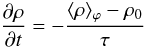 (1)alongside
the ideal MHD equations. In Eq. (1),
⟨ ρ ⟩ ϕ denotes the azimuthally-averaged
density (function of R and z),
ρ0 is the initial density (function of R
only), and τ is set to 20 local orbital periods. We checked by means of
2D hydrodynamical viscous simulations with a kinematic viscosity corresponding to a
similar amount of turbulence as in our MHD simulations that the mass-adding procedure
has a very small impact on the time evolution of the tidal torque, since the planet we
consider (see Sect. 2.2.2) does not open a gap over
the duration of our simulations. Some additional remarks on the use of the mass-adding
procedure will be made in Sect. 5.3.
(1)alongside
the ideal MHD equations. In Eq. (1),
⟨ ρ ⟩ ϕ denotes the azimuthally-averaged
density (function of R and z),
ρ0 is the initial density (function of R
only), and τ is set to 20 local orbital periods. We checked by means of
2D hydrodynamical viscous simulations with a kinematic viscosity corresponding to a
similar amount of turbulence as in our MHD simulations that the mass-adding procedure
has a very small impact on the time evolution of the tidal torque, since the planet we
consider (see Sect. 2.2.2) does not open a gap over
the duration of our simulations. Some additional remarks on the use of the mass-adding
procedure will be made in Sect. 5.3.
2.2.2. Planet parameters
We adopt a planet of mass
Mp = 3 × 10⁻⁴M ⋆ ,
which is held on a fixed circular orbit at Rp = 3,
zp = 0 (here and in the following, all quantities with the
subscript p are meant to be evaluated at the planet’s orbital radius). This corresponds
to a Saturn-mass planet if the central object is a Sun-like star. Given the large disc
aspect ratio in our model (hp = 0.1), the dimensionless
parameter determining the flow non-linearity near the planet
 . In addition, the large
turbulent stress generated by MHD turbulence (the effective viscosity parameter
α is a few percent, as we shall see in the next sections) prevents
the planet from opening a gap over the duration of our calculations (several hundred
orbits). The planet mass we consider is therefore relevant to the type I migration
regime, although it is somewhat larger than would normally be adopted in studies of the
migration of low-mass planets. The need to obtain converged estimates of the torque
experienced by the planet over runs times of several hundred planet orbits, however, has
led us to adopt this larger than preferred value. The gravitational potential of the
planet is independent of z, this being consistent with our cylindrical
disc setup. It is smoothed over a softening length, ε, equal to
0.2H(Rp). The calculation of the force
exerted by the disc on the planet excludes gas located within the planet’s Hill radius
(RH, the excluded volume is a cylinder of radius
RH centred around the planet’s position).
. In addition, the large
turbulent stress generated by MHD turbulence (the effective viscosity parameter
α is a few percent, as we shall see in the next sections) prevents
the planet from opening a gap over the duration of our calculations (several hundred
orbits). The planet mass we consider is therefore relevant to the type I migration
regime, although it is somewhat larger than would normally be adopted in studies of the
migration of low-mass planets. The need to obtain converged estimates of the torque
experienced by the planet over runs times of several hundred planet orbits, however, has
led us to adopt this larger than preferred value. The gravitational potential of the
planet is independent of z, this being consistent with our cylindrical
disc setup. It is smoothed over a softening length, ε, equal to
0.2H(Rp). The calculation of the force
exerted by the disc on the planet excludes gas located within the planet’s Hill radius
(RH, the excluded volume is a cylinder of radius
RH centred around the planet’s position).
2.2.3. Grid resolution and boundary conditions
Resolution – The grid resolution in all the
simulations presented in Sects. 3 and 4 is
(NR,Nϕ,Nz) = (320,480,40).
At the planet location, the pressure scale height is thus resolved by about 15 cells
along the radial and azimuthal directions, and by 20 cells along the vertical direction.
Since we aim to investigate the properties of the corotation torque, the radial extent
of the planet’s horseshoe region needs to be sufficiently resolved. For type I migrating
objects, its half-width, xs, is
 (e.g., Masset et al. 2006a). Here, it is resolved
by about 9 cells along the radial direction, which is similar to the resolution used in
recent studies of the corotation torque (e.g., Baruteau
& Lin 2010).
(e.g., Masset et al. 2006a). Here, it is resolved
by about 9 cells along the radial direction, which is similar to the resolution used in
recent studies of the corotation torque (e.g., Baruteau
& Lin 2010).
Azimuthal domain –
 |
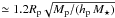
Fig. 1 Results of 2D viscous disc models with FARGO, using a constant kinematic viscosity. The steady running time-averaged specific torque on the planet (code units) is plotted against the alpha viscosity at the planet location. Results are obtained for several values of the grid’s azimuthal extent Δϕ but with the same resolution. |
As already mentioned in Sect. 2.2.1, our 3D MHD
simulations cover an azimuthal extent Δϕ = π. This
choice is the best compromise between several limitations. Having
Δϕ = 2π is a natural choice for studying the
corotation torque, and to our knowledge all works on the corotation torque have used
this azimuthal extent. But, at fixed resolution, this choice requires a maximally large
Nϕ, the number of grid cells along the
azimuthal direction. At the same resolution, decreasing Δϕ reduces
Nϕ, but at the cost of decreasing the
corotation torque. This point is illustrated in Figure 1 for 2D hydrodynamical simulations with FARGO. These simulations use the same
setup as described above for the 3D MHD simulations, except that a constant kinematic
viscosity ν is included. The initial surface density and temperature
profiles decrease as R−1/2 and
R-1, respectively. Figure 1 displays the (stationary) running time-average of the specific torque1 obtained for three series of runs with
Δϕ = π/2, π and
2π, for which
Nϕ = 240,480 and 960,
respectively. For each series, the alpha viscosity parameter at the planet location,
 ,
ranges from 6 × 10⁻⁵ to 6 × 10⁻². At a given
αp, the corotation torque can be estimated as the
difference between the total torque, and the total torque at smallest
αp (which is a good approximation for the differential
Lindblad torque; note that its value remains almost unchanged by reducing
Δϕ from 2π to
π/2). The corotation torque is approximately maximum
when the viscous diffusion timescale across the horseshoe region,
,
ranges from 6 × 10⁻⁵ to 6 × 10⁻². At a given
αp, the corotation torque can be estimated as the
difference between the total torque, and the total torque at smallest
αp (which is a good approximation for the differential
Lindblad torque; note that its value remains almost unchanged by reducing
Δϕ from 2π to
π/2). The corotation torque is approximately maximum
when the viscous diffusion timescale across the horseshoe region,
 , is
shorter than the libration timescale,
, is
shorter than the libration timescale,
 (2)but exceeds the
U-turn timescale (Baruteau & Masset 2008),
(2)but exceeds the
U-turn timescale (Baruteau & Masset 2008),
 (3)We note that, for
Δϕ = 2π, the value of αp
at which the corotation torque is maximum is in good agreement with the expression
(3)We note that, for
Δϕ = 2π, the value of αp
at which the corotation torque is maximum is in good agreement with the expression
 of Baruteau & Lin (2010), which equals
~8 × 10⁻³ for our setup. Decreasing Δϕ reduces
τlib in comparison to
τU−turn, which implies that
of Baruteau & Lin (2010), which equals
~8 × 10⁻³ for our setup. Decreasing Δϕ reduces
τlib in comparison to
τU−turn, which implies that
-
a proportionally larger viscosity is re-quired to maintain the same saturation levelof the corotation torque (that is, the same ratioτvisc/τlib);
-
the maximum amplitude of the corotation torque decreases as the ratio τlib/τU−turn approaches unity. The linear corotation torque (that is, the corotation torque in the limit of very high viscosities) is not significantly modified by reducing Δϕ.
Taking Δϕ = π is found to be a good compromise between a large enough corotation torque, easily measurable in turbulent simulations, and a tractable numerical resolution. For comparison purposes, the 2D hydrodynamical simulations presented in Sects. 3 and 4 also have Δϕ = π. In the following, time is expressed in planet orbital periods. Despite the choice for Δϕ = π, the planet’s orbital period is implicitly calculated as 2π/Ωp.
Boundary conditions – Periodic conditions are adopted at the azimuthal and vertical boundaries. The treatment of the radial boundary condition differs in the two codes. Hydrodynamic variable fluctuations are damped identically, using the scheme described in de Val-Borro et al. (2006). This scheme, which relaxes the density and velocity components towards their initial value, is applied over R ∈ [1;1.5] and R ∈ [7;8] . In order to avoid the magnetic field reaching large values near the boundaries, different strategies are used in both codes. In NIRVANA, a reflecting boundary condition is applied to the gas radial velocity that prevents the magnetic field from penetrating into the ghost zones. In RAMSES, a magnetic resistivity (η) is used in the radial buffer zones (ηin = 5 × 10⁻⁴ and ηout = 10-3 at the inner and outer boundaries, respectively). However, such an efficient field diffusion simultaneously causes the toroidal magnetic flux to escape from the grid, ultimately resulting in the volume-averaged α value decreasing with time. To avoid this effect, at each timestep, an additional axisymmetric toroidal field is added in each grid cell to guarantee that the total initial toroidal flux is conserved. In doing so, the additional toroidal field is radially distributed such that the ratio of its associated magnetic pressure and of the initial thermal pressure is uniform over the computational domain.
3. Disc model with an inner cavity
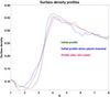 |
Fig. 2 Surface density as a function of radius shown at different times during the simulation with an inner disc cavity. |
In locally isothermal discs, the corotation torque is expected to be particularly strong in regions where the density gradient is large, and for this reason we have performed a sequence of simulations with the planet located in a disc with an inner cavity. The planet itself orbits in the transition region between the outer high-density disc and the inner low-density cavity – a region often referred to as a planet trap (Masset et al. 2006b; Morbidelli et al. 2008).
The initial disc model in this case was set up by first running a laminar disc model with
initial density and temperature profiles scaling as
R−1/2 and
R-1, respectively. The functional form for the kinematic
viscosity, ν, used to establish the cavity is 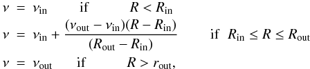 (4)with
νin = 2 × 10⁻³,
νout = νin/7,
Rin = 2.5 and Rout = 3.5. All
other parameters (e.g., grid resolution, boundary conditions) are as described in
Sect. 2. Note that the grid’s azimuthal extent equals
π in all the simulations presented from this section onwards. The
numerical simulations presented in the present section were carried out with NIRVANA.
(4)with
νin = 2 × 10⁻³,
νout = νin/7,
Rin = 2.5 and Rout = 3.5. All
other parameters (e.g., grid resolution, boundary conditions) are as described in
Sect. 2. Note that the grid’s azimuthal extent equals
π in all the simulations presented from this section onwards. The
numerical simulations presented in the present section were carried out with NIRVANA.
 |
Fig. 3 Left: volume-averaged alpha values for the disc model with an inner cavity, shown from the point in time when the planet is inserted in the disc. As in all other panels, time is expressed in orbital periods at R = 3 (the planet’s fixed location). Right: azimuthally- and vertically-averaged profiles of alpha for the same disc model, shown at different times after the planet inclusion. |
The laminar simulation was run for ~104 orbits, after which time the surface density profile had achieved the near steady-state shown by the smooth (green) curve in Fig. 2 (labelled as “Initial profile”). This profile, and the associated azimuthal velocity profile, were used to construct a 3D cylindrical disc model into which a purely toroidal magnetic field with β = 100 was introduced throughout the disc. This magnetized disc model was evolved for 76 orbits, until turbulence was fully developed throughout. The mass-adding procedure described in Sect. 2.2.1 was used to relax the density profile towards the smooth initial density profile throughout the turbulent run.
The turbulent simulation was restarted by including a planet of mass Mp = 3 × 10⁻⁴M ⋆ at R = 3. The disc-planet system was evolved for ~420 orbits. The evolution of the surface density profile (vertically-integrated density) during this time is shown in Fig. 2. Although there is a modest change in the surface density gradient at the cavity edge, due to the MHD turbulence, we see that a steep gradient is maintained. The time evolution of the volume-averaged contributions to the effective turbulent alpha viscosity (stress to thermal pressure ratios) is shown in the left panel of Fig. 3, and it is clear that these globally averaged stresses maintain a near steady-state. Snapshots of the variation of the total stress as a function of radius are shown in the right panel of Fig. 3, and again a near steady-state is observed. The effective α profile shows a maximum within the cavity, due to the low density and pressure there. A contour plot representing the disc midplane density after 127 planet orbits is displayed in Fig. 4, showing the position of the planet sitting at the edge of the cavity.
The running time-average of the torque for the turbulent disc run is shown by the red curve in Fig. 5. It remains positive, clearly indicating that the corotation torque is strong and maintained in an unsaturated state throughout the simulation. For comparison, we ran four additional 2D simulations using laminar disc models with different values of the kinematic viscosity. The initial surface density profile is the same as the initial profile shown by the green curve in Fig. 2. For comparison, the torques obtained in the 2D simulations have been multiplied by the scaling factor f = 0.6 to account for the vertical extent of the 3D simulations, where z extends from –0.3 to 0.3. We see that the laminar disc model with αp = 0.01 (shown by the green curve in Fig. 5) maintains a total torque whose cumulative time-average is similar to that of the turbulent run, but note that the surface density profiles in both runs differ about the planet location, as can be seen in Fig. 2.
The laminar run represented by the blue line in Fig. 5 adopted the kinematic viscosity profile given by Eq. (4), such that ν = 1.14 × 10⁻³ at the planet location, corresponding to the rather large value of αp ~ 0.6. The maximum unsaturated corotation torque is expected to occur when αp ~ 2 × 10⁻² (see Fig. 1), and for values larger than this, the corotation torque approaches a smaller value predicted by linear theory. Our results are consistent with this. The magenta line in Fig. 5 shows the result from a laminar simulation with αp = 10-3, a value for which we expect the corotation torque to be partially saturated. This expectation in confirmed by the simulations, and we see that the torque obtained with αp = 10-3 lies between those for αp = 0 and αp = 10-2. The black curve plotted in Fig. 5 is the torque obtained for an inviscid laminar disc. Clearly the net negative torque demonstrates that the corotation torque in this case becomes fully saturated, leaving only the differential Lindblad torque.
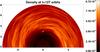 |
Fig. 4 Contours of the gas midplane density in the disc model with an inner cavity, shown 127 orbits after the planet was inserted. |
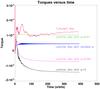 |
Fig. 5 Running time-averaged torque obtained with an inner disc cavity: comparison of laminar and turbulent disc models. |
These cavity runs show that MHD turbulence with αp ≃ 0.02 allows the corotation torque to be sustained at a value close to its maximum, unsaturated value for the disc and planet parameters that we have considered. Significant changes in the effective α, due to the turbulence being more or less vigorous, however, will cause the corotation torque to weaken. Our runs demonstrate that a planet trap maintained in a turbulent protoplanetary disc can be effective in preventing the large scale migration of embedded protoplanets.
As a conclusion to this section, our results strongly suggest the existence of an unsaturated corotation torque in turbulent protoplanetary discs with weak magnetic field (here β = 100). Although the agreement with 2D viscous laminar simulations is quite good, the complexity of the disc structure resulting from the presence and time-variation of the cavity makes it difficult to perform a quantitative analysis. The strongly increasing density profile about the planet location, the precise slope of which significantly impacts the corotation torque, and the fact the density profile can be approximated as a power-law function of R only over a limited region (≲±3H) about the planet location hinder a quantitative comparison between the torques displayed in Fig. 5 and analytic torque formulae. In Sect. 4, a suite of idealized simulations using power-law density profiles are constructed that will help study quantitatively the corotation torque properties.
4. Disc models with a power-law density profile
The results of the turbulent disc model with an inner cavity presented in Sect. 3 strongly suggest the existence of an unsaturated corotation torque in discs with hydromagnetic turbulence generated by the MRI. In the present section, we investigate the corotation torque properties in turbulent discs with initial density profiles that are power-law functions of radius. In contrast to Sect. 3, the simulations in this section have been carried out with both NIRVANA and RAMSES. A constant initial plasma β-parameter is adopted throughout the disc, which is equal to 50 in the runs performed with NIRVANA, and to 400 with RAMSES. As will be shown below, these different values are found to give similar volume-averaged alpha values in both codes.
Two disc models are considered in this section, whose parameters are summarized in Table 2. In Model 1, the initial density and temperature profiles, denoted by ρ0 and T0, decrease as R−1/2 and R-1, respectively. In Model 2, ρ0 ∝ R−3/2 and T0 is uniform. In both models, we use ρ0(R = 1) = 10-4 in code units. Assuming a Sun-like star, and that the star–planet separation is 5 AU, this corresponds to an initial surface density at the planet location ≃180 g cm-2 in Model 1, and ≃60 g cm-2 in Model 2. All other parameters are those described in Sect. 2. Recall in particular that T0(R = Rp) is chosen such that hp = 0.1. The results of both models are described in Sects. 4.1 and 4.2, respectively. In the absence of magnetic field and turbulence, the corotation torque would vanish in Model 2, but not in Model 1. However, we do not know whether and how magnetic effects modify the dependence of the corotation torque with density and temperature gradients. The tidal torque values obtained in both models can at best hint whether MHD turbulence impacts the differential Lindblad torque and the corotation torque, but they cannot allow us to work out quantitatively how each torque is altered by MHD turbulence.
4.1. Model 1: initial density ∝ R−1/2 and temperature ∝ R-1
The initial density and temperature profiles in Model 1 are the same as those of the 2D simulations of Sect. 2.2.3, where the influence of the grid’s azimuthal extent on the amplitude of the corotation torque is examined. The time evolution of the volume-averaged alpha parameter, associated with the sum of the Reynolds and Maxwell stresses, is shown in the left panel of Fig. 6. It is denoted by ⟨ αtot ⟩ . The point in time from which the planet is inserted is shown by a vertical dashed line for each simulation. The time to reach a turbulent saturated state is longer in the RAMSES run, since it uses a larger β value. In the saturated state, ⟨ αtot ⟩ ≈0.02 in both the NIRVANA and RAMSES calculations. At first, this agreement might seem surprising since the initial toroidal flux is different in the two simulations. This flux is indeed conserved throughout the simulations, and it is well known (e.g., Nelson 2005) that, in the saturated state of the turbulence, ⟨ αtot ⟩ scales with the initial toroidal flux. This agreement is in fact due to the different algorithm used by the two codes. Being less diffusive, Godunov codes are known to give in general larger alpha values (e.g., Simon et al. 2009). In this study, we tuned the respective initial toroidal fields in order to obtain the same saturated transport properties.
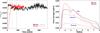 |
Fig. 6 Left: time evolution of the volume-averaged total alpha parameter, ⟨ αtot ⟩ , obtained with Model 1. Vertical dashed lines indicate the point in time when the planet is inserted in each simulation. Right: azimuthally- and vertically-averaged alpha parameters associated with the Reynolds stress (dotted curves), the Maxwell stress (dashed curves) and the total stress (solid curves) with the same model, time-averaged from 200 and 300 orbits for the simulation with RAMSES, and from 250 to 350 orbits for the simulation with NIRVANA. |
The time-averaged radial profiles of the alpha parameters associated with the Reynolds,
Maxwell and total stresses (averaged over ϕ and z) are
displayed in the right panel of Fig. 6. They are
respectively denoted by  ,
,
 and
and
 . The time average is
done between 200 and 300 orbits for the RAMSES run, and between 250 and 350 orbits for the
NIRVANA run. Note the slight decrease in both and
near the planet’s
orbital radius, which accounts for the slight increase in the disc density (or,
equivalently, the disc thermal pressure) at the same location, as shown in Fig. 7. We checked that the time-averaged magnetic stress is
slightly increased inside the planet’s Hill radius and at the location of the planet’s
wake, where the magnetic field tends to be compressed and ordered. This is reminiscent of
the findings by Nelson & Papaloizou (2003, see their Fig. 13), who however considered a
planet ~15 times more massive than ours. At the planet location,
. The time average is
done between 200 and 300 orbits for the RAMSES run, and between 250 and 350 orbits for the
NIRVANA run. Note the slight decrease in both and
near the planet’s
orbital radius, which accounts for the slight increase in the disc density (or,
equivalently, the disc thermal pressure) at the same location, as shown in Fig. 7. We checked that the time-averaged magnetic stress is
slightly increased inside the planet’s Hill radius and at the location of the planet’s
wake, where the magnetic field tends to be compressed and ordered. This is reminiscent of
the findings by Nelson & Papaloizou (2003, see their Fig. 13), who however considered a
planet ~15 times more massive than ours. At the planet location,
 .
This translates into an averaged timescale for viscous diffusion across the horseshoe
region ≃
.
This translates into an averaged timescale for viscous diffusion across the horseshoe
region ≃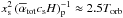 , which is similar to
the horseshoe U-turn timescale,
τU−turn ≃ 2Torb, see
Eq. (3). We thus expect the corotation
torque to adopt a value close to that predicted by linear theory.
, which is similar to
the horseshoe U-turn timescale,
τU−turn ≃ 2Torb, see
Eq. (3). We thus expect the corotation
torque to adopt a value close to that predicted by linear theory.
The time- and azimuthally-averaged disc midplane density is depicted in Fig. 7. The time-average is done over the same time interval as for the total alpha parameter shown in the right panel of Fig. 6. The mass-adding procedure described in Sect. 2.2.1, which relaxes the density profile towards its initial value over 20 local orbital periods, implies that we get a stationary density profile slightly reduced compared to the initial one, depicted by a dashed curve in Fig. 7. Note that the decrease in the disc mass is larger in the RAMSES simulation at all radii. At the planet location, the averaged-to-initial density ratio is ≈0.95 and ≈0.88 for the NIRVANA and RAMSES calculation, respectively.
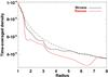 |
Fig. 7 Azimuthally- and time-averaged midplane density profile obtained in Model 1 with NIRVANA (black curve) and RAMSES (red curve). The time averaging is done between 250 and 350 orbits for the NIRVANA run, and between 200 and 300 orbits for the RAMSES run. The dashed curve displays the initial density profile common to both simulations. |
Density contours in the disc midplane obtained with the NIRVANA run after 210 orbits are
shown in Fig. 8. The planet is located at
x = 0, y = 3, and the color scale has been adjusted
such that the maximum density contour is the maximum value of the initial gas density. The
spiral density waves generated by the planet are hardly visible, their density contrast
being very similar to that of the turbulent fluctuations. Time-averaged density contours
are displayed in the left panel of Fig. 9. The time
averaging is done over 35 orbits, starting 345 orbits after the restart time (or, 520
orbits after the beginning of the simulation). This time interval corresponds to ~3
horseshoe libration periods. While the grid’s full azimuthal range is shown by the
x-axis, the y-axis displays a narrow range of radii
about the planet’s orbital radius. The planet is located at
Rp = 3 and
ϕp = π/2, and its wake
is clearly visible. Overplotted by solid lines are streamlines in the disc midplane,
evaluated from the time-averaged values of the radial and azimuthal components of the gas
velocity field over the same time interval. Horseshoe streamlines are clearly seen, which
delimit a well-defined mean horseshoe region, encompassed by mean circulating streamlines.
The use of a quite long (35 orbits) time interval for the time averaging is aimed at
displaying smooth averaged streamlines, which helps estimate the half-width of the
planet’s mean horseshoe region,  . As will be shown
in Sect. 5.1, horseshoe streamlines are readily
observed when averaging over 5 orbits (see Fig. 12).
The blue streamlines depict the approximate location of the separatrices of the mean
horseshoe region. Its half-width at
ϕ − ϕp = 1 rad is
. As will be shown
in Sect. 5.1, horseshoe streamlines are readily
observed when averaging over 5 orbits (see Fig. 12).
The blue streamlines depict the approximate location of the separatrices of the mean
horseshoe region. Its half-width at
ϕ − ϕp = 1 rad is
 . For
comparison, gas surface density contours obtained with the FARGO viscous run are shown in
the right panel of Fig. 9 along with instantaneous
streamlines. We see that the width and shape of the mean horseshoe region in the MHD
turbulent simulation are very similar to their counterpart in the laminar viscous
simulation. In the viscous run, the half-width of the horseshoe region is
xs ≈ 0.23 at
ϕ − ϕp = 1 rad. This is in good agreement
with the value obtained from the expression given by Paardekooper et al. (2010, their Eq.
(44)),
. For
comparison, gas surface density contours obtained with the FARGO viscous run are shown in
the right panel of Fig. 9 along with instantaneous
streamlines. We see that the width and shape of the mean horseshoe region in the MHD
turbulent simulation are very similar to their counterpart in the laminar viscous
simulation. In the viscous run, the half-width of the horseshoe region is
xs ≈ 0.23 at
ϕ − ϕp = 1 rad. This is in good agreement
with the value obtained from the expression given by Paardekooper et al. (2010, their Eq.
(44)), 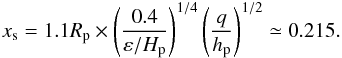 (5)
(5)
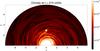 |
Fig. 8 Density contours in the disc midplane shown at 210 orbits for the NIRVANA run with Model 1. The planet is located at x = 0, y = 3. |
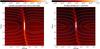 |
Fig. 9 Left: contours of the midplane density obtained in Model 1 with the NIRVANA run, and time-averaged between 520 and 555 orbits. Streamlines in the disc midplane, time-averaged over the same time interval, are overplotted by solid curves. Right: gas surface density obtained at 520 orbits with disc Model 1 in the FARGO viscous run, with instantaneous streamlines overplotted. In both panels, the horizontal dashed line shows the planet’s corotation radius, defined as the location Rc where Ω(Rc) = Ωp. |
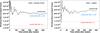 |
Fig. 10 Running time-averaged specific torque obtained with Model 1, for the NIRVANA run (left panel), and the RAMSES run (right panel). For comparison, the final value of the time-averaged torques obtained from 2D laminar disc models are overplotted, wherein the initial density profile is the time-averaged density profile obtained with the MHD run. Note that in the left panel, the turbulent run with NIRVANA is compared to laminar runs carried out with FARGO. Two series of laminar disc models have been performed, one with an inviscid disc (αp = 0), and one with a viscous disc (corresponding to αp = 0.03). |
Figure 10 depicts the running time-averaged torque (solid curves) obtained with NIRVANA (left panel) and RAMSES (right panel). We briefly recall that all torques shown in this paper refer to the specific torque exerted by the disc on the planet, and that the content of the planet’s Hill radius is excluded in the torque calculation. In both runs, the torque reaches a stationary value after typically 100 to 200 orbits. Although not shown here, this timescale is consistent with the amplitude of the stochastic torque standard deviation being similar to that of the type I migration torque in an equivalent laminar disc model (e.g., Nelson & Papaloizou 2004; Baruteau & Lin 2010). This similarity can be qualitatively expected from the similar density contrasts of the turbulent fluctuations and of the planet wake, illustrated in Fig. 8. We comment that the stationary running time-averaged torque obtained with both codes are in very good agreement, that of the RAMSES run being 10 to 20% smaller than that of the NIRVANA run. This slight difference may be (at least partly) attributed to the time-averaged density profile being slightly smaller in the RAMSES run (see Fig. 7).
How do the averaged torques of our MHD turbulent simulations compare with the predictions of laminar disc models? To address this question, we have performed two series of 2D laminar disc calculations using FARGO and RAMSES. In one series, the disc is inviscid. In the other series, a viscous disc model is used with a prescribed kinematic viscosity ν. In the latter case, the FARGO run uses a fixed radial profile for α that matches the time-averaged total alpha profile obtained in the MHD run with NIRVANA (black curve in the right panel of Fig. 6). The RAMSES run uses a constant kinematic viscosity, chosen such that αp equals the averaged alpha value obtained in the RAMSES MHD run at the planet location (≈0.03). In both series of laminar disc models, the initial density profile is the time-averaged density profile of the corresponding MHD simulations (shown in Fig. 7). We have found that the steady-state density profiles in the viscous simulations are reduced by about 10% with respect to their initial profile. At the end of the inviscid simulations (400 orbits), a tiny gap has opened about the planet’s orbital radius, with a density contrast ≃20%.
The final value of the running time-averaged torque obtained in both series of laminar calculations is overplotted in Fig. 10 by dashed lines. The 2D laminar torques have been multiplied by the scaling factor f = 0.6 to account for the vertical extent of the 3D simulations (where z ranges from −0.3 to 0.3). The torques obtained in the turbulent and viscous disc models are in good agreement, their relative difference being less than 10% for the NIRVANA and FARGO runs, and less than 20% for the RAMSES runs. Taking into account that the stationary density profile of the viscous runs is ≃10% smaller than the time-averaged density profile of the turbulent runs, the actual relative difference between the viscous and turbulent torques ranges from 20% to 30%. In the series of inviscid runs, the torque is more negative, as expected, since the (positive) corotation torque saturates after a few libration timescales, leaving only the differential Lindblad torque.
It is instructive to compare our results with the predictions of the analytical torque
expressions of Paardekooper et al. (2010), derived
for 2D viscous disc models with power-law density profiles. At the end of the inviscid
simulations, although a small gap has opened, the density profile can still be
approximated as a power-law profile. For instance, in the FARGO inviscid run, it is fairly
well approximated by
Σp(R/Rp)−1/2
with Σp ≃ 5.2 × 10⁻⁵. The torque expression in Eq. (14) of Paardekooper et al. (2010) predicts a specific
differential Lindblad torque  . Multiplying this
torque expression by the aforementioned scaling factor f gives
ΓL ≈ −1.9 × 10⁻⁵ for the density profile of the FARGO inviscid
run. This predicted value compares decently with our simulation result
(≈−1.45 × 10⁻⁵, see left panel of Fig. 10). Given the large viscosity parameter in our turbulent model, we expect that
the corotation torque is close to its linear value (Paardekooper & Papaloizou 2009). Similarly, using the parameters of the
FARGO viscous run, Paardekooper et al. (2010)
predict a linear corotation torque ≈5.6 × 10⁻⁶ (see their Eq. (16)). This is
in good agreement with our findings, where the corotation torque (estimated as the torque
of the viscous model substracted from the torque of the inviscid model) amounts to
≈6.5 × 10⁻⁶.
. Multiplying this
torque expression by the aforementioned scaling factor f gives
ΓL ≈ −1.9 × 10⁻⁵ for the density profile of the FARGO inviscid
run. This predicted value compares decently with our simulation result
(≈−1.45 × 10⁻⁵, see left panel of Fig. 10). Given the large viscosity parameter in our turbulent model, we expect that
the corotation torque is close to its linear value (Paardekooper & Papaloizou 2009). Similarly, using the parameters of the
FARGO viscous run, Paardekooper et al. (2010)
predict a linear corotation torque ≈5.6 × 10⁻⁶ (see their Eq. (16)). This is
in good agreement with our findings, where the corotation torque (estimated as the torque
of the viscous model substracted from the torque of the inviscid model) amounts to
≈6.5 × 10⁻⁶.
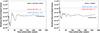 |
Fig. 11 Running time-averaged specific torque obtained in Model 2 with the NIRVANA run (left panel) and the RAMSES run (right panel). As in Fig. 10, the results of 2D inviscid and viscous disc models are overplotted, wherein the initial density profile is the time-averaged density profile of the corresponding MHD run. |
The results of this section brings more support to the existence of an unsaturated corotation torque in weakly magnetized turbulent discs. We find a decent agreement between the running time-averaged tidal torques in this particular MHD turbulent disc model, and in a viscous non-magnetic disc model with similar viscosity parameter at the planet location. The properties (shape, width) of the mean horseshoe region compare decently with those of the non-magnetic case. We cannot conclude, however, that the differential Lindblad torque and the corotation torque take similar values in both types of models. It is possible that MHD turbulence alters both the differential Lindblad torque and the corotation torque, in such a way that the total tidal torque is hardly changed. The results of Model 2, where laminar disc models predict no corotation torque, will help us evaluate to what extent MHD turbulence alters the differential Lindblad torque, and also whether or not the inclusion of magnetic effects can introduce an additional torque.
4.2. Model 2: initial density ∝ R−3/2 and uniform temperature
The results of Model 1, presented in Sect. 4.1, strongly indicate the existence of an unsaturated corotation torque in weakly magnetized turbulent discs. The tidal torque compares decently with the value expected in laminar viscous disc models. In this section, we consider a disc model with a constant temperature, and an initial density profile decreasing as R−3/2. We refer to this model as Model 2. Laminar non-magnetic disc models predict no corotation torque with such disc profiles, and that the tidal torque therefore coincides with the differential Lindblad torque. For the alpha values of our turbulent disc models (a few percent), the differential Lindblad torque is expected to have no significant dependence with the disc viscosity (e.g., Muto & Inutsuka 2009).
As in Model 1, we have carried out 2D inviscid and viscous simulations using the FARGO
and RAMSES codes. Their initial density profile is the time-averaged profile obtained in
the corresponding 3D MHD runs (that of the NIRVANA run is used as initial condition for
the 2D run with FARGO). The FARGO viscous run imposes a radial profile of alpha viscosity
equal to the radial profile  of the NIRVANA
run. In the RAMSES viscous run, a constant kinematic viscosity is used, such that the
corresponding value of αp = 0.03, the value of
⟨ αp ⟩ in the RAMSES MHD simulation.
of the NIRVANA
run. In the RAMSES viscous run, a constant kinematic viscosity is used, such that the
corresponding value of αp = 0.03, the value of
⟨ αp ⟩ in the RAMSES MHD simulation.
The time evolution of the running time-averaged torque is depicted in Fig. 11. Results with NIRVANA and FARGO are displayed in the left panel, those with RAMSES in the right panel. As in Fig. 10, the torques of the 2D runs are multiplied by the scaling factor f = 0.6, to compare them with the torques of the 3D runs. The stationary running time-averaged torques of both MHD simulations are in close agreement. This is maybe partly fortuitous, given that the corresponding time-averaged density profiles differ by about 25% (not shown here, but analogous to the different behaviors obtained in Model 1, and shown in Fig. 7). This ≃25% relative difference in density, however, is consistent with the relative difference between the torques in the laminar viscous simulations. The tiny torque difference between the inviscid and viscous runs with FARGO is most probably due to the opening of a shallow gap structure about the planet location. Gap formation also occurs in the RAMSES run, but in this particular case, it is found to have a negligible influence on the stationary running time-averaged torque.
For the parameters of Model 2, the differential Lindblad torque expression of Paardekooper et al. (2010, see their Eq. (14)) reads  . The time-averaged
density profiles of our turbulent simulations can be approximated as
Σp(R/Rp)−3/2
near the planet location, with Σp ≃ 1.9 × 10⁻⁵ and
1.6 × 10⁻⁵ for the NIRVANA and RAMSES runs, respectively. The value of
ΓL predicted by laminar disc models then amounts to about
−3.9 × 10⁻⁶ and −3.3 × 10⁻⁶ for the NIRVANA and RAMSES runs,
respectively. These predicted values agree with our numerical results to within 10% for
the NIRVANA run, and 30% for the RAMSES run.
. The time-averaged
density profiles of our turbulent simulations can be approximated as
Σp(R/Rp)−3/2
near the planet location, with Σp ≃ 1.9 × 10⁻⁵ and
1.6 × 10⁻⁵ for the NIRVANA and RAMSES runs, respectively. The value of
ΓL predicted by laminar disc models then amounts to about
−3.9 × 10⁻⁶ and −3.3 × 10⁻⁶ for the NIRVANA and RAMSES runs,
respectively. These predicted values agree with our numerical results to within 10% for
the NIRVANA run, and 30% for the RAMSES run.
The running time-averaged torque of the NIRVANA turbulent run is in reasonable agreement with the torque of the FARGO viscous run, their relative difference being about 30%. The agreement is less good for the RAMSES run, where the relative difference is ~60%. Interestingly, the averaged torque measured in both MHD simulations is more negative than in the laminar viscous runs, while the opposite trend is observed in Model 1. This comparison suggests that either the differential Lindblad torque is slightly increased, or that there exists an additional torque in magnetized turbulent discs. More insight into this hypothesis is given in Sect. 5.2.
5. Discussion
5.1. Horseshoe dynamics
Although the results presented in previous sections highlight the action of unsaturated corotation torques, we have not so far demonstrated the existence of horseshoe dynamics in our simulations without time-averaging over long timescales. A key issue is whether the horseshoe trajectories exist and can be detected easily in the presence of MHD turbulence and the associated turbulent velocity fluctuations. A related issue is the question of how rapidly the turbulence causes diffusion across the horseshoe region. This is a key factor in determining the magnitude of the corotation torque. As discussed in Sect. 2.2.3, the corotation torque in laminar viscous disc models should have its maximal non-linear value when the diffusion timescale across the horseshoe region, τvisc, is shorter than the horseshoe libration time, τlib, and is larger than the horseshoe U-turn time τU−turn ≃ hpτlib(Δϕ = 2π). If the diffusion time τvisc ≤ τU−turn, however, the corotation torque will approach the lower value expected from linear theory.
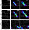 |
Fig. 12 Evolution of the concentration of the passive contaminant, C(R,ϕ), defined in the text, with superimposed averaged streamlines in the midplane for disc models with parameters equal to those of Model 1. The contour levels are defined for each panel separately to highlight the region occupied by the contaminant at each time. The upper three panels are for a disc with no embedded planet. The middle three panels have an embedded planet with Mp = 3 × 10⁻⁴ M⋆. The lower panels are for an embedded planet with Mp = 10-3 M⋆. Times are given in units of the planet orbital period. Results are obtained with NIRVANA. |
In order to examine the diffusion rate across the horseshoe region, we have performed
simulations in which a small patch of the disc in the horseshoe region is polluted
initially with a passive contaminant that is advected with the flow. We define a function
ψ(R,ϕ) = C(R,ϕ) ρ,
where C(R,ϕ) is the concentration of the contaminant,
and evolve the equation 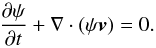 (6)We have carried
out three simulations to examine the effects of turbulent diffusion. The disc model in
each run is the same as Model 1 (see Sect. 4.1). In
the first run, no planet was included in the simulation. In the second run, a planet with
Mp = 3 × 10⁻⁴ M⋆
was included, and the system was relaxed for approximately 40 planet orbits prior to the
contaminant being introduced. In the third simulation, a Jovian mass planet with
Mp = 10-3 M⋆
was included, and a similar process of disc relaxation was undertaken to ensure that
horseshoe trajectories were fully established prior to the release of the contaminant.
(6)We have carried
out three simulations to examine the effects of turbulent diffusion. The disc model in
each run is the same as Model 1 (see Sect. 4.1). In
the first run, no planet was included in the simulation. In the second run, a planet with
Mp = 3 × 10⁻⁴ M⋆
was included, and the system was relaxed for approximately 40 planet orbits prior to the
contaminant being introduced. In the third simulation, a Jovian mass planet with
Mp = 10-3 M⋆
was included, and a similar process of disc relaxation was undertaken to ensure that
horseshoe trajectories were fully established prior to the release of the contaminant.
The results of these calculations are shown in Fig. 12, which displays contours of the contaminant concentration in the disc midplane, at three different times. The top panels show the run with no planet included. The initial patch of contaminant is located at R = 3.08, between 1.9 ≤ ϕ ≤ 2.0, and at all heights in the disc. Moving from left to right through the panels we see that the turbulence causes quite rapid diffusion in the radial direction, with the contaminant diffusing over a radial distance ≃0.2 during a time of 1.41 orbits. The Keplerian shear combines with the radial diffusion to cause the contaminant to be stretched along the azimuthal direction through advection. Nonetheless, we are able to observe that on average the initial patch of contaminant continues along its original trajectory, shearing past the nominal position of the planet that is indicated by the filled white circle. We have superimposed streamlines calculated from the time-average of the velocity field in the disc midplane over 5 orbital periods measured at R = 3 (the orbital radius of the planet, if present). As we are working in the rotating frame centred on this radius, these show the Keplerian shear for disc regions that are interior and exterior to R = 3, but it is also clear that irregular motions associated with the turbulence have not been completely averaged out over this time.
The middle panels of Fig. 12 show the run with Mp = 3 × 10⁻⁴ M⋆. It is immediately obvious that the time-averaged velocity field displays the existence of horseshoe streamlines. In general, we find that time averaging is required for temporal windows of between 3−5 orbits before the horseshoe streamlines become clearly defined in Model 1, for this planet mass. The half-width of the horseshoe region is approximately equal to 0.2, in agreement with the previous determination from the left panel of Fig. 9, where streamlines are time-averaged over 35 planet orbits.
We see that the evolution of the passive scalar is rather different from that observed in the no-planet case, and although there is significant radial diffusion we also see clear evidence of the fluid following the horseshoe streamlines. In particular, the presence of significant contaminant near the downstream inward separatrix (that is, the region bounded by 2.8 ≤ R ≤ 3 and π/2 ≤ ϕ ≤ 2) in the second and third panels demonstrates that the fluid has undergone a U-turn after approaching the planet. Similarly, at t ~ 1.81Torb, the concentration in the region bounded by 3.0 ≤ R ≤ 3.4 and 0.5 ≤ ϕ ≤ π/2 is smaller than in the no planet case. For our disc model and planet parameters, τlib ≃ 10Torb, τU−turn ≃ 2Torb, and Fig. 12 indicates that τvisc ≳ τU−turn. Note that turbulent diffusion of a passive scalar is powered by the Reynolds stress only. However, the turbulent diffusion of vortensity, which should control the magnitude of the corotation torque by analogy with viscous disc models, depends a priori both on the Reynolds and the Maxwell stresses. The timescale for turbulent diffusion of vortensity should thus be shorter than for the contaminant, and we expect the corotation torque to have a value smaller than its fully unsaturated non-linear value, in agreement with our earlier discussion of Model 1.
The lower panels of Fig. 12 show results for the run with Mp = 10-3 M⋆, and we include this simulation in our discussion only for illustration purposes. The horseshoe streamlines are now much more clearly defined, and the trajectory of the passive contaminant follows these streamlines even more clearly than in the Mp = 3 × 10⁻⁴ M⋆ run. Here, advection of the passive contaminant around the horseshoe streamlines occurs more rapidly than radial diffusion. For the time scales covered by the panels in Fig. 12, the contaminant therefore remains more or less contained within the horseshoe region.
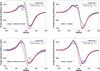 |
Fig. 13 Time average of the torque density distribution, obtained with Model 1 (top row, plus signs) and Model 2 (bottom row, plus signs). For comparison, the torque density distribution of the inviscid and viscous non-magnetic disc models are overplotted (diamond and star symbols, respectively). The torque profiles of the turbulent runs have been time-averaged over 100 orbits. In each panel, torque density profiles are divided by the maximum of the (absolute value of the) inviscid, viscous, and turbulent torque profiles. In x-axis, orbital separation is depicted from R = 2 to R = 4, which corresponds to a radial extent ≃±3Hp about the planet location. In each panel, the dashed lines show the approximate location of the separatrices of the planet’s horseshoe region, and the dotted line that of the planet’s corotation radius. |
For the disc and planet parameters of our model, we find clear evidence of the existence of horseshoe dynamics in weakly magnetized turbulent discs, in the sense that mean horseshoe streamlines are exhibited along which fluid elements perform horseshoe U-turns despite substantial turbulent diffusion. We comment that we have not shown however whether it is possible or not to get a fully unsaturated horseshoe drag in such turbulent configurations. Also, the presence of horseshoe dynamics in turbulent discs can be attributed to the averaged turbulent velocity fluctuations being of smaller amplitude than the U-turn drift rate. It is unclear whether or not a horseshoe dynamics still exists for those smaller planets for which the U-turn drift rate is smaller than the typical amplitude of the gas turbulent velocity fluctuations. This regime deserves a dedicated investigation that goes beyond the scope of this paper.
5.2. Averaged torque density distribution
The results of simulations presented in Sects. 3 and 4 support the existence of an unsaturated corotation torque in weakly magnetized turbulent discs. The running time averaged torques obtained with the NIRVANA and RAMSES codes are in very good agreement overall. Given the small scales we are interested in, this is reassuring as to the robustness of our results.
For the two disc models in Sect. 4, we find a decent agreement overall between the steady running time-averages of the tidal torque in the turbulent and viscous simulations. In Model 1, the torque relative difference between turbulent and viscous models is less than 30% for both codes. In Model 2, however, it is less than 60%. To provide more insight into these torque differences, we compare in Fig. 13 the time-averaged torque density profiles obtained for both models (depicted by plus symbols), with the torque density profiles of the viscous and inviscid laminar disc models (star and diamond symbols, respectively). Results with FARGO and NIRVANA are shown in the left panel, those with RAMSES in the right panel. The torque profiles of the MHD runs are time-averaged over 100 orbits. In each plot, the approximate location of the separatrices of the planet’s horseshoe region is indicated by dashed lines.
We first compare the torque density distributions obtained in the laminar disc models. In Model 1, the torque distributions of the viscous and inviscid runs mostly differ within the planet’s horseshoe region. This difference highlights the positive unsaturated corotation torque of the viscous disc model. Slight differences can be noticed between the corotation torque distributions of the FARGO and RAMSES simulations. In Model 2, where there is no corotation torque, the torque distributions of the viscous and inviscid simulations are in very good agreement. Their tiny differences show the influence of viscous diffusion on the radial profile of the differential Lindblad torque.
We now compare the averaged torque distribution of the MHD runs (plus symbols) with the torque distribution of the viscous runs (star symbols). Outside the planet’s (mean) horseshoe region, both distributions are found to be in overall good agreement. This is a clear demonstration that the differential Lindblad torque remains essentially unchanged by the full development of MHD turbulence. Inside the planet’s horseshoe region, however, differences are significant. In Model 2, the turbulent torque distribution takes more negative values over most of the horseshoe region, except near the outer separatrix, where it takes more positive values. Note the excellent agreement between the turbulent torque distributions of the NIRVANA and RAMSES runs. In contrast, the turbulent torque distribution obtained in Model 1 tends to take more positive values over the horseshoe region, except near the inner separatrix, although this trend is less evident in the RAMSES run. These torque differences suggest the existence of an additional torque in weakly magnetized turbulent discs that originates from the planet’s horseshoe region. The distribution of this additional torque, in particular its asymmetry, accounts for the torque differences between the MHD turbulent and viscous simulations underlined in Sects. 4.1 and 4.2.
It is quite surprising that the density distribution of the additional torque is not symmetric with respect to the location of the planet, or of the planet’s corotation radius. This offset is obtained with our two codes, but it differs in Models 1 and 2. Notwithstanding the offset, both models point out that the additional torque tends to take negative values in the inner half of the horseshoe region, and positive values in the outer half. This suggests that the additional torque is probably not powered by magnetic resonances. As shown by Terquem (2003), the torques at the magnetic and Lindblad resonances have the same sign. The torque exerted by the disc on the planet near the inner (outer) magnetic resonance is therefore positive (negative) (see also Fromang et al. 2005, their Fig. 6). The torque distribution of this so-called magnetic torque, and of the additional torque in our magnetized turbulent disc models, therefore have opposite signs. We also point out that magnetic resonances are barely resolved in our setup. Their location, Rm, as given by linear theory (Terquem 2003), satisfies |Rm − Rp| = (2Hp/3)(1 + β)−1/2, with β the effective plasma parameter evaluated from the average of the magnetic field squared. For the NIRVANA runs, we find β ≈ 40, and |Rm − Rp| ≈ 0.03 is scarcely larger than our mesh size (≈0.02).
It is possible that the additional torque found in our magnetized turbulent disc models is an additional corotation torque. Neglecting turbulence for the time being, in a magnetized disc with a purely toroidal magnetic field the magnetic tension tries to prevent radial motion associated with horseshoe U-turns imposed by the planet’s gravity, and attempts to force fluid element trajectories to follow field lines. When the magnetic field is strong enough, it is conceivable that magnetic tension can prevent horseshoe U-turns, cancelling the corotation torque. This might explain why the torque distribution in the 2D MHD simulations of Fromang et al. (2005), where β = 2, reveals no corotation torque, but instead a magnetic torque with properties similar to those predicted by linear theory. However, a weak magnetic field, such as the one we consider here, cannot prevent horseshoe U-turns, as we have demonstrated in Sect. 5.1. In this case, we speculate that magnetic tension will lead to asymmetric horseshoe U-turns, with downstream streamlines being closer to the corotation radius than the upstream streamlines. This is equivalent to saying that fluid elements in weakly magnetized discs will experience smaller changes to their angular momenta during horseshoe U-turns than they will in non-magnetized discs, with a consequence being that the density near the downstream separatrices will be reduced. Magnetic tension will thus reduce the positive corotation torque on the planet arising from fluid elements undergoing inward horseshoe U-turns, and will reduce the magnitude of the negative corotation torque arising from fluid elements undergoing outward horseshoe U-turns. This predicted behaviour is in broad agreement with the results presented in Fig. 13, provided we ignore the fact that the modification to the corotation torque observed in the simulations is not quite symmetric about the corotation radius. The origin of this offset about the corotation radius is not understood at present. A more detailed investigation of horseshoe dynamics in the presence of a weak toroidal magnetic field and MHD turbulence goes beyond the scope of this work, however, and will be presented in a forthcoming publication.
We finally comment that the results of this study have been obtained with rather large values of the disc aspect ratio (hp = 0.1) and of the planet mass (Mp = 3 × 10⁻⁴ M⋆). Although this planet mass is relevant to type I migration (see Sect. 2.2.2), it is a priori not straightforward to adapt our results to smaller, more canonical values of hp and Mp, or to different values of the alpha viscosity parameter associated with the turbulent stress. This requires knowledge of the properties of the total corotation torque in laminar magnetized discs, and whether or not they are altered by MHD turbulence.
5.3. Mass-adding procedure
The MHD simulations presented in this study were carried out using the mass-adding procedure described in Sect. 2.2.1. This procedure, which restores the initial density profile on a timescale set to 20 orbital periods, aims at obtaining a steady-state density profile, mass being otherwise continuously relocated by the turbulence towards the radial boundaries of the computational domain. Not including this procedure would make both the density profile and the running time-averaged tidal torque non-stationary quantities. In the simulations presented in Sect. 4, the choice for a restoring timescale of 20 orbital periods helps obtain a time-averaged density profile close to the initial profile, and which can be approximated as a power-law function of radius over a rather large radial extent about the planet’s orbital radius (see Fig. 7). This has enabled us to compare the torques of our simulations with analytical torque formulae derived in disc models with power-law density profiles. A different restoring timescale would result in a different density profile in a steady-state, and therefore in a different tidal torque. Although not presented here, we performed another MHD simulation with the parameters of Model 1 and a restoring timescale increased to 40 orbital periods. This additional run was performed with the NIRVANA code. We also carried out an additional 2D viscous simulation using the FARGO code, where the initial profiles of the density and of the viscous alpha parameter correspond to their time-averaged counterpart in the MHD simulation (this is the same approach as that adopted in Sect. 4). The agreement between the laminar and turbulent simulations is very similar to that obtained with a restoring timescale of 20 orbital periods: the time-averaged turbulent and laminar torques agree to within ~10%, and the torque density distributions show the same features as in the top-left panel of Fig. 13. This agreement makes us confident that the mass-adding procedure does not introduce any other artifacts on the time-averaged tidal torque than the one naturally arising from changing the density profile in a steady-state by choosing a different restoring timescale. We finally stress that this procedure should not be used in turbulent disc models involving a gap-opening planet.
6. Conclusions
In this paper we have investigated the tidal torque between a planet on a fixed circular orbit and its nascent protoplanetary disc, assuming that the latter sustains turbulence driven by the non-linear development of the MRI. Our main aim has been to investigate the properties of the corotation torque in such turbulent discs. In this initial study, we adopted simple 3D magnetized disc models with a locally isothermal equation of state, and neglected vertical stratification and non-ideal MHD effects. We performed simulations using two different MHD codes (NIRVANA and RAMSES) over time spans of several hundred planet orbits.
In one set of simulations, we considered the torque experienced by a planet orbiting at the outer edge of an inner disc cavity, in a region with a strong, positive density gradient. The running time-averaged torque in this case was found to be strongly positive over several hundred planet orbits, in good agreement with the results of laminar viscous disc simulations whose viscous stresses were similar to that generated by the MHD turbulence. This positive torque strongly suggests the existence of an unsaturated corotation torque in weakly magnetized turbulent disc models. It implies that the presence of an inner cavity can stall type I migration, such that a planet trap can operate in turbulent discs.
We also performed simulations of two disc models with power-law initial density profiles. We found that the running time-averaged torque of the turbulent disc models reached a stationary value after 100 to 200 planet orbits, with decent agreement between it and a laminar viscous disc model with similar viscous alpha parameter at the planet location. The relative difference between the averaged torques in turbulent and laminar disc simulations ranges from 20% to 60%, depending on the code and the disc model. We find remarkably good overall agreement between the results of the two codes, and given the scales of interest (the half-width of the planet’s horseshoe region is a fraction of the pressure scale height), this agreement highlights the robustness of our results.
Analysis of the velocity fields in our simulations shows the existence of horseshoe dynamics in turbulent discs with a weak toroidal magnetic field. The shape and width of the time-averaged horseshoe region much resemble those of laminar viscous discs with similar viscosity at the planet’s location. Furthermore, close inspection of the averaged torque density distributions demonstrates that the differential Lindblad torque takes very similar values in turbulent and laminar viscous disc models, and there exists an unsaturated corotation torque in weakly magnetized turbulent discs. This analysis, however, also indicates the existence of an additional torque with respect to the non-magnetic case, which originates from the planet’s horseshoe region. We argue that this additional torque is likely to be an additional corotation torque, possibly arising from the effects of magnetic tension.
Although we have demonstrated conclusively the existence of unsaturated corotation torques in weakly magnetized turbulent discs, our study contains a number of simplifications that need to be addressed. We have considered disc and planet parameters such that the horseshoe U-turn drift rate exceeds the amplitude of the turbulent velocity fluctuations. In the opposite case, the existence of horseshoe dynamics and a corotation torque is unknown. We have neglected vertical stratification and non-ideal MHD effects such as Ohmic resistivity, and it is fully expected that inclusion of these effects will modify the results presented here. We have also kept the planet on a fixed circular orbit and simply measured the tidal torque as a time series. In reality the planet will migrate and experience evolution in its eccentricity and inclination as a result of interaction with the turbulent disc. We will address these issues in a series of forthcoming publications, along with an in-depth investigation of the additional corotation torque in weakly magnetized discs that our simulations have uncovered.

Acknowledgments
C.B. acknowledges support from a Herchel Smith Postdoctoral Fellowship. S.F. acknowledges the help of Edouard Audit in extending RAMSES to cylindrical coordinates systems. The simulations performed with RAMSES were granted access to the HPC resources of CCRT and CINES under the allocation x2010042231 made by GENCI (Grand Equipement National de Calcul Intensif). Simulations with NIRVANA and FARGO were carried out on the Pleiades Cluster at U. C. Santa Cruz, on the Darwin Supercomputer of the University of Cambridge High Performance Computing Service (http://www.hpc.cam.ac.uk), provided by Dell Inc. using Strategic Research Infrastructure Funding from the Higher Education Funding Council for England. NIRVANA simulations were also performed on the QMUL HPC facilities purchased under the SRIF/CIF initiatives. This research was initiated during the Isaac Newton Institute programme “Dynamics of Discs and Planets”. We thank J. Guilet and J. Papaloizou for useful discussions, and A. Uribe, the referee, for a prompt and useful report.
References
- Baruteau, C., & Lin, D. N. C. 2010, ApJ, 709, 759 [NASA ADS] [CrossRef] [Google Scholar]
- Baruteau, C., & Masset, F. 2008, ApJ, 672, 1054 [NASA ADS] [CrossRef] [Google Scholar]
- Crida, A., & Morbidelli, A. 2007, MNRAS, 377, 1324 [NASA ADS] [CrossRef] [Google Scholar]
- Crida, A., Morbidelli, A., & Masset, F. 2006, Icarus, 181, 587 [Google Scholar]
- de Val-Borro, M., Edgar, R. G., Artymowicz, P., et al. 2006, MNRAS, 370, 529 [NASA ADS] [CrossRef] [Google Scholar]
- Fromang, S., Terquem, C., & Nelson, R. P. 2005, MNRAS, 363, 943 [NASA ADS] [CrossRef] [Google Scholar]
- Fromang, S., Hennebelle, P., & Teyssier, R. 2006, A&A, 457, 371 [NASA ADS] [CrossRef] [EDP Sciences] [Google Scholar]
- Hasegawa, Y., & Pudritz, R. E. 2010, ApJ, 710, L167 [NASA ADS] [CrossRef] [Google Scholar]
- Ida, S., & Lin, D. N. C. 2008a, ApJ, 673, 487 [NASA ADS] [CrossRef] [Google Scholar]
- Ida, S., & Lin, D. N. C. 2008b, ApJ, 685, 584 [NASA ADS] [CrossRef] [Google Scholar]
- Laughlin, G., Steinacker, A., & Adams, F. C. 2004, ApJ, 608, 489 [NASA ADS] [CrossRef] [Google Scholar]
- Lin, D. N. C., & Papaloizou, J. 1986, ApJ, 309, 846 [NASA ADS] [CrossRef] [Google Scholar]
- Masset, F. 2000a, A&AS, 141, 165 [NASA ADS] [CrossRef] [EDP Sciences] [Google Scholar]
- Masset, F. S. 2000b, in Disks, Planetesimals, and Planets, ed. G. Garzón, C. Eiroa, D. de Winter, & T. J. Mahoney, ASP Conf. Ser., 219, 75 [Google Scholar]
- Masset, F. S. 2001, ApJ, 558, 453 [Google Scholar]
- Masset, F. S., & Casoli, J. 2010, ApJ, 723, 1393 [NASA ADS] [CrossRef] [Google Scholar]
- Masset, F. S., & Papaloizou, J. C. B. 2003, ApJ, 588, 494 [NASA ADS] [CrossRef] [Google Scholar]
- Masset, F. S., D’Angelo, G., & Kley, W. 2006a, ApJ, 652, 730 [NASA ADS] [CrossRef] [Google Scholar]
- Masset, F. S., Morbidelli, A., Crida, A., & Ferreira, J. 2006b, ApJ, 642, 478 [NASA ADS] [CrossRef] [Google Scholar]
- Menou, K., & Goodman, J. 2004, ApJ, 606, 520 [NASA ADS] [CrossRef] [Google Scholar]
- Morbidelli, A., Crida, A., Masset, F., & Nelson, R. P. 2008, A&A, 478, 929 [NASA ADS] [CrossRef] [EDP Sciences] [Google Scholar]
- Mordasini, C., Alibert, Y., Benz, W., & Naef, D. 2009, A&A, 501, 1161 [NASA ADS] [CrossRef] [EDP Sciences] [Google Scholar]
- Muto, T., & Inutsuka, S. 2009, ApJ, 701, 18 [NASA ADS] [CrossRef] [Google Scholar]
- Muto, T., Machida, M. N., & Inutsuka, S.-I. 2008, ApJ, 679, 813 [NASA ADS] [CrossRef] [Google Scholar]
- Nelson, R. P. 2005, A&A, 443, 1067 [NASA ADS] [CrossRef] [EDP Sciences] [Google Scholar]
- Nelson, R. P., & Gressel, O. 2010, MNRAS, 409, 639 [NASA ADS] [CrossRef] [Google Scholar]
- Nelson, R. P., & Papaloizou, J. C. B. 2003, MNRAS, 339, 993 [NASA ADS] [CrossRef] [MathSciNet] [Google Scholar]
- Nelson, R. P., & Papaloizou, J. C. B. 2004, MNRAS, 350, 849 [NASA ADS] [CrossRef] [Google Scholar]
- Paardekooper, S.-J., & Papaloizou, J. C. B. 2008, A&A, 485, 877 [NASA ADS] [CrossRef] [EDP Sciences] [Google Scholar]
- Paardekooper, S.-J., & Papaloizou, J. C. B. 2009, MNRAS, 394, 2283 [NASA ADS] [CrossRef] [Google Scholar]
- Paardekooper, S., Baruteau, C., Crida, A., & Kley, W. 2010, MNRAS, 401, 1950 [NASA ADS] [CrossRef] [Google Scholar]
- Paardekooper, S., Baruteau, C., & Kley, W. 2011, MNRAS, 410, 293 [NASA ADS] [CrossRef] [Google Scholar]
- Schlaufman, K. C., Lin, D. N. C., & Ida, S. 2009, ApJ, 691, 1322 [NASA ADS] [CrossRef] [Google Scholar]
- Simon, J. B., Hawley, J. F., & Beckwith, K. 2009, ApJ, 690, 974 [NASA ADS] [CrossRef] [Google Scholar]
- Stone, J. M., & Norman, M. L. 1992, ApJS, 80, 753 [Google Scholar]
- Tanaka, H., Takeuchi, T., & Ward, W. R. 2002, ApJ, 565, 1257 [NASA ADS] [CrossRef] [Google Scholar]
- Terquem, C. E. J. M. L. J. 2003, MNRAS, 341, 1157 [NASA ADS] [CrossRef] [Google Scholar]
- Teyssier, R. 2002, A&A, 385, 337 [NASA ADS] [CrossRef] [EDP Sciences] [Google Scholar]
- Uribe, A., Klahr, H., Flock, M., & Henning, T. 2011, ApJ, 736, 85 [NASA ADS] [CrossRef] [Google Scholar]
- Ward, W. R. 1991, in Lunar and Planetary Institute Conference Abstracts, 1463 [Google Scholar]
- Ward, W. R. 1997, Icarus, 126, 261 [NASA ADS] [CrossRef] [Google Scholar]
- Ziegler, U., & Yorke, H. W. 1997, Comp. Phys. Comm., 101, 54 [Google Scholar]
All Tables
All Figures
|
Fig. 1 Results of 2D viscous disc models with FARGO, using a constant kinematic viscosity. The steady running time-averaged specific torque on the planet (code units) is plotted against the alpha viscosity at the planet location. Results are obtained for several values of the grid’s azimuthal extent Δϕ but with the same resolution. |
| In the text | |
|
Fig. 2 Surface density as a function of radius shown at different times during the simulation with an inner disc cavity. |
| In the text | |
|
Fig. 3 Left: volume-averaged alpha values for the disc model with an inner cavity, shown from the point in time when the planet is inserted in the disc. As in all other panels, time is expressed in orbital periods at R = 3 (the planet’s fixed location). Right: azimuthally- and vertically-averaged profiles of alpha for the same disc model, shown at different times after the planet inclusion. |
| In the text | |
|
Fig. 4 Contours of the gas midplane density in the disc model with an inner cavity, shown 127 orbits after the planet was inserted. |
| In the text | |
|
Fig. 5 Running time-averaged torque obtained with an inner disc cavity: comparison of laminar and turbulent disc models. |
| In the text | |
|
Fig. 6 Left: time evolution of the volume-averaged total alpha parameter, ⟨ αtot ⟩ , obtained with Model 1. Vertical dashed lines indicate the point in time when the planet is inserted in each simulation. Right: azimuthally- and vertically-averaged alpha parameters associated with the Reynolds stress (dotted curves), the Maxwell stress (dashed curves) and the total stress (solid curves) with the same model, time-averaged from 200 and 300 orbits for the simulation with RAMSES, and from 250 to 350 orbits for the simulation with NIRVANA. |
| In the text | |
|
Fig. 7 Azimuthally- and time-averaged midplane density profile obtained in Model 1 with NIRVANA (black curve) and RAMSES (red curve). The time averaging is done between 250 and 350 orbits for the NIRVANA run, and between 200 and 300 orbits for the RAMSES run. The dashed curve displays the initial density profile common to both simulations. |
| In the text | |
|
Fig. 8 Density contours in the disc midplane shown at 210 orbits for the NIRVANA run with Model 1. The planet is located at x = 0, y = 3. |
| In the text | |
|
Fig. 9 Left: contours of the midplane density obtained in Model 1 with the NIRVANA run, and time-averaged between 520 and 555 orbits. Streamlines in the disc midplane, time-averaged over the same time interval, are overplotted by solid curves. Right: gas surface density obtained at 520 orbits with disc Model 1 in the FARGO viscous run, with instantaneous streamlines overplotted. In both panels, the horizontal dashed line shows the planet’s corotation radius, defined as the location Rc where Ω(Rc) = Ωp. |
| In the text | |
|
Fig. 10 Running time-averaged specific torque obtained with Model 1, for the NIRVANA run (left panel), and the RAMSES run (right panel). For comparison, the final value of the time-averaged torques obtained from 2D laminar disc models are overplotted, wherein the initial density profile is the time-averaged density profile obtained with the MHD run. Note that in the left panel, the turbulent run with NIRVANA is compared to laminar runs carried out with FARGO. Two series of laminar disc models have been performed, one with an inviscid disc (αp = 0), and one with a viscous disc (corresponding to αp = 0.03). |
| In the text | |
|
Fig. 11 Running time-averaged specific torque obtained in Model 2 with the NIRVANA run (left panel) and the RAMSES run (right panel). As in Fig. 10, the results of 2D inviscid and viscous disc models are overplotted, wherein the initial density profile is the time-averaged density profile of the corresponding MHD run. |
| In the text | |
|
Fig. 12 Evolution of the concentration of the passive contaminant, C(R,ϕ), defined in the text, with superimposed averaged streamlines in the midplane for disc models with parameters equal to those of Model 1. The contour levels are defined for each panel separately to highlight the region occupied by the contaminant at each time. The upper three panels are for a disc with no embedded planet. The middle three panels have an embedded planet with Mp = 3 × 10⁻⁴ M⋆. The lower panels are for an embedded planet with Mp = 10-3 M⋆. Times are given in units of the planet orbital period. Results are obtained with NIRVANA. |
| In the text | |
|
Fig. 13 Time average of the torque density distribution, obtained with Model 1 (top row, plus signs) and Model 2 (bottom row, plus signs). For comparison, the torque density distribution of the inviscid and viscous non-magnetic disc models are overplotted (diamond and star symbols, respectively). The torque profiles of the turbulent runs have been time-averaged over 100 orbits. In each panel, torque density profiles are divided by the maximum of the (absolute value of the) inviscid, viscous, and turbulent torque profiles. In x-axis, orbital separation is depicted from R = 2 to R = 4, which corresponds to a radial extent ≃±3Hp about the planet location. In each panel, the dashed lines show the approximate location of the separatrices of the planet’s horseshoe region, and the dotted line that of the planet’s corotation radius. |
| In the text | |
Current usage metrics show cumulative count of Article Views (full-text article views including HTML views, PDF and ePub downloads, according to the available data) and Abstracts Views on Vision4Press platform.
Data correspond to usage on the plateform after 2015. The current usage metrics is available 48-96 hours after online publication and is updated daily on week days.
Initial download of the metrics may take a while.