| Issue |
A&A
Volume 532, August 2011
|
|
|---|---|---|
| Article Number | A119 | |
| Number of page(s) | 11 | |
| Section | Galactic structure, stellar clusters and populations | |
| DOI | https://doi.org/10.1051/0004-6361/201116902 | |
| Published online | 03 August 2011 | |
A highly efficient measure of mass segregation in star clusters
1
Astronomisches Rechen-Institut (ARI), Zentrum für Astronomie Universität
Heidelberg,
Mönchhofstrasse 12–14,
69120
Heidelberg,
Germany
e-mail: This email address is being protected from spambots. You need JavaScript enabled to view it.
2
Max-Planck-Institut für Astronomie (MPIA),
Königstuhl 17,
69117
Heidelberg,
Germany
3
National Astronomical Observatories of China, Chinese Academy of
Sciences (NAOC/CAS), 20A Datun Lu,
Chaoyang District, Beijing
100012, PR
China
4
The Kavli Institute for Astronomy and Astrophysics at Peking
University (KIAA), Yi He Yuan Lu 5,
Hai Dian Qu, Beijing
100871, PR
China
Received:
16
March
2011
Accepted:
4
July
2011
Abstract
Context. Investigations of mass segregation are of vital interest for the understanding of the formation and dynamical evolution of stellar systems on a wide range of spatial scales. A consistent analysis requires a robust measure among different objects and well-defined comparison with theoretical expectations. Various methods have been used for this purpose but usually with limited significance, quantifiability, and application to both simulations and observations.
Aims. We aim at developing a measure of mass segregation with as few parameters as possible, robustness against peculiar configurations, independence of mass determination, simple implementation, stable algorithm, and that is equally well adoptable for data from either simulations or observations.
Methods. Our method is based on the minimum spanning tree (MST) that serves as a geometry-independent measure of concentration. Compared to previous such approaches we obtain a significant refinement by using the geometrical mean as an intermediate-pass.
Results. The geometrical mean boosts the sensitivity compared to previous applications of the MST. It thus allows the detection of mass segregation with much higher confidence and for much lower degrees of mass segregation than other approaches. The method shows in particular very clear signatures even when applied to small subsets of the entire population. We confirm with high significance strong mass segregation of the five most massive stars in the Orion nebula cluster (ONC).
Conclusions. Our method is the most sensitive general measure of mass segregation so far and provides robust results for both data from simulations and observations. As such it is ideally suited for tracking mass segregation in young star clusters and to investigate the long standing paradigm of primordial mass segregation by comparison of simulations and observations.
Key words: methods: numerical / galaxies: star clusters: general
© ESO, 2011
1. Introduction
It is commonly accepted that star formation does usually not occur in isolation but that a large majority of young stars – up to 90% – are part of a cluster (Lada & Lada 2003; Evans et al. 2009). The dynamical evolution of a star cluster leaves a variety of imprints in the phase space of its stellar population which are good tracers of the dynamical age of the cluster. This quantity is in particular interesting when compared to the physical age. A higher dynamical than physical age means that observable dynamical imprints did not have enough time to evolve dynamically and thus must have been present – at least partially – already at the beginning. This is usually known as primordial origin.
One of the most widely discussed aspects of the dynamical evolution of young star clusters is that of mass segregation. From theoretical work it is well known that this process is inevitably entangled with the dynamical evolution of a self-gravitating system of at least two different mass components (Spitzer 1969; Farouki et al. 1983; Spurzem & Takahashi 1995; Khalisi et al. 2007). Due to energy equipartition – hence via two-body encounters – the more massive particles tend to settle towards the cluster centre over time while the lower-mass particles are preferentially pushed to the outer parts. However, it is a much more challenging task to identify mass segregation observationally in real objects than theoretically from “clean” numerical simulations. This is even more severe for young star clusters that are usually still embedded in their natal gas and the dynamical and physical age of which is much more difficult to estimate.
However, the investigation of mass segregation in these young stellar systems is of particular interest for a deeper understanding of the star formation process. Three fundamental questions are part of the scientific discussion in this context: (i) do young star clusters (really) show mass segregation? (ii) What is the observed degree of mass segregation? (iii) Could the observed degree of mass segregation have developed dynamically or can it be only explained by primordial origin?
An investigation of these important aspects of the star formation process requires a solid tool that is at best independent of the method used to determine the stellar masses and independent of the geometry of the object, that provides an unambiguous measure and is equally well applicable to observational and numerical data. Note that also dynamical models have the equivalent problem to identify mass segregation clearly and quantitatively.
So far mainly four measures have been used to investigate mass segregation in (young) star
clusters: i) the slope of the (differential) mass function in different annuli around the
cluster centre ( ;
e.g. Richer et al. 1988; Bolte 1989; Hillenbrand 1997);
ii) the slope of the cumulative mass function in different annuli around the cluster centre
(
;
e.g. Richer et al. 1988; Bolte 1989; Hillenbrand 1997);
ii) the slope of the cumulative mass function in different annuli around the cluster centre
( ;
e.g. Pandey et al. 1992; Hillenbrand & Hartmann 1998); iii) the characteristic radius of
different mass-groups of stars (
;
e.g. Pandey et al. 1992; Hillenbrand & Hartmann 1998); iii) the characteristic radius of
different mass-groups of stars ( ;
e.g. Farouki et al. 1983); and iv) the length of the
minimum spanning tree (MST) of different mass-groups
(
;
e.g. Farouki et al. 1983); and iv) the length of the
minimum spanning tree (MST) of different mass-groups
( ;
developed by Allison et al. 2009b)1.
;
developed by Allison et al. 2009b)1.
Most of these methods suffer from several weaknesses. The first three,
,
,
and ,
implicitly assume a spherical geometry and thus depend on the determination of some cluster
centre. The first two of them introduce additional bias due to radial binning and
uncertainties in deriving the slope of the mass function. Furthermore,
suffers from uncertainties due to mass binning (see e.g. Stolte et al. 2006, for a comparison of
and
applied to observational data). There is a fundamental difference in the concept of the
first and the last two methods: the former measure the mass distribution in different
spatial volumes, the latter evaluate the spatial distribution of different sets of most
massive stars. Consequently,
and
do not require a direct measure of stellar masses but only a qualitative
criterion for correct ordering. This property is a huge advantage in the face of
observational data. However,
has also a significant weakness: the characteristic radius of a small subgroup is very
sensitive to the definition of the cluster centre. Hence this method is not viable for a low
degree of mass segregation, i.e. a signature from only a few most massive stars.
In contrast,
does not show any of these disadvantages. However, it is also affected by quite low
sensitivity that prevents unambiguous detection of weak mass segregation. To take advantage
of the potential strength of
we have developed an improved prescription for measuring mass segregation, in the following
referred to as  ,
with significantly increased sensitivity. We present in this work our scheme and demonstrate
its efficiency.
,
with significantly increased sensitivity. We present in this work our scheme and demonstrate
its efficiency.
In Sect. 2 we describe our method
for measuring mass segregation and discuss a scheme for setting up initially mass segregated
star cluster models. In Sect. 3 we discuss various
examples of the effectiveness of our scheme compared to previous methods and present a first
numerical application. The conclusion and discussion mark the last section of this paper.
2. Methods
2.1. Geometrical minimum spanning tree ΓMST
As a proxy for mass segregation we extend the method
developed by Allison et al. (2009b) (see also Cartwright & Whitworth 2004; Schmeja & Klessen 2006). In summary, the
authors use the minimum spanning tree (MST), the graph which connects all vertices within
a given sample with the lowest possible sum of edges and no closed loops (Gower & Ross 1969). The length of the MST,
lMST, is a measure of the concentration or compactness of a
given sample of vertices and is unique whereas its shape does not need to be. Mass
segregation of a stellar system of size N is quantified by comparing
lMST of the n most massive stars,
 ,
with the average lMST of k sets
of n random cluster stars,
,
with the average lMST of k sets
of n random cluster stars,  , and its standard
deviation,
, and its standard
deviation,  .
The distribution of lMST of the k random
samples is indeed Gaussian. The ratios of these quantities,
.
The distribution of lMST of the k random
samples is indeed Gaussian. The ratios of these quantities, 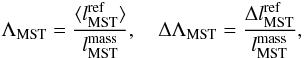 (1)provide a quantitative
measure of the degree of mass segregation: the larger ΛMST the more
concentrated are the massive stars compared to the reference sample; the associated
standard deviation ΔΛMST quantifies the significance of the result. To make
this method work and comparable also with observational data all calculations are carried
out in two dimensions, i.e. on a projection of the set of vertices.
(1)provide a quantitative
measure of the degree of mass segregation: the larger ΛMST the more
concentrated are the massive stars compared to the reference sample; the associated
standard deviation ΔΛMST quantifies the significance of the result. To make
this method work and comparable also with observational data all calculations are carried
out in two dimensions, i.e. on a projection of the set of vertices.
We have chosen the number of random reference samples, k, such that a
fraction p of the entire population of size N is
covered independent of the sample size n:
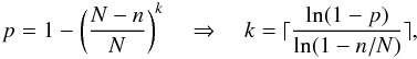 (2)where
⌈x⌉ denotes the ceiling function2 of x. The threshold has been set to
p = 0.99.
(2)where
⌈x⌉ denotes the ceiling function2 of x. The threshold has been set to
p = 0.99.
Our method
involves two crucial modifications of
that make it computationally much more effective and boost its sensitivity. First, unlike
Allison et al. (2009b) we do not calculate the
separations between all possible pairs of stars but determine the MST (in two dimensions)
in a three-step procedure: first we use a 2D Delaunay triangulation (from the software
package GEOMPACK: Joe 1991) to construct a useful
graph of stellar positions projected onto a plane, then we sort the edges of the triangles
in ascending order, and finally adapt Kruskal’s algorithm (Kruskal 1956) with an efficient union-find-algorithm to construct the MST.
A Delaunay triangulation has the very useful property that the MST construction (in any
dimension but for Euclidean distance) is its sub-graph (Preparata & Shamos 1985). The implementation of Joe (1991) involves a computational effort
 (3)similar to the edge
sorting by the quick-sort algorithm,
(3)similar to the edge
sorting by the quick-sort algorithm,
 (4)where
|E| is the number of edges and |V| the number of
vertices. With two algorithmic “tricks” in the union-find algorithm (“union by rank” and
“path compression”) we reduce its run-time to
(4)where
|E| is the number of edges and |V| the number of
vertices. With two algorithmic “tricks” in the union-find algorithm (“union by rank” and
“path compression”) we reduce its run-time to
 (5)where
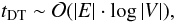
 (6)and thus rather constant
though in principle unlimited (Tarjan 1979). So the
total computational effort is dominated by the Delaunay triangulation and sorting of edges
and thus scales as
(6)and thus rather constant
though in principle unlimited (Tarjan 1979). So the
total computational effort is dominated by the Delaunay triangulation and sorting of edges
and thus scales as  (7)with
 .
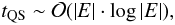
This is a significant improvement over the cost of the brute-force method,
.
This is a significant improvement over the cost of the brute-force method,
 .
.
Second, we do not use directly the sum of the edges
lMST as a measure yet their geometric
mean γMST,
![Mathematical equation: \begin{equation} \gmst = \bigg( \prod_{i=1}^n e_i \bigg)^{1/n} = \exp{ \left[ \frac{1}{n} \sum_{i=1}^n \ln{e_i} \right]}, \end{equation}](/articles/aa/full_html/2011/08/aa16902-11/aa16902-11-eq32.png) (8)and its
associated geometric standard deviation ΔγMST,
(8)and its
associated geometric standard deviation ΔγMST,
 (9)where
ei are the n MST edges.
Analogous to ΛMST, we obtain the new measure ΓMST via a proper
normalisation:
(9)where
ei are the n MST edges.
Analogous to ΛMST, we obtain the new measure ΓMST via a proper
normalisation:  (10)Note that the usage of a
geometric mean involves a multiplicative standard deviation ΔΓMST, i.e. the
upper and lower 1σ intervals are given by
ΓMST·(ΔΓMST)±1.
(10)Note that the usage of a
geometric mean involves a multiplicative standard deviation ΔΓMST, i.e. the
upper and lower 1σ intervals are given by
ΓMST·(ΔΓMST)±1.
The geometrical mean has two important properties that turn out to be very useful for our purpose of using the MST as a measure of mass segregation:
-
1.
The n-th root implicitly involves an intermediate-pass that damps contributions from extreme edge lengths very effectively (i.e. it gives a lower weight to very short or very long edges). Hence the mean edge length of a compact configuration of even few stars will not be affected much by an “outlier”. We demonstrate this property via a simple case of n−1 edges with length l = e0 and one very short “outlier” representing a tight binary with l = e1 = ϵe0, where ϵ ≪ 1 (e1 and ϵ could be also very large here in principle). Then the geometric mean would yield
 (11)In any practical
case (i.e. realistic star clusters models, observational data) the relevant binary
separation will be at most 3 orders of magnitude smaller than the mean separation of
single stars (or binary centre-of-mass)3.
So with ϵ = 10-3 we obtain even for a very small
sub-sample of n = 5 stars a mean edge length
⟨ l ⟩ ≈ 1/4e0.
This demonstrates the very effective damping of extreme values by the geometric
mean.
(11)In any practical
case (i.e. realistic star clusters models, observational data) the relevant binary
separation will be at most 3 orders of magnitude smaller than the mean separation of
single stars (or binary centre-of-mass)3.
So with ϵ = 10-3 we obtain even for a very small
sub-sample of n = 5 stars a mean edge length
⟨ l ⟩ ≈ 1/4e0.
This demonstrates the very effective damping of extreme values by the geometric
mean. -
2.
The product of edges has the valuable property that common edges in the two samples of massive and reference stars,
 and
and  ,
are cancelled out by normalisation, Eq. (10). So it is only the disjoint set of edge lengths that determines
ΓMST and hence the degree of mass segregation. Compared to
our scheme
is thus much more robust when applied to stellar systems with a high binary
fraction.
,
are cancelled out by normalisation, Eq. (10). So it is only the disjoint set of edge lengths that determines
ΓMST and hence the degree of mass segregation. Compared to
our scheme
is thus much more robust when applied to stellar systems with a high binary
fraction.
2.2. Primordial mass-segregation
A thorough test of our method
requires the generation of predefined mass segregated stellar systems. For this purpose we
found the method of Šubr et al. (2008) to be very
useful. The strength of the method is the generation of a well defined degree of mass
segregation that is controlled via one single parameter, S, and the
creation of dynamically consistent models by modelling local potentials and velocities in
a quasi-equilibrium state. The so-called index of mass segregation covers
the range S ∈ [0,1), where S = 0
corresponds to an entirely unsegregated state, while the upper limit
S = 1 marks the maximum possible segregation. In Fig. 1 we show two initially mass segregated models of
100 particles with S = 0.1 and S = 0.9 and their
corresponding MST, respectively.
 |
Fig. 1 Visualisation of the two-dimensional minimum spanning tree (MST) for numerical cluster models with different initial mass segregation parameters S (see Sect. 2.2). The solid blue lines (connecting the small black dots and large red dots) represent the MST of the entire population. The red dashed lines (connecting the large red dots) represent the MST of the ten most massive particles. Top: S = 0.1. Bottom: S = 0.9. |
In summary, the authors find that a mean inter-particle potential of the form
 (12)using ordered
subsets of stars,
(12)using ordered
subsets of stars, 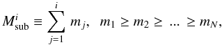 (13)provides one of
the simplest forms that characterise locally consistent mass segregation. This equation
provides a constraint on the distribution function from which one can construct a cluster
with the desired degree of mass segregation S by adding one-by-one the
individual stars from a mass-ordered set. The underlying distribution function
(13)provides one of
the simplest forms that characterise locally consistent mass segregation. This equation
provides a constraint on the distribution function from which one can construct a cluster
with the desired degree of mass segregation S by adding one-by-one the
individual stars from a mass-ordered set. The underlying distribution function
 (14)with
 (15)provides a good
estimate of the real distribution function of a Plummer sphere with mass segregation
index S.
(15)provides a good
estimate of the real distribution function of a Plummer sphere with mass segregation
index S.
The authors provide a numerical C-code plumix for generating the cluster according to the algorithm described in their paper on the AIfA web page: http://www.astro.uni-bonn.de
3. Results
In this section we provide examples showing the much better performance of
than .
However, we will also compare with the more traditional method
introduced in Sect. 1.
3.1. Special configurations
First, we will demonstrate the power of
for some simple setups of artificial mass segregation as shown in Fig. 2.
 |
Fig. 2 Three artificial configurations of massive stars with identical lMST in a model star cluster of 1 k members. Top: “cross”, Middle: “ring”, Bottom: “clump”. |
The idea to improve
and develop
was in fact motivated by the goal to find a measure that reflects the optical impression
of a lower or higher degree of mass segregation. The plots in Fig. 2 depict three different artificial configurations of the five most
massive stars in a star cluster of 1 k members, designated “cross”, “ring”, and “clump”,
from top to bottom. All these configurations are characterised by identical
lMST, i.e. according to
they represent the same degree of mass segregation. However, from an observer’s point of
view the cross appears to show a lower degree of mass segregation than the ring (i.e. the
latter appears more compact), while the clump would usually be interpreted as a highly
segregated system with a peculiar outlier.
Translated into a consistent algorithm we aim at measuring the compactness of a stellar
system by assigning a higher weight to the dominant configuration of stars and hence to
overcome the “degeneracy” of .
As already discussed in Sect. 2.1 this is mainly
achieved by damping the contribution from “outliers”, i.e. single edges with extreme
lengths ei compared to the median of all
edges, via the geometrical mean. Figure 3
demonstrates the effect of .
While by construction ΛMST (black dashed line) is identical for all three
configurations, ΓMST depends strongly on the degree of concentration of the
dominant sample of stars. Using the five most massive stars for the calculation of
ΓMST the highly concentrated “clump” shows a roughly two times higher degree
of mass segregation than the other two configurations. Also, it’s significance
(i.e. standard deviation in relation to the mean) is about 1.5 times higher than in the
case of ΛMST.
Note that though only the five most massive stars form a centrally concentrated configuration, i.e. are mass-segregated, one obtains a signature of mass segregation for a sample of up to 20 most massive stars. In particular, ΓMST of the ten most massive stars does even depend on the geometry of the configuration.
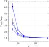 |
Fig. 3 Comparison of ΓMST (blue solid lines) and ΛMST (black dashed line) of three artificial configurations of massive stars in a model star cluster. From top to bottom, the solid lines with their symbols represent the artificial configuration “clump” (closed circles), “ring” (open circles), and “cross” (crosses). |
3.2. Initially mass-segregated clusters
Using the method of Šubr et al. (2008) to create initially mass-segregated star clusters (see Sect. 2.2) we have generated a set of low- to high-mass star clusters with 100, 1 k, 10 k, and 100 k stars, respectively. Their underlying mass function from Kroupa (2001) in the range 0.08−150 M⊙ results in an average stellar mass of ~0.6 M⊙. So our clusters span the mass range from 60 M⊙ to 60 k M⊙ which basically represents the entire observed cluster population in our Galaxy. All clusters have been set up with initial degrees of mass segregation S = {0.1,0.2,0.3,0.5,0.9} , each with ten configurations with different random seeds to reduce statistical uncertainties. However, in the following plots we show rescaled error bars that represent the statistical uncertainties of one single cluster.
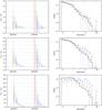 |
Fig. 4 Diagnostics of initially mass segregated star clusters with 1 k members following the prescription of Šubr et al. (2008). From top to bottom the degree of mass segregation, S, equals 0.1, 0.3, and 0.9 (see text for more details). On the left-hand side we compare ΓMST and ΛMST for the 5, 10, 20, 50, 100, 200, 500, 1000 most massive stars. The error bars and line thickness mark the 1σ, 2σ, and 3σ uncertainties. On the right-hand side we plot the corresponding mass function of the entire cluster population (solid black line), and the population within one (red tics), one-half (green crosses), and one-forth (blue dots) half-mass radius. The error bars mark the 1σ uncertainties. |
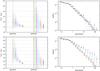 |
Fig. 5 Diagnostics of initially mass segregated star clusters with 10 k members following the prescription of Šubr et al. (2008). From top to bottom the degree of mass segregation, S, equals 0.1 and 0.3 (see text for more details). Details of the plots are given in the caption of Fig. 4. |
In Figs. 4 and 5 we show a selection of the most relevant results. On the left-hand side we compare ΓMST (“geometric”) and ΛMST (“arithmetic”) for the 5 (red), 10 (green), 20 (blue), 50 (magenta), 100 (cyan), 200 (brown), 500 (orange), and 1000 (black) most massive stars. The error bars and line thickness mark the 1σ, 2σ, and 3σ uncertainties. The horizontal dotted lines mark integer values, the horizontal dashed line represents the unsegregated state ΓMST = ΛMST = 1. Star clusters of intermediate masses ~1000 M⊙ are well observed in our local neighbourhood. These objects are represented by our simulations with 1 k particles. From Fig. 4 we find that our measure of mass segregation, ΓMST, detects a very low degree of mass segregation, S = 0.1, just above the 1σ-level, nearly independent of the number of most massive stars considered. The significance improves drastically for an intermediate degree of S = 0.3 to at least 3σ and even up to 4σ for the 20 to 100 most massive stars. Finally, for very strong mass segregation with S = 0.9 we obtain a very clear signature of more than 5σ for any number of (i.e. at least five) most massive stars.
These results are very much better than using ΛMST which never approaches a significance of 3σ and – in particular – for S = 0.3 provides only a very weak 1σ significance compared to 3−4σ in the case of ΓMST.
On the right-hand side we plot the corresponding mass functions for comparison with the
traditional method
to detect mass segregation. Here the mass function has been calculated in annuli with a
radius
r = {1/4 rh,1/2 rh,rh,rc} ,
where rh is the half-mass and rc
the total radius of the star cluster. It is clearly demonstrated that only very strong
mass segregation with S ≈ 0.9 becomes evident via this method. In this
case it is the mass range of stars around 10 M⊙ that
provides the strongest signature.
In contrast, our new measure ΓMST is much more effective. In particular, the 10 to 20 most massive stars of a 1 k star cluster usually provide the clearest signature of mass segregation.
Qualitatively, we find the same results for more massive clusters of 10 k stars in
Fig. 5:
provides the best measure of mass segregation by far. However, there are some important
quantitative differences. First, a much lower degree of mass segregation can be detected
for more massive clusters, e.g. for 10 k stars with S = 0.1 a
significance of 3σ is reached. Second, for a similar significance mass
segregation becomes most evident for a larger number of most massive stars, e.g. the
20 most massive stars for a 10 k system with S = 0.3 compared to the
10 most massive for a 1 k system with S = 0.9.
Both effects are in agreement with our expectations that in a more populous star cluster i) the same degree of mass segregation S will result in a higher relative concentration of the same number of most massive stars, i.e. ΓMST becomes larger; and ii) the absolute number of stars that show the same relative concentration is larger, i.e. ΔΓMST becomes lower.
The interplay of these two properties explains the existence and dependence of the local maximum of the significance of ΓMST: it peaks at the maximum ratio of ΓMST and ΔΓMST and thus increases for larger cluster masses and lower degrees of mass segregation towards larger numbers of most massive stars.
From our entire set of initially mass-segregated clusters we find that a sample size of 10 to 20 most massive stars generally provides the clearest signature of mass segregation.
Note that from Figs. 4 and 5 we conclude that using
the best estimate of mass segregation in star clusters from 1 k to 10 k members would be
for masses at ~10 M⊙ in an annulus of radius
r ≈ 1/4 rh.
3.3. Mass-segregation in the ONC
We recall that one of our goals was to develop a method that equally
well applies to data from simulations and observations and thus demonstrate the
excellent performance of
on observational data of the ~1 Myr old Orion nebula cluster (ONC) obtained by Hillenbrand (1997). The sample contains 929 stars with
mass estimates and so provides a robust test of the algorithm.
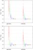 |
Fig. 6 Diagnostics of mass segregation in the young Orion nebula cluster (ONC) using observational data from Hillenbrand (1997). Top: ΓMST and ΛMST for the 5, 10, 20, 50, 100, 200, 500 most massive, and all 929 stars (left to right). Bottom: ΓMST and ΛMST for the 5, 6 to 10, 11 to 20, 21 to 50, 51 to 100, 101 to 200, 201 to 500, and 500 to 929 most massive stars (left to right). The error bars and line thickness mark the 1σ, 2σ, and 3σ uncertainties. |
The resulting plot of ΓMST for the 5, 10, 20, 50, 100, 200, 500 most massive, and all 929 stars in the upper part of Fig. 6 provides a clear signature of a significant concentration of the 20 most massive stars, much stronger than given by ΛMST. Interestingly, our calculation of ΛMST shows slightly stronger mass segregation than published by Allison et al. (2009a). Compared to the initially mass-segregated cluster models with 1 k particles presented in Fig. 4 the plot of ΓMST for the ONC shows a more complex distribution: there is a sharp drop between the 10 and 20 most massive stars. The significance of the first two data points (≳4σ) corresponds to the model with S = 0.9, the ≲3σ significance of the other resembles the much less segregated models with S ≤ 0.3.
In summary, i) mass segregation in the ONC at the current age ~1 Myr is much stronger than estimated before; and ii) it is clearly detectable not only for the five most massive stars yet for the 20 most massive objects.
However, the particular features of the ΓMST distribution require a more careful analysis. We do so by calculating ΓMST of disjoint particle groups, i.e. the most massive 5, 6 to 10, 11 to 20, etc. stars. The corresponding plot at the bottom of Fig. 6 shows that it is only the five most massive stars that are really strongly mass segregated (with a significance >4σ). Their configuration is so dominant that adding the next 15 most massive stars – which are not segregated – still shows a strong signature at the 3σ level, similar to the results in Sect. 3.1.
Hillenbrand (1997) argues that her sample of
combined photometric and spectroscopic data appears completely representative of the ONC,
showing in particular a uniform completeness with cluster radius. However, because
observational data are usually biased by incompleteness this issue is addressed in
Appendix A. We demonstrate that incompleteness
has only a moderate effect on
and provide a simple prescription for recovering the original signature of mass
segregation via the completeness function.
We conclude that all but the five most massive ONC stars do not show any signs of mass segregation. This result is in excellent agreement with Huff & Stahler (2006, Fig. 4. The five most massive stars’ extraordinary degree of mass segregation resembles their peculiar tight trapezium-like configuration (e.g. McCaughrean & Stauffer 1994; Hillenbrand & Hartmann 1998).
3.4. Dynamical evolution of mass-segregation
As a last application of our new method
we analyse again numerical data yet here we trace the dynamical evolution of a star
cluster model over time. The initial configuration is based on our ONC model as described
in previous publications (e.g. Olczak et al. 2010).
In short, it is a single star cluster with an isothermal initial density distribution, a
Maxwellian velocity distribution, the mass function of Kroupa (2001) in the range 0.08−150 M⊙, and an
initial size of 2.5 pc. Note that we use a spherically symmetric model with a smooth
density distribution without any substructure. However, in contrast to our basic
equilibrium model here our stellar system is initially collapsing, starting from a virial
ratio Q = 0.1. The simulations were carried out with Nbody64 (Aarseth 2003)
until a physical age of 5 Myr, corresponding to 13.5 N-body time units of
the cluster.
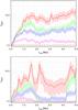 |
Fig. 7 Dynamical mass segregation in a star cluster with 1 k particles and cold initial conditions (Q = 0.1). The plots show the mean ΓMST (top) and ΛMST (bottom) of three simulations for the 5 (red solid line), 10 (green long-dashed line), 20 (blue short-dashed line), 50 (magenta dotted line), and 500 (orange dot-dashed line) most massive stars over time. The filled regions indicate 1σ uncertainties. |
In Fig. 7 we show the mean of three simulations of
the same model with different random seeds used to generate individual positions,
velocities, and masses. We plot ΓMST and ΛMST only for the 5, 10,
20, 50, and 500 most massive stars for reasons of visibility. The much better performance
of our improved method
compared to
is evident. Though both measures do show similar maximum degrees of mass segregation
ΛMST is subject to large variations over time. Only for the five most massive
stars does it show high significance over a longer period while for the 10 and 50 most
massive stars even values lower than one are quite common.
In contrast, ΓMST clearly increases over time with the steepest gradient within the first 2 Myr (or 5.5 N-body time units). It clearly separates the different mass groups, inversely correlated with the sample size. The much better robustness of ΓMST reflects again its very efficient damping of “outliers”.
We note that mass segregation in a collapsing, intermediate-size stellar cluster of 1 k stars can occur very quickly, i.e. within only a few crossing times. This finding demonstrates that rapid mass segregation (in terms of dynamical time scale) does not require substructure as has been recently investigated by Allison et al. (2009a). However, a detailed investigation of dynamical mass segregation in young star clusters will be presented in an upcoming publication.
4. Conclusion and discussion
We have developed a new method, ,
to measure mass segregation by significantly improving a previous approach of Allison et al. (2009a) based on the minimum spanning tree
(MST), here referred to as .
Their method uses the normalised length of the MST of a given sample of stars,
ΛMST, as a measure of compactness.
Compared to “classical” measures of mass segregation such as the slope of the
(differential) mass function in different annuli around the cluster centre (see Sect. 1), ΛMST overcomes several substantial
weaknesses. Our new method
inherits all the advantages provided by :
-
independence of cluster geometry,
-
no requirement of cluster centre,
-
no requirement of quantitative measure of masses,
-
one-parametric unique measure of mass segregation,
and adds three significant improvements:
-
nearly linear computational efficiency,
-
robustness against peculiar configurations, and
-
high sensitivity.
This gain is based on two boosting ingredients:
-
1.
the implementation of an efficient
 )
algorithm for thecalculation of the MST, and
)
algorithm for thecalculation of the MST, and -
2.
the calculation of the geometrical mean of the connecting edges, ΓMST, instead of just their sum, ΛMST.
The high performance is achieved by construction of a graph via 2D Delaunay triangulation (from the software package GEOMPACK: Joe 1991), quick sorting of its edges, and an efficient numerical implementation of Kruskal’s algorithm (Kruskal 1956). The advantage of the geometrical mean is that it damps the contribution of “outliers” very efficiently and thus traces the concentration of the dominant stars of a configuration.
We have demonstrated the advantage of
compared to other known and frequently used methods via various examples, both for numerical
and observational data.
-
1.
In general, using only the ten to twenty most massive stars ΓMSTprovides a robust and sensitive measure of mass segregation forthe entire population of star clusters in our Galaxy.
-
2.
In particular, very low degrees of mass segregation can be detected in massive clusters like NGC 3603 that consist of 10 k or more stars.
-
3.
We have also confirmed the very strong mass segregation of the five most massive stars in the ONC as reported by Huff & Stahler (2006).
-
4.
Incompleteness of observational data has only a moderate effect on
and corrections can be implemented easily similar to methods
like .
However, we also stress three important aspects that have to be considered for a careful
investigation of mass segregation via :
-
1.
Our conclusion that the 10 to 20 most massive stars generallyprovide the most sensitive measure of mass segregation has beenderived from model clusters with smooth mass segregation overthe entire sample. We caution that this is not to be expected if onlyspecific subsamples are affected by mass segregation(as shown for the five most massive stars of theONC in Sect. 3.3); this is of particular concern forstudies of primordial mass segregation. We thus generallyrecommend to use both the cumulative and the differentialanalysis of a set of mass groups to investigate mass segregation in(young) star clusters.
-
2.
The signature of a small sub-sample can be strong enough to bias ΓMST of a larger parent sample. To avoid wrong conclusions one should also calculate ΓMST of disjoint samples, e.g. of the 5, 6 to 10, 11 to 20 etc. most massive stars.
-
3.
The value of ΓMST of a sub-sample is independent of its location with respect to the entire sample. It only reflects the compactness of this sub-sample, not its concentration towards some centre of the entire sample. So a large ΓMST does not necessarily mean that the corresponding sub-sample is mass-segregated. Thus, in practice, in particular when dealing with observational data, the determination of some centre of the sample as reference point is still required. However, the value of ΓMST remains independent of the reference point and so its advantage compared to other methods.
Our improved method
will be vital for future studies of mass segregation in stellar systems. Its robustness and
sensitivity is ideal for tracing lower degrees and more complex types of mass segregation
than before. This is of particular interest for the earliest stages of star formation that
seem to form protoclusters of complex structure (e.g. Teixeira et al. 2006). Furthermore, it will also help to investigate the question
whether mass segregation is observed at all in young star clusters (e.g. Ascenso et al. 2009). Finally, our method can be used in
general for precise structure analysis of any type of stellar system from planetary debris
disks to galaxy clusters.
As a first application of
to numerical simulations we have demonstrated that mass segregation in young star clusters
can occur very quickly under dynamically cold initial conditions. Indeed we do expect young
stellar systems to form under such conditions as a result of the gravitational collapse of
their parent molecular cloud. Whether collapse still occurs in largely evolved young
clusters like the ONC – the scenario corresponding to our simulation – is still unknown yet
became favoured recently (e.g. Jones & Walker
1988; Kroupa 2000; Scally et al. 2005; Fűrész et al.
2008; Proszkow et al. 2009; Tobin et al. 2009). However, at least some fraction of
the oldest stars must have formed during global collapse. Hence rapid mass segregation
affects the structure of star forming regions at the earliest stages and could thus explain
the observed mass segregation of the most massive stars in the ONC.
We will investigate this and other aspects of dynamical mass segregation in young star clusters under various conditions in an upcoming publication.
A variant of the MST method has been presented just recently by Yu et al. (2011) at the time of submission of our publication.
The ceiling function ⌈x⌉ gives the lowest integer larger than or equal to x.
This estimate is based on the following reference values: the mean stellar separation in the Orion nebula cluster is about 2.5 pc/40001/3 ≈ 0.15 pc ≈ 30 000 AU; the HST has a resolution of ~50 AU at an assumed distance of 400 pc (Menten et al. 2007; Jeffries 2007; Kraus et al. 2009). Thus, binaries with separations ≲10-3 would remain unresolved.
Note that we have used the GPU enabled version of Nbody6 available at http://www.ast.cam.ac.uk/research/nbody
Acknowledgments
C.O. and R.S. acknowledge support by NAOC CAS through the Silk Road Project, and by Global Networks and Mobility Program of the University of Heidelberg (ZUK 49/1 TP14.8 Spurzem). C.O. appreciates funding by the German Research Foundation (DFG), grant OL 350/1-1. R.S. is funded by the Chinese Academy of Sciences Visiting Professorship for Senior International Scientists, Grant Number 2009S1-5. We have partly used the special supercomputers at the Center of Information and Computing at National Astronomical Observatories, Chinese Academy of Sciences, funded by Ministry of Finance of Peoples Republic of China under the grant ZDY Z20082. We thank S. Aarseth for providing the highly sophisticated N-body code Nbody6 (and its GPU extension) and greatly appreciate his support.
References
- Aarseth, S. 2003, Gravitational N-body Simulations (Cambridge: Cambridge University Press), 430 [Google Scholar]
- Allison, R. J., Goodwin, S. P., Parker, R. J., et al. 2009a, ApJ, 700, L99 [NASA ADS] [CrossRef] [Google Scholar]
- Allison, R. J., Goodwin, S. P., Parker, R. J., et al. 2009b, MNRAS, 395, 1449 [Google Scholar]
- Ascenso, J., Alves, J., & Lago, M. T. V. T. 2009, A&A, 495, 147 [NASA ADS] [CrossRef] [EDP Sciences] [Google Scholar]
- Bolte, M. 1989, ApJ, 341, 168 [NASA ADS] [CrossRef] [Google Scholar]
- Cartwright, A., & Whitworth, A. P. 2004, MNRAS, 348, 589 [NASA ADS] [CrossRef] [Google Scholar]
- Evans, N. J., Dunham, M. M., Jørgensen, J. K., et al. 2009, ApJS, 181, 321 [NASA ADS] [CrossRef] [Google Scholar]
- Farouki, R. T., Hoffman, G. L., & Salpeter, E. E. 1983, ApJ, 271, 11 [NASA ADS] [CrossRef] [Google Scholar]
- Fűrész, G., Hartmann, L. W., Megeath, S. T., Szentgyorgyi, A. H., & Hamden, E. T. 2008, ApJ, 676, 1109 [NASA ADS] [CrossRef] [Google Scholar]
- Gower, J. C., & Ross, G. J. S. 1969, J. Roy. Stat. Soc. Ser. C (Appl. Stat.), 18, 54 [Google Scholar]
- Hillenbrand, L. A. 1997, AJ, 113, 1733 [NASA ADS] [CrossRef] [Google Scholar]
- Hillenbrand, L. A., & Hartmann, L. W. 1998, ApJ, 492, 540 [NASA ADS] [CrossRef] [Google Scholar]
- Huff, E. M., & Stahler, S. W. 2006, ApJ, 644, 355 [NASA ADS] [CrossRef] [Google Scholar]
- Jeffries, R. D. 2007, MNRAS, 376, 1109 [NASA ADS] [CrossRef] [Google Scholar]
- Joe, B. 1991, Advances in Engineering Software, 13, 325 [Google Scholar]
- Jones, B. F., & Walker, M. F. 1988, AJ, 95, 1755 [NASA ADS] [CrossRef] [Google Scholar]
- Khalisi, E., Amaro-Seoane, P., & Spurzem, R. 2007, MNRAS, 374, 703 [NASA ADS] [CrossRef] [Google Scholar]
- Kraus, S., Weigelt, G., Balega, Y. Y., et al. 2009, A&A, 497, 195 [NASA ADS] [CrossRef] [EDP Sciences] [Google Scholar]
- Kroupa, P. 2000, New Astron., 4, 615 [NASA ADS] [CrossRef] [Google Scholar]
- Kroupa, P. 2001, MNRAS, 322, 231 [NASA ADS] [CrossRef] [Google Scholar]
- Kruskal, J. B., J. 1956, Proc. Am. Math. Soc., 7, 48 [Google Scholar]
- Lada, C. J., & Lada, E. A. 2003, ARA&A, 41, 57 [NASA ADS] [CrossRef] [Google Scholar]
- McCaughrean, M. J., & Stauffer, J. R. 1994, AJ, 108, 1382 [NASA ADS] [CrossRef] [Google Scholar]
- Menten, K. M., Reid, M. J., Forbrich, J., & Brunthaler, A. 2007, A&A, 474, 515 [NASA ADS] [CrossRef] [EDP Sciences] [Google Scholar]
- Olczak, C., Pfalzner, S., & Eckart, A. 2010, A&A, 509, A26 [Google Scholar]
- Pandey, A. K., Mahra, H. S., & Sagar, R. 1992, Bull. Astron. Soc. India, 20, 287 [Google Scholar]
- Preparata, F. P., & Shamos, M. I. 1985, Computational geometry, an introduction (New York Inc.: Springer) [Google Scholar]
- Proszkow, E.-M., Adams, F. C., Hartmann, L. W., & Tobin, J. J. 2009, ApJ, 697, 1020 [NASA ADS] [CrossRef] [Google Scholar]
- Richer, H. B., Fahlman, G. G., & Vandenberg, D. A. 1988, ApJ, 329, 187 [NASA ADS] [CrossRef] [Google Scholar]
- Scally, A., Clarke, C., & McCaughrean, M. J. 2005, MNRAS, 358, 742 [NASA ADS] [CrossRef] [Google Scholar]
- Schmeja, S., & Klessen, R. S. 2006, A&A, 449, 151 [NASA ADS] [CrossRef] [EDP Sciences] [Google Scholar]
- Spitzer, L. J. 1969, ApJ, 158, L139 [NASA ADS] [CrossRef] [Google Scholar]
- Spurzem, R., & Takahashi, K. 1995, MNRAS, 272, 772 [NASA ADS] [Google Scholar]
- Stolte, A., Brandner, W., Brandl, B., & Zinnecker, H. 2006, AJ, 132, 253 [NASA ADS] [CrossRef] [Google Scholar]
- Tarjan, R. E. 1979, J. ACM, 26, 690 [CrossRef] [Google Scholar]
- Teixeira, P. S., Lada, C. J., Young, E. T., et al. 2006, ApJ, 636, L45 [NASA ADS] [CrossRef] [Google Scholar]
- Tobin, J. J., Hartmann, L., Furesz, G., Mateo, M., & Megeath, S. T. 2009, ApJ, 697, 1103 [NASA ADS] [CrossRef] [Google Scholar]
- Šubr, L., Kroupa, P., & Baumgardt, H. 2008, MNRAS, 385, 1673 [NASA ADS] [CrossRef] [Google Scholar]
- Yu, J., de Grijs, R., & Chen, L. 2011, ApJ, 732, 16 [NASA ADS] [CrossRef] [Google Scholar]
Appendix A: Data incompleteness and ΓMST
We provide an example on how incompleteness of observational data affects ΓMST and present a simple prescription for recovering the original signature of mass segregation via the corresponding completeness function.
Here we use again the original sample of 929 stars in the ONC from Hillenbrand (1997) to generate a reduced sample via convolution with an
artificial completeness function with radial and mass dependence of the form ![Mathematical equation: \appendix \setcounter{section}{1} \begin{eqnarray} c( r, r_{{\rm u}}, p, a_{{\rm l}}, a_{{\rm u}}, m, m_{{\rm l}}, m_{{\rm u}}, b_{{\rm l}}, b_{{\rm u}} ) &&= \nonumber\\ \label{eq:completeness}&& 1 - \exp \left\{ {\cal{R}}( r, r_{{\rm u}}, p, a_{{\rm l}}, a_{{\rm u}} ) \left[ {\cal{M}}(m, m_{{\rm l}}, m_{{\rm u}}) \right]^{{\cal{R}}(r, r_{{\rm u}}, p, b_{{\rm l}}, b_{{\rm u}} ) } \right\}, \end{eqnarray}](/articles/aa/full_html/2011/08/aa16902-11/aa16902-11-eq94.png) (A.1)where
(A.1)where
 \arraycolsep1.75ptand
the indices l and u denote lower and upper values, respectively.
\arraycolsep1.75ptand
the indices l and u denote lower and upper values, respectively.
The parameters used to simulate loss of data due to observational incompleteness are presented in Table A.1. The corresponding plot in Fig. A.1 shows the completeness as a function of stellar mass in dependence of radial position in the cluster. From right to left the graphs represent increasing radii in steps of 0.25 pc from the centre to 2.5 pc, the outer boundary of the ONC. The solid (red), dashed (blue), and dotted (black) lines are grouped in steps of 1 pc, respectively.
The functional form has been adopted such that it resembles observational incompleteness due to crowding in the dense and bright cluster centre and due to individual extinction over the entire cluster. It is expected that stars with masses ≳10 M⊙ are too bright to be missed while low-mass objects close to the cluster centre with it’s four luminous Trapezium stars remain mostly undetected.
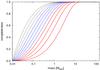 |
Fig. A.1 Model of completeness as a function of stellar mass and radial position in the ONC according to Eq. (A.1) and using the parameters from Table A.1. From right to left the graphs represent increasing radii in steps of 0.25 pc from the centre to 2.5 pc, the outer boundary of the ONC. The solid (red), dashed (blue), and dotted (black) lines are grouped in steps of 1 pc, respectively. |
To reconstruct a larger unbiased sample from the incomplete sample we have used the inverse completeness function in the following simple prescription:
-
1.
Go to the next object i in the incomplete sample.
-
2.
Calculate its completeness ci using its radial position ri and mass mi.
-
3.
If ci > cmin:
-
(a)
calculate the missing number of objects ni = 1/ci−1 with ri and mi,
-
(b)
generate for each additional object j its
-
i.
mass mj = mi(1 + λ), λ ∈ [−0.05,0.05] a random number, and
-
ii.
radial position rj = ri(1 + η), η ∈ [−0.1,0.1] a random number.
-
i.
-
(a)
We compare ΓMST of the three samples – original, incomplete, and reconstructed – in Fig. A.2. The left-hand side shows ΓMST of the 5, 10, 20, 50, 100, 200, 500 most massive, and all stars, i.e. cumulative mass groups; the right-hand side shows ΓMST of the 5, 6 to 10, 11 to 20, 21 to 50, 51 to 100, 101 to 200, 201 to 500, and 500 to all most massive stars, i.e. differential mass groups. The top plot refers to the original sample of 929 ONC stars: it is the same data as on the left-hand side of Fig. 6. Below we plot ΓMST of the incomplete sample that has been artificially reduced to 485 stars via Eq. (A.1). This removal of nearly half the cluster population – preferentially low-mass stars in the cluster centre – has a marginal effect on ΓMST: only for the five and ten most massive stars a significant difference is observed. However, the differential plot reveals again a dominant contribution from the five most massive stars, ΓMST of the 6−10 most massive remains nearly unchanged.
The bottom plot contains data of additional 345 cloned objects and so 830 stars in total – about 10% less than the original sample. The reconstruction procedure seems to work fairly well: ΓMST of the five and ten most massive stars is indistinguishable from its original values. However, the next intervals up to the 200 most massive stars all show slightly lower degrees of mass segregation than originally. The reason is that the sample of even less massive stars (200−500 and 500−830 most massive stars) is marginally mass segregated (i.e. ΓMST > 1 unlike in the original sample): these low-mass stars that make up the main part of the random reference sample were cloned preferentially closer to the cluster centre which reduced ΓMST of the more massive stars.
However, considering the reconstruction of up to 80% individual incompleteness and nearly half of the entire incomplete sample, the result is very promising: the strong conclusion for the original sample that the five most massive stars in the ONC are highly mass segregated while all other stars do not show any signature of mass segregation remains unchanged for the reconstructed sample.
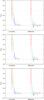 |
Fig. A.2 Diagnostics of mass segregation for three sets of observational data of the young Orion nebula cluster (ONC). The left-hand side shows from left to right ΓMST of the 5, 10, 20, 50, 100, 200, 500 most massive, and all stars, i.e. cumulative mass groups; the right-hand side shows from left to right ΓMST of the 5, 6 to 10, 11 to 20, 21 to 50, 51 to 100, 101 to 200, 201 to 500, and 500 to all most massive stars, i.e. differential mass groups. The error bars and line thickness mark the 1σ, 2σ, and 3σ uncertainties. Top: original set of 929 stars observed by Hillenbrand (1997). Middle: incomplete sample. Bottom: reconstructed sample. |
All Tables
All Figures
|
Fig. 1 Visualisation of the two-dimensional minimum spanning tree (MST) for numerical cluster models with different initial mass segregation parameters S (see Sect. 2.2). The solid blue lines (connecting the small black dots and large red dots) represent the MST of the entire population. The red dashed lines (connecting the large red dots) represent the MST of the ten most massive particles. Top: S = 0.1. Bottom: S = 0.9. |
| In the text | |
|
Fig. 2 Three artificial configurations of massive stars with identical lMST in a model star cluster of 1 k members. Top: “cross”, Middle: “ring”, Bottom: “clump”. |
| In the text | |
|
Fig. 3 Comparison of ΓMST (blue solid lines) and ΛMST (black dashed line) of three artificial configurations of massive stars in a model star cluster. From top to bottom, the solid lines with their symbols represent the artificial configuration “clump” (closed circles), “ring” (open circles), and “cross” (crosses). |
| In the text | |
|
Fig. 4 Diagnostics of initially mass segregated star clusters with 1 k members following the prescription of Šubr et al. (2008). From top to bottom the degree of mass segregation, S, equals 0.1, 0.3, and 0.9 (see text for more details). On the left-hand side we compare ΓMST and ΛMST for the 5, 10, 20, 50, 100, 200, 500, 1000 most massive stars. The error bars and line thickness mark the 1σ, 2σ, and 3σ uncertainties. On the right-hand side we plot the corresponding mass function of the entire cluster population (solid black line), and the population within one (red tics), one-half (green crosses), and one-forth (blue dots) half-mass radius. The error bars mark the 1σ uncertainties. |
| In the text | |
|
Fig. 5 Diagnostics of initially mass segregated star clusters with 10 k members following the prescription of Šubr et al. (2008). From top to bottom the degree of mass segregation, S, equals 0.1 and 0.3 (see text for more details). Details of the plots are given in the caption of Fig. 4. |
| In the text | |
|
Fig. 6 Diagnostics of mass segregation in the young Orion nebula cluster (ONC) using observational data from Hillenbrand (1997). Top: ΓMST and ΛMST for the 5, 10, 20, 50, 100, 200, 500 most massive, and all 929 stars (left to right). Bottom: ΓMST and ΛMST for the 5, 6 to 10, 11 to 20, 21 to 50, 51 to 100, 101 to 200, 201 to 500, and 500 to 929 most massive stars (left to right). The error bars and line thickness mark the 1σ, 2σ, and 3σ uncertainties. |
| In the text | |
|
Fig. 7 Dynamical mass segregation in a star cluster with 1 k particles and cold initial conditions (Q = 0.1). The plots show the mean ΓMST (top) and ΛMST (bottom) of three simulations for the 5 (red solid line), 10 (green long-dashed line), 20 (blue short-dashed line), 50 (magenta dotted line), and 500 (orange dot-dashed line) most massive stars over time. The filled regions indicate 1σ uncertainties. |
| In the text | |
|
Fig. A.1 Model of completeness as a function of stellar mass and radial position in the ONC according to Eq. (A.1) and using the parameters from Table A.1. From right to left the graphs represent increasing radii in steps of 0.25 pc from the centre to 2.5 pc, the outer boundary of the ONC. The solid (red), dashed (blue), and dotted (black) lines are grouped in steps of 1 pc, respectively. |
| In the text | |
|
Fig. A.2 Diagnostics of mass segregation for three sets of observational data of the young Orion nebula cluster (ONC). The left-hand side shows from left to right ΓMST of the 5, 10, 20, 50, 100, 200, 500 most massive, and all stars, i.e. cumulative mass groups; the right-hand side shows from left to right ΓMST of the 5, 6 to 10, 11 to 20, 21 to 50, 51 to 100, 101 to 200, 201 to 500, and 500 to all most massive stars, i.e. differential mass groups. The error bars and line thickness mark the 1σ, 2σ, and 3σ uncertainties. Top: original set of 929 stars observed by Hillenbrand (1997). Middle: incomplete sample. Bottom: reconstructed sample. |
| In the text | |
Current usage metrics show cumulative count of Article Views (full-text article views including HTML views, PDF and ePub downloads, according to the available data) and Abstracts Views on Vision4Press platform.
Data correspond to usage on the plateform after 2015. The current usage metrics is available 48-96 hours after online publication and is updated daily on week days.
Initial download of the metrics may take a while.