| Issue |
A&A
Volume 695, March 2025
|
|
|---|---|---|
| Article Number | A188 | |
| Number of page(s) | 9 | |
| Section | Galactic structure, stellar clusters and populations | |
| DOI | https://doi.org/10.1051/0004-6361/202451785 | |
| Published online | 18 March 2025 | |
Massive star cluster formation
III. Early mass segregation during cluster assembly
1
Universität Heidelberg, Zentrum für Astronomie, Institut für Theoretische Astrophysik,
Heidelberg,
Germany
2
Department of Astrophysics, American Museum of Natural History,
New York,
NY,
USA
3
Universität Heidelberg, Interdisziplinäres Zentrum für Wissenschaftliches Rechnen,
Heidelberg,
Germany
4
Harvard-Smithsonian Center for Astrophysics,
Cambridge,
MA,
USA
5
Radcliffe Institute for Advanced Studies at Harvard University,
Cambridge,
MA,
USA
6
Sterrewacht Leiden, Leiden University,
Leiden,
The Netherlands
7
Department of Physics and Astronomy, Rutgers University,
Piscataway,
NJ,
USA
8
Department of Physics and Astronomy, McMaster University,
Hamilton,
ON,
Canada
9
Department of Physics, Drexel University,
Philadelphia,
PA,
USA
★ Corresponding author; This email address is being protected from spambots. You need JavaScript enabled to view it.
Received:
3
August
2024
Accepted:
18
February
2025
Abstract
Mass segregation is seen in many star clusters, but whether massive stars form in the center of a cluster or migrate there dynamically is still debated. N-body simulations show that early dynamical mass segregation is possible when sub-clusters merge to form a dense core with a small crossing time. However, the effect of gas dynamics on both the formation and dynamics of the stars could inhibit the formation of the dense core. We aim to study the dynamical mass segregation of star cluster models that include gas dynamics and selfconsistently form stars from the dense substructure in the gas. Our models use the TORCH framework, which is based on AMUSE and includes stellar and magnetized gas dynamics, as well as stellar evolution and feedback from radiation, stellar winds, and supernovae. Our models consist of three star clusters forming from initial turbulent spherical clouds of mass 104, 105, 106 M⊙ and radius 11.7 pc that have final stellar masses of 3.6 × 10³ M⊙, 6.5 × 10⁴ M⊙, and 8.9 × 10⁵ M⊙, respectively. There is no primordial mass segregation in the model by construction. All three clusters become dynamically mass segregated at early times via collapse confirming that this mechanism occurs within sub-clusters forming directly out of the dense substructure in the gas. The dynamics of the embedded gas and stellar feedback do not inhibit the collapse of the cluster. We find that each model cluster becomes mass segregated within 2 Myr of the onset of star formation, reaching the levels observed in young clusters in the Milky Way. However, we note that the exact values are highly time-variable during these early phases of evolution. Massive stars that segregate to the center during core collapse are likely to be dynamically ejected, a process that can decrease the overall level of mass segregation again.
Key words: stars: formation / ISM: clouds / galaxies: star clusters: general
Fellow of the International Max Planck Research School for Astronomy and Cosmic Physics at the University of Heidelberg.
NSF Astronomy & Astrophysics Postdoctoral Fellow.
© The Authors 2025
 Open Access article, published by EDP Sciences, under the terms of the Creative Commons Attribution License (https://creativecommons.org/licenses/by/4.0), which permits unrestricted use, distribution, and reproduction in any medium, provided the original work is properly cited.
This article is published in open access under the Subscribe to Open model. This email address is being protected from spambots. You need JavaScript enabled to view it. to support open access publication.
1 Introduction
Most stars form from giant molecular clouds (GMCs) in groups of tens to millions of stars called star clusters (see, e.g., Lada & Lada 2003; Portegies Zwart et al. 2010; Krause et al. 2020). Models suggest that star clusters form from the global hierarchical collapse of GMCs (Vázquez-Semadeni et al. 2017; Grudić et al. 2018). As the GMC undergoes gravoturbulent collapse (Larson 1981), fragmentation leads to the formation of dense star-forming clumps (Mac Low & Klessen 2004; McKee & Ostriker 2007; Klessen & Glover 2016) called sub-clusters. These sub-clusters eventually merge if they are gravitationally bound, collapsing into a single star cluster.
Many star clusters exhibit signs of mass segregation where the massive stars are concentrated in the center of the cluster (Hillenbrand & Hartmann 1998). This can happen dynamically when massive stars migrate to the center via two-body interactions (Spitzer 1969), or it can occur primordially when massive stars are preferentially formed in the center where the gas density is highest (e.g., Klessen & Burkert 2000; McKee & Tan 2003). Determining whether and when one of these modes of mass segregation dominates is essential for understanding the formation of stars and assembly of star clusters; whether star formation is spatially distributed randomly or according to mass presents two entirely different pictures of star formation.
If a young star cluster is observed to be mass segregated earlier than expected given the cluster’s crossing time, this would necessitate primordial mass segregation. However, N-body models presented in Allison et al. (2009b) suggest a mechanism that allows for clusters to become dynamically segregated at much earlier times. They suggest that the collapse1 of the star cluster – when sub-clusters merge and create a short-lived dense core – facilitates efficient and early dynamical mass segregation. However, it is unclear whether sub-clusters forming self-consistently from a collapsing GMC would still merge in a way that creates this dense core. Furthermore, including gas dynamics could also inhibit the collapse of the cluster’s central region.
We examine the mass segregation in three star cluster models, first presented in Polak et al. (2024, hereafter Paper I). These simulations resolve individual stars down to 4 M⊙ forming from an initially turbulent spherical cloud of gas. By construction, the stars in our model are not primordially mass segregated. Thus we specifically study the timescale on which dynamical mass segregation occurs. We find that this process becomes important earlier than proposed by Allison et al. (2009b), as transient periods of mass segregation occur even before the global collapse of the cluster. We confirm that sub-clusters forming self-consistently from the cloud’s substructure do form the dense cores needed for early dynamical segregation, and the embedding gas does not inhibit the collapse necessary for this mechanism.
We briefly introduce our three star cluster models in Section 2, and in Section 3 we present the progression of mass segregation over each cluster’s lifetime. In Section 4, we examine the expected timescales for dynamical mass segregation and compare the degree of mass segregation in our clusters to observations in order to address whether primordial mass segregation is necessary to explain the mass segregation observed in young Galactic clusters. We conclude in Section 5.
2 Methods
We perform simulations of star clusters forming from turbulent spherical clouds of gas with TORCH2 (Wall et al. 2019, 2020). The TORCH framework couples the magnetohydrodynamics code FLASH (Fryxell et al. 2000), the N-body code PETAR (Wang et al. 2020), and the stellar evolution code SEBA (Portegies Zwart & Verbunt 1996) via the Astrophysical MUltipurpose Software Environment (AMUSE; Portegies Zwart et al. 2009; Portegies Zwart et al. 2013; Pelupessy et al. 2013; Portegies Zwart & McMillan 2018). Together, these three codes handle the magnetized gas dynamics, individual star formation via sink particles, stellar dynamics, stellar evolution, and stellar feedback in the form of radiation, winds, and supernovae (SNe). We provide a brief review of the numerical methods used by TORCH in this section; for more details, see Paper I, Wall et al. (2019), and Wall et al. (2020).
FLASH is an adaptive mesh refinement grid code. We refined the grid on temperature and pressure gradients as well as the Jeans length λJ = (π cs2/[G ρ])1/2 of the gas. We used the HLLD Riemann solver (Miyoshi & Kusano 2005) with third-order piecewise parabolic method reconstruction (Colella & Woodward 1984). A multigrid Poisson gravity solver (Ricker 2008) calculates the gas self-gravity, and a leapfrog gravity-bridge (Fujii et al. 2007; Wall et al. 2019; Portegies Zwart et al. 2020) calculates the gravitational interaction between the star particles and gas.
Sub-grid star formation in TORCH is modeled with sink particles (Federrath et al. 2010). Briefly described, when the local gas density exceeds the Jeans density at the maximum level of refinement (ρsink), a sink particle is formed to collect the dense, star-forming gas which would otherwise be unresolved. Physically, sink particles represent star-forming cores of dense gas.
Following the Truelove et al. (1997) criterion to avoid artificial fragmentation, we set λJ = 5 Δ x = 2 rsink. Upon formation, the mass of the gas denser than ρsink and within the sink’s accretion radius rsink is removed from the domain and added to the sink particle’s mass. Sink particles have a list of stellar masses randomly sampled from the Kroupa (2002) initial mass function (IMF), and the sinks form the next star on the list as soon as they accrete the required amount of mass. Primordial mass segregation does not occur globally in our models because every sink has a high enough star formation rate that they all fully sample the IMF.
The accelerations of sink particles have contributions from other sinks, gas, and stars. The gravitational acceleration from other sinks is calculated by direct summation. Star particle gravity is combined with the gas by a cloud-in-cell mapping of stellar masses onto the grid. The gravitational acceleration from the gas and stars is then calculated using the potential returned by the multigrid Poisson solver. The acceleration on the gas due to sinks is calculated by a direct summation using the distance from the sink to each gas cell center. The sink particle masses are also mapped onto the gas cells and used to calculate the acceleration of sinks on star particles. Sink particles are allowed to merge in TORCH, but with ≲ 20 sinks in our models this rarely occurs. The time between accretion and star formation is less than a timestep for the majority of these simulations, so the effect of sink dynamics on star formation is negligible.
Stars are placed in a uniform random distribution within the sink’s accretion radius, thereby suppressing any primordial mass segregation within the sink volume. The star’s velocity is set by adding the sink’s velocity to a velocity component with the magnitude sampled from a Gaussian distribution with variance σ = cs and with the direction sampled isotropically. The local sound speed cs is calculated by averaging the sound speed of cold gas (≤ 100 K) within 2 rsink. The sink does not form stars if there is no cold gas in the sink’s vicinity.
The modes of stellar feedback implemented in TORCH are radiation, winds, and SNe (Wall et al. 2020). The stellar evolution code SEBA evolves star particles from the zero-age main sequence until their stellar death, and provides the stellar feedback properties for the routines in FLASH. Two frequency groups of radiation, both ionizing and non-ionizing ultraviolet, are propagated via the Fervent ray-tracing module (Baczynski et al. 2015).
We use the M4, M5, and M6 simulations introduced in Paper I which have initial cloud masses 104, 105, and 106 M⊙, respectively. The varying and shared simulation properties of the initial clouds are listed in Table 1. We aimed to keep the clouds as similar as possible to investigate the isolated effect of cloud mass on star cluster properties.
The radius of all three clouds is Rcloud = 11.7 pc, so the density of the clouds increases with mass. We set the initial density profile of the cloud to be a Gaussian (Bate et al. 1995; Goodwin et al. 2004) where ρedge/ρc = 1/3. Our boundary conditions allow gas to flow into or out of the domain to prevent vacuums forming at the edge (see Paper I for details). The initial turbulence of the gas is set by a Kolmogorov (1941) velocity spectrum using the same random seed for each simulation. With the same cloud radius, this results in the same morphology and spatial distribution of forming dense cores and stars facilitating comparisons between the three clouds. We set the initial magnetic field B = Bz ẑ to be uniform in the z direction and decrease radially with the mid-plane density ρ(x, y, z = 0) in the x–y plane: Bz(x, y) = B0, z exp [−(x2 + y2) ln (3)/Rcloud2] where the values of B0, z are listed in Table 1.
We made a few modifications to standard TORCH in order to feasibly accommodate the large number of stars formed in the 105 M⊙ and 106 M⊙ clouds. Paper I provides an in-depth description of the modifications and an analysis of their effect. The relevant alteration for this paper is that we agglomerate low-mass stars below Magg = 4 M⊙ into single star particles with summed masses > 4 M⊙, which reduces the number of star particles on the grid by ≈ 90%. We agglomerate the star particles that are < 4 M⊙ in the order they are sampled until their combined mass is ≥ 4 M⊙. The mass of agglomerated star particles can lie between 4−8 M⊙3, but on average they are ∼ 4.5 M⊙. Without agglomeration, the N-body code would have to compute the dynamics of > 106 stars in the case of M6.
Simulation parameters.
3 Results
We quantified the degree of mass segregation in a star cluster using a minimum spanning tree (MST) method as described by Allison et al. (2009a). The basic idea is to use the total edge length of the MST formed by a group of stars to quantify their proximity to each other. This method compares the total edge length (ℓmassive) of the MST made by the NMST most massive stars in a cluster to the average total edge length (ℓrand) of nsample MSTs formed by the same number of randomly selected stars.
This gives a simple and comprehensive way of comparing the proximity of massive stars to that of all the stars in the cluster. This quantifies the mass segregation as a mass segregation ratio Λ, calculated by
 (1)
(1)
where σrand is the standard deviation of the ℓrand values. Mass segregation is present when Λ > 1. We use nsample = 500 sets of randomly selected stars for calculating ⟨ℓrand⟩ ± σrand.
Parker & Goodwin (2015) review the currently used measures of mass segregation and found the MST method to be the most accurate for measuring classical mass segregation, i.e., when massive stars are concentrated in particular regions of space. This review also finds that a random distribution of stars can result in values of Λ = 1−2 for NMST ≤ 20, and advise caution when interpreting values of Λ below 2 for low NMST. However, they only used N⋆ = 300 stars in this test. The M5 and M6 clusters form N⋆ > 15 000 and N⋆ > 150 000 stars, respectively. The likelihood that the 20 most massive stars were all formed in the center of these clusters randomly is negligible. Therefore, for these clusters we consider all values of Λ > 1 to signify mass segregation. The M4 cluster only forms N⋆ > 500 stars, so as a precaution we only consider mass segregation in M4 to be significant if Λ > 2. We only consider bound stars for all the calculations in this study.
In the top half of each row in Figure 1, we plot the time evolution of the mass segregation ratio Λ for the NMST ≤ 100 most massive stars in each cluster. The bottom half of each row shows the mass of the NMST most massive stars. All three clusters go through periods of significant mass segregation. The state of mass segregation is also highly variable throughout the cluster lifetime; mass segregation is not monotonic. M4 becomes mass segregated from tcl ≈ 0.75−1.25 Myr for NMST ≤ 7 and mildly so from tcl ≈ 1.75−2.4 for NMST ≤ 10. At the end of these time periods, the cluster transitions sharply to an inverse mass segregated state with Λ < 1. From the bottom half of the M4 plot we can see that this is due to a new most-massive star being formed on the outskirts of the cluster, reducing Λ for all values of NMST. M4 achieves a stable state of mass segregation for NMST ≤ 5 by tcl ≈ 3.7 Myr. This is after the collapse of the cluster, the point of maximum compression where the sub-clusters have merged to form a short-lived dense core. The dense core begins to expand as the collapsed cluster relaxes. The onset of gas expulsion also contributes to cluster expansion. In lower star formation efficiency (SFE) clouds (SFE ≤ 30%) gas expulsion is the dominant cause of expansion, while higher SFE clusters expand due to stellar dynamics (Pfalzner & Kaczmarek 2013). The M4 cluster expansion is driven by gas expulsion, whereas the M5 and M6 cluster expansion is due to dynamical relaxation.
M5 has similar episodes, with mass segregation from tcl ≈ 0.35–0.5 for NMST ≤ 4 and tcl > 1.9 Myr for NMST ≤ 20 after collapse. Just before the onset of mass segregation at times tcl = 0.35 Myr and tcl = 1.9 Myr a new most massive star formed. Unlike in the M4 case, these massive stars formed near the center of mass of the cluster, thereby increasing Λ. This is dynamically induced primordial mass segregation. As the cluster assembles, dense gas is also pulled to the center of mass allowing for the formation of a massive star in the center of the cluster. This is more likely during collapse when segregation is most rapid, as is seen with the massive star that formed at tcl = 1.9 Myr just after collapse. After tcl = 2 Myr, all stars NMST ≤ 100 show signs of mass segregation with the exception of NMST = 3−7 where Λ < 1. This region of inverse mass segregation is caused by an interaction at time tcl = 2.1 Myr in which the fourth most massive star (NMST = 4) is dynamically ejected from the cluster’s core. Then, at tcl = 2.27 Myr the third and fourth most massive stars swap places due to the third star losing mass from stellar winds. The ejected massive star stays in the outskirts of the cluster for the remainder of the simulation, affecting Λ values for NMST = 3−7.
The M6 cluster begins to show signs of mass segregation for NMST ≥ 3 as early as tcl = 0.2 Myr after formation. An episode of mass segregation for NMST ≤ 20 occurs from tcl = 0.56−0.68 Myr, which is just after collapse. This ends when the second most massive star is dynamically ejected from the core, decreasing all values of Λ. The higher stellar mass of the M5 and M6 cluster results in a denser core and therefore more dynamical ejections of the most massive stars. The most massive stars are more susceptible to these ejections as dynamical friction drags them more quickly to the center of the core. This is one of the reasons why runaway stars – stars unbound to their birth cluster (see, e.g., Blaauw 1961; Poveda et al. 1967; Hoogerwerf et al. 2000; Fujii & Portegies Zwart 2011)–are preferably massive OB-type stars (Oh & Kroupa 2016). Although some massive stars form stochastically in the central cluster region, the dominant process driving mass segregation during core collapse is stellar dynamics. This is demonstrated in Appendix A where we calculate Λ for only old stars formed before 0.75 tcollapse. We find that for a fixed mass population, older stars become more mass segregated than all stars, including those formed during collapse in the most massive cluster, M6, where the IMF is best sampled. Older stars in the M4 and M5 clusters show comparable levels of mass segregation to the total population.
While star formation continues and massive stars remain young, Λ can be highly variable because new massive stars are forming throughout the cluster and are losing mass through stellar winds. To remove some of the dependence of Λ on individual stars, we also calculated the average Λ for all stars above a given stellar mass MΛ, which is shown in Figure 2. We only calculate Λ if there are Nmass ≥ 5 stars with mass ≥ MΛ. If there are Nmass ≥ 500 stars above a mass, we set Nmass = 500 and average the MST length of 100 sets of randomly selected Nmass = 500 massive stars to increase computational efficiency.
The M4 cluster shows immediate mass segregation for stars above 20 M⊙ which sharply transitions towards uniformity/inverse mass segregation just after tcl = 2.4 Myr. This is the same feature seen in Figure 1 when a new most massive star formed in the outskirts of the cluster. Λ values in M4 begin to increase towards uniformity after collapse. M5 has some fluctuations in the segregation of the high mass stars, with a prominent peak at tcl = 1 Myr for stars above 60 M⊙. This peak occurs after collapse, when the dense core drove efficient migration of the massive stars to the center. For the next megayear, Λ for stars more massive than 50 M⊙ shows consistent mass segregation. Higher mass stars above 70 M⊙ evolve to be more uniform/slightly inverse mass segregated, though. This is a result of dynamical ejection, which acts on the most massive stars in a cluster as they reach the highest levels of mass segregation. The higher mass cutoffs also include many fewer stars in the calculation, meaning they are more sensitive to one star being ejected from the cluster core.
Stars below 80 M⊙ in the M6 cluster show signs of little to no mass segregation towards the end of the simulation tcl ≥ 0.55 Myr when the cluster starts to relax. Before this, Λ for stars below 80 M⊙ is highly variable due to the high star formation rate. This is also before the sub-clusters have merged, so global mass segregation cannot take place.
As in the M5 cluster, Λ in the M6 cluster has peaks and subsequent dips. However, there are more peaks and dips because M6 has more sub-cluster mergers before they all coalesce during collapse. The peaks before collapse are caused by similar mass sub-cluster mergers. The final peak after collapse occurs at tcl = 0.56 Myr for stars above 80 M⊙, and afterwards Λ levels off at Λ = 1.2 indicating clear mass segregation. The most massive stars in M6, however, show less mass segregation after collapse due to their ejection from the core. The high concentration of the most massive stars in the dense core raises the probability of their ejection through a strong dynamical encounter. The low number of stars with M ≥ 90 M⊙ results in Λ dipping below one if even a single star in this mass bin is ejected from the core.
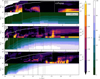 |
Fig. 1 Mass segregation ratios Λ and masses of NMST most massive stars. The three rows with two grouped plots correspond to the M4, M5, and M6 models. The following descriptions apply to the two plots in each row. Top: mass segregation ratio Λ over time for the NMST most massive stars in each cluster. The vertical dotted white lines indicate the time of collapse, where Rrms reaches a minimum. The solid white lines correspond to the right vertical axis showing the stellar mass of the cluster. Bottom: mass of the NMSTth most massive star in each cluster. The grey vertical lines indicate the formation of a new most-massive star (NMST = 1). As these are often not in the core, the time of formation, particularly in M4, corresponds to a drop in the apparent mass segregation. Note that each cluster was run to ≈ 1.5 tff, leading to different absolute timescales. |
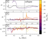 |
Fig. 2 Mass segregation ratio Λ over time for all stars above a given mass threshold MΛ shown on the color bar. Λ is only calculated if there are ≥ 5 stars with mass ≥ MΛ. The threshold for mass segregation is Λ > 1, above the horizontal dashed line. The vertical dotted lines indicate the time of collapse, where Rrms reaches a minimum. Note the variable timescales in each panel. |
4 Discussion
4.1 Timescales
An observed star cluster is determined to have primordial mass segregation if there is mass segregation before the expected segregation timescale of the cluster. A recent study that consistently models individual star formation from gas found that subclusters form primordially segregated (Guszejnov et al. 2022). They do not indicate Λ values for individual stars using NMST, but rather the global Λ for all stars ≥ 5 M⊙. Despite the primordial mass segregation in the sub-clusters, the global Λ still varies as their cluster model evolves. This is in contrast to the results in Allison et al. (2009b) who found that Λ mostly increases after collapse, never decreasing back down to Λ = 1. McMillan et al. (2007) also found in their pure N-body simulations that Λ > 1 values in sub-clusters are retained through mergers. These conflicting results suggest that gas dynamics play a significant role in the long term relaxation and dynamical mass segregation of the cluster.
We calculate the dynamical segregation timescale for our clusters to see when mass segregation occurs with respect to it. The expected time for a star of mass M to dynamically segregate in a uniform spherical cluster is given by (Spitzer 1969; Allison et al. 2009b)
 (2)
(2)
where ⟨ m⋆⟩ and N⋆ are the average mass and number of stars in the cluster,  is the root mean square radius from the center of mass, and σv is the stellar velocity dispersion in the center of mass frame. We note that this is an idealized approximation of the segregation time, as our clusters are far from spherical at early times.
We must address the effect of our mass agglomeration routine on the segregation timescale in our clusters. We agglomerated stars below 4 M⊙. With an IMF sampling mass of 105 M⊙, our agglomeration routine increases ⟨ m⋆⟩ from 0.575 to 5.390 M⊙ and decreases N⋆ from 174432 to 18243. Using Eq. (2), we find that the segregation time of a cluster with agglomeration is 20.6% larger than the segregation time for a cluster without agglomeration. This is an approximation that assumes that agglomeration does not change the radius of the cluster or stellar velocity dispersion. This result means that clusters with the true Kroupa IMF will dynamically mass segregate even more efficiently than our model with the agglomerated IMF. The vast majority of the analysis in this paper calculates Λ for stars with masses ≥ 10 M⊙, while agglomerated stars have mass < 8 M⊙. Because most stars < 10 M⊙ are agglomerated, in a sense measuring mass segregation in our model means comparing the distribution of massive stars to low-mass agglomerate stars. The presence of mass segregation in all our models means that there are more agglomerated stars outside the central cluster region than inside. Therefore, even if we broke up the agglomerated stars into their constituents, our clusters would still have Λ > 1 because the number of low mass stars would still be greater outside the central cluster region.
Figure 3 shows the time evolution of tseg as a function of M for each of the modeled clusters. The mass of the most massive star is indicated by the white line and the grey line shows the evolution of Rrms. In all three clusters, there is a distinct wave pattern of high and low tseg values which correspond to the variations in Rrms during cluster assembly. Over time, N⋆ and σv only increase and ⟨ m⋆⟩ is roughly constant by construction. The segregation time increases as more pockets of dense gas begin to form spatially separate sub-clusters of stars, and decreases when the sub-clusters are pulled together by gravity. The lowest tseg value corresponds to the maximum contraction of the assembling cluster during collapse, after which the cluster expands and tseg increases again.
Comparing Figure 3 to Figure 1 one can see a direct correlation between the episodes of high mass segregation to low segregation times, particularly the time period just after the dense core forms from collapse. This is the mass segregation mechanism described in Allison et al. (2009b) in which the collapse of a star cluster forming from many sub-clusters creates a short-lived dense core that allows for early and efficient dynamical mass segregation in young clusters. They discovered this mechanism with models of N = 1000 star particles initially distributed in sub-clusters. Our model confirms that these results hold for sub-clusters forming self-consistently from the dense substructures in a collapsing cloud. One key difference in our results is that they found Λ to steadily increase after collapse, whereas our clusters show more variability. We suspect this is due to the gas dynamics in our model slowing the relaxation of the star particles.
Starting with the M4 cluster, the first episode of mass segregation is from tcl ≈ 0.8–1.2 Myr, which occurs before tseg begins to increase as more stars form. The final period of steady mass segregation begins at tcl ≈ 3.7 Myr, which is right after the period of low tseg due to the collapse of the cluster. This allows the most massive stars to efficiently reach a state of mass segregation.
The M5 cluster also has an episode of mass segregation when the cluster is young tcl ≈ 0.4 Myr and just after the collapse when tseg is lowest. The collapse induced mass segregation occurs at t = 1.8−2 Myr, just 0.2 Myr after the maximum contraction of the cluster. By the time mass segregation sets in, tseg has risen considerably. At tcl = 1.95 Myr, there is pronounced mass segregation of Λ ≥ 2 for NMST ≤ 20 which corresponds to stellar masses between M = 50−100 M⊙. The segregation timescale for stars in this mass range is between tseg = 2−6 Myr. For stars between M = 50−70 M⊙, tseg = 3−6 Myr which is greater than the age of the cluster. If observing this cluster at that time, one would mistakenly conclude that the massive stars have segregated before the expected dynamical time and therefore must have been primordially segregated. This can occur if observing the cluster just after the initial collapse.
The star formation in M6 is too rapid for mass segregation to set in before multiple sub-clusters form. However, the initial collapse does produce an episode of mass segregation from tcl = 0.56−0.68 Myr. The minimum tseg values due to collapse occurs at tcl = 0.5 Myr. The two most massive stars are segregated before the collapse, and just 0.06 Myr after the maximum contraction the 20 most massive stars become mass segregated as well. The 20 most massive stars (NMST ≤ 20) have M ≥ 90 M⊙. The segregation timescale for these stars during the time period of segregation ranges from tseg = 3−6 Myr. This is again much older than the age of the cluster.
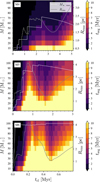 |
Fig. 3 Dynamical segregation time for a star with mass M over time based on the cluster’s properties. The white line indicates the mass of the most massive star, which can decrease due to mass loss from stellar winds. The grey line shows the evolution of the cluster radius Rrms. Note that the dip in the evolution of Rrms indicates the time of collapse. |
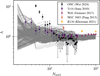 |
Fig. 4 Mass segregation ratio Λ versus number of most massive stars NMST for young Galactic clusters. Each grey line represents one snapshot in time for each of the M4, M5, and M6 clusters. |
4.2 Observational comparisons
The mass segregation ratio Λ for five young clusters in the Milky Way is shown in Figure 4, with the values for our three models indicated in grey. This allows us to assess whether the state of mass segregation observed in these clusters can reasonably be attained with only dynamics. Due to the chaotic nature of star formation and dynamics, we are not expecting an exact match in Λ for a given NMST value. Rather, we are looking to see whether the Λ values in our models reach those seen in observations for a given NMST. For reference, the cluster mass and age of our models and the Milky Way clusters are listed in Table 2.
The degree of mass segregation in the Trumpler 14 (Tr14; Sana et al. 2010), Westerlund 1 (Wd1; Gennaro et al. 2017), and NGC 3603 (Pang et al. 2013) clusters are well within the Λ values of our simulated clusters for the same NMST. Each of these studies concluded that the mass segregation of these clusters can be explained by dynamics and does not have to be primordial because of their segregation timescale. Our results confirm this.
The young massive cluster Radcliffe 136 (R136, see, e.g., Massey & Hunter 1998 or Crowther et al. 2010) embedded in the 30 Doradus star-forming region is mass segregated with Λ ≈ 1.5 at NMST = 50, 100 (Khorrami et al. 2021). At times, our models are slightly segregated at these NMST, with the maximum values reaching Λ ≈ 1.1−1.2. Khorrami et al. (2021) notes that the detection completeness is very low for low-mass stars in the center of the cluster. A young massive cluster such as R136 is likely to have a dense stellar core with many low-mass stars. More low-mass stars in the center of the cluster would lower Λ, so it is probable that these values of Λ are upper limits for R136. With this we conclude that the mass segregation in R136 can be reasonably attained through early dynamics.
All values of Λ in the Orion Nebula Cluster (ONC; Wei et al. 2024) are reached by our model except for the massive Trapezium stars at NMST ≤ 7. Due to the high multiplicity fraction of massive stars (Moe & Di Stefano 2017), it highly likely that the Trapezium stars are binaries rather than single stars. The binaries would undergo mass segregation as a system, increasing Λ for two stars instead of one. We do not include primordial binary formation in our model, which can explain why our models reach the high Λ values seen in the ONC at half the value of NMST.
The Allison et al. (2009b) model, however, did reproduce the mass segregation seen throughout the ONC dynamically. Because of the stochastic nature of star formation and sub-cluster dynamics, our results will vary with different realizations of the initial turbulent seed of the clouds. It is likely that by performing more simulations we would produce a group of NMST = 7 highly centralized stars resembling the Trapezium group.
Wei et al. (2024) find the ONC to be in a super-virial state and expanding. If the ONC formed through hierarchical assembly, the expanding state of the ONC implies that it is post-collapse. This is consistent with the scenario that the ONC became dynamically mass segregated during initial collapse, and is now expanding4. It is also possible that some of the Trapezium stars formed in the center of the ONC if their progenitor gas clumps became mass segregated during collapse.
Up to now, we have compared observations to our model, which has no primordial mass segregation by construction. We find that observations of early mass segregation can be reproduced with no primordial mass segregation. Therefore, to confirm the existence of primordial mass segregation, massive stars must be observed in the center of a cluster as they are forming. Recent ALMA observations of 11 dense protoclusters (Mclump ≥ 103 M⊙) find significant mass segregation of their prestellar and protostellar cores (Xu et al. 2024). This indicates that stars forming within sub-clusters could be primordially mass segregated. If this is the case, as they merge during the collapse of the cluster we expect the mass segregation will only increase. However, it is unclear whether primordially mass segregated sub-clusters remain that way until they merge. Though we do not include pre-main sequence evolution in our models, we see transient periods of dynamical mass segregation in subclusters shortly after they form and before they merge during cluster collapse, which are similar to the primordial segregation seen in the ALMA protoclusters. The concentration of massive stars in the center of a sub-cluster subjects them to a higher chance of being dynamically ejected. With these new results, sub-grid models of star formation should perhaps place massive stars preferentially towards the center of sub-clusters. Then one could determine whether primordial mass segregation persists through the dynamical evolution of the cluster.
Star cluster properties.
5 Conclusions
We performed simulations of star-by-star cluster formation from turbulent self-gravitating gas clouds, taking into account stellar feedback in the form of radiation, stellar winds, and SNe. We find that dynamical mass segregation can occur early on during the hierarchical formation process, when sub-clusters collapse and form a dense core with a much smaller crossing time (as proposed by Allison et al. 2009b for purely stellar dynamical systems).
Due to the hierarchical formation of star clusters, the timescale over which massive stars dynamically segregate tseg varies greatly as the size of the cluster changes. There are two points in a cluster’s lifetime when tseg is significantly lower. First, when the cluster is just forming and only contains a single site of star formation, and second during the initial collapse when the sub-clusters merge into a central cluster forming a short-lived dense core. These two time periods allow massive stars to segregate efficiently, with tseg ≤ 2 Myr for the most massive stars. During initial collapse, the most massive stars in each of our models (≥ 20 M⊙, ≥ 50 M⊙, ≥ 90 M⊙ for M4, M5, M6) underwent efficient mass segregation reaching Λ > 1 within tseg < 0.5 Myr. The variation of tseg over the lifetime of a cluster means that the integrated tseg may be shorter than the value given by the cluster’s current state. Therefore, a young cluster being mass segregated earlier than expected does not necessarily indicate primordial mass segregation.
Mass segregation can occur while star formation is ongoing. This means massive stars and massive star-forming clumps alike will migrate to the center, thereby increasing the likelihood of a massive star being born in the center of the cluster. This can lead to primordial mass segregation if a massive star is formed during the initial collapse of a young cluster.
The mass segregation ratio Λ in young clusters is highly variable due to the ongoing star formation, stellar mass loss, and energetic kinematics of sub-cluster assembly. There are time periods of significant mass segregation in all three clusters that last for 0.1−0.3 Myr. There are also time periods without apparent mass segregation, which usually occur after the dynamical ejection of a massive star from the core. As more massive stars fall into the dense core, they are more likely to be ejected by a strong dynamical encounter. Mass segregation and dynamical ejection are two competing physical processes, and massive stars are most susceptible to both. The interplay and balance of these two processes needs further investigation. Given these variations in Λ before the cluster is fully relaxed, it is unclear how long primordial mass segregation would last.
In summary, our results conclusively show that young clusters can become mass segregated through early dynamics. Efficient dynamical mass segregation is achieved when the initial collapse of the star cluster forms a dense core with a much smaller crossing time. We have demonstrated that the degree of mass segregation seen in young Galactic clusters is also seen in our models and can therefore be achieved through dynamics alone. During collapse, massive stars are more likely to form primordially segregated as massive star-forming clumps will also promptly approach the center of mass. Our findings also indicate that Λ is highly variable at early times. New observations point to primordial mass segregation, at least on the sub-cluster scale, so further work is needed to confirm whether primordial mass segregation would survive cluster assembly or dissipate in a model that includes gas dynamics.
Acknowledgements
We thank the referee for their useful comments and insights, one of which led to the addition of Appendix A. B.P. was partly supported by a fellowship from the International Max Planck Research School for Astronomy and Cosmic Physics at the University of Heidelberg (IMPRS-HD). M.-M.M.L., B.P., and E.A. were partly supported by NSF grants AST18-15461 and AST2307950. E.A. and M.-M.M.L. also acknowledge partial support from NASA grant 80NSSC24K0935. C.C.-C. is supported by a Canada Graduate Scholarship – Doctoral (CGS D) from the Natural Sciences and Engineering Research Council of Canada (NSERC). This work used Stampede 2 at TACC through allocation PHY220160 from the Advanced Cyberinfrastructure Coordination Ecosystem: Services & Support (ACCESS) program, which is supported by National Science Foundation grants 21-38259, 21-38286, 21-38307, 21-37603, and 21-38296. The code development that facilitated this study was done on Snellius through the Dutch National Supercomputing Center SURF grants 15220 and 2023/ENW/01498863. S.M.A. is supported by an NSF Astronomy and Astrophysics Postdoctoral Fellowship, which is funded by the National Science Foundation under Award No. AST24-01740; S.M.A. also acknowledges support from NSF Award No. AST20-09679. R.S.K. and S.C.O.G. acknowledge financial support from the European Research Council via the ERC Synergy Grant “ECOGAL” (project ID 855130), from the Heidelberg Cluster of Excellence (EXC 2181 – 390900948) “STRUCTURES”, funded by the German Excellence Strategy, and from the German Ministry for Economic Affairs and Climate Action in project “MAINN” (funding ID 50002206). The team in Heidelberg also thanks The Länd and the German Science Foundation (DFG) for computing resources provided in bwHPC supported by grant INST 35/1134-1 FUGG and for data storage at SDS @ hd supported by grant INST 35/1314-1 FUGG. M.-M.M.L. acknowledges Interstellar Institute’s program “II6” and the Paris-Saclay University’s Institut Pascal for hosting discussions that nourished the development of the ideas behind this work.
Appendix A Isolating dynamical mass segregation
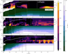 |
Fig. A.1 Mass segregation ratios Λ and masses of NMST most massive stars for an older subset of the stellar populations. Same as Figure 1, but only considering stars formed before 0.75 tcollapse, indicated by the red dotted line. The three rows correspond to the M4, M5, and M6 models as labeled. In each row: (top) mass segregation ratio Λ over time for the NMST most massive stars in each cluster. The vertical dotted white lines indicate the time of collapse, where Rrms reaches a minimum. The solid white lines correspond to the right vertical axis showing the stellar mass of the cluster. (bottom) mass of the NMSTth most massive star in each cluster. The grey vertical lines indicate the formation of a new most-massive star (NMST = 1). As these are often not in the core, the time of formation, particularly in M4, corresponds to a drop in the apparent mass segregation. Note that each cluster was run to ≈ 1.5tff, leading to different absolute timescales. |
Star formation continues during core collapse, so it must be determined whether ongoing star formation or stellar dynamics drives mass segregation during collapse. We do this by repeating the mass segregation analysis for only stars formed before 0.75 tcollapse. Comparing Figure A.1 to Figure 1, respectively, it is clear that dynamical mass segregation is occurring even without the aid of ongoing star formation placing massive stars in the center of the cluster.
The mass segregation of old stars in M4 is almost identical to all stars. This is because the most massive star to form in M4 is created before the 0.75 tcollapse cutoff. The old population in M5 becomes well segregated after collapse across all NMST = 100 stars considered. A few stars more massive than any in the old population form after 0.75 tcollapse, so the high Λ at low NMSt reached in the complete population is not seen when considering the old population. M4 and M5 both indicate that these clusters segregate dynamically without significant aid from stochastic massive star formation in the central cluster during collapse.
The older stars in M6 become much more segregated than the stars that are newly formed. M6 provides a better constraint for this test than M4 and M5, as the mass population of stars formed before and after 0.75 tcollapse is comparable. This allows us to directly compare the degree of mass segregation for stars formed before and during collapse. The result that older stars in M6 become more mass segregated than young stars confirms that dynamics is the dominant mechanism segregating our young clusters during core collapse.
References
- Allison, R. J., Goodwin, S. P., Parker, R. J., et al. 2009a, MNRAS, 395, 1449 [Google Scholar]
- Allison, R. J., Goodwin, S. P., Parker, R. J., et al. 2009b, ApJ, 700, L99 [Google Scholar]
- Baczynski, C., Glover, S. C. O., & Klessen, R. S. 2015, MNRAS, 454, 380 [CrossRef] [Google Scholar]
- Bate, M. R., Bonnell, I. A., & Price, N. M. 1995, MNRAS, 277, 362 [Google Scholar]
- Blaauw, A. 1961, Bull. Astron. Inst. Netherlands, 15, 265 [NASA ADS] [Google Scholar]
- Colella, P., & Woodward, P. R. 1984, J. Computat. Phys., 54, 174 [NASA ADS] [CrossRef] [Google Scholar]
- Crowther, P. A., Schnurr, O., Hirschi, R., et al. 2010, MNRAS, 408, 731 [Google Scholar]
- Federrath, C., Banerjee, R., Clark, P. C., & Klessen, R. S. 2010, ApJ, 713, 269 [NASA ADS] [CrossRef] [Google Scholar]
- Fryxell, B., Olson, K., Ricker, P., et al. 2000, ApJs, 131, 273 [CrossRef] [Google Scholar]
- Fujii, M. S., & Portegies Zwart, S. 2011, Science, 334, 1380 [Google Scholar]
- Fujii, M., Iwasawa, M., Funato, Y., & Makino, J. 2007, PASJ, 59, 1095 [NASA ADS] [Google Scholar]
- Gennaro, M., Goodwin, S. P., Parker, R. J., Allison, R. J., & Brandner, W. 2017, MNRAS, 472, 1760 [NASA ADS] [CrossRef] [Google Scholar]
- Goodwin, S. P., Whitworth, A. P., & Ward-Thompson, D. 2004, A&A, 414, 633 [NASA ADS] [CrossRef] [EDP Sciences] [Google Scholar]
- Grudić, M. Y., Guszejnov, D., Hopkins, P. F., et al. 2018, MNRAS, 481, 688 [CrossRef] [Google Scholar]
- Guszejnov, D., Markey, C., Offner, S. S. R., et al. 2022, MNRAS, 515, 167 [NASA ADS] [CrossRef] [Google Scholar]
- Harayama, Y., Eisenhauer, F., & Martins, F. 2008, ApJ, 675, 1319 [Google Scholar]
- Hillenbrand, L. A., & Hartmann, L. W. 1998, ApJ, 492, 540 [NASA ADS] [CrossRef] [Google Scholar]
- Hoogerwerf, R., de Bruijne, J. H. J., & de Zeeuw, P. T. 2000, ApJ, 544, L133 [NASA ADS] [CrossRef] [Google Scholar]
- Khorrami, Z., Langlois, M., Clark, P. C., et al. 2021, MNRAS, 503, 292 [Google Scholar]
- Klessen, R. S., & Burkert, A. 2000, ApJS, 128, 287 [NASA ADS] [CrossRef] [Google Scholar]
- Klessen, R. S., & Glover, S. C. O. 2016, in Saas-Fee Advanced Course, 43, SaasFee Advanced Course, eds. Y. Revaz, P. Jablonka, R. Teyssier, & L. Mayer, 85 [NASA ADS] [CrossRef] [Google Scholar]
- Kolmogorov, A. 1941, Akad. Nauk SSSR Dokl., 30, 301 [Google Scholar]
- Krause, M. G. H., Offner, S. S. R., Charbonnel, C., et al. 2020, Space Sci. Rev., 216, 64 [CrossRef] [Google Scholar]
- Kroupa, P. 2002, Science, 295, 82 [Google Scholar]
- Lada, C. J., & Lada, E. A. 2003, ARA&A, 41, 57 [Google Scholar]
- Larson, R. B. 1981, MNRAS, 194, 809 [Google Scholar]
- Mac Low, M.-M., & Klessen, R. S. 2004, Rev. Mod. Phys., 76, 125 [Google Scholar]
- Massey, P., & Hunter, D. A. 1998, ApJ, 493, 180 [NASA ADS] [CrossRef] [Google Scholar]
- Matus Carrillo, D. R., Fellhauer, M., Boekholt, T. C. N., Stutz, A., & Morales Inostroza, M. C. B. 2023, MNRAS, 522, 4238 [NASA ADS] [CrossRef] [Google Scholar]
- McKee, C. F., & Ostriker, E. C. 2007, ARA&A, 45, 565 [Google Scholar]
- McKee, C. F., & Tan, J. C. 2003, ApJ, 585, 850 [Google Scholar]
- McMillan, S. L. W., Vesperini, E., & Portegies Zwart, S. F. 2007, ApJ, 655, L45 [Google Scholar]
- Miyoshi, T., & Kusano, K. 2005, J. Computat. Phys., 208, 315 [NASA ADS] [CrossRef] [Google Scholar]
- Moe, M., & Di Stefano, R. 2017, ApJS, 230, 15 [Google Scholar]
- Oh, S., & Kroupa, P. 2016, A&A, 590, A107 [NASA ADS] [CrossRef] [EDP Sciences] [Google Scholar]
- Pang, X., Grebel, E. K., Allison, R. J., et al. 2013, ApJ, 764, 73 [NASA ADS] [CrossRef] [Google Scholar]
- Parker, R. J., & Goodwin, S. P. 2015, MNRAS, 449, 3381 [Google Scholar]
- Pelupessy, F. I., van Elteren, A., de Vries, N., et al. 2013, A&A, 557, A84 [NASA ADS] [CrossRef] [EDP Sciences] [Google Scholar]
- Pfalzner, S., & Kaczmarek, T. 2013, A&A, 559, A38 [NASA ADS] [CrossRef] [EDP Sciences] [Google Scholar]
- Polak, B., Mac Low, M.-M., Klessen, R. S., et al. 2024, A&A, 690, A94 [NASA ADS] [CrossRef] [EDP Sciences] [Google Scholar]
- Portegies Zwart, S., & McMillan, S. 2018, Astrophysical Recipes (IOP Publishing), 2514 [Google Scholar]
- Portegies Zwart, S. F., & Verbunt, F. 1996, A&A, 309, 179 [NASA ADS] [Google Scholar]
- Portegies Zwart, S., McMillan, S., Harfst, S., et al. 2009, New Astron., 14, 369 [Google Scholar]
- Portegies Zwart, S. F., McMillan, S. L. W., & Gieles, M. 2010, ARA&A, 48, 431 [NASA ADS] [CrossRef] [Google Scholar]
- Portegies Zwart, S., McMillan, S. L. W., van Elteren, E., Pelupessy, I., & de Vries, N. 2013, Comput. Phys. Commun., 184, 456 [Google Scholar]
- Portegies Zwart, S., Pelupessy, I., Martínez-Barbosa, C., van Elteren, A., & McMillan, S. 2020, Commun. Nonlinear Sci. Numer. Simul., 85, 105240 [Google Scholar]
- Poveda, A., Ruiz, J., & Allen, C. 1967, Bol. Observ. Tonantzintla Tacubaya, 4, 86 [Google Scholar]
- Reggiani, M., Robberto, M., Da Rio, N., et al. 2011, A&A, 534, A83 [NASA ADS] [CrossRef] [EDP Sciences] [Google Scholar]
- Ricker, P. M. 2008, ApJS, 176, 293 [NASA ADS] [CrossRef] [Google Scholar]
- Sana, H., Momany, Y., Gieles, M., et al. 2010, A&A, 515, A26 [NASA ADS] [CrossRef] [EDP Sciences] [Google Scholar]
- Spitzer, Lyman, L. Jr. 1969, ApJ, 158, L139 [NASA ADS] [CrossRef] [Google Scholar]
- Stutz, A. M. 2018, MNRAS, 473, 4890 [NASA ADS] [CrossRef] [Google Scholar]
- Stutz, A. M., & Gould, A. 2016, A&A, 590, A2 [NASA ADS] [CrossRef] [EDP Sciences] [Google Scholar]
- Truelove, J. K., Klein, R. I., McKee, C. F., et al. 1997, ApJ, 489, L179 [CrossRef] [Google Scholar]
- Vázquez-Semadeni, E., González-Samaniego, A., & Colín, P. 2017, MNRAS, 467, 1313 [NASA ADS] [Google Scholar]
- Wall, J. E., McMillan, S. L. W., Mac Low, M.-M., Klessen, R. S., & Portegies Zwart, S. 2019, ApJ, 887, 62 [NASA ADS] [CrossRef] [Google Scholar]
- Wall, J. E., Mac Low, M.-M., McMillan, S. L. W., et al. 2020, ApJ, 904, 192 [Google Scholar]
- Wang, L., Iwasawa, M., Nitadori, K., & Makino, J. 2020, MNRAS, 497, 536 [NASA ADS] [CrossRef] [Google Scholar]
- Wei, L., Theissen, C. A., Konopacky, Q. M., et al. 2024, ApJ, 962, 174 [NASA ADS] [CrossRef] [Google Scholar]
- Xu, F., Wang, K., Liu, T., et al. 2024, ApJS, 270, 9 [NASA ADS] [CrossRef] [Google Scholar]
Not to be confused with the core collapse that occurs at late dynamical times after the star cluster has already assembled.
Version used for this work: https://bitbucket.org/torch-sf/ torch/commits/tag/massive-cluster-1.0
The maximum agglomerate mass of 8 M⊙ comes from the rare case that the agglomerate mass is just under 4 M⊙ and the next star to be agglomerated is also just under 4 M⊙. For example, if the agglomerate mass is 3.9 M⊙, it will be combined with the next star to form that is < 4 M⊙. If this next star is also 3.9 M⊙, then the agglomerated particle will have a mass of 7.8 M⊙
It has also been suggested that the super-virial state of the ONC might be due to a slingshot effect, where oscillations in the gas filament that formed the ONC led to the ejection of the cluster (see Stutz & Gould 2016; Stutz 2018; Matus Carrillo et al. 2023). In this scenario, it is still possible that the initial collapse of the ONC occurred before expulsion by the filament, allowing for the Trapezium stars to efficiently migrate to the center.
All Tables
All Figures
|
Fig. 1 Mass segregation ratios Λ and masses of NMST most massive stars. The three rows with two grouped plots correspond to the M4, M5, and M6 models. The following descriptions apply to the two plots in each row. Top: mass segregation ratio Λ over time for the NMST most massive stars in each cluster. The vertical dotted white lines indicate the time of collapse, where Rrms reaches a minimum. The solid white lines correspond to the right vertical axis showing the stellar mass of the cluster. Bottom: mass of the NMSTth most massive star in each cluster. The grey vertical lines indicate the formation of a new most-massive star (NMST = 1). As these are often not in the core, the time of formation, particularly in M4, corresponds to a drop in the apparent mass segregation. Note that each cluster was run to ≈ 1.5 tff, leading to different absolute timescales. |
| In the text | |
|
Fig. 2 Mass segregation ratio Λ over time for all stars above a given mass threshold MΛ shown on the color bar. Λ is only calculated if there are ≥ 5 stars with mass ≥ MΛ. The threshold for mass segregation is Λ > 1, above the horizontal dashed line. The vertical dotted lines indicate the time of collapse, where Rrms reaches a minimum. Note the variable timescales in each panel. |
| In the text | |
|
Fig. 3 Dynamical segregation time for a star with mass M over time based on the cluster’s properties. The white line indicates the mass of the most massive star, which can decrease due to mass loss from stellar winds. The grey line shows the evolution of the cluster radius Rrms. Note that the dip in the evolution of Rrms indicates the time of collapse. |
| In the text | |
|
Fig. 4 Mass segregation ratio Λ versus number of most massive stars NMST for young Galactic clusters. Each grey line represents one snapshot in time for each of the M4, M5, and M6 clusters. |
| In the text | |
|
Fig. A.1 Mass segregation ratios Λ and masses of NMST most massive stars for an older subset of the stellar populations. Same as Figure 1, but only considering stars formed before 0.75 tcollapse, indicated by the red dotted line. The three rows correspond to the M4, M5, and M6 models as labeled. In each row: (top) mass segregation ratio Λ over time for the NMST most massive stars in each cluster. The vertical dotted white lines indicate the time of collapse, where Rrms reaches a minimum. The solid white lines correspond to the right vertical axis showing the stellar mass of the cluster. (bottom) mass of the NMSTth most massive star in each cluster. The grey vertical lines indicate the formation of a new most-massive star (NMST = 1). As these are often not in the core, the time of formation, particularly in M4, corresponds to a drop in the apparent mass segregation. Note that each cluster was run to ≈ 1.5tff, leading to different absolute timescales. |
| In the text | |
Current usage metrics show cumulative count of Article Views (full-text article views including HTML views, PDF and ePub downloads, according to the available data) and Abstracts Views on Vision4Press platform.
Data correspond to usage on the plateform after 2015. The current usage metrics is available 48-96 hours after online publication and is updated daily on week days.
Initial download of the metrics may take a while.