| Issue |
A&A
Volume 530, June 2011
|
|
|---|---|---|
| Article Number | A86 | |
| Number of page(s) | 27 | |
| Section | Catalogs and data | |
| DOI | https://doi.org/10.1051/0004-6361/201116504 | |
| Published online | 16 May 2011 | |
The Hubble Legacy Archive ACS grism data
1
Space Telescope – European Coordinating Facility, Karl-Schwarzschild-Str. 2, 85748 Garching, Germany
e-mail: This email address is being protected from spambots. You need JavaScript enabled to view it.
2
Università degli Studi di Milano, Dipartimento di Fisica via Celoria 16, 20133 Milano, Italy
Received: 12 January 2011
Accepted: 23 March 2011
Abstract
A public release of slitless spectra, obtained with ACS/WFC and the G800L grism, is presented. Spectra were automatically extracted in a uniform way from 153 archival fields (or “associations”) distributed across the two Galactic caps, covering all observations to 2008. The ACS G800L grism provides a wavelength range of 0.55−1.00 μm, with a dispersion of 40 Å/pixel and a resolution of ~80 Å for point-like sources. The ACS G800L images and matched direct images were reduced with an automatic pipeline that handles all steps from archive retrieval, alignment and astrometric calibration, direct image combination, catalogue generation, spectral extraction and collection of metadata. The large number of extracted spectra (73,581) demanded automatic methods for quality control and an automated classification algorithm was trained on the visual inspection of several thousand spectra. The final sample of quality controlled spectra includes 47 919 datasets (65% of the total number of extracted spectra) for 32 149 unique objects, with a median iAB-band magnitude of 23.7, reaching 26.5 AB for the faintest objects. Each released dataset contains science-ready 1D and 2D spectra, as well as multi-band image cutouts of corresponding sources and a useful preview page summarising the direct and slitless data, astrometric and photometric parameters. This release is part of the continuing effort to enhance the content of the Hubble Legacy Archive (HLA) with highly processed data products which significantly facilitate the scientific exploitation of the Hubble data. In order to characterize the slitless spectra, emission-line flux and equivalent width sensitivity of the ACS data were compared with public ground-based spectra in the GOODS-South field. An example list of emission line galaxies with two or more identified lines is also included, covering the redshift range 0.2 − 4.6. Almost all redshift determinations outside of the GOODS fields are new. The scope of science projects possible with the ACS slitless release data is large, from studies of Galactic stars to searches for high redshift galaxies.
Key words: methods: data analysis / space vehicles: instruments / techniques: imaging spectroscopy / surveys
© ESO, 2011
1. Introduction
Slitless spectroscopy is primarily a survey tool and most of the use on HST has been with this aim. On account of the lack of selection of target(s) by a slit, then the spectra of all objects in a given field are recorded, implying that the range of targets can be large – from the nearest stars to the most distant galaxies. The primary disadvantages of slitless spectroscopy in comparison with slit spectroscopy are the mutual contamination of spectra, the higher sky background (as compared to imaging) and the range in spectral resolution dictated by the size of the dispersing objects (“virtual slits”). Since early in its history HST has been equipped with instruments capable of slitless spectroscopy (for an overview see Walsh et al. 2010), but the most-used modes have been on NICMOS and ACS and, since Servicing Mission 4, WFC3.
Overview of the provenance of the ACS/G800L data released in the HLA.
As part of the Hubble Legacy Archive (HLA) project to create well-calibrated science data and make them accessible via user-friendly archives, the Space Telescope European Coordinating Facility (ST-ECF) has exploited its expertise in slitless spectroscopy to uniformly extract spectra from widely used slitless spectroscopy modes and to serve the high level science data products through an archive. The HLA is a collaboration between Space Telescope Science Institute (STScI), the Canadian Astronomy Data Centre (CADC) and the ST-ECF. In the first part of this project about 2500 spectra from the NICMOS G141 grism, covering the wavelength range 1.10 to 1.95 μm, were extracted and made publicly available (http://hla.stsci.edu/STECF.org/archive/hla/). The process of extraction, the limitations of the data served and examples of a few of the spectra are described in Freudling et al. (2008). In this paper we present the second part of that project in which all the ACS G800L slitless data taken with the Wide Field Channel (WFC) were extracted and the data products released through the HLA. The ACS G800L grism can also be used with the High Resolution Channel (HRC) and a separate release of slitless spectroscopy in the Hubble Ultra Deep Field was made (see Walsh et al. 2004, and http://archive.stsci.edu/prepds/udf/stecf_udf/HRCpreview.html), but is not considered here.
The bulk (76% by number of pointings, 70% by exposure time) of the ACS G800L spectroscopy was taken in four programmes, two of which were pure parallel. Table 1 presents an overview by proposal of the contents of the HLA ACS slitless spectra, listing the number of associations and grism exposure time. The ACS Pure Parallel Lyα Emission Survey (APPLES, Proposal No. 9482, PI: J. Rhoads) used the ≥ 3 orbit parallel opportunities to obtain a direct image and multiple grism images. Depending on the length of the parallel opportunity, F850LP, F606W and F435W images were added to the core F775W direct image. Low Galactic latitude pointings (|b| > 20°) were avoided. A very similar parallel programme – the ACS Grism Parallel Survey of Emission-line Galaxies at Redshift z < 7 – was also performed in HST Cycle 11 (9468, PI: L. Yan). Results from some deeper pointings (> 12 ks) were reported for 11 high Galactic latitude fields; 601 compact emission-line galaxies at z ≤ 1.6 were found from Hα, Hβ + [O III] and [O II] lines (Drozdovsky et al. 2005).
The Grism-ACS Program for Extragalactic Science (GRAPES, 9793, PI: S. Malhotra) was a primary programme to obtain deep grism exposures in the Hubble Ultra Deep Field (HUDF). The strategy and data reduction is fully described in Pirzkal et al. (2004) and a deep G800L image from another primary programme in the same field was included in the analysis (proposal 9352, PI: M. Riess; see Riess et al. 2004, for results on a supernova at redshift z = 1.3). The strategy adopted for GRAPES was to use the very deep HUDF imaging to provide the positions of the sources to be extracted, and to use comparably short (700s) direct image exposures in F606W to align the grism images to the HUDF catalogue. A range of science was published from these data including detections of faint Galactic stars (Pirzkal et al. 2005) and a grouping of high-z galaxies (Malhotra et al. 2005). A set of 1400 extracted spectra (with i < 27.0 mag) are publicly available at http://archive.stsci.edu/prepds/grapes/
The GRAPES observations were extended to larger fields with the PEARS programme (Probing Evolution And Reionization Spectroscopically, proposal 10530, PI: S. Malhotra), including the Hubble Deep Field North (HDFN) as well as the Chandra Deep Field South (CDFS). Short F606W images were employed to match the coordinates to the Great Observatories Origins Deep Survey (GOODS) catalogue (Giavalisco et al. 2004). Results on emission line galaxies (Straughn et al. 2009), early type galaxies (Ferreras et al. 2009) and faint stars (Pirzkal et al. 2009) have been published. Spectra from PEARS (4082 for the CDF-N field and 5469 for the CDF-S) are publicly available through a searchable interface at http://archive.stsci.edu/prepds/pears/.
Whilst around 10 000 spectra have been publicly released from the GRAPES and PEARS programmes, this represents a small fraction of the available ACS G800L slitless data. Following on from the HLA NICMOS slitless archive, and taking account of recent developments in the slitless extraction software, a uniform reduction of all the ACS G800L slitless data, including GRAPES and PEARS data, presents strong advantages in terms of a homogeneous and well-characterized survey. There are also a number of differences between the extraction of ACS spectra as compared to NICMOS spectra (Freudling et al. 2008) that are highlighted in this paper. Not least for this project was the twenty-fold increase in the number of extracted spectra. Techniques were developed for assessment of the content and quality of the released spectra, also employing machine learning algorithms. Section 2 describes the steps of data collection and reduction: basic processing, catalogue generation, wavelength and flux calibration and quality control. Section 3 describes the empirical characterization of the extracted spectra by reference to ground-based spectra, principally in the GOODS fields. Section 4 covers a description of the released products and some comparisons with ground-based VLT spectra from the ESO-GOODS survey, and the paper closes with a summary. An Appendix lists redshifts and line identifications for selected emission line galaxies with two or more detected lines.
2. Image processing and target selection
2.1. Data preparation
As a preparatory step, the data from the HST archive were grouped into so-called “associations” before processing them. An association is composed of a set of grism and direct images satisfying a set of rules described below. The process of building associations was carried out in three steps: (1) identification of sets of grism images with similar properties; (2) selection of a direct image for each grism image; (3) identification of complementary direct imaging in several bands.
For the first process, we defined two grism images as “compatible” if all the following conditions were fulfilled:
-
HST was using the same guide stars for the grism exposures: thisensures very good relative astrometry between the two images(cf. Sect. 2.3 below);
-
the two grism images have roll angle differences below one degree: this ensures that the dispersed spectra overlap when the data are stacked and any correction for rotation is small;
-
the images have an overlapping area larger than 50% of the whole field: this ensures that a significant fraction of the objects are observed in both exposures justifying the summing of spectra to obtain deeper data.
Additionally, two grism images not satisfying all criteria above were still considered as “compatible” if there was a chain of compatible grism images according to the conditions above. This means that two grism images A and B were still compatible if there exists e.g. an image C which is compatible with both. In mathematical terms, we added a-posteriori a transitivity property to the above relation, which together with the reflexive and symmetric properties defines an equivalence relation, that, finally, was used to define an equivalence class made of compatible grism images.
For each single grism frame, all the direct image frames satisfying the same set of criteria described above were identified. Among these images, the one showing the smallest offset from each grism image was selected to be used in the spectral extraction for the astrometric calibration of each grism frame. Finally, we collected all images (in different filters) which had an overlap of at least 25% of the ACS field with the union of all grism frames. This set of images was used to create the reference image of the association and images in individual bands.
Since the archive search was restricted to science images with a full read out on both detectors, it was not necessary to impose a lower limit for the grism exposure time. As a result of the maximum roll angle difference within an association, the survey fields from programmes such as GRAPES and PEARS, that had multiple roll angles for each telescope pointing as part of their design, were split up into several associations per field.
By following these rules, the grouping of all the ACS G800L grism pointings resulted in 153 fields almost randomly distributed across the two Galactic caps. Figure 1 shows the distribution of these pointings and a summary of each association is given in Table A.3. For each association pertinent details such as the equatorial and Galactic coordinates, the orientation on the sky (the orientation of the y-axis in the detection image) and the direct imaging filter and exposure times together with the number of extracted spectra appearing in the release are listed. A number of grism datasets did not meet these criteria to be included in the final list of associations for processing; they are listed in Table A.1 together with the reasons for exclusion.
2.2. Pipeline processing of the data
The Pipeline for the Hubble Legacy Archive grism data (PHLAG) was used for the end-to-end data processing of all associations. The PHLAG version for processing NICMOS G141 data (Freudling et al. 2008) was further developed to optimally deal with ACS data. The core component of this pipeline is the spectral extraction software aXe which was developed by the ST-ECF to reduce the slitless mode data of HST (Kümmel et al. 2009a). The data reduction is done in a series of processing steps which include:
-
data preparation (see Sect. 2.1);
-
data retrieval from the archive (see Sect. 2.2.1);
-
removal of cosmic rays on direct imaging using the LACOS algorithm (see Sect. 2.2.2);
-
re-alignment of the direct images (see Sect. 2.2.2);
-
MultiDrizzle of the direct images in the available filters (see Sect. 2.2.3);
-
object detection with SExtractor (see Sect. 2.2.4);
-
spectral extraction with aXe (see Sect. 2.2.5);
-
metadata assembly and generation of the archive data products (see Sect. 2.2.7);
-
production of the quality control plots (see Sect. 2.3.1).
In the following we give a brief description of the various processing steps.
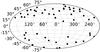 |
Fig. 1 Distribution in Galactic coordinates of the 153 ACS grism associations included in the release. Many associations are very close to each other and thus not discernible individually. |
2.2.1. Pre-processing of ACS data
The basis of the data reduction in PHLAG are standard calibrated images reduced with the CALACS pipeline (Hack 1999). For slitless spectroscopic images, CALACS applies only a basic calibration (correction for bias, dark and gain). Direct images are also flat-fielded in CALACS. We have used data reduced with CALACS version 5.0.4, and for each PHLAG run all images were retrieved from the ST-ECF HST archive cache (Stoehr et al. 2009).
2.2.2. Re-alignment of the direct images
In order to improve alignment of the direct images, the STSDAS task tweakshifts (Koekemoer et al. 2006) was run on the ensemble of direct images of each association. tweakshifts performs an object detection algorithm on the ACS images and then determines the residual shift (no rotation was allowed) by matching the objects on the direct images. In order to minimize the number of false detections due to cosmic rays we run the LACOS algorithm (van Dokkum 2001) on all direct images prior to tweakshifts. LACOS was run as an PyRAF/IRAF task with the parameters sigclip=4.5, sigfrac=0.3, objlim=3.5 and niter=4. The code of tweakshifts was customized to be able to determine shifts up to 30 pixel, in contrast to ~3 pixel in the standard version.
2.2.3. Co-addition of undispersed images
In each association the direct images were grouped according to the filter and then co-added to create a deep image in each filter (with a scale of 0.05 arcsec/pixel). This image combination is done with the MultiDrizzle software (Koekemoer et al. 2006). We also combine the dispersed image in order to detect the cosmic ray affected pixels in the MultiDrizzle processing. As in direct imaging MultiDrizzle is able to detect cosmics appearing in individual exposures and does not extinguish real, compact object signatures such as emission lines and zeroth order beams that appear in each image. The co-added grism image from this operation was not further used in the processing.
2.2.4. Target catalogue
The first step in the extraction of slitless spectra is to find objects on the undispersed image (Kümmel et al. 2009a). Object parameters required for the extraction are the coordinates, the axis lengths and the position angle of the major axis.
We used the SExtractor program (Bertin & Arnouts 1996) to generate the object catalogues. For the object detection we generated a deep, “white light” image by co-adding all available deep filter images, using the exposure time maps as weights. The photometric information in the filter images is obtained by using SExtractor in double-image mode (Bertin 2008), whereby one image (the “white light” image) is used for the object detection and a second image (a filter image) for photometry. For all images the exposure time maps generated in the co-addition step were used as a weight map to reduce spurious detections and improve the photometric accuracy.
Relevant SExtractor parameters used for the source extraction on the detection image.
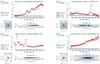 |
Fig. 2 Examples of ACS grism spectra as shown in the previews included in the release. Blue curves (when present) indicate the estimated contamination from near-by sources as a function of wavelength. The green data points (horizontal bars) correspond to the integrated broad band magnitudes. The blue rectangular box in the 2D spectrum shows the effective extracted region where the extraction was performed. In the cutout direct image (taken from the “white light” detection image), the “pseudo-slit” and the dispersion direction are indicated (blue arrow). Top left: an M-star; top right: a low redshift star burst galaxy; bottom left: a broad-absorption line QSO identified as a Chandra X-ray source at z = 2.78 (Szokoloy et al. 2004); bottom right: an early-type galaxy. |
The detection list and the photometric lists were combined, and the resulting catalogue was filtered to remove spurious objects and bad photometry:
-
we removed spurious objects that were detected but have nophotometric information;
-
we removed spurious objects that were extremely large (
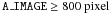 ) or very large and with a high ellipticity (
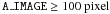 and
and  );
); -
inaccurate photometric measurements (
 ) were discarded.
The relevant parameters used for the object detection with SExtractor are given in Table 2.
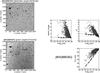 |
Fig. 3 Quality control for association J8HBBOKQ I: the detection image and the co-added grism image (left side); statistical analysis of the object parameters from the detection list (right side). The upper left panel shows the object size, the upper right panel the stellarity parameter s2 (Pirzkal et al. 2009) and the lower right panel the central surface brightness as a function of object brightness. The solid and dotted lines mark the exact locus of point-like objects and the enclosing tolerance area, respectively. |
2.2.5. Spectral extraction
The extraction of spectra from the dispersed images was done with the aXe spectral extraction software (Kümmel et al. 2009a). The reduction strategy chosen follows closely the extraction for the NICMOS G141 data as outlined in Freudling et al. (2008). Many of the features developed for that project have been included into the standard aXe software, and the ACS grism reduction was done using the version 1.71 of aXe. Among the processing steps taken, are:
-
the sky background was removed by subtracting a scaled mastersky background image from the science data. The area covered bythe spectra of objects in the master object list was excluded whendetermining the scale factor;
-
the extraction direction for each object was chosen to optimize the spectral resolution as outlined in Freudling et al. (2008) and Kümmel et al. (2010). Objects with
 (= 0.055 arcsec) on the detection image were treated as point-like, which means
  and the extraction direction set perpendicular to the dispersion direction1;
 -
the contamination of the extracted spectra from neighbouring sources was estimated using a model of the dispersed image. The latter was generated by adopting the simplest SED for every pixel belonging to an object using the fluxes derived from the direct images (the so called “fluxcube” model, see Kümmel et al. 2010);
-
the spectra on the individual grism images were re-binned to a linear scale in wavelength and spatial direction and then co-added to deep, 2D grism image stamps. The 1D spectra were then extracted from these co-added image stamps (aXedrizzle, see Kümmel et al. 2010);
-
extended sources, which here are all objects with a virtual slit width larger than the 1.1 pix attributed to point like objects (see above), were flux calibrated using a Gaussian smoothed version of the sensitivity function (Freudling et al. 2008; Kümmel et al. 2010).
2.2.6. Aperture correction
The extraction as described above uses optimized virtual slits that adjust the slit length to the object morphology. The lower limit for the object sizes and the chosen scaling parameter in aXe (parameter outfwhm in the task axedrizzle) result in a minimal aperture with a half-width of 3.3 pixel or 0.165 arcsec. For the minimal aperture the fraction of the total object flux included in the spectrum can be calculated from the wavelength dependence of the aperture correction listed in Table 3 (from Kuntschner et al. 2008). Using these values, all extracted spectra were corrected to the total object flux. Since the aperture correction in Kuntschner et al. (2008) was derived from standard star observations, this procedure results in the total flux only for point-like objects and represents only a lower limit for extended sources.
Fraction of the total flux extracted for point-like objects.
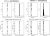 |
Fig. 4 Quality control for association J8HBBOKQ II: results from fitting Gaussians to the spatial profile of the 2D stamp images for bright, compact sources. The left side shows the offset of the center from the expected position, the right side shows the profile width. |
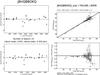 |
Fig. 5 Quality control for association J8HBBOKQ III: the wavelength offset for M-stars identified by cross-correlating extracted spectra with M-star templates (left side). A comparison of the direct imaging magnitudes and the “spectral magnitudes” derived by integrating the spectra over the corresponding filter throughput curve (right side). The comparison of the direct image magnitudes derived with a finite aperture and the “spectral magnitudes” that were computed from the aperture corrected spectra (see Sect. 2.2.6) results in an offset from the zero line. |
2.2.7. Generation of archive data products
From the extracted spectra and the co-added filter images, the following data products are generated to be distributed via the HLA archive:
-
The 1-dimensional spectrum as in FITS table format, followingthe data formatting specified for FITS serialization by theIVOA Spectral Data Modelversion 1.03 (McDowell &Tody 2007). Each data point contains thewavelength in Å, the count rate in electrons per second and the flux expressed in physical units along with associated errors and an estimate of the contaminating flux, i.e. the sum of the flux from all other sources whose spatial and spectral extent overlaps with that of the extent of the extracted source. Additional metadata include keywords to describe the contamination, the orientation of the dispersion direction on the sky and “footprints”, i.e. the spatial extent on the sky of the extraction region given by the height of the extraction aperture and the image size of the source (from the SExtractor image parameters) in the dispersion direction.
-
The co-added, 2D grism image as a multi-extension FITS file. The various extensions contain the grism stamp image, its error array, the exposure time map and the contamination map.
-
The direct image stamp as a multi-extension FITS file. It contains the cutout images (5′′ × 5′′) and the corresponding weight images from the detection image and all available direct imaging.
-
The preview image such as shown in Fig. 2. The preview combines all basic results in a single image. It contains a spectrum plot with contamination estimate and broad band magnitudes, the 2D grism stamp indicating the extraction region and the direct image with the orientation on the sky and an illustration of the extraction geometry. The extraction length in the cross-dispersion direction and the dispersion direction are also indicated.
The error in the 1-dimensional extracted spectra is based on error propagation from the error array in the ACS images through the final spectra. Thus it contains CCD related errors (readout noise, poisson noise) and flux calibration errors. Errors from flat-fielding and sky background subtraction are more difficult to quantify on a pixel-to-pixel basis, and have been taken into account by setting a minimum error threshold of 1% of the flux.
The contaminating flux, as estimated from the modelling of neighouring objects, should help to estimate the level of contamination in the extracted flux and hence to identify clean spectral regions for scientific exploitation.
2.3. Astrometric calibration and accuracy
2.3.1. Quality control of the PHLAG output
The quality of the PHLAG output is automatically monitored. This is done by analyzing for each association the products of PHLAG, primarily the co-added direct images, the source lists and the extracted spectra. The results are stored as a series of plots representing a particular aspect. Figures 3 − 5 show the following quality control plots produced for the association J8HBBOKQ:
-
A plot of the whole detection image and the co-added grism imagegives an overview on the field of view and identifies possibleproblems due to e.g. stray light (left side ofFig. 3).
-
The plot on the right side of Fig. 3 analyzes the size distribution of the detected objects. It summarizes the object extent (upper left panel), the stellarity parameter s2 (upper right panel; the ratio of the flux within a circular aperture of radius 1 pixel to the total isophotal flux as measured by SExtractor, see Pirzkal et al. 2009) and the central surface brightness as a function of source brightness (lower right panel). The locus of point-like objects is marked with the dotted parallel lines, and problems in the re-alignment of direct images result in an offset from this locus, and were readily apparent. The quality flag attributed to each association in Table A.3 is mainly based on this plot.
-
For each 2D grism stamp image the cross-dispersion profile was extracted and fitted by a number of Gaussians at different wavelengths. Possible offsets of the spectrum centres from their nominal position (Fig. 4, left side) or large widths (Fig. 4, right side) point to alignment problems between the slitless images and their associated direct images.
-
M-stars were identified by cross-correlating the 1D-spectra of point-like objects (from the SExtractor catalogue) with a set of M-star templates taken from the BPGS atlas (Gunn et al. 1983). Since the zeropoint of the wavelength calibration depends on an accurate translation of the object position from the direct to the slitless images, a wavelength offset (see Fig. 5, left side) identified in the M-stars would point to alignment problems between the grism images and their associated direct images.
-
The 1D-spectra are integrated over all direct imaging filters (if the filter passband was covered by the wavelength range of the spectra). These “spectral magnitudes” are then compared to an aperture magnitude derived from the filter images. The right side of Fig. 5 shows such a comparison for compact objects of one association and the F814W filter. While brightness differences of ≈ 0.15 mag as shown in Fig. 5 are expected due to the usage of aperture corrected spectra but finite photometric apertures, larger differences or even systematic trends identify problems in either the direct imaging or the spectra extraction.
On the basis of these plots problems were identified on an association by association basis and corrected prior to production of the final release data. As a result of the quality control, the following rules were defined in order to ensure homogeneous quality for the products of all associations:
-
a minimum of 2 grism images in an association is required;
-
a minimum of 2 direct images in one filter is required for an association;
-
direct images that could not be re-aligned with the tweakshift tasks (see Sect. 2.2.2) were discarded;
-
the direct imaging in the filters blue-wards of the slitless spectrum range (F435W, F475W and F555W) are discarded if the re-alignment or the co-adding failed;
-
associations with an object density higher than 2000 per square arcminute are discarded, since in this case overlap of spectra is such that the majority of spectra are multiply contaminated and there is insufficient background region available for background estimation;
-
the accuracy of the background subtraction for the grism data was monitored. Grism images with large residuals, e.g. due to stray light from a bright star or a low surface brightness contribution from a large galaxy, were discarded. As a result, some associations taken close to M31 could not be reduced (see Table A.1);
Table 4Reference catalogues used for astrometric calibration.
-
significant offsets either in the spatial direction or in the wavelength direction as identified in Figs. 4 and 5 were translated into shifts of the object position and applied. E.g. for the association J8HQBBOKQ the offsets −0.45 pixel and +0.25 pixel had been applied in x- (spectral-) and y- (spatial-) direction, respectively. In general, shifts in x-direction were applied if at least 5 M-stars could be identified for an association and the shift was greater than 0.25 pixel with 2-σ significance. Shifts in the y-direction were applied if larger than 0.25 pixel.
As a result of this first quality control process, 15 associations were discarded and hence not included in this release, leaving the total of 153 associations shown in Fig. 1 (see Tables A.1 and A.3).
The astrometric coordinate system of the raw ACS images is specified in the WCS keywords in the image headers. The accuracy is ultimately limited by the accuracy of the guide catalogue used for pointing the telescope. For earlier data, the Guide Star Catalog I (Lasker et al. 1990) was used, and since 2000 the Guide Star Catalog II (McLean et al. 2000) is used. The absolute accuracy reaches 0.3 arcsec over a large fraction of the sky, but errors can be as high as several arcseconds towards the edges of the scanned plates. Additionally, misidentification of sources or confusion effects can, in some cases, create inaccuracies in the raw ACS astrometry as large as 10 arcsec.
In order to improve the astrometric accuracy of the ACS direct images, and thus of the sources associated to released spectra, we cross-correlated source catalogues extracted from the ACS fields with several reference astrometric catalogues: UCAC2, 2MASS, SDSS-DR6, USNO-B1, GSC2.3.2, and the GOODS WFI R-band catalogue where relevant (see Table 4). When multiple matches were found, the most accurate of these catalogue was used. The fitting procedure allows for simple shifts of the astrometry, but not for rotation which we found to be generally negligible in HST observations. We used several techniques to avoid false matches, including sigma-clipping and cluster analysis; we also introduced magnitude cuts for each astrometric catalog (so that, for example, a 2MASS star would not match an object of R mag of 22).
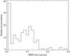 |
Fig. 6 Residual astrometric errors after WCS calibration. |
We evaluated the astrometric accuracy of each association from the standard dispersion of all offsets measured between objects found in the association and the corresponding matched reference objects from the astrometric catalogs. While the residual errors are equally distributed in RA and Dec, Fig. 6 shows the histogram of its absolute value for all associations after applying the WCS calibration. The error depends strongly on the number and quality of the matches obtained, but in any case should provide a good upper limit to the actual accuracy of the astrometric solution. As can be seen in Fig. 6, the accuracy for the large majority of the fields is below 0.2 arcsec (with median error 0.15 arcsec). This accuracy is confirmed by a check in the GOODS fields where accurate (50 mas) astrometry is available.
2.4. Wavelength calibration
In-orbit wavelength calibration for G800L spectra was established by observations of the Wolf-Rayet star WR96 and verified with observations of the planetary nebula LMC-SMP-81 (programmes 9568 and 10058, see Larsen & Walsh 2005). The observations of the Wolf-Rayet star cover 20 independent locations across chip 1 and chip 2 while LMC-SMP-81 was observed at three different positions. The wavelength calibrations were carried out with a direct least-squares fit of the G800L spectra to a (smoothed) spectrum of WR96 obtained from the ground (Pasquali et al. 2006). This approach has the advantage that blends are automatically accounted for, and thus does not rely on the ability to accurately measure the wavelengths of individual spectral features (Larsen & Walsh 2005). With the verification of the wavelength zero point via M-star spectra (see Sect. 2.3.1) the overall absolute wavelength calibration error is estimated to be smaller than 1 pixel, i.e. 40 Å.
2.5. Flux calibration of 1D spectra
The flux calibration for the G800L grism was derived from observations of the primary HST standard star G191B2B at 11 different positions covering both chips of ACS and cross-checked with observations of the standard star GD153 (programmes 9029, 9568 and 10374, see Kuntschner et al. 2008). The absolute flux calibration of the 1st order G800L spectra for point sources is accurate to better than 2% for the spatial positions covered by the standard stars and wavelengths from 6000 to 9500 Å. Including errors from the large scale flat-field, the absolute calibration is better than 5% for point sources.
2.6. Duplicate spectra
Several grism pointings overlap, in all areas of the sky, and in particular in the GOODS-S field resulting from the GOODS and PEARS programmes. This offers an opportunity to test the robustness of the reduction and extraction routines. We thus searched the complete catalogue of released spectra, including 47 919 spectra in 153 associations, for companion spectra within a five arcsecond radius. We then plotted the radial distribution of the companion spectra, and found a clear break at ~0.3″. We choose this as the radius within true matches are to be found. In the total sample, 32 149 objects have unique spectra and 8185 have duplicate spectra, ranging from a single pair of duplicates, to up to 13 spectra of the same object. ~ 40% of all the duplicate spectra are in the GOODS-S field and ~20% in the HUDF.
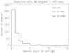 |
Fig. 7 Median σ of all spectral bins of each pair of spectra, where both spectra have low contamination, and the roll angle between the two measurements is > 40°. |
For the test of the accuracy of the data reduction and extraction, duplicate spectra with contamination <20% in the whole spectral range were selected. Further, to test the most extreme cases, only duplicates where the roll angle differences between observations was >40° were compared. No constraint was put on the size of the object. The significance on the agreement between the two spectra was calculated as the median significance (σ) of the difference between the two spectra, weighted with the error on each spectrum, over all wavelength points. The resulting histogram of median σ is shown in Fig. 7.
Of the spectra measured in this way, 61% had median significances within 1σ, and 10% had values >3σ. The most common reason for a large σ are extremely small error-bars on very bright objects. Overall, the agreement between spectra, even with a large roll angle between the observations, is remarkably good.
2.7. Quality control of extracted spectra
In the pre-release of the ACS/G800L data set in May 2009, which was restricted to two field in the GOODS south area (Kümmel et al. 2009b), the number of extracted spectra was small enough to allow an individual, visual inspection. During this interactive quality control process 40% of the extracted spectra were discarded, which led to the final release of 1235 spectra. The main reasons for the rejection was a high contamination from nearby sources, but also the presence of deviant pixels that are either saturated or lying near the edges of the observed fields.
A visual inspection of the full sample of 73 581 spectra produced in this release was impossible to do on reasonable time-scales. We therefore have explored ways of automatic classification using machine-learning techniques. The idea is to first train an algorithm with a relatively small number of hand-classified spectra using measured values such as the estimated contamination fraction, the signal-to-noise ratio, the magnitude, the position of the maximum of light on the 2D spectrum or the exposure time. In a second step then, ideally the remaining spectra can be classified automatically with the algorithm returning the classification of the spectrum at hand by finding the classification of the most similar spectrum in the training set.
Three of us (JW, HK and PR), acted as quality control scientists, inspecting 2020 (~3% of the total sample) randomly selected spectra from the full sample and classified them independently into “good” and “bad”. The 241 spectra with mismatching classifications were re-examined until a consolidated classification by all three scientists was achieved. This process resulted in a very clean and homogeneously training sample for the automatic classification, which is a key to get high automatic classification success rates.
The automatic classification was then carried out using the weka software package (Hall et al. 2009). The machine learning algorithms were trained with 2/3 of the consolidated training set and the quality of the classification was measured by applying the trained algorithm on the independent remaining 1/3 of the inspected set. Several algorithms showed similar performance for the task at hand. The final algorithm chosen was ClassificationViaRegression using an M5P tree, which resulted in a very high total classification rate (90%). Also the rate of false negatives (“good” spectra classified as “bad”) was only 2.5% and thus very low with this algorithm. This is important as it turned out that there were a surprisingly large percentage of spectra in the sample that are borderline cases (roughly 15%) between the spectra that are unambiguously publishable and those that are not. With the choice of this algorithm we opted to include the spectra into the “good” sample if in doubt. The classification quality of 90% achieved by the algorithm is comparable or even slightly better than the quality that each of the quality control scientists achieved individually when inspecting the training sample.
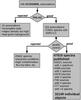 |
Fig. 8 Flow diagram of the data processing and quality control, leading to the released sample of HLA/ACS spectra and related number of individual unique sources. |
The classification algorithm was then run on the 97% of the remaining spectra of the full sample. The 21 416 spectra falling in the “bad” category were discarded. The 50 145 spectra from the “good” category were passed on to post-classification analysis.
During the training of the algorithm it became apparent that there are classes of spectra that are clearly flawed but are classified by the algorithm as “good”. The reason for this is that the number of such cases in the training sample is too small for the algorithm to build up expertise. We call such spectra “catastrophic failures”.
One such class of spectra is characterized by saturated centers (67 spectra). A second class of 1628 spectra displays dramatically raising SED’s at both ends of the spectral range, which is caused by an underestimated object size and thus a too narrow smoothing kernel in the flux calibration (see Sect. 2.2.5). These classes of spectra could be identified via specific detection algorithms, and their small number allowed a visual inspection and selection of all members.
The remaining set of “good” spectra was then looked-at by concatenating 100 previews into a poster-like web interface for rapid inspection. 1951 spectra (i.e. 4% of the remaining sample) were discarded in this process resulting in a total of 47 919 “good” spectra. The effort for skimming through these spectra was roughly equivalent to that of carefully classifying the training set. The machine classification therefore saved more than 90% of the time that would have had to be spent on a complete visual classification. The entire data processing and quality control process of associations and spectra which lead to the final released sample of ACS HLA spectra is summarized in the flow diagram shown in Fig. 8. The magnitude distribution of the 32 149 unique sources is shown in Fig. 9.
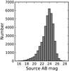 |
Fig. 9 Magnitude distribution of the 32 149 individual sources associated to the HLA/ACS spectra. AB F775W magnitudes are used for most of the objects. |
2.8. Comparison of spectra with VLT data
Twenty-nine grism pointings are located within the GOODS-S field (Giavalisco et al. 2004), where many reduced spectra from other surveys are publicly available. This allows the comparison of our spectra with ground based spectra of the same objects as an external quality control. The catalogues of spectra used in this test come from the ESO/VLT FORS spectrograph (Szokoloy et al. 2004; Vanzella et al. 2008) and from the ESO/VLT VIMOS instrument (Le Fevre et al. 2004; Balestra et al. 2010).
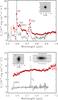 |
Fig. 10 Comparison of the ACS grism spectra (data points with error bars) with ground-based spectra (gray lines). Upper panel: the source HAG_J033209.44-274806.8 identified as a broad absorption line QSO at z = 2.81 by Szokoloy et al. (2004) using VLT/FORS2 spectroscopy with the 150I grism (see Fig. 2 for the full preview image). Lower panel: the source HAG_J033239.83-275652.8, a spiral galaxy at z = 0.125, identified with a VLT/FORS2 spectrum taken with the 300I grism as part of the ESO-GOODS survey (Vanzella et al. 2008). The insets show the direct image stamps and, in the lower panel, also the 2D slitless stamp image. |
For this test, the difference between all the FORS and VIMOS spectra, rebinned and convolved with the resolution profile of the grism spectrum, and their corresponding grism spectra were compared to the combined errors on the grism spectra and on the ground-based spectra, as calculated by the function DER_SNR (Stoehr et al. 2008). All points in the spectra with contamination less than 10% were used. The median significance of this difference is shown in Fig. 11 for the total sample of 926 matched spectra. The figure also shows the same result divided into four sub-samples of spectra; the GOODS-S FORS spectra, the VVDS VIMOS spectra, the GOODS-S VIMOS spectra and the FORS spectra of CDFS X-ray sources. Of the 926 matched spectra, 14% have median significances better than 1σ, 46% are better than 3σ and 76% are better than 10σ. Considering that no corrections are made to match or correct aperture sizes of the slitless and slit spectra, or other systematic effects due to spectral feature, the agreement is reasonably good. Two examples are shown in Fig. 10. The upper panel shows the UV rest-frame of a quasar whose broad lines are clearly detected in the grism spectrum. Also the overall flux levels agree reasonably well with each other. In the case of the low-redshift spiral galaxy (lower panel), the narrow emission lines (unresolved in the ground-based spectrum with R = 660) remain undetected in the grism spectrum, whereas the mismatch in the continuum flux is the result of aperture effects. As can be seen in the inset showing the 2D grism stamp plus the extracted region (blue box), the slitless aperture is with 2.5′′ much larger than the 1′′ used for the FORS2 slit spectrum.
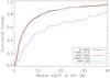 |
Fig. 11 Median σ of all wavelength points of matched ground-based and grism spectra, excluding points with large contamination. Black line shows the distribution of all 926 spectra, and the coloured lines mark the various sub-samples (see text). 92 spectra have a median significance > 25σ. |
3. Empirical characterization of emission line sensitivities
We have seen how slitless spectroscopy is affected by contamination, the spectral resolution is generally low and is further degraded for extended sources depending on their size, all aspects that differ from typical slit spectroscopy and make a direct assessment of limiting sensitivities difficult. An assessment of the flux continuum and line limits, redshift accuracy, etc. can be made by resorting to well-studied samples of objects in common with ground-based spectra at faint magnitudes in the GOODS South field.
Common targets were found in two steps. Firstly, matching objects were found within 1 arcsec radii. If multiple matches were possible within this search radius, the closest match was retained. Secondly, due to the overlap of several grism pointings, a cleaning algorithm was applied to remove multiple entries of the same source. This procedure produced 1237 matched sources distributed over 356 FORS spectra, 641 VIMOS spectra and 240 spectra from other surveys. For this characterization, we will focus on the FORS and VIMOS spectra. A plot of the redshift distribution of the FORS/VIMOS matched sources can be found in Fig. 12. The distributions follow the overall distribution of ground-based determined redshifts, i.e. the selection of objects in redshift space was on average uniform and random. The drop in objects above z ~ 1.5 is thus an artifact of declining galaxy number densities, and spectroscopic incompleteness in the ground-based spectra.
Before measuring emission-line fluxes, the ground-based spectra were convolved with the PSF profile of the G800L grism, also taking into account the extraction aperture size of the corresponding grism spectrum. This ensures a matched resolution in the ground-based and grism spectra. An automatic script was then used to fit Gaussian functions to any emission-lines present in the wavelength range 5500 − 9500 Å. The redshift was assumed to be that given for the ground-based spectrum, and the line flux and EW were calculated from the Gaussian fit. Measurements were only made in regions where the contamination in the grism spectrum was less than 20%. Given the uncertainty in slit losses, the flux density in the ground-based spectrum in the region around the line was normalized to that in the grism spectrum. Due to these uncertainties, as well as the effect of varying aperture sizes (see below), we focus here on the emission-line fluxes, as opposed to equivalent width (EW). The result was stored and is shown as gray points in Fig. 13.
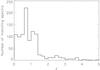 |
Fig. 12 Redshift distribution of grism sources with ground-based spectra from the FORS and VIMOS surveys. |
Even though a relation between the ground-based and grism fluxes is seen, the agreement is not as good as expected. A reason for a disagreement could be that emission-line regions can be small and localized within larger galaxies. The pipeline will automatically set an extraction aperture incorporating the whole galaxy, effectively smearing the emission-line flux out. This would decrease the apparent line flux compared to the ground-based measurement, as is apparent in Fig. 13. To test this, and to compensate for it, new one-dimensional spectra were extracted from the two-dimensional extraction stamps in varying aperture sizes (see also http://hla.stsci.edu/STECF.org/archive/hla/indiv_extraction.php). The emission-lines in these spectra were then re-measured and the process iterated until the best matches to the ground-based spectra were found. The results of this test are shown with red points in Fig. 13, and display a much better correlation between ground-based and grism measurements. Before the optimization, 58% of the measured line fluxes disagreed with more than 2σ, the majority of those having too low fluxes as measured in the grism spectra. After the optimization, the percentage of >2σ discrepancies dropped to 9%, with roughly equal number of objects with too high/low flux as measured in the grism spectrum, consistent with random scatter. It is clear that a refinement of the extraction is necessary, particularly so in the case of more extended objects. In Fig. 14 the results are plotted as a function of size and total magnitude of the objects.
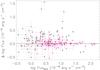 |
Fig. 13 Difference in the emission-line flux measured in the ground-based (GB) and the grism spectra (ACS) (Δlog Flux = log FluxGB − log FluxACS) as a function of the ACS emission-line flux. Grey/red points are before/after a tailored extraction. Only lines with ≥ 3σ detections in both measurements are shown. The solid line indicates a 1:1 relation. Points above the solid line indicate too low flux measurements in the grism spectra. |
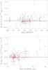 |
Fig. 14 Difference (Δlog Flux as in Fig. 13) in measured line fluxes as a function of overall magnitude in the z band (top) and major axis length as determined in the white light image (bottom). Grey points are results before optimization and red after. Arrows in the upper plot indicate objects with upper limits on their magnitudes. The largest improvement is for large/bright objects, as expected. |
Larger objects have, before optimization, the largest offsets between ground-based and grism line measurements but are in good agreement after optimization. Thus, the best improvement in the agreement is achieved with larger objects. These objects also tend to be brighter overall, and a strong improvement in the agreement is also seen for bright objects in Fig. 14. It is important to note that the line flux result after optimization was designed to match the line flux of the ground-based spectrum, and is not necessarily the “true” line flux. The line flux/EW measured from a grism spectrum can vary greatly, depending on extraction size, and location of extraction centre. Thus, slitless spectra offer an opportunity to study spatially resolved line emission for bright objects.
The measurements made here can be used to calculate an empirical sensitivity limit to emission lines in G800L observations. To study this, the 3σ significant measurements were divided into three bins depending on exposure time of the spectrum, with texp > 16 000 s, 10 000 < texp ≤ 16 000 s and texp ≤ 10 000 s. The histogram of fluxes measured in the grism spectra for these three bins are shown in Fig. 15. To calculate an empirical detection limit, the 80% completeness limit in each sub-sample was found in the cumulative distribution. The limits measured are log FluxACS = (−16.24, −16.08, −15.82) erg s-1 cm-2 for the bins with mean exposure time of (20 510,15 030,4320) s. For these exposure times, and assuming a Gaussian line with 100 Å width and a S/N = 3, the limiting line fluxes reached according to the ACS Exposure time calculator (ETC, see http://etc.stsci.edu/etc/input/acs/spectroscopic/) are log Flux = (−16.70, −16.52, −16.30) erg s-1 cm-2. These values are significantly fainter than the empirical limits found above, although the ETC values depend on several factors, such as line EW, line central wavelength, extraction size etc. If only the faintest detected values in Fig. 15 are taken into account, the minimum fluxes reached are log FluxACS = (−16.43, −16.31, −16.12) erg s-1 cm-2, more in agreement with the ETC values.
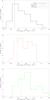 |
Fig. 15 Histogram of ACS line fluxes, from top to bottom as a function of decreasing exposure time. The median exposure times are 20 510 s in the top panel, 15 030 s in the middle panel and 4320 s in the bottom panel. The solid vertical lines mark the 80% completeness limit in each sub-sample. |
Finally, in Fig. 16 the histogram of line fluxes is shown for different size bins. The results in the figure confirm that the limiting flux is size dependent. The 80% completeness in the two size sub-samples are log FluxACS = (−16.18, −15.70) erg s-1 cm-2 for the bins with sizes less/greater than five pixels.
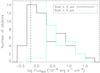 |
Fig. 16 Histogram of ACS line fluxes, divided into size bins of A_IMAGE in pixel as measured on the detection image. Solid vertical lines mark the 80% completeness limit in each sub-sample. |
4. Data distribution
HLA data are distributed by both ST-ECF and STScI and there are several ways to access the ACS spectra:
-
Archive Query Interface. HLA grism spectra can be searched onthe dedicated HLA grism spectra interface(http://archive.eso.org/wdb/wdb/hla/product_science/form)that allows many constraints on target (e.g. thetarget name), the data properties (e.g. effectiveexposure time), the source properties(e.g. the magnitude) and the data quality(e.g. the signal-to-noise ratio). Also the generalHST query interface at http://archive.eso.org/hst/scienceincludes all grism spectra, however with a less specific interface.
-
Archives at CADC and STScI. The ST-ECF HLA data has been also integrated into the general search interface at CADC (http://cadc.hia.nrc.gc.ca/hst/) as well as into the HLA interface of the STScI (http://hla.stsci.edu). The footprints of the equivalent slits of the grism spectra are also included into their footprint service.
-
Virtual Observatory. We provide fully automated access to the HLA metadata and data via Virtual Observatory (VO) standards. A Simple Spectrum Access Protocol (SSAP) server has been established (http://stecf.org/hst-vo/). It serves VOTables in V1.1 format, which contain, in addition to the standard metadata, information about the footprints of the equivalent slits of the grism spectra. Our SSAP and SIAP server have been tested with ESOs archive browser VirGO (http://archive.eso.org/cms/virgo/) as well as with SPLAT (http://star-www.dur.ac.uk/~pdraper/splat/splat-vo/) and VOSpec (http://esavo.esac.esa.int/vospec/).
5. General considerations for space-based slitless surveys
Over the last decade, a number of space-based all-sky slitless surveys have been designed with the aim of measuring baryonic acoustic oscillations in the 3D-distribution of galaxies (e.g. Glazebrook et al. 2005; Wang et al. 2010). Space-based slitless experiments in the near-IR take advantage of the low-background (~1000 times lower than on the ground) and can cover wide areas with high sensitivity. Galaxy redshift surveys conducted in this way can measure the large number of redshifts (> 107 emission line galaxies) needed to constrain the dark energy equation of state parameter to a 1% level, particularly in the redshift interval 1 ≲ z ≲ 2, which is very hard to access from the ground. Such experiments are part of the Euclid ESA mission (Laureijs et al. 2009), which is currently in the definition phase, as well as of the JDEM mission concept.
The large archive of ACS G800L spectra prepared in this work represents a unique collection of space-bourne slitless spectra and may prove useful in the planning of future slitless surveys from space. Expertise developed in the course of supporting ACS, and WFC3, slitless spectroscopy and the uniform reduction of ACS G800L spectra, described here, fed directly into simulations for the NIR slitless survey with Euclid, which featured in the Euclid Study Report (“The Yellow Book”; ESA 2009).
ACS G800L data has a spectral resolution of about 80 for point sources and is adequate for redshift determination of emission line sources, spectral typing of stars and even modelling of late-type galaxy spectra (e.g. Ferreras et al. 2009). WFC3 NIR grisms have higher spectral resolution; the 2.6 times larger projected pixel size compared to ACS present some advantages in determining the redshift of single small (≤ 0.3′′) objects, but not, for example, for disentangling the spectra of larger objects with complex structure (such as late-type galaxies with HII regions). WFC3 NIR grism surveys published over the next few years will however be very useful for projecting the performance of future dark energy surveys that will be operating in the 1 − 2 μm range and use primarily Hα as a redshift indicator (e.g. Atek et al. 2010).
As emphasized in Sect. 1, the contamination of spectra is one of the most serious disadvantages of slitless spectroscopy as compared to multi-object slit spectroscopy. Its effect requires to be mitigated as much as possible in order to ensure a good return of clean spectra from a given slitless survey. The exact level of contamination depends on the target density, thus on the Galactic latitude at the largest scale, and the length of the spectra on the detector. Other considerations that influence the contamination are the presence of multiple orders (including zeroth order, where the similarity to an emission line for a point source can be a significant hindrance in surveys relying on emission line redshifts) and the relative strength of these orders with respect to the primary order (usually that carrying the most power). In the case of the ACS G800L, some contamination seriously affected around 40% of the extracted spectra. The ubiquity of contamination in slitless spectroscopy implies that strategies for dealing with contaminated spectra are a necessary part of the reduction process and should be folded into the analysis.
For HST slitless surveys, the aim has been to provide as accurate as possible assessment of the likely effect of contamination on any given spectrum. The method developed for HST slitless spectra has relied upon morphological and spectral information from direct imaging. A direct image is mandatory for defining the wavelength zero point for each extracted spectrum and plays a critical role in defining the size of the extraction (the virtual slit) and the effective resolution of a given slitless spectrum set by the object size projected in the dispersion direction. Thus one direct image is the minimum requirement for the slitless spectroscopy, but the availability of more than one image improves the contamination estimate by providing colour(s) of targets and a crude SED. Drop-out objects (containing a continuum break) are a particular case in point, since with only one image their contaminating flux must be, by default, assumed to be constant in flux and thus the extent of the contamination will be over-estimated. The use of the surface brightness distribution for extended sources (flux cube contamination – Kümmel et al. 2009a) rather than a 2D Gaussian fit, adds to the fidelity of the contamination estimation and directly to the yield of spectra with well-described contamination. The degree to which contamination can be well described clearly plays an important role in the fidelity of redshift determination.
The fraction of uncontaminated spectral pixels for a given object clearly rises with the number of distinct rolls angles. For ACS the GRAPES (Pirzkal et al. 2004) and PEARS surveys both had a minimum of 3 position angles. This observational strategy was found to allow the fraction of contaminated spectra (defined as below some level for a given fraction of pixels) to be approximately halved with four roll angles. The question of how to combine slitless spectra at different roll angle is however a complex one: for extended objects the spectra can differ radically depending on the projection of the virtual slit and cannot be simply averaged. Indeed the GRAPES and PEARS surveys distributed the spectra at different rolls angles as separate files. Only in the case of point or marginally extended sources should slitless spectra be averaged. For all targets this is really only justified on the basis of a given scientific analysis. Even for point sources, spectra from different rolls can contain different mixes of contaminating spectra, so combination after contamination removal must be contemplated before combination of spectra.
The flow diagram in Fig. 8 shows that 35% of the total number of extracted spectra were rejected in the course of the learning process. Conservative estimates suggest that this would fall to about half with four rolls angles, but general conclusions for other instruments must depend on dispersion, number and strength of orders, spatial pixel scale, etc. Detailed simulations using the available tools (such as aXeSIM, Kümmel et al. 2009a), for typical fields are required to determine the exact return from multiple rolls, as was performed for the Euclid survey (e.g. Geach et al. 2010).
6. Summary and conclusion
As part of the effort to enhance the content of the Hubble archive, we have extracted slitless spectroscopic spectra taken with the ACS/WFC G800L grism in 153 archival fields which are distributed over the entire sky. Using a fully automated data processing pipeline, we extracted 73 581 spectra with a wavelength of 0.55 − 1.00 μm and a dispersion of 40 Å/pixel from the grism images. An automatic classification algorithm, trained by the visual inspection of a test sample, was used for the quality control. This algorithm selected 47 919 “good” spectra for publication that were derived from 32 149 unique objects with a median iAB-band magnitude of 23.7. Every released 1D spectrum is accompanied with a 2D grism stamp spectrum, a direct image cutout in the available bands and a preview image summarizing the results. All data is distributed through a dedicated query interface and through VO access protocols.
The released grism spectra are science-ready, and many science cases can be addressed with these spectra. Slitless spectra have been shown to be successful tools in finding and studying Galactic stars (e.g. Pirzkal et al. 2009). They also can be used to study emission-line galaxies such as described in Sect. 3 and Appendix A (see also e.g. Malhotra et al. 2005; Straughn et al. 2009, 2011). Other higher redshift science cases involve studying continuum features of high redshift galaxies such as the UV slope at z > 3.5. Nilsson et al. (2011) show the fitting of the spectral energy distributions of a set of low redshift Lyman-break (z ~ 1) galaxies combining both photometric data points and ACS slitless spectra.
The experience accumulated with data from the slitless-modes of HST, such as the HLA data set described here, will be very useful when quantifying the performance of future space based slitless experiments.
While true point like sources on ACS/WFC images have lower values  , slightly extended sources would not profit from an extraction adjusted for extended objects, hence the choice of 1.1 pixel as the lower limit.
Acknowledgments
This paper is based on observations made with the NASA/ESA Hubble Space Telescope, obtained from the data archive at the Space Telescope – European Coordinating Facility. We thank our HLA collaborators Brad Whitmore and the STScI and CADC HLA teams.
References
- Adelman-McCarthy, J. K., Agüeros, M. A., Allam, S. S., et al. 2007, ApJS, 172, 634 [NASA ADS] [CrossRef] [Google Scholar]
- Atek, H., Malkan, M., McCarthy, P., et al. 2010, ApJ, 723, 104 [NASA ADS] [CrossRef] [Google Scholar]
- Balestra, I., Mainieri, V., Popesso, P., et al. 2010, A&A, 512, A12 [NASA ADS] [CrossRef] [EDP Sciences] [Google Scholar]
- Barger, A. J., Cowie, L. L., Brandt, W. N., et al. 2002, AJ, 124, 1839 [NASA ADS] [CrossRef] [Google Scholar]
- Barger, A. J., Cowie, L. L., & Wang, W.-H. 2008, ApJ, 689, 687 [NASA ADS] [CrossRef] [Google Scholar]
- Bertin, E. 2008, The SExtractor Manual, http://www.astromatic.net/software/sextractor [Google Scholar]
- Bertin, E., & Arnouts, S. 1996, A&A, 117, 393 [Google Scholar]
- Drozdovsky, I., Yan, L., Chen, H.-W., et al. 2005, AJ, 113, 1324 [NASA ADS] [CrossRef] [Google Scholar]
- Ferreras, I., Pasquali, A., Malhotra, S., et al. 2009, ApJ, 706, 158 [NASA ADS] [CrossRef] [Google Scholar]
- Freudling, W., Kümmel, M., Haase, J., et al. 2008, A&A, 490, 1165 [NASA ADS] [CrossRef] [EDP Sciences] [Google Scholar]
- Geach, J. E., Cimatti, A., Percival, W., et al. 2010, MNRAS, 402, 1330 [NASA ADS] [CrossRef] [Google Scholar]
- Giavalisco, M., Ferguson, H. C., Koekemoer, A. M., et al. 2004, ApJ, 600, L93 [NASA ADS] [CrossRef] [Google Scholar]
- Glazebrook, K., Baldry, J., Moos, W., et al. 2005, New Astron. Rev., 49, 374 [NASA ADS] [CrossRef] [Google Scholar]
- Gunn, J. E., & Stryker, L. L. 1983, ApJS, 52, 121 [NASA ADS] [CrossRef] [Google Scholar]
- Hack, W. 1999, STScI, ISR ACS, 1999-03 [Google Scholar]
- Hall, M., Frank, E., Holmes, G., et al. 2009, The WEKA Data Mining Software: An Update, SIGKDD Explorations, 11 [Google Scholar]
- Koekemoer, A. M., Fruchter, A. S., Hook, R. N., et al. 2006, The 2005 Calibration Workshop, ed. A. Koekemoer, P. Goudfrooij, & L. Dressel, 423 [Google Scholar]
- Kümmel, M., Kuntschner, H., & Walsh, J. R. 2007, Space Telescope – European Coordinating Facility Newsletter, 43, 8 [Google Scholar]
- Kümmel, M., Walsh, J. R., Pirzkal, N., Kuntschner, H., & Pasquali, A. 2009a, PASP, 121, 59 [NASA ADS] [CrossRef] [Google Scholar]
- Kümmel, M., Rosati, P., Kuntschner, H., et al. 2009b, ST-ECF Newsletter, 46, 6 [Google Scholar]
- Kümmel, M., Walsh, J., & Kuntschner, H. 2010, The aXe Manual, ST-ECF [Google Scholar]
- Kuntschner, H., Kümmel, M., & Walsh, J. R. 2008, ST-ECF ISR ACS, 2008-01 [Google Scholar]
- Larsen, S. S., & Walsh, J. R. 2005, ST-ECF ISR ACS, 2005-08 [Google Scholar]
- Lasker, B. M., Sturch, C. R., McLean, B. J., et al. 1990, AJ, 99, 2019 [NASA ADS] [CrossRef] [Google Scholar]
- Laureijs, R., et al. 2009, ESA/SRE(2009)2 [arXiv:0912.0914] [Google Scholar]
- Le Fevre, O., Vettolani, G., Paltani, S., et al. 2004, A&A, 428, 1043 [NASA ADS] [CrossRef] [EDP Sciences] [Google Scholar]
- Malhotra, S., Rhoads, J. E., Pirzkal, N., et al. 2005, ApJ, 626, 666 [NASA ADS] [CrossRef] [Google Scholar]
- McDowell, J., & Tody, D. 2007, IVOA Spectral Data Model Version 1.01, http://www.ivoa.net/Documents/PR/DM/SpectrumDM-20070515.html [Google Scholar]
- McLean, B. J., Greene, G. R., Lattanzi, M. G., & Pirenne, B. 2000, Astronomical Data Analysis Software and Systems IX, 216, 145 [Google Scholar]
- Monet, D. G., Levine, S. G., Canzian, B., et al. 2003, AJ, 125, 984 [NASA ADS] [CrossRef] [Google Scholar]
- Nilsson, K. K., Möller-Nilsson, O., Rosati, P., et al. 2011, A&A, 526, 10 [NASA ADS] [CrossRef] [EDP Sciences] [Google Scholar]
- Pasquali, A., Pirzkal, N., Larsen, S., Walsh, J. R., & Kümmel, M. 2006, PASP, 118, 270 [NASA ADS] [CrossRef] [Google Scholar]
- Pirzkal, N., Xu, C., Malhotra, S., et al. 2004, ApJS, 154, 501 [NASA ADS] [CrossRef] [Google Scholar]
- Pirzkal, N., Sahu, K. C., Burgasser, A., et al. 2005, ApJ, 622, 319 [NASA ADS] [CrossRef] [Google Scholar]
- Pirzkal, N., Burgasser, A. J., Malhotra, S., et al. 2009, ApJ, 695, 1591 [NASA ADS] [CrossRef] [Google Scholar]
- Riess, A. G., Strolger, L.-G., Tonry, J., et al. 2004, ApJ, 600, L163 [NASA ADS] [CrossRef] [Google Scholar]
- Skrutskie, M. F., Cutri, R. M., Stiening, R., et al. 2006, AJ, 131, 1163 [NASA ADS] [CrossRef] [Google Scholar]
- Stoehr, F., Fraquelli, D., Kamp, I., et al. 2007, ST-ECF Newsletter, 42, 4 [Google Scholar]
- Stoehr, F., White, R., Smith, M., et al. 2008, in Astronomical Data Analysis Software and Systems XVII, ed. R. W. Argyle, P. S. Bunclark, & J. R. Lewis, ASP Conf. Ser., 394, 505 [Google Scholar]
- Stoehr, F., Durand, D., Haase, J., & Micol, A. 2009, in Astronomical Data Analysis Software and Systems XVIII, ed. D. Bohlender, D. Durand, & P. Dowler, ASP Conf. Ser., 411, 155 [Google Scholar]
- Straughn, A. N., Pirzkal, N., Meurer, G. R., et al. 2009, AJ, 138, 1022 [Google Scholar]
- Straughn, A. N., Kuntschner, H., Kümmel, M., et al. 2011, AJ, 141, 14 [NASA ADS] [CrossRef] [Google Scholar]
- Szokoloy, G. P., Bergeron, J., Hasinger, G., et al. ApJS, 155, 271 [Google Scholar]
- van Dokkum, P. 2001, PASP, 113, 1420 [NASA ADS] [CrossRef] [Google Scholar]
- Vanzella, E., Cristiani, S., Dickinson, M., et al. 2008, A&A, 478, 83 [NASA ADS] [CrossRef] [EDP Sciences] [Google Scholar]
- Walsh, J. R., Kümmel, M., & Larsen, S. S. 2004, ST-ECF Newsletter, 36, 8 [Google Scholar]
- Walsh, J. R., Kuntschner, H., & Kümmel, M. 2010, in Proceedings of the 2010 HST Calibration Workshop, STScI, Baltimore [Google Scholar]
- Wang, Y., Percival, W., Cimatti, A., et al. 2010, MNRAS, 409, 737 [NASA ADS] [CrossRef] [Google Scholar]
- Wirth, G. D., Willmer, C. N. A., Amico, P., et al. 2004, AJ, 127, 3121 [NASA ADS] [CrossRef] [Google Scholar]
- Zacharias, N., Urban, S. E., Zacharias, M. I., et al. 2004, AJ, 127, 3043 [NASA ADS] [CrossRef] [Google Scholar]
Appendix A: Multiple line emitters
If no other information is available for a celestial object, typically two or more emission-lines observed in a spectrum will suffice to determine the redshift of the source. With this goal in mind, i.e. determining redshifts for objects, all grism spectra were searched for double or multiple emission lines within the same spectrum. Note that it is not in the scope of this publication to create an exhaustive list of emission-line redshifts. This section is merely meant as an introduction to the method, and interested users may find more objects using other selection criteria. The criteria for selection for follow-up used here were the following:
-
1:
only the wavelength region 5600–9500 Å was considered.
-
2:
only spectral points with contamination less than 10% of the flux were considered.
-
3:
only spectral points with flux greater than 4σ significance after subtraction of the continuum (fitted with a second degree polynomial) were considered.
-
4:
at least three adjacent spectral points satisfying criterion 3 had to be found in each of the two wavelength regimes 5700 − 7400 Å and 7600 − 9300 Å.
-
a visual inspection adjusted the parameters above to the optimal selection, i.e. minimising false detections, and rejected some bad spectra.
Table A.1List of failed associations.
-
6:
finally, spectra of duplicate objects (in different associations) were excluded by matching the locations within 1′′.
A selection with these criteria will allow detection of strong line emitters in the redshift ranges of z = 0.158 − 0.417 for the combination Hβ/[OIII]/Hα, z = 0.529 − 0.857 for [OII]/Hβ/[OIII] and z ~ 3.9 − 5.0 for Lyα/CIV. The selected sample consisted
of 54 objects. For these 54 the obvious emission-lines were fitted with Gaussian functions to retrieve the central wavelength of the lines. From these central wavelengths, redshifts were determined. We report these determinations, including spectral IDs and line identifications in Table A.2.
The redshift and its significance intervals reported in the table are determined from the central wavelengths (and uncertainties thereof) of the Hα or the [OII] lines when available. For the Lyα emitters the redshift is the mean from all measured lines in the spectrum and the uncertainty is the standard deviation on those measurements. Note that the uncertainties are in the fitting of the Gaussian line, and do not include systematic uncertainties due to e.g. the sizes of the galaxies. Thus they must be considered lower estimates of the uncertainties. Allowing a potential systematic error of 1 spectral pixel (40 Å) would for instance result in a δz = [0.006, 0.011, 0.033] for [Hα, [OII], Lyα]. It may also be possible for users to find more multiple line emitters, if allowing smaller significances on the emission line fluxes (see criterion 3 above), larger spectral intervals (criteria 1 and 4 above) or relaxing the contamination criterion.
9 of the objects in Table A.2 are located in the GOODS fields, and around ~ 80% of them have already published redshifts. Outside of the GOODS fields only four sources have already published redshifts. The four sources with large differences between our redshift estimates and the published values are discussed in the Notes to Table A.2.
Objects with determined redshifts.
The associations included in this release.
All Tables
Relevant SExtractor parameters used for the source extraction on the detection image.
All Figures
|
Fig. 1 Distribution in Galactic coordinates of the 153 ACS grism associations included in the release. Many associations are very close to each other and thus not discernible individually. |
| In the text | |
|
Fig. 2 Examples of ACS grism spectra as shown in the previews included in the release. Blue curves (when present) indicate the estimated contamination from near-by sources as a function of wavelength. The green data points (horizontal bars) correspond to the integrated broad band magnitudes. The blue rectangular box in the 2D spectrum shows the effective extracted region where the extraction was performed. In the cutout direct image (taken from the “white light” detection image), the “pseudo-slit” and the dispersion direction are indicated (blue arrow). Top left: an M-star; top right: a low redshift star burst galaxy; bottom left: a broad-absorption line QSO identified as a Chandra X-ray source at z = 2.78 (Szokoloy et al. 2004); bottom right: an early-type galaxy. |
| In the text | |
|
Fig. 3 Quality control for association J8HBBOKQ I: the detection image and the co-added grism image (left side); statistical analysis of the object parameters from the detection list (right side). The upper left panel shows the object size, the upper right panel the stellarity parameter s2 (Pirzkal et al. 2009) and the lower right panel the central surface brightness as a function of object brightness. The solid and dotted lines mark the exact locus of point-like objects and the enclosing tolerance area, respectively. |
| In the text | |
|
Fig. 4 Quality control for association J8HBBOKQ II: results from fitting Gaussians to the spatial profile of the 2D stamp images for bright, compact sources. The left side shows the offset of the center from the expected position, the right side shows the profile width. |
| In the text | |
|
Fig. 5 Quality control for association J8HBBOKQ III: the wavelength offset for M-stars identified by cross-correlating extracted spectra with M-star templates (left side). A comparison of the direct imaging magnitudes and the “spectral magnitudes” derived by integrating the spectra over the corresponding filter throughput curve (right side). The comparison of the direct image magnitudes derived with a finite aperture and the “spectral magnitudes” that were computed from the aperture corrected spectra (see Sect. 2.2.6) results in an offset from the zero line. |
| In the text | |
|
Fig. 6 Residual astrometric errors after WCS calibration. |
| In the text | |
|
Fig. 7 Median σ of all spectral bins of each pair of spectra, where both spectra have low contamination, and the roll angle between the two measurements is > 40°. |
| In the text | |
|
Fig. 8 Flow diagram of the data processing and quality control, leading to the released sample of HLA/ACS spectra and related number of individual unique sources. |
| In the text | |
|
Fig. 9 Magnitude distribution of the 32 149 individual sources associated to the HLA/ACS spectra. AB F775W magnitudes are used for most of the objects. |
| In the text | |
|
Fig. 10 Comparison of the ACS grism spectra (data points with error bars) with ground-based spectra (gray lines). Upper panel: the source HAG_J033209.44-274806.8 identified as a broad absorption line QSO at z = 2.81 by Szokoloy et al. (2004) using VLT/FORS2 spectroscopy with the 150I grism (see Fig. 2 for the full preview image). Lower panel: the source HAG_J033239.83-275652.8, a spiral galaxy at z = 0.125, identified with a VLT/FORS2 spectrum taken with the 300I grism as part of the ESO-GOODS survey (Vanzella et al. 2008). The insets show the direct image stamps and, in the lower panel, also the 2D slitless stamp image. |
| In the text | |
|
Fig. 11 Median σ of all wavelength points of matched ground-based and grism spectra, excluding points with large contamination. Black line shows the distribution of all 926 spectra, and the coloured lines mark the various sub-samples (see text). 92 spectra have a median significance > 25σ. |
| In the text | |
|
Fig. 12 Redshift distribution of grism sources with ground-based spectra from the FORS and VIMOS surveys. |
| In the text | |
|
Fig. 13 Difference in the emission-line flux measured in the ground-based (GB) and the grism spectra (ACS) (Δlog Flux = log FluxGB − log FluxACS) as a function of the ACS emission-line flux. Grey/red points are before/after a tailored extraction. Only lines with ≥ 3σ detections in both measurements are shown. The solid line indicates a 1:1 relation. Points above the solid line indicate too low flux measurements in the grism spectra. |
| In the text | |
|
Fig. 14 Difference (Δlog Flux as in Fig. 13) in measured line fluxes as a function of overall magnitude in the z band (top) and major axis length as determined in the white light image (bottom). Grey points are results before optimization and red after. Arrows in the upper plot indicate objects with upper limits on their magnitudes. The largest improvement is for large/bright objects, as expected. |
| In the text | |
|
Fig. 15 Histogram of ACS line fluxes, from top to bottom as a function of decreasing exposure time. The median exposure times are 20 510 s in the top panel, 15 030 s in the middle panel and 4320 s in the bottom panel. The solid vertical lines mark the 80% completeness limit in each sub-sample. |
| In the text | |
|
Fig. 16 Histogram of ACS line fluxes, divided into size bins of A_IMAGE in pixel as measured on the detection image. Solid vertical lines mark the 80% completeness limit in each sub-sample. |
| In the text | |
Current usage metrics show cumulative count of Article Views (full-text article views including HTML views, PDF and ePub downloads, according to the available data) and Abstracts Views on Vision4Press platform.
Data correspond to usage on the plateform after 2015. The current usage metrics is available 48-96 hours after online publication and is updated daily on week days.
Initial download of the metrics may take a while.