| Issue |
A&A
Volume 529, May 2011
|
|
|---|---|---|
| Article Number | A149 | |
| Number of page(s) | 62 | |
| Section | Extragalactic astronomy | |
| DOI | https://doi.org/10.1051/0004-6361/201016291 | |
| Published online | 22 April 2011 | |
VLT spectroscopy of low-metallicity emission-line galaxies: abundance patterns and abundance discrepancies⋆,⋆⋆
1
Max-Planck-Institute for Radioastronomy, Auf dem Hügel 69, 53121
Bonn, Germany
e-mail: This email address is being protected from spambots. You need JavaScript enabled to view it.
2
Main Astronomical Observatory, Ukrainian National Academy of
Sciences, Zabolotnoho
27, Kyiv
03680,
Ukraine
3
LUTH, Observatoire de Meudon, 92195
Meudon Cedex,
France
4
Institute for Astrophysics, University of Göttingen,
Friedrich-Hund-Platz 1,
37077
Göttingen,
Germany
5 Centro de Astrofísica da Universidade
do Porto, Rua das
Esteral, 4150-762
porto,
Portugal
6
Department of Astronomy, Oskar Klein Centre, Stockholm
University, 10691
Stockholm,
Sweden
Received:
9
December
2010
Accepted:
7
March
2011
Abstract
Context. We present deep spectroscopy of a large sample of low-metallicity emission-line galaxies.
Aims. The main goal of this study is to derive element abundances in these low-metallicity galaxies.
Methods. We analyze 121 VLT spectra of H ii regions in 46 low-metallicity emission-line galaxies. Of these spectra 83 are archival VLT/FORS1+UVES spectra of H ii regions in 31 low-metallicity emission-line galaxies that are studied for the first time with standard direct methods to determine the electron temperatures, the electron number densities, and the chemical abundances.
Results. The oxygen abundance of the sample lies in the range 12 + log O/H = 7.2−8.4. We confirm previous findings that Ne/O increases with increasing oxygen abundance, likely because of a higher depletion of oxygen in higher-metallicity galaxies. The Fe/O ratio decreases from roughly solar at the lowest metallicities to about one tenth of solar, indicating that the degree of depletion of iron into dust grains depends on metallicity. The N/O ratio in extremely low-metallicity galaxies with 12 + log O/H < 7.5 shows a slight increase with decreasing oxygen abundance, which could be the signature of enhanced production of primary nitrogen by rapidly rotating stars at low metallicity. We present the first empirical relation between the electron temperature derived from [S iii]λ6312/λ9069 or [N ii]λ5755/λ6583 and the one derived from [O iii]λ4363/λ(4959+5007) in low-metallicity galaxies. We also present an empirical relation between te derived from [O ii]λ3727/(λ7320 + λ7330) or [S ii]λ4068/(λ6717 + λ6730) and [O iii]λ4363/λ(4959+5007). The electron number densities Ne(Cl iii) and Ne(Ar iv) were derived in a number of objects and are found to be higher than Ne(O ii) and Ne(S ii). This has potential implications for the derivation of the pregalactic helium abundance. In a number of objects, the abundances of C++ and O++ could be derived from recombination lines. Our study confirms the discrepancy between abundances found from recombination lines (RLs) and collisionally excited lines (CELs) and that C/O increases with O/H.
Key words: galaxies: starburst / methods: observational / galaxies: abundances / galaxies: dwarf / galaxies: ISM
© ESO, 2011
1. Introduction
Comprehensive studies of low-metallicity emission-line galaxies in the nearby universe are essential to investigate star formation and galaxy evolution with chemical conditions close to those in the early universe. In particular, studies of abundance ratios and their dependencies on metallicity in low-metallicity galaxies are important for studying the early chemical evolution of galaxies and the nucleosynthesis of massive stars in an environment characterized by a nearly pristine chemical composition. Improved statistics of low-metallicity galaxies, observed with high accuracy, are also important to put observational constraints on the primordial helium abundance, which is a key parameter for testing cosmological models.
We here continue our study of nearby (redshift z ≲ 0.1) star-forming galaxies with measured intensities of the [O iii] λ4363 emission line (Guseva et al. 2006; Izotov et al. 2006; Papaderos et al. 2006; Guseva et al. 2007; Papaderos et al. 2008). This line is important to directly determine the physical conditions and chemical abundances of the ionized interstellar medium.
There were many spectroscopic surveys in the past aiming to study element abundances of nearby low-metallicity emission-line galaxies (e.g. Kunth & Sargent 1983; Campbell et al. 1986; Terlevich et al. 1991; Masegosa et al. 1994; Melbourne & Salzer 2002). However, most of these spectroscopic data are not suitable for our goals for various reasons, such as an insufficient quality of the data, the nonlinearity of the detectors in observations before the 1990ies, and the limited wavelength coverage.
In this paper, we consider archival data from the 8.2 m Very Large Telescope (VLT) obtained in the period 2000−2008 with the spectrographs FORS1 and UVES, which allow us to compile a sample of 83 high-quality spectra of metal-poor H ii regions. We merge this sample with 15 archival VLT/FORS1+UVES spectra of two BCD galaxies, SBS 0335–052E and SBS 0335–052W (Izotov et al. 2009), and VLT/FORS2 spectra of 23 H ii regions in 12 low-metallicity emission-line galaxies from Guseva et al. (2009). We thus obtain a large VLT sample of 121 H ii regions, which includes to our knowledge all high-quality spectra from low-metallicity objects observed with the VLT/UVES+FORS instruments. They are used to study the abundance patterns of low-metallicity emission-line galaxies.
H ii regions and galaxies observed with the VLT.
For comparison reasons we supplemented this sample with 109 low-metallicity emission-line galaxies from the HeBCD sample that were observed with different telescopes and collected by Izotov & Thuan (2004) and Izotov et al. (2004) for the study of the primordial He abundance. The total sample consists of objects with low extinction and in general with a high equivalent width EW(Hβ) of the Hβ emission line, which suggests a young age of the respective starburst. It also includes almost all most metal-deficient galaxies known, which allows for the deepest insights into the abundance pattern of the lowest-metallicity galaxies available in the local Universe. Additionally, we compare abundance patterns of this sample with those of the galaxies from the Data Release 3 (DR3) of the Sloan Digital Sky survey (SDSS) by Izotov et al. (2006) with lower quality spectra but higher metallicity, thus extending the range of oxygen abundances to higher values. H ii regions in the above samples are selected mainly because of their high apparent brightness to obtain high signal-to-noise ratio spectra, and not considering their physical properties, such as the Hβ luminosity. However, these differing selection criteria do not introduce biases. In particular, Izotov et al. (2011) have shown that the abundances and abundance ratios of luminous compact galaxies selected from the SDSS by their high Hβ luminosity do not differ from the samples selected by their apparent brightness.
This paper is organized as follows: in Sect. 2 we describe observations and data reduction. In Sect. 3 we comment on the physical parameters of the H ii regions. In Sect. 4 we discuss the abundance patterns derived from the analysis of collisionally excited lines and present carbon and oxygen abundances obtained from the analysis of recombination lines. We summarize our conclusions in Sect. 5.
2. Observations and data reduction
From the ESO archive we selected VLT spectra of H ii regions that were obtained with the spectrographs UVES (high resolution) and FORS1 (low and medium resolution). The list of the 31 emission-line galaxies to which these H ii regions pertain as well as the two H ii regions NGC 346 and NGC 456 in the Small Magellanic Cloud is given in Table 1 together with the equatorial coordinates, the spectrographs used and the identification number of the ESO program. The total number of spectra from these galaxies available for abundance determinations (and listed in Table 2) is 83 – larger than the list in Table 1. This is because in some galaxies several one-dimensional spectra of H ii regions were extracted from two-dimensional frames. One galaxy, Tol1214–277, was observed with two different spectrographs. Furthermore, the entire objects from the ESO program 69.C-0203(A) were observed with low and medium resolution. Four galaxies were observed twice with VLT/UVES within two different ESO programmes. The images of the observed galaxies overlayed by the slit positions are shown in Fig. 1.
The raw spectra of the objects from the ESO archive as well as the calibration spectra were reduced using IRAF1. The details of data reduction are described in Thuan & Izotov (2005). The two-dimensional spectra were bias subtracted and flat-field corrected. We then used the IRAF software routines IDENTIFY, REIDENTIFY, FITCOORD, and TRANSFORM to perform wavelength calibration and correction for distortion and tilt for each frame. Night sky subtraction was performed using the routine BACKGROUND. The level of night sky emission was determined from the regions closest to the H ii region which are free of stellar and nebular line emission, as well as of emission from foreground and background sources. Exceptions are the extended Small Magellanic Cloud (SMC) H ii regions NGC 346 and NGC 456, for which no night sky subtraction was done. One-dimensional spectra were then extracted from each two-dimensional frame using the APALL routine. Before extraction, distinct two-dimensional spectra of the same H ii region were carefully aligned using the spatial locations of the brightest part in each spectrum, so that spectra were extracted at the same positions in all subexposures. We have summed the individual spectra from each subexposure after removal of the cosmic ray hits.
The high-resolution spectra of H ii regions observed with the UVES spectrograph
are shown in Fig. 2, while low-resolution and
medium-resolution FORS1 spectra are shown in Figs. 3
and 4, respectively. All these figures are available
in electronic form only. Emission-line fluxes were measured using the IRAF SPLOT routine.
The line flux errors include statistical errors derived with SPLOT from non-flux-calibrated
spectra, in addition to errors introduced by the absolute flux calibration, which we set to
1% of the line fluxes, according to the uncertainties of absolute fluxes of relatively
bright standard stars (Oke 1990; Colina & Bohlin 1994; Bohlin 1996; Izotov & Thuan 2004).
These errors will be later propagated into the calculation of the electron temperatures, the
electron number densities, and ionic and the element abundances. Given a function
f(x,y,...,z), the
uncertainty σ(f) is calculated as  (1)These errors do not include uncertainties
introduced by the standard data reduction. In particular, one source of uncertainties comes
from the division of object and standard star frames by the flat field frame. This is
because the objects (especially those that are extended and have multiple knots) and the
spectrophotometric standard star spectra are located in the frame at slightly different
positions corresponding to slightly different intensities of the flat field. Additionally,
atmospheric refraction may play a role resulting from the varying inclination of the spectra
in the frame depending on airmass and position angle. Fringes in the red part of spectra
introduce an additional source of uncertainties. The errors introduced by the standard data
reduction and these fringes can be estimated by comparing the line intensities in different
observations of the same H ii region, although differences in slit positions and
apertures may also contribute to differences in line intensities.
(1)These errors do not include uncertainties
introduced by the standard data reduction. In particular, one source of uncertainties comes
from the division of object and standard star frames by the flat field frame. This is
because the objects (especially those that are extended and have multiple knots) and the
spectrophotometric standard star spectra are located in the frame at slightly different
positions corresponding to slightly different intensities of the flat field. Additionally,
atmospheric refraction may play a role resulting from the varying inclination of the spectra
in the frame depending on airmass and position angle. Fringes in the red part of spectra
introduce an additional source of uncertainties. The errors introduced by the standard data
reduction and these fringes can be estimated by comparing the line intensities in different
observations of the same H ii region, although differences in slit positions and
apertures may also contribute to differences in line intensities.
The corrections for underlying absorption in hydrogen lines and for extinction were performed following the procedure desribed in Guseva et al. (2009). We show in Tables 3−5 the extinction-corrected emission line fluxes relative to the Hβ fluxes along with the extinction coefficients C(Hβ), the observed fluxes F(Hβ) of the Hβ emission line, the equivalent widths EW(Hβ) of the Hβ emission line, and the equivalent widths EW(abs) of the hydrogen absorption lines. All these tables are available in electronic form only. Table 3 contains the UVES observations, Table 4 the low-resolution, and Table 5 the medium-resolution FORS observations.
To constitute a VLT sample, that is as comprehensive as possible, we added to the data described above 15 archival VLT/FORS1+UVES spectra from the two BCD galaxies SBS 0335−052E and SBS 0335−052W studied before by Izotov et al. (2009) and 23 VLT/FORS2 spectra from 12 galaxies selected mainly from Data Release 6 (DR6) of the Sloan Digital Sky Survey (SDSS) and studied by Guseva et al. (2009). Our resulting VLT sample thus contains 121 spectra of H ii regions from 46 low-metallicity emission-line galaxies. Eighty-three of these are archival VLT/FORS1+UVES spectra that are analyzed for the first time. All these spectra were observed with the same telescope and reduced in the same way.
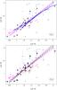 |
Fig. 5 Comparison of electron temperatures te(O iii) (te = 10-4 Te) obtained from [O iii]λ4363/(λ4959 + λ5007) and te(S iii) obtained from [S iii]λ6312/λ9069 emission-line ratios. VLT/UVES data are shown by stars, except for three objects with uncertain values, which are shown as open circles (see Sect. 3.1). Twenty-seven data points from SDSS DR3 (see text) are shown by red dots. Open blue diamonds, blue asterisks, and purple triangles correspond to data from Kehrig et al. (2006), Pérez-Montero & Diaz (2003) and García-Rojas & Esteban (2007), respectively. The dashed blue line in the upper panel connects locations of equal temperature. The thick blue lines (also in the upper panel) are the predicted te(S iii) – te(O iii) relations for H ii region models from Izotov et al. (2006). The dotted and thin solid black lines are the curves from Garnett (1992) and Pérez-Montero & Diaz (2005), respectively. Regression lines (solid lines) and 1σ alternatives (dashed lines) for all our data plus data from García-Rojas & Esteban (2007) are shown by purple lines. In the lower panel the error bars are shown for the VLT, SDSS, and García-Rojas & Esteban (2007) data. Additionally, regression lines for VLT+SDSS-only data are shown by black lines. (A color version of this figure is available in the online journal.) |
3. Physical conditions in the H II regions
Physical conditions and element abundances in the selected H ii regions were derived with the atomic data from the references listed in Stasińska (2005).
3.1. Electron temperatures
Nineteen out of the thirty one H ii regions observed with VLT/UVES (Table 3) have detectable [S iii]λ6312 and [S iii] λ9069 emission lines in their spectra. This gives us the opportunity to determine the electron temperature Te(S iii) directly from the spectra. In Fig. 5 we compare the electron temperatures te(O iii) and te(S iii) (te = 10-4Te) obtained from [O iii]λ4363/(λ4959+λ5007) and [S iii]λ6312/λ9069, respectively. The H ii region data from VLT/UVES, including those for SBS 0335–052E from Izotov et al. (2009), are shown by stars. An exception are the three galaxies, which are represented by open circles. One of them (bottom left corner in both panels) belongs to the galaxy He 2–10E (UVES, ESO program 081.C-0113(A)). Its spectrum is noisy with a very weak and uncertain [O iii]λ4363 line intensity. The other two, in the upper right corner, belong to Tol 1214–277 (UVES, ESO program 69.D-0174(A)) and UM 133H (UVES, ESO program 68.B-0310(A)). At the redshift of Tol 1214–277 two absorption night-sky lines (λ9300.6 and λ9303.9) coincide with the brightest part of the profile of the [S iii]λ9069 emission line, reducing its flux by ~20% so that te(S iii) is overestimated (the point is actually outside the figure, which is indicated by an arrow). In UM133, the [S iii]λ9069 emission line is affected by the night sky line at λ9118. All our VLT/UVES and FORS data shown in Figs. 5−11 are presented in Table 10.
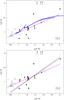 |
Fig. 6 Comparison of electron temperatures te(O iii) (te = 10-4 Te) obtained from [O iii]λ4363/(λ4959 + λ5007) and te(N ii) obtained from [N ii]λ5755/λ6583 emission-line ratios. VLT/UVES and FORS data are shown by stars, except for two objects, which are shown as open circles (see text). Green asterisks and open purple triangles provide the data from Esteban et al. (2009) and García-Rojas & Esteban (2007), respectively. The thick blue lines show the predicted te(O ii) – te(O iii) relation for H ii region models from Izotov et al. (2006). Regression lines (solid lines) and 1σ alternatives (dashed lines) for all data are shown by purple lines. The lower panel shows the error bars. Additionally, regression lines for our VLT-only data are shown by black lines. (A color version of this figure is available in the online journal.) |
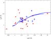 |
Fig. 7 Comparison of electron temperatures te(O iii) (te = 10-4 Te) derived from [O iii]λ4363/(λ4959 + λ5007) and te(O ii) obtained from [O ii]λ3727/(λ7320 + λ7330) emission-line ratios. VLT/UVES and FORS data are shown by red stars and blue filled circles, respectively. The thick blue lines represent the te(O ii) – te(O iii) relations from Izotov et al. (2006). (A color version of this figure is available in the online journal.) |
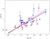 |
Fig. 8 Comparison of electron temperatures te(O iii) (te = 10-4 Te) obtained from [O iii]λ4363/(λ4959 + λ5007) and te(S ii) obtained from [S ii]λ4068/(λ6717 + λ6730) emission-line ratios. Symbols are the same as in Fig. 7. Regression lines for all data are represented by purple lines. Regression lines for the UVES-only data are shown by black lines. (A color version of this figure is available in the online journal.) |
Additionally, we plot as red dots the data from Izotov et al. (2006) for the SDSS DR3. Out of more than ~300 emission-line galaxies selected from the SDSS DR3 because they have a detectable [O iii]λ4363 line, we show here only the 27 galaxies for which F(Hβ) is higher than 2 × 10-14 erg s-1 cm-2 and for which the errors in the [O iii]λ4363 fluxes are lower than 25%. For comparison we also show data from Kehrig et al. (2006) (open blue rombs), Pérez-Montero & Diaz (2003) (blue asterisks) and García-Rojas & Esteban (2007) (purple triangles). The data by Pérez-Montero & Diaz (2003) and Kehrig et al. (2006) were obtained from a spectroscopic analysis of H ii regions in emission-line galaxies with ongoing star formation and the data by García-Rojas & Esteban (2007) were derived for H ii regions in our Galaxy.
The dashed blue line in the top panel connects points of equal temperatures. The thick
lines show the predicted te(S iii) –
te(O iii) relation for H ii region
sequences of photoionization models with low, intermediate, and high metallicities
(12 + log O/H = 7.2, 7.6 and 8.2) from Izotov et al.
(2006). The dotted and solid black lines display the model prediction from Garnett (1992) and Pérez-Montero & Diaz (2005), respectively. The regression line including our
data, the SDSS data, and the data from García-Rojas &
Esteban (2007) are shown by purple lines. Its equation is  (2)The regression was computed using the maximum
likelihood method by Press et al. (1992) that
includes error bars on both axes. In the lower panel the error bars concerning the VLT,
SDSS, García-Rojas & Esteban (2007) data and
additional regression lines for VLT and SDSS-only data are shown by black lines.
(2)The regression was computed using the maximum
likelihood method by Press et al. (1992) that
includes error bars on both axes. In the lower panel the error bars concerning the VLT,
SDSS, García-Rojas & Esteban (2007) data and
additional regression lines for VLT and SDSS-only data are shown by black lines.
Clearly the data presented here define a much better empirical relation between te(S iii) and te(O iii) than previous work on extragalactic H ii regions. We note that the VLT/UVES data follow the same distribution as the best data from SDSS DR3. Unfortunately, for high electron temperatures there are only few data with reliable temperature determinations.
In metal-poor galaxies, [N ii]λ5755 is extremely weak. Only in 19 out of 121 VLT spectra could it be measured. To enlarge the range of temperatures we also added VLT/FORS data for the hot H ii region in J0519+0007 from Guseva et al. (2009). In Fig. 6 we plot te(N ii) obtained from [N ii]λ5755/λ6583 as a function of te(O iii). Data from our VLT sample are represented by stars. Tol 2240-384 (FORS medium and low resolution) and Tol 2138-405 No.3 (FORS medium resolution) are denoted by open circles with arrows, indicating that they are outside the plot owing to large te(N ii). Green asterisks display the data from Esteban et al. (2009). By open purple triangles we show the data from García-Rojas & Esteban (2007).
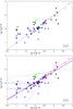 |
Fig. 9 Ne(O ii) versus Ne(S ii). Black stars: VLT-UVES; filled blue circles: FORS observations (medium resolution). Purple triangles: data from García-Rojas & Esteban (2007), green asterisks: data from Esteban et al. (2009). The dashed blue line connects points of equal densities. The lower panel shows the error bars and regression lines and their 1σ alternatives for all data (purple lines) and for the VLT-only data (black lines). (A color version of this figure is available in the online journal.) |
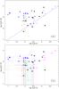 |
Fig. 10 Ne(Cl iii) versus Ne(S ii). UVES, FORS and SDSS DR3 data are represented by black stars, filled blue circles, and red dots, respectively. Purple triangles: data from García-Rojas & Esteban (2007), green asterisks: data from Esteban et al. (2009). The dashed blue line connects points of equal densities. The lower panel shows the error bars. (A color version of this figure is available in the online journal.) |
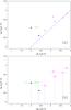 |
Fig. 11 Ne(Ar iv) versus Ne(S ii). FORS data are represented by filled blue circles. Purple triangles: data from García-Rojas & Esteban (2007), green asterisks: data from Esteban et al. (2009). The dashed blue line connects points of equal densities. The lower panel shows the error bars. (A color version of this figure is available in the online journal.) |
The thick blue lines in the top panel of Fig. 6 represent the te(O ii) – te(O iii) relation from the same Izotov et al. (2006) models as those considered in Fig. 5. It roughly follows the observational points, which show a substantial scatter. However, at the lowest temperatures considered, there seems to be an offset between the blue lines and our observational points.
The regression line for all data (upper panel) is given by the equation:  (3)The lower panel shows the error bars.
Additionally, regression lines for our VLT-only data are shown by black lines.The electron
temperature derived from [S iii]λ6312/λ9069 or
[N ii]λ5755/λ6583 allowed us to obtain an
empirical relation between those temperatures and the one derived from
[O iii]λ4363/λ(4959+5007) for the first time
for metal-poor galaxies.
(3)The lower panel shows the error bars.
Additionally, regression lines for our VLT-only data are shown by black lines.The electron
temperature derived from [S iii]λ6312/λ9069 or
[N ii]λ5755/λ6583 allowed us to obtain an
empirical relation between those temperatures and the one derived from
[O iii]λ4363/λ(4959+5007) for the first time
for metal-poor galaxies.
In 21 UVES and 16 FORS spectra [O ii]λ3727 and
λλ7320,7330 lines have been measured. The [S
ii]λ4068 and λλ6717,6730
lines are detected and measured in 24 UVES and 27 FORS spectra. These allow us to derive
the electron temperatures te(O ii) and
te(S ii) by direct methods. The results are shown
in Figs. 7 and 8, where we compare those values with te(O
iii). The UVES data are shown by red stars. Blue filled circles correspond to
FORS data. The thick blue lines in Fig. 7 represent
the te(O ii) – te(O
iii) relations from Izotov et al.
(2006). Despite the large spread of points in Fig. 7 the VLT/UVES and FORS data follow the predicted
te(O ii) – te(O
iii) relations (Izotov et al. 2006). The
values of te(S ii) in Fig. 8 correlate well with te(O iii),
but are significantly below te(O ii) in Fig. 7. Regression lines for all data in Fig. 8 are shown by purple lines and for the UVES-only data by
black lines. The regression line for all the data displayed in Fig. 8 is given by the equation:  (4)
(4)
3.2. The electron number densities
For all galaxies the electron number densities Ne(S ii) were obtained from the [S ii] λ6717/λ6731 emission line ratio, except for regions where these emission lines are too weak to allow density determinations. For abundance determinations in those regions we adopt Ne = 10 cm-3. The value of the electron number densities does not significantly affect the derived abundances in the low-density limit, which holds for the bulk of the H ii regions considered here. The electron number densities Ne(S ii) derived from the [S ii] λ6717/λ6731 emission line ratio are given in Tables 6, 7 and 8.
The high signal-to-noise ratio and high spectral resolution of the spectra in the VLT sample allow us to measure the fluxes of the weak emission lines [Ar iv]λ4711, 4740 and [Cl iii]λ5517, 5537 and to separate and measure the fluxes of the [O ii]λ3726,3729 lines to determine the electron number density. In many UVES spectra [O ii]λ3726 and [O ii]λ3729 are seen as separate lines (for instance in UM 254, Fig. 2). However, for H ii regions with broad components in their emission lines these two lines are poorly separated. In those cases the IRAF routine SPLOT was used for deblending. For all FORS medium resolution data the [O ii] λ3726+3729 lines were deblended by this IRAF software routine, adopting preliminary estimated widths of each of these emission lines.
The top panel of Fig. 9 shows Ne(O ii) versus Ne(S ii). The data from UVES observations are shown by black stars, whereas medium-resolution FORS data are denoted by filled blue circles. We did not include SDSS data because of the very large errors in Ne(O ii) determinations. Purple triangles represent data from García-Rojas & Esteban (2007), green asterisks data from Esteban et al. (2009). The dashed blue line connects points of equal densities. The bottom panel of Fig. 9 shows the same data as the upper panel, but with error bars and regression lines.
The regression line for all data shown in Fig. 9
(lower panel, purple line) is presented by the equation ![Mathematical equation: \begin{eqnarray} \log {N}_{\rm e}({\rm O II}) &=& (0.3413\pm1.2484) + (0.8782\pm0.4798) \nonumber\\[1.5mm] \label{neOII}&& \times \log{N}_{\rm e}({\rm S II}). \end{eqnarray}](/articles/aa/full_html/2011/05/aa16291-10/aa16291-10-eq32.png) (5)The top panel of Fig. 10 shows Ne(Cl iii) versus
Ne(S ii). UVES, FORS and SDSS DR3 data are
represented by black stars, filled blue circles and red dots, respectively. Purple
triangles are the data from García-Rojas & Esteban
(2007), green asterisks are the data from Esteban
et al. (2009). The dashed blue line displays locations with equal densities. The
error bars are shown in the lower panel. Only 14 SDSS galaxies could be used to derive
Ne(Cl iii) due to our requirement that the error of
the [Cl iii]λ5517 emission line flux is less than 25%. Five of
them are shown by red dots. For the remaining nine, the SDSS data allow only the
derivation of a lower limit of 10 cm-3 (they are not shown in the figure).
(5)The top panel of Fig. 10 shows Ne(Cl iii) versus
Ne(S ii). UVES, FORS and SDSS DR3 data are
represented by black stars, filled blue circles and red dots, respectively. Purple
triangles are the data from García-Rojas & Esteban
(2007), green asterisks are the data from Esteban
et al. (2009). The dashed blue line displays locations with equal densities. The
error bars are shown in the lower panel. Only 14 SDSS galaxies could be used to derive
Ne(Cl iii) due to our requirement that the error of
the [Cl iii]λ5517 emission line flux is less than 25%. Five of
them are shown by red dots. For the remaining nine, the SDSS data allow only the
derivation of a lower limit of 10 cm-3 (they are not shown in the figure).
The top panel of Fig. 11 shows Ne(Ar iv) versus Ne(S ii). The FORS data are represented by filled blue circles. Purple triangles are the data from García-Rojas & Esteban (2007), green asterisks are the data from Esteban et al. (2009). The dashed blue line is the place of equal densities. The lower panel shows the error bars and regression lines for all data. For Ne(Ar iv), we have a proper estimate for only two H ii regions and a lower limit of 10 cm-3 for 50 H ii regions (not shown in the figure).
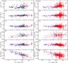 |
Fig. 12 log N/O a), log Ne/O b), log S/O c), log Cl/O d), log Ar/O e) and log Fe/O f) vs. oxygen abundance 12 + log O/H for our sample of 121 spectra (large stars). Several knots in H ii regions NGC 346 and NGC 456 in the SMC are shown by green and purple large asterisks, respectively. Additionally we show the galaxies from the HeBCD sample of Izotov et al. (2004) and Izotov & Thuan (2004) for the primordial He abundance determination (small filled blue circles) and the sample of ~300 emission-line galaxies from the SDSS DR3 (Izotov et al. 2006) (red dots). The solar abundance ratios by Lodders (2003) and by Asplund et al. (2009) are indicated by the purple and black large open circles and the associated error bars. The straight black lines are linear regressions for the HeBCD sample by Izotov et al. (2006) and the purple ones are for all (except the SDSS data). The right panel shows the error bars. (A color version of this figure is available in the online journal.) |
For all the objects Ne(O ii) is very similar to Ne(S ii) in the whole density range. Note that H ii regions with Ne(S ii) larger than 200 cm-3 represent only ~10% of the entire VLT sample (Tables 6−8). On the other hand, Ne(Cl iii) and Ne(Ar iv) are systematically higher than Ne(S ii). This has no consequence on our determination of heavy element abundances below, but it will be important for considering the derivation of the pregalactic helium abundance.
4. Element abundances
4.1. Derivation of the abundances
The above analysis shows that the relations te(S iii) vs. te(O iii), te(N ii) and te(O ii) vs. te(O iii) derived from observations follow the same trends as the models by Izotov et al. (2006). Because the observed values are affected by large uncertainties in some cases and because many spectra lack the necessary data for the determination of te(S iii) and te(N ii), we prefer to use the same prescriptions as in Izotov et al. (2006).
To derive the abundances of O2+, Ne2+ and Ar3+, we adopted the temperature Te(O iii) directly derived from the [O iii] λ4363/(λ4959 + λ5007) emission-line ratio.
For O+, N+, S+, and Fe2+, we took the value
of te(O ii) obtained from
te(O iii) using Eq. (14) in Izotov et al. (2006) that is shown below: ![Mathematical equation: \begin{eqnarray} t_{\rm e}({\rm O\ II}) &=& -0.577+t_{\rm e}({\rm O\ III})\times\left[2.065-0.498t_{\rm e}({\rm O\ III})\right], \nonumber\\ t_{\rm e}({\rm O\ II}) &=& -0.744+t_{\rm e}({\rm O\ III})\times\left[2.338-0.610t_{\rm e}({\rm O\ III})\right], \nonumber\\ \label{toii}t_{\rm e}({\rm O\ II}) &=& 2.967+t_{\rm e}({\rm O\ III})\times\left[-4.797+2.827t_{\rm e}({\rm O\ III})\right], \end{eqnarray}](/articles/aa/full_html/2011/05/aa16291-10/aa16291-10-eq37.png) (6)for 12 + log O/H = 7.2 and
te(O iii) ≥ 1.14, 12 + log O/H = 7.6 and
te(O iii) ≥ 1.14 and 12 + log O/H = 8.2 and
te(O iii) ≤ 1.18, respectively (see thick blue
lines in Fig. 6a).
(6)for 12 + log O/H = 7.2 and
te(O iii) ≥ 1.14, 12 + log O/H = 7.6 and
te(O iii) ≥ 1.14 and 12 + log O/H = 8.2 and
te(O iii) ≤ 1.18, respectively (see thick blue
lines in Fig. 6a).
Similarly, to compute the S2+, Cl2+, and Ar2+ abundances
we adopted the value of te(S iii) obtained from
te(O iii) using Eq. (15) in Izotov et al. (2006): ![Mathematical equation: \begin{eqnarray} t_{\rm e}({\rm S\ III}) &=& -1.085+t_{\rm e}({\rm O\ III})\times\left[2.320-0.420t_{\rm e}({\rm O\ III})\right], \nonumber\\ t_{\rm e}({\rm S\ III}) &=& -1.276+t_{\rm e}({\rm O\ III})\times\left[2.645-0.546t_{\rm e}({\rm O\ III})\right], \nonumber\\ \label{tsiii}t_{\rm e}({\rm S\ III}) &=& 1.653+t_{\rm e}({\rm O\ III})\times\left[-2.261+1.605t_{\rm e}({\rm O\ III})\right], \end{eqnarray}](/articles/aa/full_html/2011/05/aa16291-10/aa16291-10-eq43.png) (7)for 12 + log O/H = 7.2 and
te(O iii) ≥ 1.14, 12 + log O/H = 7.6 and
te(O iii) ≥ 1.14 and 12 + log O/H = 8.2 and
te(O iii) ≤ 1.18, respectively (see thick blue
lines in Fig. 5a).
(7)for 12 + log O/H = 7.2 and
te(O iii) ≥ 1.14, 12 + log O/H = 7.6 and
te(O iii) ≥ 1.14 and 12 + log O/H = 8.2 and
te(O iii) ≤ 1.18, respectively (see thick blue
lines in Fig. 5a).
Equations (6) and (7) (identical with Eqs. (14) and (15) in Izotov et al. 2006) are based on the H ii region-photoionization models calculated for the given restricted (though large) ranges of input parameters and with the stellar atmosphere models by Smith et al. (2002) for the three values of the metallicity corresponding to 12 + log O/H = 7.2, 7.6 and 8.2 (see thick blue lines in Figs. 6a and 5a). Therefore they hold for the restricted ranges of 12 + log O/H and te(O iii) and we did not extrapolate them outside these ranges. The electron temperatures te(O ii) and te(S iii) depend on both the oxygen abundance 12 + log O/H and the electron temperature te(O iii). To derive these we fixed te(O iii) and iteratively obtained 12 + log O/H and te(O ii). First, the approximate value of te(O ii) was derived from the first expression of Eq. (6) if te(O iii) ≥ 1.14 or from the third expression of Eq. (6) if te(O iii) < 1.14. Then the oxygen abundance was derived. Given the new iterative value of 12 + log O/H, the new value of te(O ii) was obtained. This process was continued until the convergence of both 12 + log O/H and te(O ii) was achieved.
After that te(S iii) was derived. We used the linear interpolation of te(O ii) and te(S iii) between 12 + log O/H = 7.2, 7.6 and 8.2 to the iterative value of 12 + log O/H. The interpolation ranges for 12 + log O/H are between 7.2 and 8.2 for the te(O iii) range between 1.14 and 1.18 and are between 7.2 and 7.6 for te(O iii) > 1.18. If the electron temperature te(O iii) < 1.14, we adopted the equations for 12 + log O/H = 8.2 to derive te(O ii) and te(S iii) (see Fig. 6a). If the iterated oxygen abundance was above the 12 + log O/H = 8.2, we used the third lines in Eqs. (6) and (7) for the determination of te(O ii) and te(S iii). If the iterated 12 + log O/H < 7.2 we used the first lines in Eqs. (6) and (7) for the determination of te(O ii) and te(S iii).
The electron temperatures Te(O iii), Te(O ii), Te(S iii) and electron number density Ne(S ii) are given in Table 6 (UVES observations) and Tables 7 and 8 (low- and medium-resolution FORS observations).
All the ionic abundances were computed using the low-density limit of the emissivities.
In all H ii regions the abundances of O+ and O2+ were obtained from the fluxes of the [O ii] λ3727 and [O iii]λ4959, 5007 lines, respectively. We added the small fraction of the undetected O3+ ion to the oxygen abundance in high-excitation H ii regions with O+/(O++O2+) ≤ 0.1 if the He ii λ4686 emission line was detected in their spectra. The total elemental abundances of the other elements were derived using the empirical ionization correction factors (ICFs) of Izotov et al. (2006, their Eqs. (18)−(24)). Similar to the electron temperatures, we used the linear interpolation of ICFs in the oxygen abundance range 12 + log O/H = 7.2−8.2 given the derived oxygen abundance for a particular H ii region. If the oxygen abundance of the H ii region was greater than 8.2, we adopted ICFs for 12 + log O/H = 8.2. Conversely, if the oxygen abundance of the H ii region was less than 7.2 we adopted ICFs for 12 + log O/H = 7.2. The ionic and total O, N, Ne, S, Cl, Ar, and Fe abundances derived from the forbidden emission lines are given in Tables 6−8 for the UVES and FORS observations. The quoted errors in the element abundances account for the uncertainties in the ionization correction factors.
4.2. Abundance patterns from collisionally excited lines (CELs)
The derived oxygen abundances for our VLT sample are found to cover the range of 12 + log O/H ~ 7.2−8.4. In Fig. 12 left panel, we show the abundance ratios versus metallicities for the 121 spectra from our VLT sample (large stars). Several knots in H ii regions NGC 346 and NGC 456 in the SMC are shown by green and purple large asterisks, respectively. We also plot the data from the HeBCD sample collected by Izotov et al. (2004) and Izotov & Thuan (2004) (filled blue circles) and those from the DR3 of SDSS (Izotov et al. 2006) (red dots). The HeBCD sample possesses more than 100 high-quality spectra of low-metallicity galaxies for the primordial He abundance determination. The error bars are shown in the right panel of the figure.
In each panel, the solar abundance ratio by Lodders (2003) is indicated by the purple large open circle along with the associated error bar, whereas the solar abundance ratio by Asplund et al. (2009) is indicated by the black large open circle. The straight black and purple lines in Fig. 12 are the linear regressions obtained for the HeBCD sample taken from the paper by Izotov et al. (2006) and for all data (121 VLT + 109 HeBCD spectra) respectively. The SDSS data have larger errors (Fig. 12, right panel) and therefore are not included in the regressions.
The regression lines for all data (excluding SDSS) are given by the equations
![Mathematical equation: \begin{eqnarray} &&{\rm Ne}/{\rm O} = [(-1.2850\pm0.0472) + (0.0656\pm0.0059)]\times X,\nonumber\\[1.5mm] &&\qquad\qquad \qquad\qquad \qquad\qquad(n = 249, \chi^2 = 1141), \label{Ne/O}\\[1.5mm] &&{\rm S}/{\rm O} = [(-1.8310\pm0.0532)+(0.0244\pm0.0066)] \times X,\nonumber\\[1.5mm] &&\qquad\qquad \qquad\qquad \qquad\qquad(n = 203, \chi^2 = 6126), \label{S/O}\\[1.5mm] &&{\rm Cl}/{\rm O} = [(-5.7188\pm0.0933)+(0.2680\pm0.0115)] \times X,\nonumber\\[1.5mm] &&\qquad\qquad \qquad\qquad \qquad\qquad (n = 98, \chi^2 = 1701), \label{Cl/O}\\[1.5mm] &&{\rm Ar}/{\rm O} = [(-2.1739\pm0.0586)+(-0.0221\pm0.0071)] \times X,\nonumber\\[1.5mm] &&\qquad\qquad \qquad\qquad \qquad\qquad (n = 196, \chi^2 = 5146), \label{Ar/O}\\[1.5mm] &&{\rm Fe}/{\rm O} = [(5.7180\pm0.0998) + (-0.9452\pm0.0121)] \times X,\nonumber\\[1.5mm] \label{Fe/O}&&\qquad\qquad \qquad\qquad \qquad\qquad (n = 165, \chi^2 = 9032), \end{eqnarray}](/articles/aa/full_html/2011/05/aa16291-10/aa16291-10-eq179.png) where X = 12 + log O/H.
where X = 12 + log O/H.
Overall, we see in Fig. 12 a good overlap of our present VLT sample with the HeBCD and SDSS DR3 samples. The S/O, Cl/O and Ar/O abundance ratios are close to the distributions previously obtained by Izotov et al. (2006) and do not show any significant trend with oxygen abundance. Similar distributions for S/O and Ar/O have been obtained by Thuan et al. (1995), Izotov & Thuan (1999) and van Zee & Haynes (2006). We confirm the previous results using a significantly larger data base that encompasses 230 high-quality data. Some slight trends in S/O, Cl/O and Ar/O abundance ratios could imply a metallicity dependence of the α-element production by massive stars. Variations of the explosion energy of Type II supernovae with low metallicity might also play a role (Kobayashi et al. 2006). However, Izotov et al. (2006) pointed out that abundance determinations for some elements such as S, Cl, and Ar could be uncertain because of the uncertainties in atomic data, e.g., in the rates of dielectronic recombination.
The ratio Ne/O (Fig. 12b) shows a slight increase with increasing 12 + log O/H. This is likely explained by a stronger depletion of oxygen onto dust grains in higher-metallicity galaxies.
The most prominent trend was found by Izotov et al. (2006) for the Fe/O abundance ratio, which decreases with increasing O/H. While its value is nearly solar at the lowest metallicities, it drops by one order of magnitude at 12 + log O/H = 8.5. The interpretation of this trend put forward by Izotov et al. (2006) is that it is due to depletion of Fe onto dust grains, which becomes more important at higher metallicities.
The behavior of the N/O ratio is particularly interesting. Izotov & Thuan (1999) and Izotov et al. (2006) have demonstrated that the dispersion in N/O in low-metallicity BCDs with 12 + log O/H < 7.5−7.6 is very low with a plateau value of log N/O ~−1.6. However, in a larger sample (Fig. 12a) some galaxies have a higher N/O ratio at 12 + log O/H < 7.6. Several points with highest N/O at 12 + log O/H ~ 7.5 (Fig. 12a) belong to galaxies with low EW(Hβ) (10 to 70 Å). The notable exception is J0519+0007 with EW(Hβ) = 240 Å. This is in line with the finding of Izotov et al. (2006) that the observed N/O increases as EW(Hβ) decreases. They showed that this enhancement could be due to high-density nitrogen-rich ejecta from massive stars during W-R phases. The fact that no W-R features are detected in these HII regions is not a counterargument, because the W-R phase is expected to be short and the W-R features are weak in these low-metallicity systems.
We also find that the lower limit of N/O in H ii regions with lowest metallicity is higher than the above-mentioned plateau value of −1.6, implying that there is some increase in N/O with decreasing oxygen abundance at 12 + log O/H < 7.5 (Fig. 12a). If true, this tendency would agree with the prediction of primary nitrogen being produced by low-metallicity rotating stars, as found by Meynet & Maeder (2002). Although these authors considered stellar models with a heavy element mass fraction Z = 10-5, which is significantly lower than the values of Z ~ 0.0002−0.0005 in the lowest-metallicity H ii regions analyzed by us, it is possible that the interstellar medium in these galaxies enriched by the first metal-free stars memorizes this.
The two H ii regions in the SMC considered by us, NGC 346 and NGC 456, have very low values of log Fe/O, extending from −1.5 down to −2.6. It would be interesting to investigate why these H ii regions show such an extreme behavior. The remaining elements (Ne, S, Cl, Ar) follow the same trends as in the other H ii regions, with the exception of N/O. NGC 346 and NGC 456 have the lowest N/O ratio among all the H ii regions in our sample.
4.3. Ionic abundances from recombination lines
We detected and measured the fluxes of the recombination lines (RLs) O ii λ4650 and C ii λ4267 in eight medium-resolution FORS (out of 30) and 17 UVES (out of 31) H ii region spectra. We detected only two out of eight O ii recombination lines of multiplet 1. The multiplet consists of eight lines: λ4639, λ4642, λ4649, λ4651, λ4662, λ4674, λ4676, and λ4696. It is rarely possible to measure all the lines of this multiplet, and frequently it is necessary to estimate the intensities of the unobserved or blended lines. Owing to the insufficient resolution of the FORS medium resolution spectra, the O ii λ4649 and O ii λ4651 lines are blended into the pair 4649+4651 named O ii λ4650. In the UVES spectra we measured the O iiλ4649 and λ4651 lines separately, which were then co-added and named O ii λ4650. The intensities of O ii λ4650 and C ii λ4267 lines were corrected for reddening using the extinction coefficient C(Hβ) from Tables 3 and 5. Following Esteban et al. (2009) we calculated the abundance of O++/H+ from O ii λ(4649+4651) and of C++/H+ from C ii λ4267. For the determination of the O++ abundances we used the prescriptions by Peimbert et al. (2005) to calculate the correction factor for the contribution of unmeasured lines of multiplet 1 for the non-LTE conditions. The intensities of the lines of multiplet 1 weakly depend on the electron density. We used the values of Ne(S ii) to derive the correction factors. If taking a higher value of the density, as indicated by Ne(Cl iii) (Fig. 10) and Ne(Ar iv) (Fig. 11), the RL abundances decrease by ~5−15%. The effective recombination coefficients were taken from Storey (1994) for O ii RLs and from Davey et al. (2000) for C ii RLs.
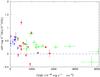 |
Fig. 13 Comparison of the abundance discrepancy factor ADF = log O++(RL)/O++(CEL) with observed F(Hβ). Data from UVES and FORS medium resolution observations are shown by red stars and filled blue circles. Green asterisks are the data from Esteban et al. (2009). (A color version of this figure is available in the online journal.) |
In Table 9 we present the observed fluxes of O ii λ4650, C ii λ4267 and Hβ emission lines, the ionic abundances of O++/H+ obtained from RLs and CELs, and C++/H+ obtained from RLs using the electron temperature derived from [O iii] λ4363/(λ4959 + λ5007).
O++ is the only ion for which both strong CELs and measured RLs are present in the optical range. In Fig. 13 we show the dependence of the abundance discrepancy factor ADF = log O + + (RL)/O++(CEL) on the observed F(Hβ). UVES data are shown by red stars, FORS medium-resolution data by filled blue circles. We determined, where possible, ADF and C++(RL) and compared our results with those of other studies. Green asterisks represent the data from Esteban et al. (2009). There is no clear trend with F(Hβ) for F(Hβ) > 10-13 erg s-1 cm-2 and the error bars are large. Many UVES cases are compatible with no discrepancy at all. However, half of the cases, especially the FORS and UVES data with F(Hβ) < 10-13 erg s-1 cm-2, indicate an ADF clearly larger than zero. This is in line with what was found by Esteban et al. (2009) for a set of extragalactic H ii regions as well with what is summarized by García-Rojas & Esteban (2007) for galactic H ii regions. We investigated the possible existence of a correlation between the ADF and any of the following parameters: C(Hβ), O+/(O++O+), O/H (CEL), FWHM(Hβ) and electron number density, hoping to find a clue for the origin of those ADFs. Like García-Rojas & Esteban (2007), we found no evidence for any correlation whatsoever.
Whatever the reason for the abundance discrepancy may be, we can use the C++(RL)/O++(RL) ratio to achieve some insight into the behavior of the C/O ratio. Figure 14 shows the values of log C++(RL)/O++(RL) as a function of 12 + log O/H(CEL). The symbols are the same as in Fig. 13. We supplement our data with those from Garnett et al. (1995), where C++/O++ are derived from the UV CELs and García-Rojas & Esteban (2007), which are shown by filled and open purple triangles, respectively. Green asterisks are the data from Esteban et al. (2009). The data from Garnett et al. (1999) and Kobulnicky & Skillman (1998) for the C iii]1909 line are shown by light blue squares and black circles, respectively. We find that if C++(RL)/O++(RL) can be taken as a measure of C/O, the C/O ratio increases with O/H. The only objects that do not follow this trend are the ones from our sample and from Esteban et al. (2009) and Kobulnicky & Skillman (1998), for which only 1σ upper limits to the C ii λ4267 line flux are estimated. The two leftmost points are for Tol 1214−277. One of these points is from the UVES spectrum, where only upper limits to the F(O ii) and F(C ii) are obtained, and the second point is from the FORS medium-resolution spectrum. Four points at 12 + log O/H ~ 8.05 belong to NGC 6822 V No. 1 and to three knots in the SMC H ii region NGC 346. Note, that for NGC 346 no night sky subtraction was made.
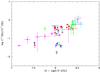 |
Fig. 14 Dependence of the ion abundance ratio log C++(RL)/O++(RL) on 12 + log O/H(CEL). Our data are marked by the same symbols as in Fig. 13. Data from Garnett et al. (1995) and García-Rojas & Esteban (2007) are shown by filled and open purple triangles, respectively. Green asterisks are the data from Esteban et al. (2009). Data from Garnett et al. (1999) and Kobulnicky & Skillman (1998) are shown by light blue squares and black circles, respectively. (A color version of this figure is available in the online journal.) |
5. Summary
We have presented an analysis of archival VLT/FORS1+UVES spectroscopic observations of a large sample of low-metallicity emission-line galaxies. The whole sample, which contains some data from our previous papers (Izotov et al. 2009; and Guseva et al. 2009), consists of 121 spectra, out of which 83 are analyzed for the first time. For comparison, we also used data from SDSS DR3 studied by Izotov et al. (2006) and 109 spectra from the HeBCD sample observed with different telescopes and collected by Izotov & Thuan (2004) and Izotov et al. (2004) for the study of the primordial He abundance.
Our main results are as follows:
-
1.
The oxygen abundance in the sample lies in the range 12 + log O/H = 7.2−8.4. The abundance ratios of the α-elements to oxygen follow the trends found in our previous studies of low-metallicity emission-line galaxies. In particular, the new data confirm with a larger sample of 230 H ii regions the finding by Izotov et al. (2006) that Ne/O increases with increasing oxygen abundance, which is interpreted as caused by a higher depletion of oxygen in higher-metallicity galaxies. The S/O, Cl/O and Ar/O abundance ratios are close to the distributions obtained previously by Izotov et al. (2006). Slight trends seen in S/O, Cl/O and Ar/O abundance ratios could imply a metallicity dependence of the α-element production by massive stars. Variations of the explosion energy of Type II supernovae with metallicity might also play a role (Kobayashi et al. 2006). However, as already pointed out by Izotov et al. (2006), the abundance determinations of these elements may suffer from uncertainties owing to inaccurate ionization correction factors.
-
2.
The Fe/O ratio shows an underabundance of iron relative to oxygen as compared to the solar value, which is particularly large for the high-metallicity galaxies. This again confirms the finding by Izotov et al. (2006) and strengthens our interpretation that Fe is depleted onto dust grains and that this effect depends on the metallicity.
-
3.
There is a tendency for N/O to increase with decreasing oxygen abundance in extremely low-metallicity galaxies with 12 + log O/H < 7.5. This could be a sign of enhanced production of primary nitrogen by rapidly rotating metal-free stars (Meynet & Maeder 2002).
-
4.
The electron temperature derived from [S iii]λ6312/λ9069 or [N ii]λ5755/λ6583 in a number of objects allowed us to obtain for the first time in metal-poor galaxies an empirical relation between those temperatures and the one derived from [O iii]λ4363/λ(4959+5007). We also present the empirical relation between te derived from [O ii]λ3727/(λ7320 + λ7330) or [S ii]λ4068/(λ6717 + λ6730) and [O iii]λ4363/λ(4959+5007).
-
5.
The electron number densities Ne(O ii), Ne(Cl iii), Ne(Ar iv) could be obtained for a number of objects in addition to Ne(S ii). We find that Ne(O ii) is very similar to Ne(S ii), while Ne(Cl iii) and Ne(Ar iv) are systematically higher. This has potential implications when deriving the pregalactic helium abundance, since the He I lines are predominantly emitted in those higher density zones.
-
6.
In a number of objects, the abundances of C++ and O++ could be derived from recombination lines (RLs). We find that O++ abundances obtained from RLs tend to be higher than those derived from collisionally excited lines (CELs), as found in previous studies of galactic and a few extragalactic H ii regions. In the C++/O++ vs. O/H diagram, most of the new points follow the relation obtained by previous observations of C/O increasing with O/H.
Online material
Spectroscopic properties of H ii regions.
Extinction-corrected emission line fluxes (UVES observations).
Extinction-corrected emission line fluxes (low-resolution FORS observations).
Extinction-corrected emission line fluxes (medium-resolution FORS observations).
Ionic and total heavy element abundances (UVES observations).
Ionic and total heavy element abundances (FORS low-resolution observations).
Ionic and total heavy element abundances (FORS medium-resolution observations).
Recombination lines: fluxes and ionic abundances.
Electron temperatures and electron number densities derived from emission line flux ratios.
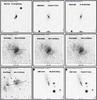 |
Fig. 1 Optical images of the galaxies. The straight lines indicate the location of the slit during observations (see Table 1). |
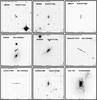 |
Fig. 1 continued. |
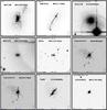 |
Fig. 1 continued. |
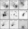 |
Fig. 1 continued. |
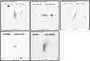 |
Fig. 1 continued. |
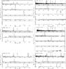 |
Fig. 2 Flux-calibrated and redshift-corrected UVES spectra of galaxies. |
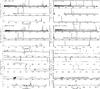 |
Fig. 2 continued. |
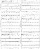 |
Fig. 2 continued. |
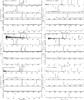 |
Fig. 2 continued. |
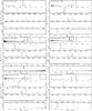 |
Fig. 2 continued. |
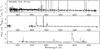 |
Fig. 2 continued. |
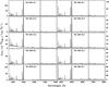 |
Fig. 3 Flux-calibrated and redshift-corrected FORS low-resolution spectra of galaxies. |
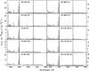 |
Fig. 3 continued. |
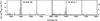 |
Fig. 3 continued. |
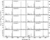 |
Fig. 4 Flux-calibrated and redshift-corrected FORS medium-resolution spectra of galaxies. |
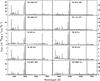 |
Fig. 4 continued. |
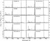 |
Fig. 4 continued. |
IRAF is distributed by the National Optical Astronomy Observatory, which is operated by the Association of Universities for Research in Astronomy, Inc., under cooperative agreement with the National Science Foundation.
Acknowledgments
N.G.G. and Y.I.I., K.J.F. are grateful to the staff of the Max-Planck-Institute für Radioastronomie (Bonn) for their hospitality and acknowledge support through DFG grant No. FR 325/59-1. Y.I.I. thanks the Observatoire de Paris for hospitality and financial support. P.P. has been supported by a Ciencia 2008 contract, funded by FCT/MCTES (Portugal) and POPH/FSE (EC), and by the Wenner-Gren Foundation.
References
- Asplund, M., Grevesse, N., Sauval, A. J., & Scott, P. 2009, ARA&A, 47, 481 [NASA ADS] [CrossRef] [Google Scholar]
- Bohlin, R. C. 1996, AJ, 111, 1743 [NASA ADS] [CrossRef] [Google Scholar]
- Campbell, A., Terlevich, R., & Melnick, J. 1986, MNRAS, 223, 811 [NASA ADS] [CrossRef] [Google Scholar]
- Colina, L., & Bohlin, R. C. 1994, AJ, 108, 1931 [NASA ADS] [CrossRef] [Google Scholar]
- Davey, A. R., Storey, P. J., & Kisielius, R. 2000, A&AS, 142, 85 [NASA ADS] [CrossRef] [EDP Sciences] [Google Scholar]
- Esteban, C., Bresolin, F., Peimbert, M., et al. 2009, ApJ, 700, 654 [NASA ADS] [CrossRef] [Google Scholar]
- García-Rojas, J., & Esteban, C. 2007, ApJ, 670, 457 [NASA ADS] [CrossRef] [Google Scholar]
- Garnett, D. R. 1992, AJ, 103, 1330 [NASA ADS] [CrossRef] [Google Scholar]
- Garnett, D. R., Skillman, E. D., Dufour, R. J., et al. 1995, ApJ, 443, 64 [NASA ADS] [CrossRef] [Google Scholar]
- Garnett, D. R., Shields, G. A., Peimbert, M., et al. 1999, ApJ, 513, 168 [NASA ADS] [CrossRef] [Google Scholar]
- Guseva, N. G., Izotov, Y. I., & Thuan, T. X. 2006, ApJ, 644, 890 [NASA ADS] [CrossRef] [Google Scholar]
- Guseva, N. G., Izotov, Y. I., Papaderos, P., & Fricke, K. J. 2007, A&A, 464, 885 [NASA ADS] [CrossRef] [EDP Sciences] [Google Scholar]
- Guseva, N. G., Papaderos, P., Meyer, H. T., Izotov, Y. I., & Fricke, K. J. 2009, A&A, 505, 63 [NASA ADS] [CrossRef] [EDP Sciences] [Google Scholar]
- Izotov, Y. I., & Thuan, T. X. 1999, ApJ, 511, 639 [NASA ADS] [CrossRef] [Google Scholar]
- Izotov, Y. I., & Thuan, T. X. 2004, ApJ, 602, 200 [CrossRef] [Google Scholar]
- Izotov, Y. I., Stasińska, G., Guseva, N. G., & Thuan, T. X. 2004, A&A, 415, 87 [NASA ADS] [CrossRef] [EDP Sciences] [Google Scholar]
- Izotov, Y. I., Stasińska, G., Meynet, G., Guseva, N. G., & Thuan, T. X. 2006, A&A, 448, 955 [NASA ADS] [CrossRef] [EDP Sciences] [Google Scholar]
- Izotov, Y. I., Guseva, N. G., Fricke, K. J., & Papaderos, P. 2009, A&A, 503, 61 [NASA ADS] [CrossRef] [EDP Sciences] [Google Scholar]
- Izotov, Y. I., Guseva, N. G., & Thuan, T. X. 2011, ApJ, 728, 161 [NASA ADS] [CrossRef] [Google Scholar]
- Kehrig, C., Vílchez, J. M., Telles, E., Cuisinier, F., & Pérez-Montero, E. 2006, A&A, 457, 477 [NASA ADS] [CrossRef] [EDP Sciences] [Google Scholar]
- Kobayashi, C., Umeda, H., Nomoto, K., Tominaga, N., & Ohkubo, T. 2006, ApJ, 653, 1145 [NASA ADS] [CrossRef] [Google Scholar]
- Kobulnicky, H. A., & Skillman, E. D. 1998, ApJ, 497, 601 [NASA ADS] [CrossRef] [Google Scholar]
- Kunth, D., & Sargent, W. L. W. 1983, ApJ, 273, 81 [NASA ADS] [CrossRef] [Google Scholar]
- Lodders, K. 2003, ApJ, 591, 1220 [NASA ADS] [CrossRef] [Google Scholar]
- Masegosa, J., Moles, M., & Campos-Aguilar, A. 1994, ApJ, 420, 576 [NASA ADS] [CrossRef] [Google Scholar]
- Melbourne, J., & Salzer, J. J. 2002, AJ, 123, 2302 [NASA ADS] [CrossRef] [Google Scholar]
- Meynet, G., & Maeder, A. 2002, A&A, 390, 561 [NASA ADS] [CrossRef] [EDP Sciences] [Google Scholar]
- Oke, J. B. 1990, AJ, 99, 1621 [NASA ADS] [CrossRef] [Google Scholar]
- Papaderos, P., Guseva, N. G., Izotov, Y. I., et al. 2006, A&A, 457, 45 [NASA ADS] [CrossRef] [EDP Sciences] [Google Scholar]
- Papaderos, P., Guseva, N. G., Izotov, Y. I., & Fricke, K. J. 2008, A&A, 491, 113 [NASA ADS] [CrossRef] [EDP Sciences] [Google Scholar]
- Peimbert, A., Peimbert, M., & Ruiz, M. T. 2005, ApJ, 634, 1056 [NASA ADS] [CrossRef] [Google Scholar]
- Pérez-Montero, E., & Díaz, A. I. 2003, MNRAS, 346, 105 [NASA ADS] [CrossRef] [Google Scholar]
- Pérez-Montero, E., & Díaz, A. I. 2005, MNRAS, 361, 1063 [NASA ADS] [CrossRef] [Google Scholar]
- Press, W. H., Teukolsky, S. A., Vetterling, W. T., & Flannery, B. P. 1992, Numerical recipes in FORTRAN, The art of scientific computing, 2nd edn. (Cambridge: University Press) [Google Scholar]
- Smith, L. J., Norris, R. P. F., & Crowther, P. A. 2002, MNRAS, 337, 1309 [NASA ADS] [CrossRef] [Google Scholar]
- Stasińska, G. 2005, A&A, 434, 507 [NASA ADS] [CrossRef] [EDP Sciences] [Google Scholar]
- Storey, P. J. 1994, A&A, 282, 999 [NASA ADS] [Google Scholar]
- Terlevich, R., Melnick, J., Masegosa, J., Moles, M., & Copetti, M. V. F. 1991, A&AS, 91, 285 [NASA ADS] [Google Scholar]
- Thuan, T. X., & Izotov, Y. I. 2005, ApJS, 161, 240 [NASA ADS] [CrossRef] [Google Scholar]
- Thuan, T. X., Izotov, Y. I., & Lipovetsky, V. A. 1995, ApJ, 445, 108 [NASA ADS] [CrossRef] [Google Scholar]
- van Zee, L., & Haynes, M. P. 2006, ApJ, 636, 214 [NASA ADS] [CrossRef] [Google Scholar]
All Tables
Electron temperatures and electron number densities derived from emission line flux ratios.
All Figures
|
Fig. 5 Comparison of electron temperatures te(O iii) (te = 10-4 Te) obtained from [O iii]λ4363/(λ4959 + λ5007) and te(S iii) obtained from [S iii]λ6312/λ9069 emission-line ratios. VLT/UVES data are shown by stars, except for three objects with uncertain values, which are shown as open circles (see Sect. 3.1). Twenty-seven data points from SDSS DR3 (see text) are shown by red dots. Open blue diamonds, blue asterisks, and purple triangles correspond to data from Kehrig et al. (2006), Pérez-Montero & Diaz (2003) and García-Rojas & Esteban (2007), respectively. The dashed blue line in the upper panel connects locations of equal temperature. The thick blue lines (also in the upper panel) are the predicted te(S iii) – te(O iii) relations for H ii region models from Izotov et al. (2006). The dotted and thin solid black lines are the curves from Garnett (1992) and Pérez-Montero & Diaz (2005), respectively. Regression lines (solid lines) and 1σ alternatives (dashed lines) for all our data plus data from García-Rojas & Esteban (2007) are shown by purple lines. In the lower panel the error bars are shown for the VLT, SDSS, and García-Rojas & Esteban (2007) data. Additionally, regression lines for VLT+SDSS-only data are shown by black lines. (A color version of this figure is available in the online journal.) |
| In the text | |
|
Fig. 6 Comparison of electron temperatures te(O iii) (te = 10-4 Te) obtained from [O iii]λ4363/(λ4959 + λ5007) and te(N ii) obtained from [N ii]λ5755/λ6583 emission-line ratios. VLT/UVES and FORS data are shown by stars, except for two objects, which are shown as open circles (see text). Green asterisks and open purple triangles provide the data from Esteban et al. (2009) and García-Rojas & Esteban (2007), respectively. The thick blue lines show the predicted te(O ii) – te(O iii) relation for H ii region models from Izotov et al. (2006). Regression lines (solid lines) and 1σ alternatives (dashed lines) for all data are shown by purple lines. The lower panel shows the error bars. Additionally, regression lines for our VLT-only data are shown by black lines. (A color version of this figure is available in the online journal.) |
| In the text | |
|
Fig. 7 Comparison of electron temperatures te(O iii) (te = 10-4 Te) derived from [O iii]λ4363/(λ4959 + λ5007) and te(O ii) obtained from [O ii]λ3727/(λ7320 + λ7330) emission-line ratios. VLT/UVES and FORS data are shown by red stars and blue filled circles, respectively. The thick blue lines represent the te(O ii) – te(O iii) relations from Izotov et al. (2006). (A color version of this figure is available in the online journal.) |
| In the text | |
|
Fig. 8 Comparison of electron temperatures te(O iii) (te = 10-4 Te) obtained from [O iii]λ4363/(λ4959 + λ5007) and te(S ii) obtained from [S ii]λ4068/(λ6717 + λ6730) emission-line ratios. Symbols are the same as in Fig. 7. Regression lines for all data are represented by purple lines. Regression lines for the UVES-only data are shown by black lines. (A color version of this figure is available in the online journal.) |
| In the text | |
|
Fig. 9 Ne(O ii) versus Ne(S ii). Black stars: VLT-UVES; filled blue circles: FORS observations (medium resolution). Purple triangles: data from García-Rojas & Esteban (2007), green asterisks: data from Esteban et al. (2009). The dashed blue line connects points of equal densities. The lower panel shows the error bars and regression lines and their 1σ alternatives for all data (purple lines) and for the VLT-only data (black lines). (A color version of this figure is available in the online journal.) |
| In the text | |
|
Fig. 10 Ne(Cl iii) versus Ne(S ii). UVES, FORS and SDSS DR3 data are represented by black stars, filled blue circles, and red dots, respectively. Purple triangles: data from García-Rojas & Esteban (2007), green asterisks: data from Esteban et al. (2009). The dashed blue line connects points of equal densities. The lower panel shows the error bars. (A color version of this figure is available in the online journal.) |
| In the text | |
|
Fig. 11 Ne(Ar iv) versus Ne(S ii). FORS data are represented by filled blue circles. Purple triangles: data from García-Rojas & Esteban (2007), green asterisks: data from Esteban et al. (2009). The dashed blue line connects points of equal densities. The lower panel shows the error bars. (A color version of this figure is available in the online journal.) |
| In the text | |
|
Fig. 12 log N/O a), log Ne/O b), log S/O c), log Cl/O d), log Ar/O e) and log Fe/O f) vs. oxygen abundance 12 + log O/H for our sample of 121 spectra (large stars). Several knots in H ii regions NGC 346 and NGC 456 in the SMC are shown by green and purple large asterisks, respectively. Additionally we show the galaxies from the HeBCD sample of Izotov et al. (2004) and Izotov & Thuan (2004) for the primordial He abundance determination (small filled blue circles) and the sample of ~300 emission-line galaxies from the SDSS DR3 (Izotov et al. 2006) (red dots). The solar abundance ratios by Lodders (2003) and by Asplund et al. (2009) are indicated by the purple and black large open circles and the associated error bars. The straight black lines are linear regressions for the HeBCD sample by Izotov et al. (2006) and the purple ones are for all (except the SDSS data). The right panel shows the error bars. (A color version of this figure is available in the online journal.) |
| In the text | |
|
Fig. 13 Comparison of the abundance discrepancy factor ADF = log O++(RL)/O++(CEL) with observed F(Hβ). Data from UVES and FORS medium resolution observations are shown by red stars and filled blue circles. Green asterisks are the data from Esteban et al. (2009). (A color version of this figure is available in the online journal.) |
| In the text | |
|
Fig. 14 Dependence of the ion abundance ratio log C++(RL)/O++(RL) on 12 + log O/H(CEL). Our data are marked by the same symbols as in Fig. 13. Data from Garnett et al. (1995) and García-Rojas & Esteban (2007) are shown by filled and open purple triangles, respectively. Green asterisks are the data from Esteban et al. (2009). Data from Garnett et al. (1999) and Kobulnicky & Skillman (1998) are shown by light blue squares and black circles, respectively. (A color version of this figure is available in the online journal.) |
| In the text | |
|
Fig. 1 Optical images of the galaxies. The straight lines indicate the location of the slit during observations (see Table 1). |
| In the text | |
|
Fig. 1 continued. |
| In the text | |
|
Fig. 1 continued. |
| In the text | |
|
Fig. 1 continued. |
| In the text | |
|
Fig. 1 continued. |
| In the text | |
|
Fig. 2 Flux-calibrated and redshift-corrected UVES spectra of galaxies. |
| In the text | |
|
Fig. 2 continued. |
| In the text | |
|
Fig. 2 continued. |
| In the text | |
|
Fig. 2 continued. |
| In the text | |
|
Fig. 2 continued. |
| In the text | |
|
Fig. 2 continued. |
| In the text | |
|
Fig. 3 Flux-calibrated and redshift-corrected FORS low-resolution spectra of galaxies. |
| In the text | |
|
Fig. 3 continued. |
| In the text | |
|
Fig. 3 continued. |
| In the text | |
|
Fig. 4 Flux-calibrated and redshift-corrected FORS medium-resolution spectra of galaxies. |
| In the text | |
|
Fig. 4 continued. |
| In the text | |
|
Fig. 4 continued. |
| In the text | |
Current usage metrics show cumulative count of Article Views (full-text article views including HTML views, PDF and ePub downloads, according to the available data) and Abstracts Views on Vision4Press platform.
Data correspond to usage on the plateform after 2015. The current usage metrics is available 48-96 hours after online publication and is updated daily on week days.
Initial download of the metrics may take a while.