| Issue |
A&A
Volume 549, January 2013
|
|
|---|---|---|
| Article Number | A65 | |
| Number of page(s) | 15 | |
| Section | Interstellar and circumstellar matter | |
| DOI | https://doi.org/10.1051/0004-6361/201219263 | |
| Published online | 19 December 2012 | |
High-resolution spectra of the planetary nebula NGC 6803⋆
Department of Earth Science (Astronomy), Chungbuk National University, Cheongju, Chungbuk 561-756, South Korea
e-mail: This email address is being protected from spambots. You need JavaScript enabled to view it.
Received: 22 March 2012
Accepted: 26 October 2012
Abstract
We present the high-dispersion spectra of the elliptical ring shaped planetary nebula NGC 6803, secured with the Hamilton Echelle Spectrograph attached to the 3-m Shane telescope of Lick Observatory. Numerous lines from neutral to quadruply ionized ions are presented in the wavelength region from 3650 to 9900 Å. We also use the low dispersion UV spectral data obtained with the 60-cm interstellar ultraviolet explorer. In spite of its simplistic symmetrical bilateral shape, the diagnostics imply that the physical condition of the nebular shell is very complex with a huge density range of 1300−80 000 cm-3. A comparison of the 1995 and 2001 [Ar iv] data suggests that the density increase occurred near the inner shell boundary. In spite of a huge ionization potential range, the average electron temperature indicated by primary diagnostic lines is relatively low, i.e., Te ≤ 9500 K, except for [Cl iv], from which we derive a temperature that is around 11 500 K. We derived the chemical abundances of He, C, N, O, Ne, S, Ar, Cl, and K, based on the physical condition suggested by diagnostics and photo-ionization analysis. The chemical abundances of NGC 6803 are mostly enhanced when compared with the average Galactic planetary nebula. The effective temperature of its central star appears to be about 90 000 K and its luminosity about 2400 L⊙, assuming a distance of 3000 pc. The evolutionary track implies that NGC 6803 might have been evolved from a companion star of about 1.0 M⊙ in a binary system, or from a single progenitor of about 1.5 M⊙, born in a metal-rich zone near the Galactic plane.
Key words: planetary nebulae: individual: NGC 6803 / ISM: abundances / Stars: AGB and post-AGB / HII regions / planetary nebulae: general
Table 2 is available in electronic form at http://www.aanda.org
© ESO, 2012
1. Introduction
An intermediate star of 1−8 M⊙ evolves on an asymptotic giant branch (AGB), which ejects a large fraction of material into the interstellar medium (ISM). The ejected gas is brightened by the hot stellar core at the end of the AGB and begins a new evolutionary phase as a planetary nebula (PN). The nebulous gas that surrounds the central star of the planetary nebula (CSPN) is brightest in the optical wavelength range. Numerous lines are emitted from the PN in a broad spectrum of wavelengths ranging from UV to IR, where an especially large portion observed is in the visual wavelength range. The high-dispersion spectroscopy is useful in discerning the closely located lines, such as [N i] 5198 & 5200, [Ne iii] 3967 & 3970, and [O ii] 3726 & 3729 (all line wavelengths are in Å unit), whose intensity ratios allow us to derive the physical condition of the nebular shell. The spectroscopic studies based on the high-dispersion spectroscopic data in the optical wavelength regions can reveal information on rare elements, such as Cl, K, Ar, and F, which supply further clues to their origin or build-up history, which would have occurred along the evolutionary track of low-to-intermediate massive stars (see, e.g., Otsuka et al. 2008).
NGC 6803 is a relatively small, bright PN that shows a disk with a bright, elliptical, shaped rim, 6 . It is known as a moderate excitation object with He ii 4686 and [O ii] 3727 that are weak (Lee et al. 1974; Aller 1951). Feibelman (1994) detected the P Cygni signature in C iv from the IUE spectral data.
Understanding the physical conditions of the PN gas and the CSPN is very important. Peimbert & Torres-Peimbert (1987) studied the density and temperature dependence of the He i I(10830)/(5876), along with I(7065)/(5876) ratios observed in NGC 6803. Zhang et al. (2004) have derived the physical conditions and chemical abundances of NGC 6803 based on the medium-resolution data, at 0.95−4 Å. It would be more useful if one can find the physical state of this object using high-resolution data, e.g., 0.05−0.154 Å available with the Hamilton Echelle Spectrograph (HES) attached to the 3.0-m Shane telescope at the Lick Observatory. Most recently, the spectroscopic line profile analysis has been carried out using HES data by Choi et al. (2008). However, the objective of their study was to study the expansion velocity of the shell based on the line profiles of some strong lines.
In this study, we present the full list of optical lines secured with the 3-m HES. We also measure the UV emission lines available through the IUE archives. Using these data, we obtain the physical condition of NGC 6803 and derive chemical abundances. We also construct a photo-ionization (P-I) model and derive properties of the CSPN.
Section 2 presents the line fluxes from the IUE and HES observations. In Sect. 3, we discuss the physical conditions derived from the diagnostic lines. In Sect. 4, we give the derived chemical abundances with the help of a theoretical model. Section 5 gives a summary. Table 1 lists some basic data for NGC 6803.
Some basic data for NGC 6803, PNG 046.4−04°1.
2. Spectroscopic data
The HES spectroscopic observations were carried out with the 3-m telescope at the Lick Observatory on 1995 August 18 (UT) and 2001 August 29 (UT). The detailed description of the HES observations is given in Choi et al. (2008), who present the spectral line profiles using the 1995 spectral data for their line profiles. In this study, we used two types of observation data. The exposures were 120 and 3 min in 1995, and 60 and 5 min in 2001. The description of the two short exposures given in Choi et al. (2008) was wrong (Choi, priv. comm.), which reported as two and three minutes in 1995 and 2001, respectively. The seeing was about  during the observations. We placed a slit entrance of 640 μm (~1.′′2) × 4.′′0 at the center of the planetary nebula. The chosen slit width of 640 μm corresponds to two pixels on a 2048 × 2048 CCD or a spatial dimension of 1.′′2 in the sky. The two pixels on a CCD in our HES system correspond to 0.05 Å at 3600 Å and 0.15 Å at 8850 Å, respectively.
There was no fixed position angle, since no image rotator was used in the observing run; when the observation started, the slit length direction was set in a vertical axis on a randomly directed image and the nebular image was rotated on the slit entrance during the exposures. Although there appears to be no prominent small-scale structure(s) from ground-based telescopic images, there could be some small sub-arc-second structures that might cause the intensity difference between different observing runs. Any further discussion remains speculative until high spatial resolution images are available, e.g., with Hubble space telescopic observations.
The data reduction was carried out by the IRAF. The detailed data reduction procedures are described in Hyung (1994). Table 2 lists the optical region HES spectra, combined from four exposures of 1995 and 2001 observations: (1) Lines of the strong Hα and [O iii] 4959, 5007 were often saturated in long exposures, so we need to use data from short exposures; (2) We also listed some questionable lines (marked as “line?”), leaving their identification to a future study. The first column gives the measured wavelength corrected for the nebular radial velocity with respect to the observer, 10.23 ± 0.75 km s-1. This value was obtained by comparing the observed wavelengths of all the relatively strong lines (F(HES) > 1.0 relative to F(Hβ) = 100.0) with the laboratory wavelengths in column 2. The radial velocity derived by Hβ lines is 15.80 km s-1, which is close to the Acker et al. (1992) quoted value, Vr = 13.1 km s-1. The discordance may be caused by the different choice of data: the kinematical structure responsible for certain species of ions must be different from that of other lines. It also may be affected by different observation conditions, e.g., different area over the image, different slit entrance size, and different devices employed.
Observed emission line fluxes from low-dispersion IUE spectra.
Columns 3 and 4 of Table 2 are the ions and the multiplet number in Moore’s Multiplet Table (Moore 1972). Column 5 gives the extinction coefficient, fλ, as defined by Seaton (1979). Column 6 gives the extinction corrected HES flux line intensities, while Cols. 8 and 9 list the 1995 and 2001 HES intensities, respectively, all on the scale of I(Hβ) = 100.0. Column 7 lists root-mean-square (rms) errors estimated from all the available 1995 and 2001 HES four exposures.
Diagnostic indicated physical conditions.
The logarithmic interstellar extinction coefficient at Hβ can be derived from a comparison of the observed Balmer line ratios with the theoretical values (Hummer & Storey 1987). Lee et al. (1974) found C = 0.6 assuming electron temperature, Te = 7500 K, while Zhang et al. (2004) derive C = 0.869. Choi et al. (2008) assumed C = 0.63 for their line profile study with the 1995 data. From the current combined data set, we adopted a slightly higher value, C = 0.81 or Av = 1.71. The scatter is unavoidable considering the different slit position and size over the nebular image and seeing conditions at the time of the run. The different choice of C would not change our conclusion. The higher extinction value, C, implies that NGC 6803 is heavily affected by the interstellar extinction due to the low Galactic latitude and possibly due to the farther distance from us.
The IUE archives contain two spectral scans, SWP06256 and LWR05428 (1979 August 23, Program ID: NCBJH, PI: Harrington), taken with the large (10 × 23 arcsec2) entrance aperture. The exposures of both data were each an hour long. The measured UV line fluxes are given in Table 3. We were able to measure about a dozen lines including two strong lines of He ii 1640 and C iii] 1908, but most other lines were very weak. The employed HES entrance-slit size was smaller than the nebula. Meanwhile, the IUE oval slot entrance size was larger, so all the flux is expected to have been captured in the IUE observation. Since the IUE and HES observations employed different slot entrances and as a result the spectral data represent different areas of the nebula, one cannot find the exact the extinction coefficient for the IUE data. We applied extinction coefficient, C = 0.81, to the IUE data, derived from the HES data. Here we employed a theoretical ratio of I(He ii 1640)/I(He ii 4686) = 6.7 (for Te = 11 000 K), assuming the electron temperature indicated by the other high-excitation HES [Cl iv] line (see Fig. 1).
We were able to observe the following lines: H, He i, He ii, C ii, C iii], C iv], [N i], [N ii], N ii, N iii, [O i], O i, [O ii], O ii, [O iii], O iii, [Ne iii], [S ii], [S iii], [Ar iii], [Ar iv], [Ar v], [Cl ii]?, [Cl iii], [Cl iv], Si ii, [Fe ii], [Fe iii], [Fe vii]?, [K iv], and Mg i. The [Fe vii] and [Cl ii] lines are questionable. The high excitation He ii, [Ar v], and [Cl iv] lines are present. The weakly registered O iv] and [Ne iv] in Table 3 appear to be real. The O iii lines in both HES and IUE could be real and might be Bowen fluorescence lines. Over about 190 lines are identified. We also list unknown ~70 lines, marked as “line?”, for a future study.
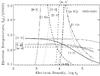 |
Fig. 1 Electron temperature and density of NGC 6803, based on the combined data. |
As noted by Lee et al. (1974), the He ii lines are weak, as well as other high-excitation lines such as [Cl iv] and [K iv]. The low-excitation lines are also very strong. The diversified excitation implies that the nebular geometry is much more complex than one can guess from its simple appearance. In the next section, we derive the physical conditions based on the diagnostic lines in Tables 2 and 3.
Separate measurement of diagnostic line intensities in each exposure.
3. Nebular physical conditions
With the atomic constant as given in Aller (1984) and Osterbrock (1989), the ratios of some diagnostically useful lines would allow us to derive the electron temperatures and densities of the gas. The recent up-to-date data can be found in Otsuka et al. (2009). Table 4 gives the nebular physical conditions, Te and log Ne, derived based on the combined line intensities, I(HES), i.e., Col. 6 of Table 2, while Fig. 1 displays a diagram that plots the locations of the physical conditions, log Ne − Te plane. The lines we have used were [N i] 5198/5200, [N ii] 5755/(6548+6583), [O ii] 3726/3729, [O ii]a (3726+3729)/(7319+7330), [O iii] (4959+5007)/4363, [S ii] 6716/6731, [S ii]a (6716+6731)/(4069+4076), [S iii] (9069+9531)/6312, [Ar iii] (7751+7136)/5192, [Ar iv] 4711/4740, [Ar iv]a (4711+4740)/7171, [Cl iii] 5518/5538, and [Cl iv] 5323/(7530+8045). Successive columns in Table 4 stand for ion, ionization potential (I.P.), related diagnostic lines, line ratio along with the rms % error obtained from the combined HES data, given in parenthesis, and derived Tes or Nes for the combined (1995+2001), 1995, and 2001 HES data.
In deriving the [O iii] electron temperature, we used the well-known (4959+5007)/4363 line ratios. However, some lines such as 4959+5007 lines are strong, so the line measurements are only available from the short exposures. Weak lines, which are missing in the short exposures, can sometimes be available from the long exposures. For the strong lines, the opposite is true. Table 5 illustrates the situation for which lines are available and for which ones are missing in the long and short exposures of HES, respectively.
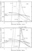 |
Fig. 2 Electron temperature and density of NGC 6803. Top: with the 1995 data. (Number 2: from a short 3 min. exposure. Unspecified diagnostic lines are from the 120 min. exposure data.) Bottom: with the 2001 data. (Numbers 3 and 4: 60 and 5 min. exposures. The unspecified diagnostics are from the 60 min. one.) |
Hyung et al. (1994a,b) estimated the diagnostic error with the HES data: e.g., △ T = ± 1500 K for ~6% errors in [Ar iii] lines, and △ log Ne = ± 0.2 dex for ~10% in [Cl iii] lines. We similarly estimated the errors for the diagnostic derivation, based on the highest rms value from the lines involving each ratio, △ T < 350 K, except for [Cl iv] and △ log Ne < 0.11 except for [O ii]. Part of the scatter is due to observational or measurement error. The scatter could also be caused by the error in atomic constants or by incomplete correction of interstellar and atmospheric extinction, especially when the wavelength separation involving the diagnostic line ratio is large as apparent in [S iii] (9069+9531)/6312 and [O ii] (3726+3729)/(7319+7330).
The diagram indicates that the electron temperatures are about Te ~ 8500 − 9500 K for most ions, assuming log Ne = 4.0. From their 1995 HES data analysis (with a slightly different C parameter), Choi et al. (2008) find a similar Te([O iii]) = 9700 K. Lee et al. (1974) derived electron temperatures and densities using their photographic and photoelectric data, Te([O iii]) = 9500 K and Te ~ 7500 K from the Balmer jump. Zhang et al. (2004) find a similar electron temperature, Te ~ 9730 K from the [O iii] (88 μm + 52 μm)/4959 lines. They also derive another electron temperature, Te ~ 8500 K and log Ne = 3.6 from the Balmer jump. There is only one measurement of [Cl iv] from the 1995 2 h exposure, which indicates a higher Te of around 11 000 K. The [N ii] electron temperature would also be higher if we assume a lower density for the low excitation lines. The high temperature indicated by [Cl iv] might be in error, since the [Cl iv] 5323 line is weak (low S/N).
The electron densities are more complex, i.e., Ne ~ 1300−80 000 cm-3. We may be able to distinguish them in three Ne domains; (1) Ne ~ 13 000 cm-3 for most ions; (2) Ne ~ 1300−2800 cm-3 for low-excitation lines, such as [N i] and [O ii]; and (3) Ne ~ 55 000−80 000 cm-3 for some auroral-to-nebular transition lines, [Ar iv]a and [O ii]a. The electron densities derived by Choi et al. (2008) were 2000−9000 cm-3, assuming 9700 K, i.e., high density for the high-excitation lines and low density for the low-excitation lines. Choi et al. (2008) interpret the density scatter as a density contrast in a prolate shell. See their Fig. 2, where the model geometry of a prolate shell is found, in which the density of the equatorial shell is much higher than that of the polar conic zone. The discordance of densities derived by the same ionic stage could be due to the atomic constants although the degree of uncertainties would be different depending on different ions (see Wang et al. 2004 for more details). With caution, the present diagnostics indicate the possibility of much higher density substructures.
Derivation of the diagnostic temperatures or densities based on the averaged intensities of the two different epochs could be wrong in the case of flux changes. We present the electron temperatures and densities, Cols. 7 − 8 in Table 4 for two epochs separately. Figure 2 shows the diagnostics of 1995 and 2001 separately, which was observed with the same spectrograph.
The electron temperatures show a decrease. The change appears to be obvious in [Ar iii] and [O iii], but the indication coming from [S iii] is uncertain. No notable variations are found in density diagnostics, except for [Ar iv] between the 1995 and 2001 epochs. To verify whether the change in the [Ar iv] diagnostic is real, one must evaluate the errors in this and other diagnostics.
Estimating scatter in the derived diagnostic temperatures or densities using the rms % of several different epoch line intensities might not be useful, especially when the actual change occurs in the line fluxes. For the 1995 and 2001 data, one can similarly estimate the scatters, using the rms % errors presented in Table 2.
Diagnostic line ratios and errors for all exposures.
Table 6 presents the separate line intensity ratios for four exposures, along with rms % errors for each epoch, i.e., 1995 and 2001 HES data, respectively. The rms % error for each line ratio was in fact adopted from the maximum errors of the lines involved. Since the rms % errors are not available for [Cl iv ] and [N i ] , we quote from [Cl iii ] . The rms % errors of each epoch are much smaller than those of the total I(HES) (see rms % errors in parenthesis, Col. 4 of Table 4). We did not present the resulting diagnostic scatters for two epochs in Table 4, since they would be smaller than those of Col. 5 in Table 4.
Derivation of ionic concentrations.
Both 1995 and 2001 diagnostics in Fig. 2 generally agree with the combined result in Fig. 1 within an observation error. There appears to be an abnormally large difference in Ne([Ar iv]), △ log Ne ~ 0.21 dex, between two periods. Was there any shock activity in the high-density, inner shell boundary that caused a change in physical conditions? Although we could not extract temperature change in the high-excitation lines, there appears to be evidence of sudden density change, Ne = 8900 (103.95) → 14 400 (104.16) cm-3 between two periods. The [Ar iv] density variation found in the HES data that were obtained under similar or extremely good weather conditions appears to be an actual feature.
The density variation might occur perhaps due to some radical event, such as an interacting wind in limited zone near the inner boundary of the main shell where the [Ar iv] or other high-excitation lines were emitted. From the available IUE UV spectra, NGC 6803 was known to have a central star with weak emission lines. Feibelman (1994) suspected that NGC 6803 may have C iv P Cyg, while Marcolino et al. (2007) report it as absent. There is no evidence of any systematic change in electron densities and temperatures in other lines, though.
The discordance found in the [O ii] diagnostics was seen in other PNe: the auroral-to-nebular transition, [O ii] (7319+7330)/(3726+3729), always indicates higher density than the nebular line ratio does. Some Galactic PNe are known to be high-density objects, e.g., IC 4997 (Hyung et al. 1994b) and M 2-24 (Zhang et al. 2004). NGC 6803 would not be classified as such a high-density PN. A somewhat high-density value is also to be found from the [N ii] lines: Ne ~ 21 000 cm-3, assuming Te ~ 9000 K for the [N ii] zone. However, in a relatively low-density object like NGC 7009 (the high-dispersion long-slit spectroscopic data analysis by Hyung & Lee, in prep.), the high-density blobs or substructures appear to be present in the main shell (see also the BoBn 1 investigation by Otsuka et al. 2010). The discussion of the density fluctuation or a possible presence of high-density substructures in this object is beyond the scope of our study, so we will leave this matter to future study.
In NGC 6803, we detected the high-excitation lines such as He ii and O iv]. When compared with other high-excitation Galactic PNe that emit the He ii lines, the overall gas temperatures suggested by the diagnostics appear to be low. We need to check the electron temperatures derived by the diagnostics with the predicted values by a P-I model, and we further investigate the cause of the relatively low temperatures indicated by the [O iii] and [Ar iii] lines of the nebula.
Using the electron temperatures derived from the diagnostic lines, one can derive ionic concentrations for available ions. In deriving the fractional ionic concentration, we assumed the same electron density, Ne ~ 10 000 cm-3, for all ions, and adopted the position where the most ions crossed. The electron temperatures were adopted differently, using the diagnostic information of [Ar iii], [S iii], [O iii], and [Cl iv] ions and considering the level of the ionization potential (I.P.) of involving ions. Table 7 lists fractional ionic abundances for He+, He2+, C2+, C3+, N0, N+, N2+, O0, O+, O2+, O3+, Ne2+, Ne3+, S+, S2+, K3+, Cl2+, Cl3+, Ar2+, Ar3+, and Ar4+, mostly based on collisionally excited lines, except for He. Successive columns give ions, lines used, line intensities, electron temperatures assumed for the ions, fractional ionic concentration relative to hydrogen, and mean values. The ionic concentration of some elements, e.g., C, is only available from the UV wavelength region. The C value was from the international ultraviolet explorer (IUE) data, i.e., intercombination C lines in the UV wavelength region, e.g., C iv] 1549,51 and C iii] 1907,09 in Table 7. We derived the ionic abundances for these UV lines, assuming that the intercombination UV lines are collisionally excited.
As mentioned, NGC 6803 shows strong line intensities even for the neutral stages of O and N. Although the fractional concentration was available for oxygen, O0 or N0 value must be ignored because these ions are likely to be patches that could not represent the ionized zone. There is a large discordance in O+ or Ar3+, because some lines in these ions are strongly dependent on the density. As noted earlier, the densities found by the nebular line ratio and by the auroral-to-nebular transition line ratio were different.
For some ions such as O, most of the ionic stages were available in the presented optical HES and UV IUE wavelength range data. In such a case, the elemental abundance would be the sum of all ionic concentrations. However, for most elements, the UV data in Table 2 and the ground-based telescopic data in Table 3 did not cover all ionic stages, so one must find the ionization correction factors (ICFs) for the unobservable ionic stages to derive the abundance for each element. The ICF for the unobservable stages is usually found by using either (1) the semi-empirical method referring to the availability of other ions of similar I.P. or (2) the photoionization (P-I) modeling method utilizing its prediction.
We employ the latter method, i.e., constructing an appropriate P-I model nebula with NEBULA (Hyung 1994) and CLOUDY (Ferland 1997). In general, the chemical abundance determined by using collisional lines differs largely from that determined by using recombination lines. The standard P-I model, which assumes the permitted lines to be recombination lines, cannot fit the permitted lines in case the permitted lines are emitted through another mechanism such as fluorescence, nor can predict the shock excited lines.
We evaluate the degree of discordance for the C ii 4267 by comparing the observed intensity with the prediction in the next section.
Ionic concentration in NGC 6803.
4. Theoretical model and chemical abundances
To investigate the spectra of various elements in a self-consistent way, one needs to analyze all spectra simultaneously in a coherent environment or in a sound model. We use a P-I model with NEBULA (Hyung 1994). We also refer to the prediction by CLOUDY (Ferland 1997). Lee & Hyung (2008) have recently compared the prediction for a relatively simple structure PN, NGC 7026, using two codes, and basically found no difference between them.
Inputs for NGC 6803 P-I model.
To start a nebula model calculation with a P-I code, one must know the approximate value of chemical abundances for the gas shell and the stellar energy distribution (SED) curve for the ionizing UV photons. For the SED or the photoionizing UV continuum photons from the CSPN, “Tlusty” by Hubeny (1988) was used. We assumed the central star has the same chemical abundances as the nebular gas. The distance to the PN must also be adopted to fit the size and the absolute F(Hβ) flux. Acker (1992) gave the distance to NGC 6803 in the range 1 − 3.0 kpc. We adopted 3000 pc, close to the maximum. The chemical abundances must be given as an input. We were guided by the ionic abundances given in Table 8, and we refined them further until the P-I model calculation fit both the electron temperature(s) and the observed line intensities well.
The P-I code also requires a geometry and density distribution in the shell. The model cannot employ a realistic complex geometry or the different densities seen in the diagnostics. As a standard procedure, we start a model with a stellar radius and inner shell radius and adjust the inner and the outer boundaries to fit the observed nebular size. Once these are given, the P-I code will solve the energy balance and statistical equilibrium equations at each radius and give predictions, e.g., line fluxes, the ionization fraction for each element, and physical conditions. If the prediction does not fit the observed values, one needs to adjust the effective temperature of the CSPN, with which one must produce another SED by using “Tlusty”. The iteration goes on until the P-I model nebula gives a satisfactory prediction for the observed line intensities.
Comparison of observed and predicted intensities in NGC 6803 (I(Hβ) = 100).
The diagnostics, as shown in Figs. 1 and 2, implied a higher density, especially for the high-excitation lines. As discussed in Sect. 3, the nebular shell might consist of three different density zones. It would therefore be desirable to construct a model geometry with a density contrast between the polar and the equatorial zones (see IC 2165, Hyung 1994) or a stratified shell with a high-density compact inner shell with the outer low-density shell (see IC 4997, Hyung et al. 1994b). For NGC 6803, we do not employ such a refinement, since it does not improve the prediction except for some lines, such as [O ii]7321/2, 7332/3. Instead, we assumed a homogeneous shell with a density value, NH = 8800 cm-3 (or Ne ~ 10 000 cm-3), close to the intermediate value in Figs. 1 and 2. The single density value may cause a problem for low or high density lines, as mentioned in Sect. 3 (see Figs. 1 and 2 and Table 4). However, we believe the simplistic density distribution would not misguide our effort on chemical abundances or the CSPN parameters.
Table 9 lists the input data for the model nebula and the CSPN and the chemical abundances adopted in our final P-I model. We also list the predicted fractional ionization factor, Xn+s for all available elements and the ionization correction factors, ICFs, for the unobserved ionic stages (see Table 9). The chemical abundances appear to be enhanced (discussion will follow). As noted before, the electron temperatures of NGC 6803 indicated by the diagnostics were relatively low, in spite of the appearance of high-excitation lines, 8000, 9300, and 9500 K by [Ar iii], [S iii], and [O iii]. The Te([Ar iii]) is even lower than the Te([N ii]). We checked the O zones, where the predicted electron temperatures were 9800, 9000, 10 300, and 10 600 K for [O ii], [O iii], [O iv], and [O v], respectively. The relatively lower temperatures appear to be caused by relatively large amount of cooling elements, i.e., C/H, N/H, O/H, etc.
The final model indicated that the effective temperature of the CSPN is 90 000 K. The inner and outer shell radii are 0.015 and 0.033 pc, so the angular size of the outer radius would be ~2 at a distance of 3000 pc. The outer boundary matches the approximate size of the shell in the equatorial zone direction, which is presumably a higher density zone than the polar zone. The outer boundary of the shell is material-bounded (i.e., truncated within the Strömgren sphere radius) to fit the line intensities well. If we adopt a lower density in the shell (and with a little larger inner radius), we can similarly fit the outer boundary of the shell in the polar cap direction (~3′′).
The intrinsic absolute Hβ flux, given by the model, is F(Hβ) = 3.5(−11) (here, 3.5(−11) means, 3.5 × 10⁻¹¹ erg cm-2 Å-1 s-1). Then this value corresponds to F(Hβ) = 5.4(−12) in observation by applying the interstellar extinction, C = 0.81, which is slightly lower than the observed value of 6.6(−12), given in Table 1. One can fit the absolute Hβ flux by increasing the radii of the CSPN and nebular shell, e.g., by 1.1 times and L(⋆) ~ 2400 → 2900 L⊙. A slight increase in the CSPN radius and shell boundaries adopted in the model would not change the predicted value of the angular nebular size.
The shell itself was assumed to be homogeneous, and no filling factor was introduced. One can increase the outer boundary with the filling factor, whenever the predicted PN outer boundary is smaller.
In the study of other ring type PN Hubble 12, Hyung & Aller (1996) solved this dilemma by introducing a high-density compact shell around the CSPN, which is detached in the outer main shell. NGC 6803 could be such an object. The possible presence of a recently ejected high-density substructure in this object, however, can only be verified through a large ground telescope, such as the 8-m class Subaru, the Very Large Telescope, or the Hubble Space Telescope. As mentioned earlier, the distance adopted in the model is an upper limit (see Table 1). Putting the nebula at a farther distance would make the predicted Hβ flux CSPN brightness lower. The current adopted distance appears to be the best choice.
Comparison of abundances.
In Table 10, we list the predictions. The observed and predicted line intensities are all given on the scale of I(Hβ) = 100. The predictions were generally successful for most lines except for auroral transition lines such as [O ii] and [S ii], and the agreements for He i and He ii are generally fine. In predicting He lines, we corrected for collisionally excited contributions. For the cases of N and O, there are strong forbidden lines in the optical wavelength region, whereas there is no strong forbidden line for C in the optical wavelength region. We must therefore rely on the UV lines for C. The predictions for UV C iii] 1907/09, C iv] 1549/51, and optical C ii 4267 are fine. Considering that the observed line intensities of permitted lines are often stronger than the predicted values by 3–20 times, the prediction for C ii 4267 is surprising.
It has been a long-standing problem that contemporary available P-I codes cannot predict both forbidden and recombination (permitted) line intensities simultaneously. Our P-I modeling was carried out to fit the forbidden lines. We also checked the predicted values for the relatively stronger permitted lines of N iii (assuming these are recombination lines), but discrepancies are large. For example, Iobs & Ipred = 1.28 & 0.20 for N iii 4640.6, and 1.20 & 0.06 for N iii 4641.8. The predicted values for the other recombination lines, N iii 4097 and N iii 4103, are less than 0.01 (but Iobss = 1.54 & 0.74, respectively). A comparison of predictions for other weakly observed O ii and O iii lines is not applicable (Ipred < 0.01), unless we increase the input values for these elements to fit the line intensities. We did not try such a refinement. The discrepancy for the prediction of N3+ permitted lines (due to the presently adopted abundance suitable for the forbidden N lines) is greater by a factor of six. Wesson et al. (2005) find a smaller abundance disagreement between the recombination line method and the forbidden line method: 4.5, 2.8, and 3.1 times for C, N, and O, respectively. Our discrepancies for C ii, which only comes down to a factor of two, is quote low compared with those of other permitted lines.
These scatters or disagreements are perhaps due to observational errors involving the bad weather condition and errors caused by data reduction, e.g., atmospheric correction and the response function from the flux calibration star. The other error sources are the atomic constants employed in the code and the assumed simplistic nebular geometry. Predictions for ions of N, O, Ne, and Cl are generally successful. As mentioned earlier, the discordance for some [S iii], [O ii], and [Ar iv] lines are unavoidable with the simplistic single-density shell. The actual object may consist of complex high-density blobs within the main shell and the shell itself may have a stratified radial density variation. As mentioned, a density-contrast shell model would be desirable, but we did not try such a refinement to improve the predictions.
With the P-I model predictions, we are now able to find the semi-empirical abundances for He, C, N, O, Ne, S, Cl, Ar, and K. We derived them, all based on the model, for collisionally excited lines. In Table 11, we compared the abundances of He/H, C/H, N/H, O/H, Ne/H, S/H, Cl/H, and Ar/H. Column 2 gives the ionic abundances of observed stages, i.e., IUE and HES data (Table 6). Column 3 lists the P-I model’s ICFs in Table 9, Column 4 gives the semi-empirical ICF abundances by multiplying both Cols. 2 and 3. Column 5 lists the P-I abundances presented in Table 9. Column 6 gives the logarithmic difference, i.e., △ = log N(ICF) − log N(P-I). The abundance difference between two methods agrees within a factor of two except for C, N, and S, where △ = 1.89, − 0.69, and 1.01, respectively. We also quoted other derivations by Wesson et al. (2005) in Col. 7 for comparison. Column 8 lists the recommended abundances close to the middle of the two N(ICF) and N(P-I) values; 9 the average PN value by Kingsburgh & Barlow (1994); and 10 the solar values quoted from Hyung & Feibelman (2004).
Although the C, N, and S abundances are uncertain, NGC 6803 is an O/C > 1. The typical Galactic PN has a carbon-to-oxygen ratio (C/O) greater than unity, while NGC 6803’s C/O is less than 1 or oxygen-rich. Our recommended abundances are close to the values derived by Wesson et al. (2005) except for Ne. Most elemental abundances are higher than the average Galactic PN values except for C and Cl. The He and N are slightly enhanced object, and the Ne and S are also enhanced. M-type AGB stars are known to have an oxygen-rich atmosphere, while C-type AGB stars have a carbon-rich atmosphere. The triple-α process inside the AGB star may produce 12C. The carbon is dredged up to the surface, which changes the chemical composition of the atmosphere. If the carbon-to-oxygen ratio (C/O) is less than unity, carbon atoms will be locked into the CO around the star. The later stage or PN will thus be oxygen-rich. On the other hand, if the carbon processed in the helium-burning regions of AGB is continuously dredged up, the surface of the star changes from an oxygen-rich to a carbon-rich environment (see, e.g., Otsuka et al. 2010). NGC 6803 did not undergo such a continuous or third dredge-up. NGC 6803 must have evolved from an O-rich, M-type AGB star.
The nebular radial velocity to the Sun is ~ 10.23 (13.1) km s-1 and the Galactic longitude of NGC 6803 (l = 46 & b =
& b =  ; 2000) is close to the position of solar apex. The solar motion relative to the local standard of rest (LSR) is ~ 13.4 km s-1 toward a position of Hercules (l ~ 50°, b = + 23°). The radial velocity of NGC 6803 relative to the LSR would be ~25 km s-1, which is similar to that of other Galactic PNe (Hyung & Huh 2007) or the nearby later generation of Galactic members, such as metal-rich main sequence A stars (Carroll & Ostlie 2007; see reference therein). The radial distance of NGC 6803 from the Galactic center is ~6.3 kpc, assuming that the Sun’s distance to the Galactic center is 8.0 kpc and the distance to the PN from us is 3 kpc. As a result, NGC 6803, located closer to the the Galactic center than the Sun, must be rotated around the Galactic center at a faster velocity than the Sun, similar to what other nearby Galactic PNe do. The radial velocity or nebular kinematical behavior in the Galaxy implies that the progenitor of NGC 6803 might have been born later than the average PNe.
The highly enhanced chemical abundances imply that NGC 6803 might have been evolved from a more massive star than the Sun. The massive progenitor means the CSPN has be to be more massive than the evolutionary track suggested and its luminosity higher. The new physical parameters of the CSPN can be attained only by increasing the distance to the nebula in a P-I model calculation. However, we have already adopted its value from the upper limit among the observed ones in Acker et al. (1992). The derived interstellar extinction is Av = 1.71 mag for the nebula. Although the distance determination to the nebula based on interstellar extinction is uncertain, one can make a reasonable estimation by using the algorithm of Sale et al. (2009). The distance to the low Galactic latitude objects and the measured extinction have a simple relationship, d(kpc) ~ 1.31Av up to d ~ 3.5 kpc (using Av ~ 1.015A6250; see Figs. 7 and 12 in Saler et al. 2009). The above algorithm implies that the distance to NGC 6803 is d ~ 2.3 kpc. Any greater distance value than the presently adopted value of 3.0 kpc will not be appropriate.
NGC 6803 has O/C > 1, and most heavy elemental abundances are also enhanced. The chemical abundances of NGC 6803 are similar to those of the Peimbert type II object (evolved from an intermediate population I progenitor, i.e., 1.5 M⊙ (see Peimbert 1978). If NGC 6803 had evolved from a single star, the progenitor might have been a relatively massive star, higher than 1 M⊙. The currently observed highly enhanced abundances would be hard to explain by a thermal pulse model with a less massive star (see Vassiliadis & Wood 1993). The alternative explanation would be a binary star evolution: the abundance contamination might occur due to the mass exchange or inflow from a massive primary star at its early evolutionary history before settling down to the current system: the presently brightened nebular shell might be the ejecta of a later evolved companion star (see Otsuka et al. 2011).
We derived the CSPN luminosity of 2400 or 2900 L⊙ from our P-I modeling for a distance of 3000 pc. Our P-I model suggests that the CSPN of NGC 6803 has an effective temperature of Teff ~ 90 000 K. Taking Teff and L(⋆) at face value (see Table 9), and utilizing Schönberner (1983) and Vassiliadis & Wood (1994) evolutionary tracks, we derive a CSPN mass of about 0.56 M⊙, which evolved from a progenitor that is slightly less massive than the Sun.
Since the distance and the luminosity are uncertain, the derived progenitor mass values could be uncertain. Using Fig. 1 of Napiwotzki & Schönberner (1995), we derive an absolute magnitude of the CSPN of Mv = 1.1 from the derived extinction of Av = 1.71 and the adopted distance of 3000 pc. In this case, the mass of the CSPN would be about 0.65 M⊙ for the CSPN using a nebular radius of 0.033 pc, assuming an expansion velocity of Vexp ~ 20 km s-1, which corresponds to a 1.5 M⊙ progenitor, such as Peimbert type II objects.
Since the accurate distance is not known to us, any further discussion of the physical scale of the PN shell and CSPN and its progenitor star will be highly speculative at this stage. In any case, the progenitor must have been born in a heavily polluted zone near the Galactic plane.
5. Conclusions
NGC 6803 showed weak He ii lines and many lines of diversified excitations from neutral to quadruply ionized ions. We investigated the physical conditions of NGC 6803 and derived its abundances using the IUE and HES spectral line data. In spite of its fairly symmetrical morphology, the physical condition of the shell appears to be varied in both the latitude and radial directions. The overall nebular geometry could be an axial symmetrical structure with high densities in the equatorial region, as suggested by Choi et al. (2008).
We constructed a P-I model to fit the observed line intensities and physical conditions derived by the diagnostics. The P-I model code that we used was NEBULA by Hyung (1994). The CSPN effective temperature as an input of the P-I model calculation was calculated by using Tlusty model atmosphere code. After elaborate trials with different effective temperatures to find a self-consistent fit to observed parameters, we found a convergent effective temperature for the CSPN, i.e., ~90 000 K. We employed a constant density of NH = 8800 cm-3, but a density composite shell needs to be investigated. From the final model that generally fitted the observed lines, we were able to derive the ICFs. Using these ICFs, we derived the semi-empirical abundances that were compared with the adopted values from the final model.
The P-I model calculation fitted strategically important lines in the UV wavelength region, which was somewhat unexpected, when compared with the other PN cases. For example, the model fitted both the C iii] and C iv] lines. It also predicted the permitted C ii 4267 line intensity in the optical region within a factor of two. The model could not fit some density sensitive lines in the visual wavelength range. The cause of the relatively low-excitation temperatures observed in the diagnostics is likely due to the highly enhanced abundances of major elements such as N, O, and Ne. Unlike the simplistic density assumption adopted in the P-I model, the PN itself appears to be very complex. The PN shell might consist of many stratified density components in both the radial and latitude directions. The PN might have a high-density inner shell surrounded by a medium density outer shell. The overall geometry must be a prolate shell geometry with a density contrast in the equatorial and polar conic shell geometry.
In summary, with the help of the P-I predicted ICFs, we derived the chemical abundances and found the CSPN parameters. NGC 6803 is an oxygen-rich PN (O/C > 1), and most elemental abundances are higher than the average PN or the Sun. The erelatively higher heavy abundances suggest that NGC 6803 was
born from a metal-rich zone in the later stage of Galactic evolution than the other average PNe. NGC 6803 might have evolved from a massive progenitor of about 1.5 M⊙. Alternatively, the CSPN could be a less massive star of 1 M⊙, a member of a binary system, whose chemical abundances and the nebular abundances became enhanced due to mass exchange occurring earlier in the stage of evolution. A comparison of the 1995 and 2001 [Ar iv] data suggests that there appears to be a proof of density change, Ne = 8900 (103.95) → 14 400 (104.16) cm-3 between two periods in the high-density zone near the inner shell boundary. A more careful analysis must be done with a spectrograph, capable of both high wavelength dispersion and high spatial resolution, such as the HDS at the Subaru Observatory to confirm the sub-arc scale structures involving high-density blobs or density contrast geometry.
Online material
Line intensities of NGC 6803 (I(Hβ) = 100).
Acknowledgments
We are grateful to the anonymous referee for a careful review and many valuable suggestions. S.L. acknowledges the support by the Basic Science Research Program through the National Research Foundation of Korea (NRF) funded by the Ministry of Education, Science and Technology (NRF-2010-0004738). S.H. acknowledges the funding support by the National Research Foundation of Korea (NRF-2010-0011454). The authors are also grateful to the late Prof. L. H. Aller of UCLA who carried out the Lick observation program with us.
References
- Acker, A., Marcout, J., Ochsenbein, F., et al. 1992, Strasbourg-ESO Catalogue of Galactic Planetary Nebulae [Google Scholar]
- Aller, L. H. 1951, ApJ, 113, 125 [NASA ADS] [CrossRef] [Google Scholar]
- Aller, L. H. 1984, Physics of Thermal Gaseous Nebulae (Holland: Company, Reidel Publisher) [Google Scholar]
- Carroll, B. W., & Ostlie, D. A. 2007, An Introduction to Modern Astrophysics (San Francisco: Pearson Addison Wesley), 906 [Google Scholar]
- Choi, Y., Lee, S.-J., & Hyung, S. 2008, J. Korean Astron. Soc., 41, 163 [NASA ADS] [CrossRef] [Google Scholar]
- Feibelman, W. A. 1994, PASP, 106, 56 [NASA ADS] [CrossRef] [Google Scholar]
- Ferland, G. J. 1997, Hazy I, a Brief Introduction to Cloudy 90 Introduction and Commands (Lexington: University of Kentucky) [Google Scholar]
- Hubeny, I. 1988, CPC., 52, 103 [Google Scholar]
- Hummer, D. G., & Storey, P. J. 1987, MNRAS, 224, 801 [NASA ADS] [CrossRef] [Google Scholar]
- Hyung, S. ApJS, 1994, 90, 119 [Google Scholar]
- Hyung, S., & Aller, L. H. 1996, MNRAS, 278, 551 [NASA ADS] [CrossRef] [Google Scholar]
- Hyung, S., & Feibelman, W. A. 2004, ApJ. 614, 745 [Google Scholar]
- Hyung, S., & Huh, S. 2007, The Seventh Pacific Rim Conference on Stellar Astrophysics, ASP Conf. Ser., 362, 222 [NASA ADS] [Google Scholar]
- Hyung, S., Aller, L. H., & Feibelman, W. A. 1994a, PASJ, 106, 745 [Google Scholar]
- Hyung, S., Aller, L. H., & Feibelman, W. A. 1994b, ApJS, 93, 465 [NASA ADS] [CrossRef] [Google Scholar]
- Kingsburgh, R. L., & Barlow, M. J. MNRAS, 1994, 271, 257 [Google Scholar]
- Lee, S.-J., & Hyung, S. 2008, Korean Earth Science Soc., 29, 419 [CrossRef] [Google Scholar]
- Lee, P., Aller, L. H., Kaler, J. B., et al. 1974, ApJ, 192, 159 [NASA ADS] [CrossRef] [Google Scholar]
- Marcolino, W. L. F., de Araújo, F. X., Junior, H. B. M., et al. 2007, ApJ, 134, 1380 [Google Scholar]
- Moore, C. E. 1972, NBS (Washington: US Government Printing Office), 40 [Google Scholar]
- Napiwotzki, R., & Schönberner, D. 1995, A&A, 301, 545 [NASA ADS] [Google Scholar]
- Osterbrock, D. E. 1989, Astrophysics of Gaseous Nebulae and Active Galactic Nuclei (California: University Science Books) [Google Scholar]
- Otsuka, M., Izumiura, H., Tajitsu, A., Hyung, S. 2008, ApJ, 682, L105 [NASA ADS] [CrossRef] [Google Scholar]
- Otsuka, M., Hyung, S., Lee, S.-J., et al. 2009, ApJ, 705, 509 [NASA ADS] [CrossRef] [Google Scholar]
- Otsuka, M., Tajitsu, A., Hyung, S., et al. 2010, ApJ, 723, 658 [NASA ADS] [CrossRef] [Google Scholar]
- Otsuka, M., Meixner, M., Riebel, D., et al. 2011, ApJ, 729, 39 [NASA ADS] [CrossRef] [Google Scholar]
- Peimbert, M. 1978, IAU Symp., 76, 215 [NASA ADS] [Google Scholar]
- Peimbert, M., & Torres-Peimbert, S. 1987, Rev. Mex. Astron. Astrofis., 15, 117 [NASA ADS] [Google Scholar]
- Sale, S. E., Drew, J. E., Unruh, Y. C., et al. 2009, MNRAS, 392, 497 [NASA ADS] [CrossRef] [Google Scholar]
- Schönberner, D. 1983, ApJ, 272, 708 [NASA ADS] [CrossRef] [Google Scholar]
- Seaton, M. J. 1979, MNRAS, 187, 73 [Google Scholar]
- Vassiliadis, E., & Wood, P. R. 1993, ApJ, 413, 641 [NASA ADS] [CrossRef] [Google Scholar]
- Vassiliadis, E., & Wood, P. R. 1994, ApJS, 92, 125 [NASA ADS] [CrossRef] [Google Scholar]
- Wang, W., Liu, X.-W., Zhang, Y., & Barlow, M. J. 2004, A&A, 427, 873 [NASA ADS] [CrossRef] [EDP Sciences] [Google Scholar]
- Wesson, R., Liu, X.-W., & Barlow, M. J. 2005, MNRAS, 362, 424 [NASA ADS] [CrossRef] [Google Scholar]
- Zhang, Y., Liu, X.-W., Wesson, R., et al. 2004, MNRAS, 351, 935 [NASA ADS] [CrossRef] [Google Scholar]
All Tables
All Figures
|
Fig. 1 Electron temperature and density of NGC 6803, based on the combined data. |
| In the text | |
|
Fig. 2 Electron temperature and density of NGC 6803. Top: with the 1995 data. (Number 2: from a short 3 min. exposure. Unspecified diagnostic lines are from the 120 min. exposure data.) Bottom: with the 2001 data. (Numbers 3 and 4: 60 and 5 min. exposures. The unspecified diagnostics are from the 60 min. one.) |
| In the text | |
Current usage metrics show cumulative count of Article Views (full-text article views including HTML views, PDF and ePub downloads, according to the available data) and Abstracts Views on Vision4Press platform.
Data correspond to usage on the plateform after 2015. The current usage metrics is available 48-96 hours after online publication and is updated daily on week days.
Initial download of the metrics may take a while.