| Issue |
A&A
Volume 528, April 2011
|
|
|---|---|---|
| Article Number | A100 | |
| Number of page(s) | 16 | |
| Section | Extragalactic astronomy | |
| DOI | https://doi.org/10.1051/0004-6361/201016110 | |
| Published online | 08 March 2011 | |
Zooming into the broad line region of the gravitationally lensed quasar QSO 2237 + 0305 ≡ the Einstein Cross
III. Determination of the size and structure of the C iv and C iii] emitting regions using microlensing⋆
1
Astronomisches Rechen-Institut am Zentrum für Astronomie der Universität Heidelberg Mönchhofstrasse 12-14, 69120 Heidelberg, Germany
e-mail: This email address is being protected from spambots. You need JavaScript enabled to view it.
2
Laboratoire d’Astrophysique, Ecole Polytechnique Fédérale de Lausanne (EPFL), Observatoire de Sauverny, 1290 Versoix, Switzerland
3
F.R.S.-FNRS, Institut d’Astrophysique et de Géophysique, Université de Liège, Allée du 6 Août 17, B5c, 4000 Liège, Belgium
4
Centro de Astro-Ingeniería, Departamento de Astronomía y Astrofísica, P. Universidad Católica de Chile, Casilla 306, Santiago, Chile
5
Max-Planck-Institut für Astronomie, Königstuhl 17, 69117 Heidelberg, Germany
6
Astronomy Department, University of Washington, Box 351580, Seattle, WA 98195, USA
Received: 9 November 2010
Accepted: 13 December 2010
Abstract
Aims. We aim to use microlensing taking place in the lensed quasar QSO 2237 + 0305 to study the structure of the broad line region (BLR) and measure the size of the region emitting the C iv and C iii] lines.
Methods. Based on 39 spectrophotometric monitoring data points obtained between Oct. 2004 and Dec. 2007, we derived lightcurves for the C iv and C iii] emission lines. We used three different techniques to analyse the microlensing signal. Different components of the lines (narrow, broad, and very broad) were identified and studied. We built a library of the simulated microlensing lightcurves that reproduce the signal observed in the continuum and in the lines provided only the source size is changed. A Bayesian analysis scheme is then developed to derive the size of the various components of the BLR.
Results. 1. The half-light radius of the region emitting the C iv line is found to be  light-days = 0.06
 pc = 1.7
 cm (at 68.3% CI). Similar values are obtained for C iii]. Relative sizes of the carbon-line and V-band continuum emitting-regions are also derived with median values of Rline/Rcont in the range 4 to 29, depending on the FWHM of the line component. 2. The size of the C iv emitting region agrees with the radius-luminosity relationship derived from reverberation mapping. Using the virial theorem, we derive the mass of the black hole in QSO 2237 + 0305 to be MBH ~ 108.3 ± 0.3 M⊙. 3. We find that the C iv and C iii] lines are produced in at least 2 spatially distinct regions, the most compact one giving rise to the broadest component of the line. The broad and narrow line profiles are slightly different for C iv and C iii]. 4. Our analysis suggests a different structure for the C iv and Fe ii+iii emitting regions, with the latter produced in the inner part of the BLR or in a less extended emitting region than C iv.
Key words: gravitational lensing: micro / gravitational lensing: strong / quasars: general / quasars: emission lines / quasars: individual: QSO 2237 + 0305 / line: formation
Based on observations made with the ESO-VLT Unit Telescope # 2 Kueyen (Cerro Paranal, Chile; Proposals 073.B-0243(A&B), 074.B-0270(A), 075.B-0350(A), 076.B-0197(A), 177.B-0615(A&B), PI: F. Courbin).
© ESO, 2011
1. Introduction
We know that quasars and active galactic nucleii (AGN) are powered by matter accreted onto a supermassive black hole. The accretion of material in the direct vicinity of the central black hole releases most of the quasar energy in the form of power-law continuum emission. Ionised gas surrounds the central accretion disc and gives rise to broad emission lines, which are used as footprints that allow the identification and classification of quasars. Our knowledge of the kinematics and physical conditions prevailing in the BLR gas remain elusive, especially because the nuclear region of quasars is still spatially unresolved with existing instrumentation.
Current insights into the BLR come from various kind of studies: empirical modelling of the line shape with kinematical models, use of photo-ionisation codes to reproduce the observed flux ratios between spectral lines, spectropolarimetric observations, statistical study of the width and asymmetry of the lines, use of the principal component analysis technique, and velocity resolved reverberation mapping (e.g. Boroson & Green 1992; Sulentic et al. 2000; Smith et al. 2005; Marziani et al. 2006; Zamfir et al. 2008; Gaskell 2009, 2010b; Bentz et al. 2010). Despite the development and many successes of these methods, as briefly summarised below, we still do not completely understand the structure and kinematics of the BLR. The microlensing of the broad emission lines in multiply imaged lensed AGNs provides us with a powerful alternative technique for looking at the BLR, measure its size even in high luminosity distant quasars, and get hints of the structure and geometry of both emission and intrinsic absorption within the BLR (e.g. Schneider & Wambsganss 1990; Hutsemékers et al. 1994; Lewis & Belle 1998; Abajas et al. 2002; Popović et al. 2003; Lewis & Ibata 2004, 2006; Richards et al. 2004; Abajas et al. 2007; Sluse et al. 2007, 2008; Hutsemékers et al. 2010).
1.1. Phenomenology of the line profiles
Our primary clue on the BLR comes from the shape of the broad emission lines. The most detailed studies of broad emission lines have focused on two lines: H β λ4863 and C iv λ1549 (Sulentic et al. 2000, for a review). Of direct interest for the present work is C ivλ1549. The C iv profile shows a broad variety of shapes from strongly asymmetric to symmetric (e.g. Wills et al. 1993; Baskin & Laor 2005), has an equivalent width anti-correlated with its intensity (Francis et al. 1992), and shows greater variability in the wings than in the core (Wilhite et al. 2006). In addition, the C iv line is also found to be systematically blueshifted by several hundred to a few thousand kilometres per second compared to the low ionisation lines (Gaskell 1982; Corbin 1990; Vanden Berk et al. 2000). The analysis of about 4000 SDSS quasars by Richards et al. (2002) suggests that this shift is caused by a lack of flux in the red wing of the line profile and correlates with the quasar orientation. Variability studies and emission-line decomposition techniques (principal component analysis and analytical fitting) indicate that the region emitting C iv could be built up with two components, a “narrow” emission core of FWHM ~ 2000 km s-1 emitted in an intermediate line region (ILR) possibly corresponding to the inner part of the narrow line region and a very broad component (VBC) with FWHM ~ 7000 km s-1 producing the line wings (Wills et al. 1993; Brotherton et al. 1994a; Sulentic 2000; Wilhite et al. 2006). In radio-quiet objects, the VBC is observed to be systematically blueshifted by thousands of km s-1 with respect to the narrow core (Brotherton et al. 1994a; Corbin 1995) suggesting it is associated with outflowing material. The ILR component disclosed in C iv is probably different from the one recently uncovered in H β (Hu et al. 2008), but its exact nature and the physical conditions in this region are still being debated (Brotherton et al. 1994b; Sulentic & Marziani 1999; Marziani et al. 2006).
The properties of the C iii] emission line have received less attention in the literature, probably mostly because the line is blended with Al iii λ1857, Si iii] λ1892 and, an Fe ii+iii λ1914 complex. In their study of the C iv and C iii] emission, Brotherton et al. (1994a) find that the 2 lines often have different profiles and that, for some objects, a two-component decomposition (i.e. narrow core+very broad wings) does not provide a good model of C iii], so a third component is required. They also find that the VBC needed to reproduce C iii] has to be larger than the corresponding component of C iv. This supports the idea that the region emitting C iii] is different from the one emitting C iv (Snedden & Gaskell 1999).
Recently, Marziani et al. (2010), based on the line profile decomposition of a small sample of AGNs selected in the 4D Eigenvector 1 context (e.g. Boroson & Green 1992; Zamfir et al. 2008), suggest that all the broad emission line profiles are composed of three components of variable relative intensity and centroid shift (from line to line in a given object and between objects). They suggest a classical unshifted broad component (FWHM = 600−5000 km s-1), a redshifted very broad component and a blueshifted component mostly visible in the so-called Population A objects (i.e. objects with FWHM < 4000 km s-1). Based on line ratios, they also tentatively infer that these components arise from different emitting regions.
The smoothness of the line profiles and the physical conditions derived from photo-ionisation models allowed several authors to put constraints on the “structure” of the BLR gas. Two popular models remain. The first one considers that the BLR is a clumpy flow composed of small gas clouds, and the second one assumes a smooth gas outflow originating in an accretion disc (Elvis 2000; Laor 2007, and ref. therein). Several geometries have been considered for the BLR gas, the most popular ones being disc-like, spherical and biconical models (e.g. Chen & Halpern 1989; Robinson 1995). Murray & Chiang (1997) demonstrate that a continuous wind of gas originating in an accretion disc can successfully reproduce the profile and systematic blueshift of the C iv emission line. Other indications that a fraction of the BLR material has a disc-like geometry comes from statistical studies of the broad line profiles in samples of (mostly radio-loud) AGNs (Vestergard et al. 2000; McLure & Dunlop 2002; Jarvis & McLure 2006; Decarli et al. 2008; Risaliti et al. 2010), and from spectro-polarisation observations of Balmer lines in AGNs (Smith et al. 2005). Some of these studies also suggest there is a second, spherically symmetric component with Keplerian motion. The spectropolarimetric observations of PG 1700+518 by Young et al. (2007) support a disc+wind model for the H α emission. On the other hand, biconical models of the BLR seem needed to explain the variability of the rare double-peaked AGNs (i.e. AGNs showing emission lines with two peaks) and their polarisation properties (Sulentic et al. 1995; Corbett et al. 1998). These studies show that there is no consensus on the geometry of the BLR. From an observational and theoretical perspective, it seems nevertheless to depend on the ionisation degree of the line and on the radio properties of the object.
1.2. The radius-luminosity relationship
The “size” of the the broad line region RBLR has been measured in about 40 AGNs by use of the reverberation mapping technique (e.g. Krolik et al. 1991; Horne et al. 2004). The empirical relation RBLR ∝ Lα (α ~ 0.5−0.6, Kaspi et al. 2005; Bentz et al. 2006), combined with the virial theorem, allows one to derive a relation linking the black hole mass MBH, the AGN luminosity L and the FWHM of the emission line. This relation is one of the most popular methods used to measure black hole masses based on single epoch spectroscopic data and study their growth, evolution and correlation to other AGN properties.
The RBLR ∝ Lα relation has been derived quite accurately for the broad component of the H β line, but only a few objects have RBLR measurements for high ionisation lines like C iv (e.g. Kaspi et al. 2007). This is a severe problem for black hole mass measurements of high redshift objects. The use of the C iv line to derive black hole masses is desirable but faces several problems related to our understanding of the structure and geometry of the region emitting this line (see e.g. Marziani et al. 2006, for a review). The existence and contamination of a narrow emission component in C iv which could bias FWHMC iv (Bachev et al. 2004) and the possible absence of virial equilibrium, especially in sources showing large blueshifts (Richards et al. 2002), are major concerns.
Velocity resolved reverberation mapping (Horne et al. 2004) should allow one to get insights on these problems, but the technique is still under development and has not yet been applied to the C iv line. Most of the recent advances in velocity resolved echo-mapping are based on the analysis of the H β emission line (Denney et al. 2009; Bentz et al. 2009, 2010). Although the kinematics of the Balmer gas was thought to be relatively simple, the technique provided puzzling results as both keplerian rotation, inflow and outflow signatures appear in various objects. It is still unclear whether this reveals a wide variety of kinematics, a biased interpretation of the observed signal, or a spurious signal introduced by observational artifacts. The past evidence of inflow and outflow signatures in NGC 5548 (Clavel et al. 1991; Peterson et al. 1991; Kollatschny & Dietrich 1996) might indicate that inflow/outflow signatures are not unambiguous. A possible explanation of the variety of observed signals might be off-axis illumination of the BLR (Gaskell 2010a,b, and references therein).
1.3. Microlensing in QSO 2237 + 0305
The many open questions concerning the BLR we outlined above motivate the interest in developing new techniques of probing this region. In this paper we investigate the constraints on the broad lines provided by means of the microlensing study of the lensed quasar QSO 2237 + 0305, for which long-term spectro-photometric monitoring has been carried out (Eigenbrod et al. 2007, hereafter Paper I). The gravitational lens QSO 2237 + 0305, also known as “Huchra’s lens” or the “Einstein Cross”, was discovered by Huchra et al. (1985) during the Center for Astrophysics Redshift Survey. It consists of a zs = 1.695 quasar gravitationally lensed into four images arranged in a cross-like pattern around the nucleus of a zl = 0.0394 barred Sab galaxy. The average projected distance of the images from the lens centre is only 700 pc ~ 0.9″, such that the matter along the line of sight to the lensed images is mostly composed of stars. The symmetric configuration of the lensed images around the lens-galaxy bulge ensures a time delay of less than a day between the lensed images, such that intrinsic flux variations should be seen quasi- simultaneously in the four images (Rix et al. 1992; Wambsganss & Paczyński 1994). Since the low redshift of the lens galaxy leads to a high relative transverse velocity between the observer, the lens, and the source, the lensed images of QSO 2237 + 0305 are continuously flickering due to microlensing produced by the stars in the lens galaxy, on smaller timescales than in any other lens. The microlensing affecting the images of QSO 2237 + 0305 leads to large variations in amplitude (Udalski et al. 2006), reaching up > 1 mag, often accompanied by chromatic microlensing of the quasar continuum (Wambsganss & Paczyński 1991) used to study the accretion disc temperature profile (e.g. Kochanek 2004; Anguita et al. 2008; Eigenbrod et al. 2008 = Paper II). Several studies have shown that the broad emission lines are also significantly affected by microlensing (Metcalf et al. 2004; Wayth et al. 2005; Paper I). Based on the microlensing of C iii] observed at one epoch in 2002, Wayth et al. (2005) derived a most likely size of the region emitting this line of 0.06 h1/2 pc. The work presented here aims at improving the measurement of the BLR size by using monitoring data instead of a single epoch measurement and at constraining the structure of the BLR.
The structure of the paper is the following. In Sect. 2, we briefly summarise the data we used and explain the three different methods we applied to analyse the spectra. In Sect. 3, we apply these techniques to our data to understand how microlensing deforms the emission lines and to measure the flux ratios in several portions of the C iv and C iii] emission lines. In Sect. 4, we explain the microlensing simulations we developed to derive the size of the broad emission lines and continuum emission region. In Sect. 5 we present our results: measurement of the size of the BLR and of the continuum region, comparison of our BLR size with reverberation mapping, estimate of the black hole mass, and finally constraints on the BLR structure. Finally, we summarise our main findings in Sect. 6.
2. Observations and analysis techniques
We compare emission line fluxes in images A & D of QSO 2237 + 0305. A comprehensive description of the observations and of the observational setup can be found in Papers I & II. The full data set consists of a series of spectra obtained at 39 different epochs between October 2004 and December 2007 with the FORS1 instrument at the ESO Very Large Telescope. All the observations were carried out in MOS (Multi Object Spectroscopy) mode. The multi-object mask used to obtain the data presented here included the quasar images A and D, as well as several field stars which are used for simultaneous flux calibration and deconvolution. The spectra of the individual lensed quasar images were de-blended (from each other and from the lensing galaxy) using the MCS deconvolution technique (Magain et al. 1998). A slit width of 0.6″ was used together with grism GRIS_300V and blocking filter GG375, leading to a resolving power R = 400 at 5900 Å. For the data obtained in 2007, the FORS CCD had been replaced by a new camera that was more sensitive in the blue wavelength range. With this new camera, the GG375+30 blocking filter was not used. The spectral resolution was improved by about 10%, but the observations obtained with the new setup have a signal-to-noise ratio S/N ≲ 10 in the red wavelength range (λ > 6700 Å) due to fringing. Table 1 provides a log of the data sample we used. Data flagged with a † are systematically removed as the C iv emission is not covered by our spectra.
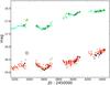 |
Fig. 1 Comparison of V-band OGLE lightcurves of images A & D (points) of QSO 2237 + 0305 with the lightcurves derived from our spectra (diamonds; crosses are used for epochs deviating from the OGLE lightcurves). Error bars (not displayed) are typically of the order of 0.02 mag (A) and 0.04 mag (D). |
We show in Fig. 1a comparison of the V-band lightcurves of images A & D provided by the OGLE collaboration (Udalski et al. 2006) with the lightcurves derived by applying V-band response curve to the spectro-photometric monitoring data. Throughout this paper, we shift the magnitude of image D from the OGLE-III lightcurve by −0.5 mag with respect to the published values to account for different flux calibration of that image in the OGLE-III data (see Paper I for discussion). Although the overall agreement is very good, several epochs identified with an “X” symbol deviate from the OGLE lightcurve. These data are flagged with an asterisk (∗) in Table 1 and we test how they affect our results in Sect. 5.2.
To study how microlensing deforms our spectra and how the broad lines are affected, we use three different techniques that are explained hereafter. First, we apply the multi-component decomposition technique (MCD); i.e., we assume that multiple components cause the quasar emission and measure the flux in these individual components (Sect. 2.1). Second, we use the macro-micro decomposition technique (MmD); i.e., we follow the prescription of Sluse et al. (2007) and Hutsemékers et al. (2010) to decompose the quasar spectrum into a component FM, unaffected by microlensing and another one, FMμ, which is microlensed (Sect. 2.2). Third, we use the narrow band technique (NBD); i.e., we cut the emission lines into different velocity slices and measure the flux in each slice to look for microlensing within the emission line (Sect. 2.3).
Journal of the observations used in this paper.
2.1. The multi-component decomposition (MCD)
Our most comprehensive analysis technique is a multi-component spectral decomposition of the quasar spectrum (MCD). With this technique, we decompose the quasar spectra into the components likely associated with different emission regions (Dietrich et al. 2003). As in Papers I & II, the spectrum is modelled as a sum of three components: i) a power-law for the quasar continuum emission, ii) an empirical iron template, and iii) a sum of Gaussian profiles to model the emission lines. The exact decomposition of each spectrum differs in several respects from the one presented in Papers I & II:
-
First, the quasar emission in image D is corrected for dust reddening produced by the lensing galaxy using the differential extinction values derived in Paper I. We adopt a Cardelli (1989) Milky-way like extinction law with (Rv,Av) = (3.1, 0.2 mag).
-
Because the UV Fe ii+iii template constructed by Vestergaard & Wilkes (2001) from I Zw1 does not perfectly reproduce the Fe ii+iii blended emission observed in QSO 2237 + 0305 , we construct the iron template empirically. In order to take possible intrinsic flux variations and/or systematic errors into account, we proceed independently for data obtained in 2004–2005 (period P1), 2006 (period P2), and 2007 (period P3). This template is constructed iteratively based on the residuals of the fitting procedure. In a first step, we fit only a power-law to the spectra, excluding those regions where Fe ii+iii is known to be significant (Vestergaard & Wilkes 2001) and where there are noticeable quasar broad emission lines. The subsequent fits are performed on the whole quasar spectrum (excluding atmospheric absorption windows), fixing the width and centroid of the quasar emission lines. A new fit is then performed using the residuals as the iron template. The procedure is repeated until a good fit of the whole quasar spectrum is obtained.
-
In order to better reproduce the detailed shape of the C iv and C iii] line profiles, we refine their modelling compared to Paper I by decomposing each line profile into a sum of three Gaussian profiles. The C iv line is composed of two emission (a narrow-component NC and a broad-component BC) and of one absorption component (AC). The faint 1600 Å blend of emission sometimes observed in AGNs, and caused mostly by He ii λ1640, O iii]λ1663 (Fine et al. 2010, and ref. therein), is included by construction in our Fe ii+iii template. To reproduce the C iii] line, we need to use three emission components of increasing width (abbreviated NC, BC, and VBC). With the exception of C iii](VBC), the central wavelength λc of the Gaussians are allowed to vary from epoch to epoch as is the amplitude of each component. Table 2 provides for each image, the central wavelength λc and the FWHM of the different components of the line. The average value and standard deviation between epochs are displayed. When the standard deviation is not displayed, it means that the quantity is fixed for all epochs (see Appendix A for details). Figure 2 shows the C iv and C iii] emission line on 2004−11−14 and the corresponding profile decomposition. As in Paper I, the other emission line profiles (e.g. Al iii, He ii, Si iii], O iii], Mg ii) are fitted with single Gaussian profiles of fixed width.
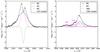 |
Fig. 2 Example of multi component decomposition of the C iv (left) and C iii] (right) line profiles (Sect. 2.1) after continuum and Fe ii subtraction. The narrowest component of the line (NC) is displayed with a dotted-red line, the broad component (BC) with a dashed-blue line, the very broad component (VBC) of C iii] and the absorber in front of C iv are shown in green dot-dashed. The sum of the individual components, corresponding to the line model, is shown with a solid grey line. Characteristics of the components are provided in Table 2. |
Decomposition of the C iv and C iii] emission lines (Average value and scatter between epochs when the parameter is fitted).
The results of the MCD decomposition are shown and discussed in Sect. 3.1. One could suspect that residual flux from the lensing galaxy is included in our empirical FeII template. We tested this possibility by fitting a lens galaxy template (as retrieved from the deconvolution of the 2D spectrum, see Paper I) as an independent component. However, the quasar lightcurves derived in this case strongly disagree with the OGLE lightcurves, indicating that residual contamination of the spectra by the lensing galaxy is not a big issue. Finally, we emphasise that the decomposition of the carbon lines in multiple Gaussians of different widths is empirical and does not necessarily isolate emission lines coming from physically different regions. The adopted naming of the components is based on their width, and is line dependent and internal to this paper. Because of the different decompositions found for the C iv and C iii] lines, comparison between Gaussian components should be performed with care, keeping the actual line widths in mind.
2.2. Macro-micro decomposition (MmD)
This technique, introduced in Sluse et al. (2007) and Hutsemékers et al. (2010) and previously nicknamed FM − FMμ decomposition, allows us to determine the fraction of the quasar emission that is not affected by microlensing independently of any modelling of the quasar spectra. Because spectral differences between lensed images only stem from microlensing (here we correct for differential extinction prior to the decomposition), we can assume that the observed spectrum Fi of image i is the superposition of an emission FM that is only macro-lensed and of another component FMμ, both macro- and micro-lensed. Using pairs of spectra of different lensed images, it is then easy to extract both components FM and FMμ. Defining M = MA/MD (>0) as the macro-magnification ratio between image A and image D, and μ = μA/μD as the microlensing ratio between image A and image D, we have
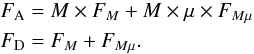 (1)These 2 equations can be rewritten as
 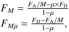 (2)where μ must be chosen to satisfy the positivity constraint FM > 0 and FMμ > 0. For the macro-magnification factor M, we adopt the ratio M = MA/MD = 1.0 provided by the lens model of the Einstein cross performed by Schmidt et al. (1998). The microlensing ratio μ(t,λ) depends on wavelength and time and can be estimated for each epoch based on the ratio of the continuum emission between A & D (Sect. 2.1). Our choice of the continuum flux ratio to derive μ(t,λ) means that we implicitly assume that the emission line and pseudo-continuum emission arise from regions equally or less microlensed than the continuum, in agreement with theoretical expectations. This assumption is also verified a posteriori as our analysis confirms that the continuum emission is also the most microlensed.
2.3. Narrow band technique (NBD)
A simple method of identifying differential microlensing within an emission line is to divide the line into various wavelength bands and calculate the flux ratio FA/FD for each of these bands. For the C iv and C iii] emission, we chose three different wavelength ranges corresponding to the blue wing (BE; −8000 < v < −1500 km s-1), the line core (CE; −1500 < v < 1500 km s-1), and the red wing (RE; 1500 < v < 8000 km s-1) of the line. Before integrating the flux in these ranges, we first remove the continuum and the Fe ii+iii emission from the spectra based on the results of the MCD fit (Sect. 2.1). For the C iii] emission, we also remove the Al iii and Si iii] emission. The central wavelength corresponding to zero velocity is 1549 Å for C iv and 1907.5 Å for C iii].
3. Microlensing variability in the emission lines
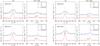 |
Fig. 3 Macro-micro decomposition (MmD) of the C iv (left) and C iii]+Si iii] (right) emission lines obtained from the spectra of images A & D at 4 different epochs. In each panel, the black solid line shows the fraction of the spectrum FMμ affected by microlensing and the red solid line shows the emission FM which is too large to be microlensed. For comparison, we also display the observed spectrum of image D with a dotted blue line and the power-law continuum used to calculate μ(λ,t) with a dashed blue line. |
In Paper I, we reported evidence that the broad emission lines in QSO 2237 + 0305 are significantly microlensed in image A during the monitoring period. In this section, we refine and extend these results (including 2007 data, which were absent from Paper I) using the techniques outlined in Sect. 2. This will allow us to derive lightcurves for the C iv and C iii] emission lines and identify signatures of microlensing.
3.1. C iv and C iii] emission lines
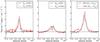 |
Fig. 4 Macro-micro decomposition (MmD) technique applied to the C iv (black) and C iii] (red) emission lines observed on 2006-10-13. Left: fraction of the flux FM non affected by microlensing, Centre: fraction of the line FMμ affected by microlensing, Right: full emission line profile. The intensity of C iii] are multiplied by 2.2 to ease visual comparison between C iv and C iii] profiles. The vertical dashed line indicates the velocity zeropoint corresponding to the systemic redshift. |
First, we investigate how microlensing affects the emission line shape. For this purpose we use the MmD technique (Sect. 2.2). The results of this decomposition for the C iv and C iii] emission are shown in Fig. 3 for four representative epochs. In this figure, we also overplot the continuum model derived from the MCD decomposition and the spectrum of image D. As indicated by Eq. (1), the spectrum of image D should match FMμ in the region of the spectra which are microlensed like the continuum (FMμ = FD when FM = 0). The match between FD and FMμ in the wings of the emission lines reveals that the corresponding emitting region is microlensed as much as the continuum (Fig. 3). It is also apparent that the microlensed fraction of the lines has a broad Gaussian shape with no flux depletion or flat core in the centre (the depletion observed for the C iv emission is caused by the intrinsic absorber). On the other hand, in FM, only a narrow emission line is visible for C iv and C iii]. If we remove the continuum power-law model and Fe ii model prior to the decomposition, and plot the C iii] and C iv lines on a velocity scale (Fig. 4), we find that the decomposed line profiles are rather similar. The remainder of the difference could be caused by Fe ii blended with the C iii] emission, hence not included in our Fe ii template, but may also be real. It is also apparent that the line profile is asymmetric with a stronger blue component and that the C iv line is slightly blueshifted ( ~ 500 km s-1) compared to C iii]. Although comparison between epochs is difficult due to intrinsic variability of the emission lines, we observe that the decomposition remains roughly the same during the period P1 (not shown). During periods P2 and P3, both fractions FM and FMμ of the carbon lines follow the intrinsic brightening of the continuum. We also tentatively see that, during period P3, the line wings appear in FM, indicating that the broadest component is differently microlensed than the continuum at these epochs. We note that the use of a macro-magnification ratio M ~ 0.85, closer to the radio and mid-infrared flux ratios (Falco et al. 1996; Agol et al. 2009; Minezaki et al. 2009), does not change the general features observed in Fig. 3.
The slicing of the emission lines in velocity also allows us to study differential microlensing in the emission lines independently of a model of the line profile. Figure 5 displays the flux measured in the blue wing (BE), red wing (RE), and line core (CE) of the carbon emission lines, using the NBD (Sect. 2.3). Standard error bars are calculated based on the photon noise. Although the error bars are large, we clearly see a difference of about 0.3 mag between the flux ratios measured in the core and the wings of the emission lines. Table 3 shows the average flux ratios for periods P1, P2, P3. Error bars for a period are standard errors calculated based on the dispersion of the data points. The systematic difference observed between the blue and red wings of the C iv profile seems to be mostly caused by an asymmetry of the line’s core. Indeed, the offset between blue and red wing decreases as we increase the width of the central velocity range (not shown). The asymmetry of the FM fraction of the line visible in Fig. 4 supports this finding. When looking to the intrinsic variability of the different bands (i.e. individual lightcurves for images A & D), we observe that the wings vary more significantly on short timescales than does the core of the line.
Average values of magnitude difference ΔmAD as measured in the blue wing (BE), line core (CE), and red wing (RE) of the C iv and C iii] emission lines.
The results of the MCD decomposition are presented in Fig. 6. They broadly agree with the velocity slicing technique (Fig. 5, Table 3). Figure 6 shows that the flux ratio in the full C iii] profile varies weakly over the monitoring interval. A similar flux ratio is measured in C iv and C iii] with evidence of a small increase (ΔmAD closer to 0) in 2007. Figure 6 also confirms that the flux ratio measured in the narrower component of the emission lines is closer to 1 (i.e. the macro-lensed ratio MA/MD), while the flux ratio amounts to nearly 2.5 in the broadest component of the lines (i.e. BC of C iv and VBC of C iii]).
3.2. Other emission lines
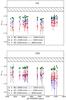 |
Fig. 5 Time dependence of the magnitude difference between images A & D, ΔmAD, as measured in the blue wing (BE; blue diamond), line core (CE; green square) and red wing (RE; red hexagons) of the C iv (top) and C iii] (bottom) emission lines. The shaded area indicates the range of ΔmAD estimated from the macro-model and from MIR measurements. |
An accurate study of the microlensing occurring in the other emission lines is very difficult because of the pseudo-continuum Fe ii+iii in emission blended with these lines. The MmD technique gives qualitative information about microlensing for the other emission lines. Figure 7 shows the FM and FMμ spectra averaged over period P1. We clearly see that not only do C iv and C iii] have their broadest component microlensed, but also Mg ii λ2798, Al ii λ1671, He ii λ1640, and Al iii λ1857. The narrow component of these lines is clearly visible in FM. Interestingly, the Si iii] λ1892 is not microlensed. The absence of microlensed Si iii] emission is also clear in Fig. 3. The bottom panel shows the FeUV template of Vestergaard & Wilkes (2001) convolved with a Gaussian of FWHM ~ 2000 km s-1. Although the iron emission in QSO 2237 + 0305 differs slightly from the Vestergaard & Wilkes (2001) template (Paper I, Sect. 2.1), we clearly see that only the microlensed pseudo-continuum (i.e. emission above the continuum in FMμ) resembles the FeUV emission but, there is no sign of UV iron emission in FM. The pseudo-continuum emission visible in FM at λ > 1920 Å is unlikely to be produced by FeUV because its shape deviates significantly from expectations. The most likely origin(s) of this emission is (are) UV emission from the host galaxy, Balmer continuum emission, and scattered continuum light. Although this feature peaks at about 2200 Å in the quasar rest frame, it is unlikely to be caused by differential extinction in the quasar host galaxy because the light-rays separation between A & D in the host is too small (Falco et al. 1999).
4. Microlensing simulations
In order to derive the size of the regions emitting the carbon lines, we must compare the observed microlensing signal with simulated microlensing lightcurves generated for different source sizes. The strategy we adopt is similar to the one explained in Paper II. Instead of searching for the best simulated lightcurve reproducing the data, we follow a Bayesian scheme for which a probability is associated to each simulated lightcurve. A probability distribution is then derived for each parameter that describes the lightcurve. We provide a description of the crucial steps in the next sections.
4.1. Creating the microlensing pattern
We use the state-of-the-art inverse ray-shooting code developed by Wambsganss (1990, 1999, 2001) to construct micro-magnification maps for images A & D. To create these patterns, the code follows a large number of light-rays (of the order of 1010), from the observer to the source plane, through a field of randomly distributed stars. The surface density of stars and the shear γ at the location of the lensed images are those provided by a macro model of the system. Instead of the surface density, we used the dimensionless quantity κ (the convergence), defined as the ratio between the surface density and the critical density. We use (κ, γ)A = (0.394,0.395) and (κ, γ)D = (0.635, 0.623) (Kochanek 2004). Due to the location of the lensed images behind the bulge of the lens, we assume that 100% of the matter is in the form of compact objects. This assumption is motivated by the results of Kochanek (2004), who demonstrate that the most likely κsmooth = 0 in QSO 2237 + 0305. The mass function of microlenses has little effect on the simulations (Wambsganss 1992; Lewis & Irwin 1995, 1996; Congdon et al. 2007), so we assume identical masses in the simulations. The mass of the microlenses sets the Einstein radius rE. For QSO 2237 + 0305, the Einstein radius projects onto the source plane as  (3)
(3)
where the D are angular diameter distances, and the indices o, l, s refer to observer, lens and source, and M is the mass of microlenses. We create magnification patterns with sidelength of 100 rE and pixel sizes of 0.01 rE. Tracks drawn in such a pattern would provide simulated microlensing lightcurves for one pixel-size source. To simulate lightcurves for other source sizes, we convolve the magnification pattern (after conversion on a linear flux scale) by the intensity profile of the source. As shown by Mortonson et al. (2005), the exact shape of the source intensity profile has little influence on the lightcurve. It instead depends on the characteristic size of the source. For simplicity, we assume a Gaussian profile. A uniform-disc profile is also tested for comparison. We construct magnification maps for 60 different source sizes having characteristic scales (FWHM for the Gaussian and radius for the disc profile) in the range 2–1400 pixels (0.02 rE – 14 rE).
4.2. Comparison with the data
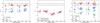 |
Fig. 6 Time variation of the magnitude difference between images A & D, ΔmAD, as measured in the continuum (centre) and in the different components (Fig. 2) of the C iv (left), C iii] (right) emission lines. The shaded area indicates the range of ΔmAD estimated from the macro-model and from MIR measurements. The acronyms NC, BC and VBC refer to the different components (of increasing width) of the C iv & C iii] lines as shown in Fig. 2. |
The patterns created in Sect. 4.1 are used to extract simulated microlensing lightcurves to be compared to the data. Two data sets are used, the OGLE data of QSO 2237 + 0305 (Udalski et al. 2006), which provide well-sampled V-band lightcurves of the continuum variations and our spectrophotometric lightcurves presented in Sect. 2. To study the microlensing signal, we have to get rid of intrinsic variations. This is done by calculating the difference lightcurves between images A & D. Similarly, the simulated microlensing signal is obtained by taking the differences between the simulated tracks for images A & D. The parameters that characterise a simulated microlensing track are the starting coordinates in the magnification patterns ( ,
,  ), the track position angle (θA, θD), and the track length. Because the extracted track is compared to a lightcurve obtained over a given time range, the track length corresponds to the transverse velocity of the source expressed in rE per Julian day. As in Paper II, we assume that the velocity is the same for the trajectories in A & D and the track orientation θA = θD. To account for the roughly orthogonal shears in A & D (Witt & Mao 1994), we rotate the magnification map of D by 90° prior to the track extraction. The difference of the magnitude between track A and track D should, on average, be equal to the one of the macro-model. Like other authors, we account for the uncertainty on the amount of differential extinction between A & D and on the macro-model flux ratio by allowing for a magnitude offset m0 between the simulated lightcurves extracted for A and D. The other parameters characterising the lightcurves are the convergence and shear (κ, γ) fixed in Sect. 4.1. Physical quantities (source size and velocity) are proportional to the mass of microlenses as M1/2.
To build a representative ensemble of lightcurves that is compatible with the data, we followed a four-step strategy similar to the one described in Paper II, in Anguita et al. (2008) and in Kochanek (2004): 1) we pick a set of starting values for the parameters defining the tracks in A & D and vary them to minimise the χ2 between the simulated lightcurve and the OGLE lightcurve; 2) we repeat step 1 to get a representative ensemble of 10000 tracks and good coverage of the parameter space; 3) each track estimated in step 2 is computed for other source sizes, and the agreement with the BLR lightcurve is quantified using a χ2-type merit function; 4) the χ2 estimated in steps (2) and (3) are summed up and used to calculate a likelihood distribution for any track parameter. A summary of the technical details regarding microlensing simulations is given in Appendix B. An example of a good simulated lightcurve fitting the data is shown in Fig. 8. In the next subsection, we explain how we derive probability distributions for the quantities of interest.
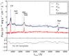 |
Fig. 7 Top: macro-micro decomposition (MmD) applied to the spectra of images A & D averaged over period P1. The black solid line shows the fraction of the spectrum FMμ affected by microlensing, and the red solid line shows the emission FM, which is too large to be microlensed. For comparison, we also display the observed spectrum of image D with a dotted-blue line and the power-law continuum of D with a dashed black line. Bottom: Fe ii+iii template from Vestergaard & Wilkes (2001) convolved with a Gaussian of FWHM = 2000 km s-1. |
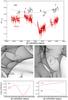 |
Fig. 8 Top: example of a good track fitting the differential lightcurve ΔmAD observed for the C iv broad line and for the continuum. Centre: corresponding tracks (solid line) in the microlensing pattern of image A (left) and D (right). The large circle represents the C iv source size and the small one the continuum. Bottom: track corresponding to the continuum emission (red solid line) and to the C iv emitting region (dashed grey line) for image A (left) and D (right). |
4.3. Probability distribution
The probability of a trajectory j, defined by the set of parameters  ) (where we drop the index j for legibility,
  and
and  refer to the source size of the continuum and of the line) given the data D is, according to Bayes theorem:
  (4)
(4)
where n is the total number of trajectories in the library, L(D | pj) is a likelihood estimator of the data D given the parameters pj and  and P(Vj) are the priors on the continuum source size and velocity respectively. Only the prior on
  and on V appear in Eq. (4) because we use an uniform prior on the other (nuisance) parameters. The prior is required because we have a non uniform sampling of . The prior is related to the density of trajectories as a function of
  given our source sampling in 60 different bins. If falls in the bin b of width lb, then we have P(Rs,j) ∝ lb. The velocity prior P(Vj) is identical to the one used in Anguita et al. (2008). It is based on previous studies by Gil-Merino et al. (2005), which suggest that the net transverse velocity is lower than 0.001 rE/jd (at 90% confidence level). This corresponds to v < 660 km s-1 in the lens plane ( ~ 6000 km s-1 in the source plane) for M ~ 0.1 M⊙, in agreement with the velocity prior used by Kochanek (2004) and Poindexter & Kochanek (2010a).
As explained in Kochanek (2004), the use of the standard likelihood estimator L(D | pj) = exp(−χ2(pj)/2) can lead to misleading results because it is very sensitive to the accuracy of the error bars and to change of the χ2 induced by possible outliers. To circumvent this problem, we follow Kochanek (2004) and use the following likelihood estimator:
![Mathematical equation: \begin{equation} L(D|p_j) = \Gamma\left[\frac{n_{\rm d.o.f.}-2}{2}, \frac{\chi^2(p_j)}{2}\right], \end{equation}](/articles/aa/full_html/2011/04/aa16110-10/aa16110-10-eq120.png) (5)
(5)
where Γ is the incomplete gamma function, and  is the sum of the χ2 obtained when fitting the OGLE data and emission line lightcurves (steps 2 & 3 in Sect. 4.2).
5. Inferences of the quasar structure
In this section, we present the results of our microlensing simulations and discuss them in light of the phenomenological study of the emission lines in A & D. First, we discuss the domain of validity of our simulations and the meaning of the BLR size estimated with our method. Second, we derive the size of the continuum and of the BLR for C iv and C iii]. Third, we compare our results to the radius (BLR)-luminosity relation derived from reverberation mapping. Fourth, we derive the black hole mass of QSO 2237 + 0305 using the virial theorem and compare it to black hole mass derived from the accretion disc size. Finally, we discuss the consequences of our analysis for the BLR structure of QSO 2237 + 0305.
5.1. Caveat
In microlensing simulations, we represent the projected BLR with a face-on disc having a Gaussian or a uniform intensity. The exact intensity profile should not affect our estimate of the size (Mortonson et al. 2005), but the sizes retrieved are only robust if the BLR actually has a morphology that is disc-like when projected on the plane of the sky. This corresponds to the case of a spherically symmetric BLR geometry or of an axi-symmetric geometry with the axis roughly pointing towards us. Since the microlensing signal remains nearly unchanged for sources with ellipticity e = 1 − q < 0.3 (Fluke & Webster 1999; Congdon et al. 2007), our simulations should also be valid for disc-like sources inclined by up to φ ~ 45° with respect to the line of sight. This means that inclination may affect our size estimates by a factor  . Although the exact geometry of the BLR is unknown, there are several lines of evidence that QSO 2237 + 0305 is seen close to face-on. Firstly, QSO 2237 + 0305 is a Type 1 AGN with a flat radio spectrum (α = −0.18, Falco et al. 1996), indicating that the source is seen nearly face-on. Second, the analysis of the microlens-induced continuum flux variations by Poindexter & Kochanek (2010b) show that the inclination of the accretion disc is < 45° at 68.3% confidence level. Third, the C iv line shows only a small blueshift that can be interpreted as evidence that the BLR is seen face-on (Richards et al. 2002).
If the BLR has a disc-like morphology, the projected emission should take place in a ring-like1 region (with an inner radius Rin and outer radius Rout) rather than in a uniform disc as assumed here. The effect of such a “hole” in the BLR emission has been studied by Fluke & Webster (1999), who show that the microlensing lightcurve would be significantly affected only for Rin > 0.5 Rout. Since the BLR is commonly assumed to have Rout > 10 Rin (e.g. Murray & Chiang 1995; Collin & Huré 2001; Borguet & Hutsemékers 2010), we do not consider this geometrical issue.
5.2. Absolute and relative size of the continuum and the BLR
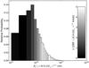 |
Fig. 9 Probability distribution for the half-light radius of continuum emission in QSO 2237 + 0305, colour-coded as a function of the average (lens plane) velocity of the tracks in a given bin. |
The V-band OGLE lightcurve is associated with emission arising mostly from the quasar continuum. The probability distribution of the continuum source size derived from our microlensing study of that lightcurve (Sect. 4) is displayed in Fig. 9. In this figure, we also show the average velocity of the tracks in each source size bin on a colour-coded scale. We see that the source size and the velocity are strongly correlated as expected from the source size/velocity degeneracy (e.g. Kochanek 2004, Paper II). When we consider a uniform prior on the velocity (not shown), we find that by imposing m0, the average difference of magnitude between A & D lightcurves, and the macro-model expectation to be equal, we exclude very high velocities (v > 0.005rE/jd). For the velocity range allowed by the Gil-Merino et al. (2005) velocity prior, the same distributions of m0 are found regardless of what velocity bin is considered. The median half-light radius of the continuum we derive from our simulations is  cm (2.5 × 1015 cm
  cm at 68.3% confidence level, M = 0.3 M⊙) for a Gaussian profile, and
  cm (3.2 × 1015 cm <
  cm at 68.3% confidence level, M = 0.3 M⊙) for a uniform disc. Table 4 compares our measurements with the results of Kochanek (2004, KOC04), Anguita et al. (2008), Paper II, and Poindexter & Kochanek (2010b). The half-light radius (R1/2) allows the comparison of sizes derived with various intensity profiles. We see that our results are compatible with all other works.
The probability distributions of the half-light radius measured for the C iv and C iii] emission lines (using a Gaussian source light profile) are displayed in Fig. 10. Reasonably good fits are obtained for all the line components. However, the quality of the best fits tends to be poorer for the broadest line component (typical reduced χ2 ~ 2). The poorer fits were obtained for the very broad component of the C iii] line that had best reduced χ2 ~ 4. This suggests that our error bars on the flux ratio are underestimated (by a factor ~  ) when measured in the broadest line components. This is expected since the flux in these components of the emission lines are more prone to measurement errors in the MCD decomposition. Our results are, however, robust in the sense that they remain unchanged when the error bars are increased by this factor. Median half-light radius and 68.3% confidence intervals are provided in Table 5 for both Gaussian and uniform-disc intensity profiles of the BLR. These sizes are independent of the intensity profile used for the continuum emission. These results confirm that the most compact region of the quasar is also the one emitting the broadest components of the lines.
While the absolute source sizes derived above depend on the mass of the microlenses, the relative size of the continuum and the BLR are independent of the mass of microlenses. Table 6 displays the ratio between the emission line and the continuum half-light radius size  (assuming the same source profile for the continuum and BLR) at 68.3% confidence for the different components of the BLR identified in Sect. 2.1. We can see that the region emitting the broadest components of the C iv and of the C iii] lines (i.e. C iv BC and C iii] VBC) are about 4 times larger than the region emitting the V-band continuum. In contrast, the narrowest component of the emission lines arises from a region that is typically 25 times larger than the continuum.
We notice that the radius of the extreme-UV continuum ionising the carbon lines (typically λ < 500 Å) is expected to be much smaller than the V-band continuum, with a dependence of the size on wavelength as R ∝ λξ (Paper II and ref. therein). For a standard accretion disc model, ξ = 4/3, implying that the UV ionising continuum is more than 7 times smaller than the OGLE-V band continuum.
Finally, we note that the results of Tables 5 and 6 are not sensitive to possible outliers in our BLR lightcurves. We essentially retrieve the same results when the points inconsistent with the OGLE lightcurve (i.e. those which are marked with a “ × ” in Fig. 1) are excluded. Similar results, but affected by larger error bars, are also obtained if we do not consider the 2007 data.
 |
Fig. 10 Probability distribution for the size of the C iv (top) and C iii] (bottom) broad emission lines. Measurements for the region emitting the C iv & C iii] full emission line profiles (thick black lines, TOT) and for their components NC, BC, and VBC (in order of increasing FWHM, cf. Fig. 2), are presented. |
Half-light radius of the line emitting region  (in
(in  cm) for a Gaussian (G) and a uniform disc (D) intensity profile.
Ratio of size of the BLR to continuum region for Gaussian (G) and uniform disc (D) source profiles.
5.3. C iv radius-luminosity relationship
In this section, we compare our microlensing-based estimate of the C iv emission line (Sect. 5.2) with the radius(BLR)-luminosity relationship (hereafter RBLR − L) derived with the reverberation mapping technique (Sect. 1.2). The RBLR − L relationship for C iv has only been obtained for six objects (Peterson et al. 2005; Kaspi et al. 2007). The luminosity used in this relationship is commonly Lλ(1350 Å). Unfortunately, the latter is out of our spectral range. Instead we use λ Lλ(1450 Å) = 1045.53 erg/s (Assef et al. 2010), which has been shown to be equivalent to Lλ(1350 Å) (Fig. 4 of Vestergaard & Peterson 2006). This luminosity estimate, directly measured on our spectra, is corrected for macro-magnification and line-of-sight Galactic extinction. The macro-magnification is correct within a factor 2 (Witt & Mao 1994). Because the lensed images are located behind the bulge of the galaxy, it is reasonable to assume that the absolute extinction due to the lens is < 1.0 mag. The finite slit width of 0.6″ and seeing ~ 0.6″ may lead to underestimating the total flux by a factor up to 2. This leads to an uncertainty factor of 4 on λ Lλ(1450 Å). The C iv size has been derived to be  =
=  light-days (Table 5). Figure 11 shows the RBLR-L diagram that includes our measurement for QSO 2237 + 0305 and the analytical relation derived by Kaspi et al. (2007) for their so-called “FITEXY” fit. Although the reverberation-mapping size may differ from the half-light radius by a factor up to a few depending on the geometry and density of the BLR gas, we find remarkably good agreement with the R-Lα relationship.
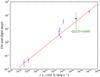 |
Fig. 11 RC iv-L diagram combining reverberation mapping measurement of RC iv (“ × ” symbol, Peterson et al. 2005; Kaspi et al. 2007) and our microlensing-based size for QSO 2237 + 0305. The solid line is the analytical fit to the reverberation mapping data from Kaspi et al. (2007), which has a slope α = 0.52. |
5.4. Black hole mass estimates
The BLR size we derive from microlensing can be used to estimate a black hole mass using the virial theorem:
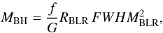 (6)
(6)
where f = 1 is a geometric factor, which encodes assumptions regarding the BLR geometry (e.g. Vestergaard & Peterson 2006; Collin et al. 2006), calibrated from the results of Onken2 et al. (2004). Using FWHMC iv = 3960 ± 180 km s-1 (Assef et al. 2010), we derive  . Consistent measurements, but generally affected by larger error bars, are derived using the other broad components of the emission lines. Hereafter we refer to this black hole mass estimate as
  . As we argued earlier, inclination with respect to the line of sight may reduce RBLR by
  .
.
Our estimate of may be uncertain by a factor of a few because of the variation of f from object to object. A value of f higher than our fiducial value f = 1.0 may be expected for axisymmetric geometry of the BLR seen nearly face-on. The study of several plausible theoretical models of the BLR allowed Collin et al. (2006) to show that inclination of axisymmetric BLR models may noticeably increase f. Observationally, Decarli3 et al. (2008) find f in the range [0.5, 10], with higher values (f > 4) only for objects with FWHM < 4000 km s-1.
The use of the virial theorem to derive MBH based on the C iv line is still debated. For this line, non gravitational effects, such as obscuration and radiation pressure, are probably affecting the C iv profile (Baskin & Laor 2005; Marziani et al. 2006). Obscuration, if present, should lead to underestimating FWHM(C iv) and therefore to overestimating the . The effect of radiation pressure might be subtler. While Marconi et al. (2008) argue that radiation pressure implies an underestimate of MBH, recent calculations of Netzer & Marziani (2010) show that orbits of BLR clouds are affected by radiation pressure in such a way that the product RBLR FWHM2 (and therefore MBH) will vary by at most 25% owing to radiation pressure. Our finding of roughly similar MBH for different components of the line, emitted in regions differently affected by radiation pressure, further supports the idea that MBH in QSO 2237 + 0305 is not strongly biased by nongravitational effects.
A black hole mass estimate can also be derived from the size of the accretion disc. In the accretion disc theory, the radius Rλ which the disc temperature equals the photon energy, kT = hc/λrest is given by the expression (Poindexter & Kochanek 2010b)
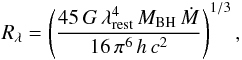 (7)
(7)
where MBH is the black hole mass and Ṁ is the accretion rate. Rewriting this expression for the black hole mass, we get
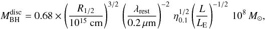 (8)where 0.1 η0.1 = η = L/(Ṁc2) is the radiative efficiency of the accretion disc, R1/2 = 2.44 Rλ the half-light radius of a Shakura-Sunyaev accretion disc model, and L/LE the luminosity in units of Eddington luminosity. Using the accretion disc half-light radius cm (Sect. 5.2), we get
  (2.7
(2.7 at 68.3% confidence) if we assume that L = LE and η = 0.1. Unfortunately,
  is also prone to systematic errors and depends strongly on the exact temperature profile of the disc. The black hole mass derived with this method assumes a temperature profile T ∝ R − ξ′ with ξ′ = 3/4 (Shakura & Sunyaev 1973). A different value of ξ′ in the range [0.5, 1] may lead to higher/lower by a factor as large as ~ 5 (e.g. Poindexter & Kochanek 2010b). The is thus more uncertain and less accurate than .
By comparing the isotropic luminosity L = 4.0 × 1046 erg/s of QSO 2237 + 0305 (Agol et al. 2009) to the Eddington luminosity LE = 1.38 × 1038 MBH/M⊙ erg/s, we derive a black hole mass  , consistent with and .
5.5. The structure of the BLR
Based on the MCD decomposition of the spectra, we have shown that the C iv and C iii] lines can be decomposed into two (resp. three) components of increasing width (Fig. 2). The possibility that these line components correspond to physically distinct regions in the BLR has been discussed by several authors (e.g. Brotherton et al. 1994b; Marziani et al. 2010) but remains debated. The variable amount of microlensing in these components allows us to shed new light on this scenario.
The differential microlensing lightcurves observed for the Gaussian components of the emission line (Fig. 6) are essentially flat, even when a substantial microlensing signal is observed in the continuum. They also show an increasing microlensing effect in the broadest line components. Our simulations show that it is possible to reproduce both the continuum and BLR lightcurves by only changing the source size. We clearly find that the most compact regions have the broadest emission. This excludes BLR models for which the width of the emission line is proportional to the size of the emitting region. Our results are compatible with a variation in the BLR size with FWHM-2 as expected if the emitting regions are virialised. This arises in various geometries, i.e., for a spherically isotropic BLR, a Keplerian disc, or a disc+wind model similar to one proposed by Murray & Chiang (1995, 1997).
The other techniques we used to analyse the spectra provide additional evidence that the BLR of C iv and C iii] is composed of several regions. The “narrow-band” technique (Sect. 2.3) reveals that ΔmAD is closer to the macro model value (i.e., ΔmAD ~ −0.1 ± 0.1) in the core of the emission lines than in the wings. But even in the central 200 km s-1 part of the line, we find ΔmAD ~ −0.6 mag, indicating that there is microlensed flux in the core of the line. The MmD technique (Sect. 2.2) provides more clues to the origin of this flux. The shape of FMμ for the carbon lines smoothly increases from the base to the line centre, and is compatible with a single-peak profile. The lack of “accretion disc-like” profile with a flatter or depleted core (see e.g. Bon et al. 2009) does not exclude a disc-like geometry of the BLR because disc emission can also produce single-peaked profiles (Robinson 1995; Murray & Chiang 1997; Down et al. 2010). The MmD supports the use of a Gaussian to empirically decompose the emission lines with the MCD technique and a composite model of the BLR formed by at least 2 different regions.
Clues to the physical conditions occurring in these regions should come from the flux ratios measured between lines. A detailed analysis, however, needs very high signal-to-noise measurements (based e.g. on an average spectrum of QSO 2237 + 0305 ), proper account of Galactic reddening, and detailed photo-ionisation models. This is beyond the scope of this paper and will be devoted to a future publication. We do, however, mention several features already visible in our spectrum that should provide interesting constraints on photo-ionisation models. First, there is no broad Si iii] emission. The ratio Si iii]/C iii] is very sensitive to the electronic density (Keenan et al. 1987; Aoki & Yoshida 1999). The absence of Si iii] in the broad component of the emission indicates that the electronic density ne in the region emitting the broad component of C iii] is lesser than in the region emitting the narrow portion of the lines. Second, there is no clear narrow Fe ii+iii emission, suggesting that the latter arises from the inner part of the BLR or from a very compact region. This contrasts with microlensing observed in the lensed quasar RXJ 1131–1231 (Sluse et al. 2007) where narrow and broad emission were found for the “optical” Fe ii+iii emission (λ ∈ [3000,5000] Å), since the UV Fe ii is poorly covered by the spectra in that system. Third, the ratio C iii]/C iv is found to be nearly the same in the broad and narrow components of the line (Fig. 4). This advocates for a similar ionisation parameter U in these two regions (Mushotzky & Ferland 1984), which is a priori surprising since U should vary with the distance. In their decomposition of the emission lines based on the principal component analysis technique, Brotherton et al. (1994b) faced a similar problem and found that C iii]/C iv measured for the narrow part of the line (their so-called intermediate line region) was too large by an order of magnitude compared to photo-ionisation models. We speculate that metallicity and optically thick/thin nature of the BLR gas are likely to play important roles in reproducing these ratios (Snedden & Gaskell 1999).
Small differences between the C iv and C iii] line profiles are visible in the total line profile (Fig. 4). The C iii] profile peaks nearly at the systemic redshift and is rather symmetric, while the C iv line shows a low blueshift and an excess of emission in the blue (i.e. blue asymmetry), in agreement with previous studies (Brotherton et al. 1994a). Figure 4 shows that these differences are visible in the narrow component of the line. On the other hand, the very broad component of these lines is slightly asymmetric for both lines, showing again a blue excess but a more greater one for C iv. Because the intrinsic absorber is superimposed on the C iv profile, it is hard to assess whether the broadest component of the profile is in fact blueshifted as is the narrow one. Finally, we mention that the core of the carbon lines varies less than the base of the line, in agreement with the finding of Wilhite (2006) based on a large sample of SDSS quasars. This finding is consistent with the above arguments showing that the broadest part of the line arises from a region closer to the continuum.
6. Conclusions
For the first time, we have derived the size of the broad line region in QSO 2237 + 0305 based on spectrophotometric monitoring data and consisting of 39 different epochs obtained between Oct. 2004 and Dec. 2007. To reach this goal, we measured differential lightcurves between images A & D for the C iv and C iii] broad emission lines and compared them to microlensing simulations. This led to determining the half-light radius of the C iv emitting region: RC iv ~ 66 lt-days (19 lt-days < RC iv < 176 lt-days at 68.3% confidence), in very good agreement with the RBLR − L relation derived from reverberation mapping (Kaspi et al. 2007). The size we derived for C iii] is RC iii] ~ 49 lt-days (14 lt-days < RC iii] < 154 lt-days at 68.3% confidence), compatible with the size estimated for the region emitting C iv.
Thanks to the variable amount of microlensing observed within a given emission line, we can also derive information on the structure of the broad line region. Differential lightcurves obtained for various velocity slices of the C iv and C iii] lines show that the wings of the lines are more microlensed than the core, indicating that the former arise in a more compact region. This finding is confirmed by two other techniques. The first one demonstrates that a broad and single-peaked fraction of the emission line is microlensed, while a narrower fraction is unaffected by microlensing. This technique also suggests a slightly different structure for the C iv and C iii] emission regions, with the narrow C iv emission blueshifted with respect to the systemic redshift. The second technique assumes that the emission lines can be decomposed into a sum of Gaussian components. The C iv is separated into a narrow (FWHM ~ 2600 km s-1) and a broad (FWHM ~ 6300 km s-1) component. In order to reproduce the small differences between the C iv and C iii] lines, we need three Gaussian profiles (FWHM ~ 1550, 3400, 8550 km s-1) to reproduce the latter. The lightcurves derived for these components are essentially flat and show that microlensing is more important when the FWHM increases. Although the individual Gaussian line components do not necessarily isolate individual emission regions, we find that these lightcurves are compatible with the continuum lightcurves, provided only the size of the emission region is modified. This allows us to derive a half-light radius for the regions emitting these components, as well as for their size relative to the continuum. The radii are consistent with the virial hypothesis and a radius that varies as FWHM-2. Using the virial theorem, we derived a black hole mass MBH ~ 2.0 × 10⁸ M⊙ (0.5 × 10⁸ M⊙ < MBH < 5.4 × 10⁸ M⊙ at 68.3% confidence).
Our analysis supports the findings by other authors (Brotherton et al. 1994a; Marziani et al. 2010) that the regions emitting the C iv and C iii] lines are composed of at least two spatially distinct components, one emitting the narrow core of the line and another, more compact, emitting a broadest component. The broad (resp. narrow) component of the C iv and C iii] lines do not have exactly the same profiles. The flux ratio C iii]/C iv is very similar when measured in the broad and in the narrow components of the lines. This suggests that the ionisation parameter U is nearly the same in the two regions, a surprising result since the narrow components are found to arise in regions that are several times larger than the broad components. Other lines observed in our spectra seem to arise from a least two components: Mg ii λ2798, Al ii λ1671, He ii λ1640, Al iii λ1857. The situation is different for Si iii] λ1892, which does not show emission from a broad component, which is indicative of a smaller electronic density ne in the region emitting the broadest part of the emission lines. On the other hand, we detect broad microlensed Fe ii+iii but no “extended” emission. This suggests that FeUV is produced in the inner part of the BLR or in a very compact region. Obtaining spectrophotometric monitoring data in the near-infrared where Balmer lines are detectable would be very useful for constraining photoionisation models and comparing the microlensing signal in Balmer (e.g. H β), high ionisation (e.g. C iv), and Feopt lines.
We demonstrated that the spectrophotometric monitoring of microlensing in a lensed quasar is a powerful technique for probing the inner regions of quasars, measuring the size of the broad line region, and infering its structure. More work is still needed to take full advantage of the method, but our results are very promising. Several improvements are possible to increase the accuracy of our size measurements and better characterise the BLR structure. First, microlensing simulations reproducing the signal in more than 2 lensed images should allow one to narrow the final probability distribution on the source size. Second, the implementation of spectral fitting using Markov-Chain Monte-Carlo should allow a more appropriate estimate of the error bars and more advanced modelling of the individual spectral components. Third, a fully coherent scheme should be developed to consistently model the emission line shape and the corresponding source intensity profile used in the simulation. These improvement will be the subject of a future work.
In the case of emission coming from a spherical shell, the projected profile may also look ring-like, but emission should also arise from the central part of the disc.
Onken et al. derive f = 5.5 but using σ2 instead of FWHM2 in the virial relation. The corresponding value of f when using the FWHM is f = 1.
Decarli et al. use a different definition of f: fthispaper= .
.
Acknowledgments
We thank B. Borguet for useful discussions, and the referee, T. Boroson, for valuable suggestions. D.S. acknowledges support from the Humboldt Foundation. This project is partially supported by the Swiss National Science Foundation (SNSF).
References
- Abajas, C., Mediavilla, E., Muñoz, J. A., et al. 2002, ApJ, 576, 640 [NASA ADS] [CrossRef] [Google Scholar]
- Abajas, C., Mediavilla, E., Muñoz, J. A., Gómez-Álvarez, P., & Gil-Merino, R. 2007, ApJ, 658, 748 [NASA ADS] [CrossRef] [Google Scholar]
- Agol, E., Gogarten, S. M., Gorjian, V., & Kimball, A. 2009, ApJ, 697, 1010 [NASA ADS] [CrossRef] [Google Scholar]
- Anguita, T., Schmidt, R. W., Turner, E. L., et al. 2008, A&A, 480, 327 [NASA ADS] [CrossRef] [EDP Sciences] [Google Scholar]
- Aoki, K., & Yoshida, M. 1999, ASPC, 162, 385 [Google Scholar]
- Assef, R. J., Denney, K. D., Kochanek, C. S., et al. 2010, ApJ, submitted [arXiV:1009.1145v1] [Google Scholar]
- Bachev, R., Marziani, P., Sulentic, J. W., et al. 2004, ApJ, 617, 171 [NASA ADS] [CrossRef] [Google Scholar]
- Baskin, A., & Laor, A. 2004, MNRAS, 350, L31 [NASA ADS] [CrossRef] [Google Scholar]
- Baskin, A., & Laor, A. 2005, MNRAS, 356, 1029 [NASA ADS] [CrossRef] [Google Scholar]
- Bentz, M. C., Peterson, B. M., Pogge, R. W., Vestergaard, M., & Onken, C. A. 2006, ApJ, 644, 133 [NASA ADS] [CrossRef] [Google Scholar]
- Bentz, M. C., Walsh, J. L., & Barth, A. J. 2009, ApJ, 705, 199 [NASA ADS] [CrossRef] [Google Scholar]
- Bentz, M. C., Horne, K., Barth, A. J., et al. 2010, ApJ, 720, L46 [NASA ADS] [CrossRef] [Google Scholar]
- Bon, E., Popović, L. Č., Gavrilović, N., Mura, G. L., & Mediavilla, E. 2009, MNRAS, 400, 924 [NASA ADS] [CrossRef] [Google Scholar]
- Borguet, B., & Hutsemékers, D. 2010, A&A, 515, 22 [Google Scholar]
- Boroson, T. A., & Green, R. F. 1992, ApJS, 80, 109 [NASA ADS] [CrossRef] [Google Scholar]
- Brotherton, M. S., Wills, B. J., Steidel, C. C., & Sargent, W. L. W. 1994a, ApJ, 423, 131 [NASA ADS] [CrossRef] [Google Scholar]
- Brotherton, M. S., Wills, B. J., Francis, P. J., & Steidel, C. C. 1994b, ApJ, 430, 495 [NASA ADS] [CrossRef] [Google Scholar]
- Cardelli, J. A., Clayton, G. C., & Mathis, J. S. 1989, ApJ, 345, 245 [NASA ADS] [CrossRef] [Google Scholar]
- Chen, K., & Halpern, J. P. 1989, ApJ, 344, 115 [NASA ADS] [CrossRef] [Google Scholar]
- Clavel, J., Reichert, G. A., Alloin, D., et al. 1991, ApJ, 366, 64 [NASA ADS] [CrossRef] [Google Scholar]
- Collin, S., & Huré, J.-M. 2001, A&A, 372, 50 [NASA ADS] [CrossRef] [EDP Sciences] [Google Scholar]
- Collin, S., Kawaguchi, T., Peterson, B. M., & Vestergaard, M. 2006, A&A, 456, 75 [NASA ADS] [CrossRef] [EDP Sciences] [Google Scholar]
- Courbin, F., Magain, P., Kirkove, M., & Sohy, S. 2000, ApJ, 529, 1136 [NASA ADS] [CrossRef] [Google Scholar]
- Congdon, A. B., Keeton, C. R., & Osmer, S. J. 2007, MNRAS, 376, 263 [NASA ADS] [CrossRef] [Google Scholar]
- Corbin, M. R. 1990, ApJ, 347, 346 [NASA ADS] [CrossRef] [Google Scholar]
- Corbin, M. R. 1995, ApJ, 447, 496 [NASA ADS] [CrossRef] [Google Scholar]
- Corbett, E., Robinson, A., Axon, D. J., Young, S., & Hough, J. H. 1998, MNRAS, 296, 721 [NASA ADS] [CrossRef] [Google Scholar]
- Decarli, R., Labita, M., Treves, A., & Falomo, R. 2008, MNRAS, 387, 1237 [NASA ADS] [CrossRef] [Google Scholar]
- Denney, K. D., Peterson, B. M., Pogge, R. W., et al. 2009, ApJ, 704, L80 [NASA ADS] [CrossRef] [Google Scholar]
- Dietrich, M., Hamann, F., Appenzeller, I., et al. 2003, ApJ, 596, 817 [NASA ADS] [CrossRef] [Google Scholar]
- Down, E. J., Rawlings, S., Sivia, D. S., & Baker, J. C. 2010, MNRAS, 401, 633 [NASA ADS] [CrossRef] [Google Scholar]
- Eigenbrod, A., Courbin, F., Sluse, D., et al. 2007, A&A, 480, 647 (Paper I) [Google Scholar]
- Eigenbrod, A., Courbin, F., Meylan, G., et al. 2008, A&A, 490, 933 (Paper II) [NASA ADS] [CrossRef] [EDP Sciences] [Google Scholar]
- Elvis, M. 2000, ApJ, 545, 63 [NASA ADS] [CrossRef] [Google Scholar]
- Falco, E. E., Lehar, J., Perley, R. A., et al. 1996, AJ, 112, 897 [NASA ADS] [CrossRef] [Google Scholar]
- Falco, E. E., Impey, C. D., Kochanek, C. S., et al. 1999, ApJ, 523, 617 [NASA ADS] [CrossRef] [Google Scholar]
- Fine, S., Croom, S. M., Bland-Hawthorn, J., et al. 2010, MNRAS, 409, 591 [NASA ADS] [CrossRef] [Google Scholar]
- Francis, P. J., Hewett, P. C., Foltz, C. B., & Chaffee, F. H. 1992, ApJ, 398, 476 [NASA ADS] [CrossRef] [Google Scholar]
- Fluke, C. J., & Webster, R. L. 1999, MNRAS, 302, 68 [NASA ADS] [CrossRef] [Google Scholar]
- Gaskell, C. M. ApJ, 263, 79 [Google Scholar]
- Gaskell, C. M., Klimek, E. S., & Nazarova, L. S. 2007, ApJ, submitted [arXiv:0711.1025] [Google Scholar]
- Gaskell, C. M. 2009, NewAR, 53, 140 [Google Scholar]
- Gaskell, C. M. 2010a, IAUS, 267, 203 [NASA ADS] [Google Scholar]
- Gaskell, C. M. 2010b, ApJ, submitted [arXiv:1008.1057] [Google Scholar]
- Gil-Merino, R., Wambsganss, J., Goicoechea, L. J., & Lewis, G. F. 2005, A&A, 432, 83 [NASA ADS] [CrossRef] [EDP Sciences] [Google Scholar]
- Gültekin, K., Richstone, D. O., Gebhardt, K., et al. 2009, ApJ, 698, 198 [NASA ADS] [CrossRef] [Google Scholar]
- Horne, K., Peterson, B. M., Collier, S. J., & Netzer, H. 2004, PASP, 116, 465 [NASA ADS] [CrossRef] [Google Scholar]
- Hintzen, P., Maran, S. P., Michalitsianos, A. G., et al. 1990, AJ, 99, 45 [NASA ADS] [CrossRef] [Google Scholar]
- Huchra, J., Gorenstein, M., Kent, S., et al. 1985, AJ, 90, 691 [NASA ADS] [CrossRef] [Google Scholar]
- Hutsemékers, D., Surdej, J., & van Drom, E. 1994, Ap&SS, 216, 361 [NASA ADS] [CrossRef] [Google Scholar]
- Hutsemékers, D., Borguet, B., Sluse, D., Riaud, P., & Anguita, T. 2010, A&A, 519, 103 [Google Scholar]
- Hu, C., Wang, J., Ho, L. C., et al. 2008, ApJ, 683, L115 [NASA ADS] [CrossRef] [Google Scholar]
- Jarvis, M. J., & McLure, R. J. 2006, MNRAS, 369, 182 [NASA ADS] [CrossRef] [Google Scholar]
- Kollatschny, W., & Dietrich, M. 1996, A&A, 314, 43 [NASA ADS] [Google Scholar]
- Kaspi, S., Maoz, D., & Netzer, H. 2005, ApJ, 629, 61 [NASA ADS] [CrossRef] [Google Scholar]
- Kaspi, S., Brandt, W. N., Maoz, D., et al. 2007, ApJ, 659, 997 [NASA ADS] [CrossRef] [Google Scholar]
- Kayser, R., Refsdal, S., & Stabell, R. 1986, A&A, 166, 36 [NASA ADS] [Google Scholar]
- Keenan, F. P., Kingston, A. E., & Dufton, P. L. 1987, MNRAS, 225, 859 [NASA ADS] [Google Scholar]
- Kochanek, C. S. 2004, ApJ, 605, 58 [Google Scholar]
- Krolik, J. H., Horne, K., Kallman, T. R., et al. 1991, ApJ, 371, 541 [NASA ADS] [CrossRef] [Google Scholar]
- Laor, A. 2007, ASPC, 373, 384 [NASA ADS] [Google Scholar]
- Lewis, G. F., & Irwin, M. J. 1995, MNRAS, 276, 103 [NASA ADS] [Google Scholar]
- Lewis, G. F., & Irwin, M. J. 1996, MNRAS, 283, 225 [NASA ADS] [Google Scholar]
- Lewis, G. F., & Belle, K. E. 1998, MNRAS, 297, 69 [NASA ADS] [CrossRef] [Google Scholar]
- Lewis, G. F., & Ibata, R. A. 2004, MNRAS, 348, 24 [NASA ADS] [CrossRef] [Google Scholar]
- Lewis, G. F., & Ibata, R. A. 2006, MNRAS, 367, 1217 [NASA ADS] [CrossRef] [Google Scholar]
- Magain, P., Courbin, F., & Sohy, S. 1998, ApJ, 494, 452 [Google Scholar]
- Marconi, A., Axon, D. J., Maiolino, R., et al. 2008, ApJ, 678, 693 [NASA ADS] [CrossRef] [Google Scholar]
- Marziani, P., Sulentic, J. W., Dultzin-Hacyan, D., Calvani, M., & Moles, M. 1996, ApJS, 104, 37 [Google Scholar]
- Marziani, P., Dultzin-Hacyan, D., & Sulentic, J. W. 2006, New Developments in Black Hole Research, ed. P. V. Kreitler, 123 [Google Scholar]
- Marziani, P., Sulentic, J. W., Negrete, C. A., et al. 2010, MNRAS, 409, 1033 [NASA ADS] [CrossRef] [Google Scholar]
- McLure, R. J., & Dunlop, J. S. 2002, MNRAS, 331, 795 [NASA ADS] [CrossRef] [Google Scholar]
- Metcalf, R. B., Moustakas, L. A., Bunker, A. J., et al. 2004, ApJ, 607, 43 [Google Scholar]
- Morgan, C. W., Kochanek, C. S., Morgan, N. D., & Falco, E. E. 2010, ApJ, 712, 1129 [NASA ADS] [CrossRef] [Google Scholar]
- Mortonson, M. J., Schechter, P. L., & Wambsganss, J. 2005, ApJ, 628, 594 [NASA ADS] [CrossRef] [Google Scholar]
- Motta, V., Mediavilla, E., Muñoz, J. A., & Falco, E. 2004, ApJ, 613, 86 [NASA ADS] [CrossRef] [Google Scholar]
- Minezaki, T., Chiba, M., Kashikawa, N., Inoue, K. T., & Kataza, H. 2009, ApJ, 697, 610 [NASA ADS] [CrossRef] [Google Scholar]
- Mushotzky, R., & Ferland, G. J. 1984, ApJ, 278, 558 [NASA ADS] [CrossRef] [Google Scholar]
- Murray, N., & Chiang, J. 1995, ApJ, 454, 105 [Google Scholar]
- Murray, N., & Chiang, J. 1997, ApJ, 474, 91 [NASA ADS] [CrossRef] [Google Scholar]
- Netzer, H. 2003, ApJ, 583, L5 [NASA ADS] [CrossRef] [Google Scholar]
- Netzer, H., & Marziani, P. 2010, ApJ, 724, 318 [NASA ADS] [CrossRef] [Google Scholar]
- Onken, C. A., Ferrarese, L., Merritt, D., et al. 2004, ApJ, 615, 645 [NASA ADS] [CrossRef] [Google Scholar]
- Peterson, B. M., Balonek, T. J., Barker, E. S., et al. 1991, ApJ, 368, 119 [NASA ADS] [CrossRef] [Google Scholar]
- Peterson, B. M., Bentz, M. C., Desroches, L.-B., et al. 2005, ApJ, 632, 799 (+Erratum) [NASA ADS] [CrossRef] [Google Scholar]
- Poindexter, S., & Kochanek, C. S. 2010a, ApJ, 712, 658 [NASA ADS] [CrossRef] [Google Scholar]
- Poindexter, S., & Kochanek, C. S. 2010b, ApJ, 712, 668 [NASA ADS] [CrossRef] [Google Scholar]
- Popović, L. Č. 2006, SerAJ, 173, 1 [NASA ADS] [Google Scholar]
- Popović, L. Č., Mediavilla, E. G., Jovanović, P., & Muñoz, J. A. 2003, A&A, 398, 975 [NASA ADS] [CrossRef] [EDP Sciences] [Google Scholar]
- Popović, L. Č., Mediavilla, E., Bon, E., & Ilić, D. 2004 A&A, 423, 909 [Google Scholar]
- Rice, M. S., Martini, P., & Greene, J. E. 2006, ApJ, 636, 654 [NASA ADS] [CrossRef] [Google Scholar]
- Richards, G. T., Van den Berk, D. E., Reichard, T. A., et al. 2002, AJ, 124, 1 [NASA ADS] [CrossRef] [Google Scholar]
- Richards, G. T., Keeton, C. R., Pindor, B., et al. 2004, ApJ, 610, 679 [NASA ADS] [CrossRef] [Google Scholar]
- Risaliti, G., Salvati, M., & Marconi, A. 2010, MNRAS, in press [arXiv:1010.2037] [Google Scholar]
- Rix, H. W., Schneider, D. P., & Bahcall, J. N. 1992, AJ, 104, 959 [NASA ADS] [CrossRef] [Google Scholar]
- Robinson, A. 1995, MNRAS, 272, 647 [NASA ADS] [Google Scholar]
- Schmidt, R., Webster, R. L., & Lewis, G. F. 1998, MNRAS, 295, 488 [NASA ADS] [CrossRef] [Google Scholar]
- Schneider, P., & Wambsganss, J. 1990, A&A, 237, 42 [NASA ADS] [Google Scholar]
- Shakura, N. I., & Sunyaev, R. A. 1973, A&A, 24, 337 [NASA ADS] [Google Scholar]
- Sluse, D., Claeskens, J.-F., Hutsemékers, D., et al. 2007, A&A, 468, 885 [NASA ADS] [CrossRef] [EDP Sciences] [Google Scholar]
- Sluse, D., Claeskens, J.-F., Hutsemékers, D., et al. 2008, RMxAC, 32, 83 [NASA ADS] [Google Scholar]
- Snedden, S. A., & Gaskell, M. C. 1999, ApJ, 521, 91 [Google Scholar]
- Smith, J. E., Robinson, A., Young, S., Axon, D. J., & Corbett, E. A. 2005, MNRAS, 359, 846 [NASA ADS] [CrossRef] [Google Scholar]
- Sulentic, J. W., & Marziani, P. 1999, ApJ, 518, L9 [NASA ADS] [CrossRef] [Google Scholar]
- Sulentic, J. W., Marziani, P., Zwitter, T., & Calvani, M. 1995, ApJ, 438, L1 [NASA ADS] [CrossRef] [Google Scholar]
- Sulentic, J. W., Marziani, P., & Dultzin-Hacyan, D. 2000, ARA&A, 38, 521 [NASA ADS] [CrossRef] [Google Scholar]
- Udalski, A., Szymański, M., Kubiak, M., et al. 2006, AcA, 56, 293 [Google Scholar]
- Van den Berk, D. E., Richards, G. T., Bauer, A., et al. 2001, AJ, 122, 549 [NASA ADS] [CrossRef] [Google Scholar]
- Vestergaard, M., & Wilkes, B. J. 2001, ApJS, 134, 1 [NASA ADS] [CrossRef] [Google Scholar]
- Vestergaard, M., & Peterson, B. M. 2006, ApJ, 641, 689 [NASA ADS] [CrossRef] [Google Scholar]
- Vestergaard, M., Wilkes, B. J., & Barthel, P. D. 2000, ApJ, 538, L103 [NASA ADS] [CrossRef] [Google Scholar]
- Wambsganss, J. 1990, Ph.D. Thesis, Munich University [Google Scholar]
- Wambsganss, J. 1992, ApJ, 386, 19 [NASA ADS] [CrossRef] [Google Scholar]
- Wambsganss, J. 1999 , JCoAM, 109, 353 [Google Scholar]
- Wambsganss, J. 2001, PASA, 18, 207 [NASA ADS] [CrossRef] [Google Scholar]
- Wambsganss, J., & Paczyński, B. 1991, AJ, 102, 864 [NASA ADS] [CrossRef] [Google Scholar]
- Wambsganss, J., & Paczyński, B. 1994, AJ, 108, 1156 [NASA ADS] [CrossRef] [Google Scholar]
- Wayth, R. B., O’Dowd, M., & Webster, R. L. 2005, MNRAS, 359, 561 [NASA ADS] [CrossRef] [Google Scholar]
- Wills, B. J., Brotherton, M. S., Fang, D., Steidel, C. C., & Sargent, W. L. W. 1993, ApJ, 415, 563 [NASA ADS] [CrossRef] [Google Scholar]
- Wilhite, B. C., Van den Berk, D. E., Brunner, R. J., & Brinkmann, J. V. 2006, ApJ, 641, 78 [NASA ADS] [CrossRef] [Google Scholar]
- Witt, H. J., & Mao, S. 1994, ApJ, 429, 66 [NASA ADS] [CrossRef] [Google Scholar]
- Whittle, M. 1985, MNRAS, 213, 33 [NASA ADS] [Google Scholar]
- Young, S., Axon, D. J., Robinson, A., Hough, J. H., & Smith, J. E. 2007, Nature, 450, 74 [NASA ADS] [CrossRef] [PubMed] [Google Scholar]
- Yee, H. K. C., & De Robertis, M. M. 1991, ApJ, 381, 386 [NASA ADS] [CrossRef] [Google Scholar]
- Zamfir, S., Sulentic, J. W., & Marziani, P. 2008, MNRAS, 387, 856 [NASA ADS] [CrossRef] [Google Scholar]
- Zhu, L., Zhang, S. N., & Tang, S. 2009, ApJ, 700, 1173 [NASA ADS] [CrossRef] [Google Scholar]
Appendix A: Averaged emission line profile
We explain here how we construct an averaged emission line profile and how we use it to choose a reasonable multi-Gaussian decomposition of the broad emission lines. Following the prescriptions of the multi-component decomposition described in Sect. 2.1, we are able to subtract the quasar pseudo-continuum emission (including the Fe ii+iii emission) from the quasar spectra. This procedure leads to a spectrum containing only the broad emission lines. Then, we normalize their flux and compare the line profiles averaged over periods P1, P2, and P3. This procedure reveals that the profile of the C iii] emission line basically remains unchanged over the whole monitoring period. In contrast, there is evidence of a small change in the C iv line profile between 2005 and 2007. The high signal- to-noise emission line spectra of C iii] and C iv are then fitted with a sum of 3 Gaussian-line profiles. For C iii], we find that the best fit is obtained with a narrow emission component with FWHM = 1545 km s-1, an intermediate emission component FWHM = 3400 km s-1, and a broad component with FWHM = 8548 km s-1. For C iv, the emission line is well fitted with only two emission components with FWHM ~ 2570 km s-1 and FWHM ~ 6150 km s-1. The absorption component is also fitted with an FWHM ~ 1250 km s-1 for P1 and P2 and FWHM ~ 900 km s-1 for P3. The difference in width of the absorption comes from the increased resolution of the spectra obtained during period P3. Higher resolution spectra (Hintzen et al. 1990; Yee & De Robertis 1991) show that the C iv absorption system is composed of at least two different absorption clouds associated with the quasar. Narrow absorption systems are also present in front of C iii] emission (Motta et al. 2004), but they do not appear as significant features in our spectra and are therefore not part of our modelling.
If we now compare the decomposition of the line profile in images A & D, we find that the width of the individual Gaussian profiles are similar but not their relative intensities, as already suggested by the analysis in Paper I. During our fitting procedure, we assume that the FWHM of the Gaussian components are identical for A & D, except for C iv(BC) and C iv(AC). The widths are also fixed to the fiducial values derived here.
Appendix B: Microlensing fit
We provide here the technical details regarding the comparison of the simulated tracks with data. The following source sizes are considered: 2, 4, 8, 12, 16, 20, 24, 28, 32, 36, 40, 44, 48, 52, 56, 60, 70, 80, 90, 100, 110, 120, 130, 140, 150, 160, 170, 180, 190, 200, 240, 280, 320, 360, 400, 440, 480, 520, 560, 600, 640, 680, 720, 760, 800, 840, 880, 920, 960, 1000, 1040, 1080, 1120, 1160, 1200, 1240, 1280, 1320, 1360, and 1400 pixels. For each of the 60 source sizes Rs, we simulate 10000 pairs of lightcurves for both images A & D by tracing source trajectories across the magnification patterns. Bilinear interpolation is used for the track extraction. Each track is characterised by the set of parameters described in Sect. 4.2: p = (Rs,V,m0,θ,x0,A,x0,D,M). Each simulated difference lightcurve  is then compared to the data D = Δmk by measuring the goodness of fit with a χ2 statistic,
 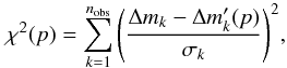 (B.1)where σk are the uncertainties of the data and nobs is the number of data points. For OGLE data, we use those obtained between modified julian day (i.e. JD-2 450 000) 3100 and 4500, and we bin the data points obtained the same night, which leads to nobs = 181. The error σk is the quadratic sum of the photometric error σOGLE provided by OGLE, of the standard deviation σbin between binned points, and of the systematic underestimation of the error σsys of the OGLE data. The error σsys is estimated using a polynomial fitting of the difference lightcurves (see Paper II) and is estimated to be σsys = 0.05 mag. The data points corresponding to the BLR lightcurve have been described in Sect. 3.1.
The brute force approach, which consists in randomly picking track parameters and estimating a χ2 is very inefficient in getting even a few tracks reproducing the data unless a large amount of computing time is available. To overcome this problem, we follow the procedure explained in Paper II and, for each set of random parameters we have generated, we optimise the 6 parameters (m0,xA,xD,θ) with a χ2 based minimisation algorithm using a Levenberg-Marquardt least-square routine. Contrary to what was done in Paper II, we do not optimise the track velocity to avoid possible bias on the velocity distribution induced by the minimisation routine. In addition, we windowed the magnification map in such a way that the starting point of a track is always more then one track length away from the border of the map. Our final library of tracks fitting OGLE data contains 6 × 10⁵ tracks (10 000 track per source size) with a χ2/nobs < 8.5.
The only parameter that is varied to compare the tracks of our library to the BLR lightcurves is the source size Rs. As explained in Sect. 4.2, we extract, for each track of our library (step 2), the same track in the 59 other magnification maps corresponding to the 59 source sizes. We then search for the best source size using a minimisation routine and calculate tracks for arbitrary source sizes (in the range 0.01–14 rE) by means of a quadratic spline interpolation between different source sizes.
All Tables
Decomposition of the C iv and C iii] emission lines (Average value and scatter between epochs when the parameter is fitted).
Average values of magnitude difference ΔmAD as measured in the blue wing (BE), line core (CE), and red wing (RE) of the C iv and C iii] emission lines.
Half-light radius of the line emitting region (in cm) for a Gaussian (G) and a uniform disc (D) intensity profile.
Ratio of size of the BLR to continuum region for Gaussian (G) and uniform disc (D) source profiles.
All Figures
|
Fig. 1 Comparison of V-band OGLE lightcurves of images A & D (points) of QSO 2237 + 0305 with the lightcurves derived from our spectra (diamonds; crosses are used for epochs deviating from the OGLE lightcurves). Error bars (not displayed) are typically of the order of 0.02 mag (A) and 0.04 mag (D). |
| In the text | |
|
Fig. 2 Example of multi component decomposition of the C iv (left) and C iii] (right) line profiles (Sect. 2.1) after continuum and Fe ii subtraction. The narrowest component of the line (NC) is displayed with a dotted-red line, the broad component (BC) with a dashed-blue line, the very broad component (VBC) of C iii] and the absorber in front of C iv are shown in green dot-dashed. The sum of the individual components, corresponding to the line model, is shown with a solid grey line. Characteristics of the components are provided in Table 2. |
| In the text | |
|
Fig. 3 Macro-micro decomposition (MmD) of the C iv (left) and C iii]+Si iii] (right) emission lines obtained from the spectra of images A & D at 4 different epochs. In each panel, the black solid line shows the fraction of the spectrum FMμ affected by microlensing and the red solid line shows the emission FM which is too large to be microlensed. For comparison, we also display the observed spectrum of image D with a dotted blue line and the power-law continuum used to calculate μ(λ,t) with a dashed blue line. |
| In the text | |
|
Fig. 4 Macro-micro decomposition (MmD) technique applied to the C iv (black) and C iii] (red) emission lines observed on 2006-10-13. Left: fraction of the flux FM non affected by microlensing, Centre: fraction of the line FMμ affected by microlensing, Right: full emission line profile. The intensity of C iii] are multiplied by 2.2 to ease visual comparison between C iv and C iii] profiles. The vertical dashed line indicates the velocity zeropoint corresponding to the systemic redshift. |
| In the text | |
|
Fig. 5 Time dependence of the magnitude difference between images A & D, ΔmAD, as measured in the blue wing (BE; blue diamond), line core (CE; green square) and red wing (RE; red hexagons) of the C iv (top) and C iii] (bottom) emission lines. The shaded area indicates the range of ΔmAD estimated from the macro-model and from MIR measurements. |
| In the text | |
|
Fig. 6 Time variation of the magnitude difference between images A & D, ΔmAD, as measured in the continuum (centre) and in the different components (Fig. 2) of the C iv (left), C iii] (right) emission lines. The shaded area indicates the range of ΔmAD estimated from the macro-model and from MIR measurements. The acronyms NC, BC and VBC refer to the different components (of increasing width) of the C iv & C iii] lines as shown in Fig. 2. |
| In the text | |
|
Fig. 7 Top: macro-micro decomposition (MmD) applied to the spectra of images A & D averaged over period P1. The black solid line shows the fraction of the spectrum FMμ affected by microlensing, and the red solid line shows the emission FM, which is too large to be microlensed. For comparison, we also display the observed spectrum of image D with a dotted-blue line and the power-law continuum of D with a dashed black line. Bottom: Fe ii+iii template from Vestergaard & Wilkes (2001) convolved with a Gaussian of FWHM = 2000 km s-1. |
| In the text | |
|
Fig. 8 Top: example of a good track fitting the differential lightcurve ΔmAD observed for the C iv broad line and for the continuum. Centre: corresponding tracks (solid line) in the microlensing pattern of image A (left) and D (right). The large circle represents the C iv source size and the small one the continuum. Bottom: track corresponding to the continuum emission (red solid line) and to the C iv emitting region (dashed grey line) for image A (left) and D (right). |
| In the text | |
|
Fig. 9 Probability distribution for the half-light radius of continuum emission in QSO 2237 + 0305, colour-coded as a function of the average (lens plane) velocity of the tracks in a given bin. |
| In the text | |
|
Fig. 10 Probability distribution for the size of the C iv (top) and C iii] (bottom) broad emission lines. Measurements for the region emitting the C iv & C iii] full emission line profiles (thick black lines, TOT) and for their components NC, BC, and VBC (in order of increasing FWHM, cf. Fig. 2), are presented. |
| In the text | |
|
Fig. 11 RC iv-L diagram combining reverberation mapping measurement of RC iv (“ × ” symbol, Peterson et al. 2005; Kaspi et al. 2007) and our microlensing-based size for QSO 2237 + 0305. The solid line is the analytical fit to the reverberation mapping data from Kaspi et al. (2007), which has a slope α = 0.52. |
| In the text | |
Current usage metrics show cumulative count of Article Views (full-text article views including HTML views, PDF and ePub downloads, according to the available data) and Abstracts Views on Vision4Press platform.
Data correspond to usage on the plateform after 2015. The current usage metrics is available 48-96 hours after online publication and is updated daily on week days.
Initial download of the metrics may take a while.