| Issue |
A&A
Volume 526, February 2011
|
|
|---|---|---|
| Article Number | A120 | |
| Number of page(s) | 7 | |
| Section | The Sun | |
| DOI | https://doi.org/10.1051/0004-6361/201015582 | |
| Published online | 10 January 2011 | |
Intensity contrast from MHD simulations and HINODE observations
1
Astrophysics Group, Imperial College London,
SW7 2AZ,
UK
e-mail: This email address is being protected from spambots. You need JavaScript enabled to view it.
2
Max-Planck-Institut für Sonnensystemforschung,
Max-Planck-Strasse 2,
37191
Katlenburg-Lindau,
Germany
3
School of Space Research, Kyung Hee University,
Yongin, Gyeonggi
446-701,
Korea
4
Sterrekundig Instituut, Utrecht University,
Postbus 80 000, 3508 TA
Utrecht, The
Netherlands
Received: 13 August 2010
Accepted: 8 November 2010
Abstract
Context. Changes in the solar surface area, which is covered by small-scale magnetic elements, are thought to cause long-term changes in the solar spectral irradiance, which are important for determining the impact on Earth’s climate.
Aims. To study the effect of small-scale magnetic elements on the total and spectral irradiance, we derive their contrasts from 3-D MHD simulations of the solar atmosphere. These calculations are necessary because measurements of small-scale flux tube contrasts are confined to a few wavelengths and affected by scattered light and instrument defocus, even for space observations.
Methods. To test the contrast calculations, we compare rms contrasts from simulations with those obtained with the broad-band filter imager mounted on the Solar Optical Telescope (SOT) onboard the Hinode satellite and also analyse centre-to-limb variations (CLV). The 3-D MHD simulations include the interaction between convection and magnetic flux tubes. They are performed by assuming non-grey radiative transfer and using the MURaM code. The simulations have an average vertical magnetic field of 0 G, 50 G, and 200 G. Emergent intensities are calculated with the spectral synthesis code ATLAS9 and are convolved with a theoretical point-spread function to account for the properties of the observations’ optical system.
Results. We find reasonable agreement between simulated and observed intensity distributions in the visible continuum bands. Agreement is poorer for the CN and G-bands. The analysis of the simulations uncovers a potentially more realistic centre-to-limb behaviour than calculations based on 1-D model atmospheres.
Conclusions. We conclude that starting from 3-D MHD simulations represents a powerful approach to obtaining intensity contrasts for a wide wavelength coverage and different positions across on the solar disk. This also paves the way for future calculations of facular and network contrast as a function of magnetic fluxes.
Key words: Sun: surface magnetism / Sun: activity
© ESO, 2011
1. Introduction
Understanding the variability of the Earth’s atmosphere requires being able to distinguish between anthropogenic and natural drivers of climate change. One important natural driver influencing our climate is solar irradiance (i.e. the radiative flux of the Sun, measured above the Earth’s atmosphere) and in particular its variation. Changes in the Sun’s total irradiance influence the amount of energy reaching the Earth. In addition, changes in the solar spectral irradiance, i.e. the changes in the Sun’s brightness at a certain wavelength, influence the chemistry of the Earth’s upper atmosphere (e.g. Haigh 2007). Finally, the heliospheric magnetic field (Potgieter 1998; Simpson 1998) shields the Earth from Galactic cosmic rays, which have been proposed to increase cloud cover (Marsh & Svensmark 2000). The solar surface magnetic field, which manifests itself in, e.g., sunspots, faculae, and the network is able to reproduce solar irradiance variations on solar-cycle timescales (e.g. Krivova et al. 2003; Wenzler et al. 2005, 2006). For longer timescales, however, there is considerable uncertainty. While sunspots and faculae dominate the solar irradiance changes on timescales of days to weeks, the small-scale magnetic elements in the network are considered to be the main cause of long-term changes in the solar irradiance (Foukal & Lean 1988; Solanki & Fligge 2002). The contribution of sunspots to irradiance changes is well understood and produces a decrease in solar irradiance. The contribution from faculae and in particular smaller-scale magnetic elements composing the photospheric network increases the solar irradiance and is still being investigated. In particular, the spectral response is poorly understood. To achieve a clearer understanding of irradiance variations, it is important to study the centre-to-limb variation and the wavelength dependence of the emergent intensity.
The direct measurement of the solar network contrast in order to determine the impact of these small-scale magnetic elements remains difficult, because it is (even for space instruments) affected by the instrument’s aperture, scattered light, instrument defocus, etc. and is in addition limited to a few wavelengths. Therefore, we calculate emergent intensities from 3-D simulations of solar magneto-convection and calculate the intensity variation between brighter and darker features to compare the simulations with observations. Filtergrams with a high and constant spatial resolution can be obtained with the broad-band filter imager (BFI) mounted on the Solar Optical Telescope (SOT, Tsuneta et al. 2008; Ichimoto et al. 2008; Suematsu et al. 2008; Shimizu et al. 2008) onboard the HINODE spacecraft (Kosugi et al. 2007). To compare measured and simulated granulation contrasts, we convolved the simulations with the point-spread function (PSF) of the observation’s optical system (Mathew et al. 2009) to take into account its effects. Here, we analyse simulations with different average magnetic fields, in contrast to previous studies that mainly included non-magnetic simulations: Danilovic et al. (2008) analysed Hinode/SP data and compared the intensity contrast of a Hinode/SP continuum map of the quiet Sun with predictions of non-magnetic simulations, and Wedemeyer-Böhm & van der Voort (2009) compared Hinode/SOT observations to non-magnetic simulations to determine the continuum intensity distributions of the solar photosphere.
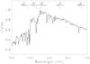 |
Fig. 1 Spectrum of the visible wavelength regions at disk centre (calculated with ATLAS9 for the non-magnetic simulation) with the positions of the five Hinode filters indicated. |
The paper is organised as follows: the observations are described in Sect. 2, the simulations, the intensity synthesis originating from them, and the subsequent convolution are introduced in Sect. 3. We compare the Hinode/SOT/BFI observations with the simulations in Sect. 4 (in terms of histograms and rms contrasts) and also discuss the statistical aspects of this comparison. The centre-to-limb behaviour of the intensity contrast in our simulations is analysed in Sect. 5.
2. Observations
We consider two different datasets from the Hinode Solar Optical Telescope (SOT):
Dataset I was recorded during the Mercury transit on 8 November 2006 (21:38:31–21:39:16 UT) in five wavelength filters: CN bandhead (“CN”, 388.3 nm), G band (“GB”, 430.5 nm), blue continuum (“BC”, 450.4 nm), green continuum (“GC”, 555.0 nm), and red continuum (“RC”, 668.4 nm) (Fig. 1). The observed region corresponded to the quiet Sun. The full observed Hinode image covers approximately 223 × 112 arcsec and the pixel size is 0.05 arcsec. The heliocentric coordinates at the centre of the image were (0,–419), corresponding to a limb angle of μ = 0.9, where cos θ = μ and θ is the the angle between the line of sight and the line through the centre of the Sun. The dark correction and flat fielding were done with SSW-IDL routines. The Mercury transit allowed the calculation of the point-spread function (PSF) with high confidence. Details of the calculation of the PSF and this particular data set can be found in Mathew et al. (2009).
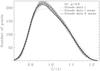 |
Fig. 2 Comparison of Hinode datasets I (Mercury transit) and II for the green continuum wavelength at the limb angle μ = 0.9. For dataset I, we plot 37 histograms where each includes ten random extracts of the whole observed image (grey lines) and the mean histogram (solid line). We overplot the mean of the analogous quantity for dataset II (black dashed line). |
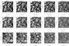 |
Fig. 3 Simulations (original and convolved) and observations in the five Hinode/SOT filters. Top: Original simulation snapshots with an input magnetic field of 50 G. Black: 52% below the mean, white: 68% above the mean value. Middle: Same simulation snapshots convolved with an appropriate point-spread function (PSF). Bottom: Extracts from observed image. The black/white scale for the convolved simulations and the observations is such that black is 33% below the mean, and white is 40% above the mean value. |
Dataset II was recorded on 8 March 2007 (18:02:32–20:51:46 UT) in the same wavelength filters as dataset I. While the quiet Sun was also observed in this observation, the binning was different with a pixel size of 0.10 arcsec. The data were recorded in 12 steps from the east to the west limb, resulting in the availability of data at all limb angles. At each step, the observed image covers approximately a field of view of 223 × 112 arcsec, as in dataset I. For each image, we chose extracts such that their area corresponds to the desired limb angle solely. This allowed us to use dataset II for comparisons with calculations at limb angles from disk centre to the limb. It should be noted that we observed different areas on the Sun at different limb angles whose activity levels might be different.
Dataset I was compared with dataset II at μ = 0.9 to check the validity of the PSF for dataset II. An example is shown in Fig. 2, where we compare histograms for the two datasets in the green continuum (GC). The number of resulting subimages in the two datasets of course differ. For dataset I, we segmented the observed image into 373 sub-images (extracts) of the desired size. Four extracts had to be excluded because of the transit of Mercury. To illustrate the spread in dataset I, we overplot in Fig. 2 (in grey) 37 histograms where each includes ten random extracts of the whole observed image. For dataset II, we have 151 subimages, and, for ease of comparison, we confine ourselves to plotting only the mean histogram over all the 151 histograms of the subimages. For dataset I, the subimages are scaled to the pixel size of the subimages in dataset II, which for the limb angle μ = 0.9 implies that there are 68 × 76 pixels per subimage. The mean histogram of dataset II appears to be a bit wider than that of dataset I, but overall we find good agreement. We follow the procedure outlined in Numerical Recipes (Press et al. 1992) and calculate the χ2 statistic for two binned distributions (with unequal numbers of data points), where Ri is the number of events in bin i for the first data set, and Si the number of events in the same bin i for the second data set 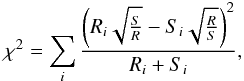 (1)where
 (2)are the respective numbers of data points.
The reduced χ2 value (i.e. the χ2 value divided by the number of degrees of freedom) between the mean of dataset I and dataset II is 0.42, suggesting that they are equivalent within the scatter. With similar results obtained for the other wavelength bands, this justifies the use of the same PSF for both datasets.
For comparison with simulations (described in the next section), an extract (or subimage) of an observation in this work is chosen such that it has the same physical size as one simulation snapshot, which corresponds to approximately 7.5 arcsec × 8.3 arcsec under a limb angle of μ = 0.9. This individual segment can then be directly compared with one simulation in terms of visual appearance, histograms, and contrast, as done in Sect. 4.
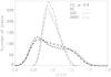 |
Fig. 4 Histograms of the intensity distribution in the original simulation for the GC wavelength at the limb angle μ = 0.9: 0 G (black dotted), 50 G (black dashed), and 200 G (black long dashes). We overplot (in grey) the corresponding histograms for the convolved simulation to illustrate the effect of convolving with the PSF. |
3. Calculations
3.1. MHD simulations
The 3-D MHD simulations were performed using the MURaM code (Vögler et al. 2005) with non-grey radiative transfer using four opacity bins and 24 ray directions to determine the radiative heating/cooling rates (Vögler et al. 2004). On the Sun, the computational box corresponds horizontally to a square of 6 Mm × 6 Mm and has a vertical extension of 1.4 Mm, covering the range between about 500 km above and 900 km below the visible solar surface that is located at an average height of optical depth unity. The cell size of the numerical grid is 20.8 km in the horizontal directions and 14 km in the vertical. We used three simulation runs with initially homogeneous and unipolar vertical magnetic fields of 0 G, 50 G, and 200 G, respectively. Since we wish to study the effect of the surface magnetic field on the radiative output at the surface, we do not prescribe the total radiative surface flux, but rather assume a fixed constant entropy density of the fluid entering the simulation box through the open lower boundary (Vögler 2005). The value of the entropy density has been chosen such that the resulting mean radiative energy flux in the non-magnetic run matches the observed solar value to within 1%. In all three simulations, the total radiative output at the top of the simulation box fluctuates by about ±1% around its mean value in the course of the five-minute oscillations in the box. Each simulation was run for about 150 min of solar time after a statistically stationary state of the magneto-convective system had evolved. For the detailed analysis we then considered ten equidistant snapshots covering about 20 min to suppress the effects of the five-minute oscillations and to reduce the statistical fluctuations. Vögler (2005) used these simulations to study the centre-to-limb variation in the bolometric intensity as a function of the average vertical magnetic field.
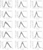 |
Fig. 5 Histograms of the intensity distribution in convolved simulations and in observations for the five Hinode/SOT wavelengths, from top to bottom: 388 nm, 430 nm, 450 nm, 555 nm, and 668 nm. From left to right: Limb angles μ = 0.9, μ = 0.6, μ = 0.3. The histograms for the simulations are shown for three different magnetic fluxes: 0 G (dotted), 50 G (dashed), and 200 G (long dashes). To illustrate the spread in the observations, we overplot histograms of extracts of the whole observed image (grey lines). The black solid line indicates the mean over all observed extracts. Note the different scales in the horizontal axes. |
3.2. Intensities
We calculate the emergent intensities along parallel rays, each passing through a different point of the surface grid of the MHD simulations. Since we are interested in a broad spectral coverage, we use Kurucz’ spectral synthesis code ATLAS9 (Kurucz 1993) (which includes diatomic molecules) with opacity distribution functions (ODFs) on each of those simulated model atmospheres at disk centre and towards the limb. ATLAS9 (as rewritten by Lester) and the ODFs were obtained through CCP7 (Collaborative Computing Project No. 71). The program solves the radiative transfer equations under the assumption of local thermodynamic equilibrium (LTE). The simplification of LTE and the use of ODFs allows us to calculate the whole spectrum from 160 nm to 160 000 nm with a spectral resolution of better than 200 in the visible. However, the HINODE/SOT/BFI filters are narrower than the ATLAS9 resolution bins, and, in addition, the spectra are not calculated at the wavelength centre for the filters, which leads to a comparison at slightly different wavelengths. Furthermore, the CN and GB regions comprise many spectral lines that are only approximated by coarsely resolved ODFs in the ATLAS9 calculation. This may influence the comparison of the simulated intensities with the observations for the CN and GB wavelengths.
For an inclined view away from disk centre, we allow the line of sight to cut through the simulated atmosphere at an angle θ to the surface normal (θ is the heliocentric angle). For our simulation box, this means that we have to interpolate the atmosphere parameters along rays with the respective heliocentric angle.
For comparison with observations, we degraded the simulated images to take into account optical effects. The point-spread functions for the SOT as calculated by Mathew et al. (2009) were used for both dataset I and dataset II, as discussed in Sect. 2.
4. Comparisons of observations with simulations
Here, we compare the resulting intensities from simulations with observations to validate the simulated results. For dataset I at μ = 0.9 with its finer binning, we first inspect the observed and simulated intensity images visually for a qualitative comparison. In a subsequent step, we compare dataset II with the simulations (at all limb angles) in terms of rms contrasts and intensity distributions.
4.1. Simulations versus dataset I: Visual comparison
In this section, we compare observations with original and convolved simulations at a limb angle of μ = 0.9. In Fig. 3 original and convolved MURaM simulation snapshots for 50 G are shown together with the observed image in the respective wavelength filter. The qualitative agreement is good, the granules are of comparable size and the visually perceived contrasts appear to be similar. The occurrence of brighter and darker features is similar and also changes correspondingly for the different wavelength filters. The brightest features can be seen in the CN wavelength. The bright magnetic features that appear for the 50 G (as seen in Fig. 3) and 200 G simulations are not seen for non-magnetic simulations.
4.2. Simulations versus dataset II: rms contrasts and intensity distributions at different limb angles
In Fig. 4, we demonstrate the effect of convolving with the PSF in a more quantitative way. We plot, as an example, the histograms for the green continuum intensity distribution in the original simulation at the limb angle μ = 0.9 for 0 G, 50 G, and 200 G. We overplot (in grey) the corresponding histogram for the convolved simulation as shown in Fig. 5. As expected, the convolved histograms are significantly narrower. For most wavelengths, we find a distribution with a double peak in the unconvolved simulations, which is most prominent in the 50 G simulation and represents both the dark intergranular components (the more prominent peak at I/ ⟨ I ⟩ < 1) and the bright granular components (the weaker peak at I/ ⟨ I ⟩ > 1) (see e.g. Wedemeyer-Böhm & van der Voort (2009) and references therein). After the convolution, the double-peak is smeared out, but important differences between the non-magnetic, 50 G, and 200 G simulations remain, in particular for the visible broadband distributions (BC, GC, and RC).
Figure 5 shows the histograms of the intensity for (all) ten averaged simulation snapshots and for average magnetic fields of 0 G, 50 G, and 200 G. From left to right, we plot histograms for the convolved simulations at the three limb angles μ = 0.9, μ = 0.6, and μ = 0.3 (i.e. from disk centre towards the limb) and for all five Hinode/SOT wavelengths (from top to bottom: CN: 388 nm, GB: 430 nm, BC: 450 nm, GC: 555 nm, RC: 668 nm). We also show the average histograms for the Hinode observations (dataset II, solid black line). We illustrate the spread in the observations by overplotting histograms of extracts of the observed image (grey lines). For ease of comparison, the simulations have been renormalised to cover the same number of points as the observations.
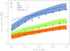 |
Fig. 6 RMS contrasts for the BC, GC, and RC Hinode/SOT wavelengths at the limb angles μ = 0.2−1.0 for the mean over the 0 G simulation snapshots (dotted lines), the 50 G simulation snapshots (dashed line), the 200 G simulation snapshots (long dashes), and the Hinode dataset II observations (diamonds). We show the spread in the ten snapshots of the 50 G simulation and overplot the 1σ error of the Hinode dataset II observations. Overplotted (black crosses) are the Hinode dataset I results at μ = 0.9, which are almost indistinguishable from the dataset II results. |
At the limb angle of μ = 0.9, the agreement between data and simulations is reasonable for all wavelengths. Closer to the limb, at μ = 0.6 and μ = 0.3, the histograms for the simulations in the CN and GB wavelengths do not agree with the measurements. For the three continuum filters, however, the agreement is satisfactory, as the histograms for the simulations all fall within the scatter of the data. None of the simulations precisely match the observed histograms, which leads to high χ2 values. A quantitative comparison and the χ2 analysis are discussed in the next section.
Intensity variations between bright and dark features determine the root-mean-square (rms) contrast, which is the standard deviation divided by the mean value. Figure 6 compares the rms contrasts for the convolved 0 G, 50 G, and 200 G simulations to the resulting rms contrast from the observations at the limb angles μ = 0.2−1.0. For the simulations, these rms contrasts are the averages of rms contrasts for all simulation runs. For the observations, we calculate the rms contrasts for each of the extracts of the observed images, i.e. extracts of similar size as one simulation snapshot, and then average them.
We consider the change in the rms contrast as one moves from weaker to higher magnetic fluxes, as indicated by the dotted, dashed, and long-dashed lines in Fig. 6 for the 0 G, 50 G, and 200 G simulations, respectively. It can be seen that the 200 G rms contrast is not a simple extrapolation of the 0 G and 50 G contrasts. The 0 G and 50 G rms contrasts look very similar, although the 50 G rms contrast falls off a bit more steeply. The 200 G rms contrast shows a much flatter profile with a lower contrast at disk centre and a higher contrast at the limb than the weaker fields. The rms contrasts suggest that the 50 G simulation agrees slightly more closely with the Hinode observations than the 0 G simulation for all wavelengths. Although the 200 G simulation fits the observations better near disk centre (as can also be seen from the χ2 statistic in the next section), its overall behaviour does not represent the one seen in the data. Given that the observations refer to the quiet Sun, this result is unsurprising. The agreement between the contrast as measured from the observations and the simulation for 50 G is good in the visible continuum bands at 450.4 nm (BC), 555.0 nm (GC), and 668.4 nm (RC). The contrasts derived for 388.3 nm (CN) and 430.5 nm (GB) are generally too large. For the 50 G simulation, they can exceed the measured contrasts by up to a factor of 1.5 and 1.3 for CN and GB, respectively, depending on limb angle.
4.3. Statistics for simulations
Although the differences between the simulations with different average magnetic fluxes are less distinct after the convolution, they can still be seen in the histograms in Fig. 5. To find the simulations that agree most closely with the observations, we calculate the value of χ2 according to Eq. (1), where Ri and Si are the number of pixels in intensity bin i for the observations and simulations, respectively. The χ2 values are shown in Fig. 7 for limb angles of μ = 0.2−1.0 and for the five Hinode wavelength filters. As each histogram has 50 bins, i.e., 49 degrees of freedom (d.o.f), we would expect a good fit to have a value of χ2 ≃ 49. This corresponds to a value of approximately one for the reduced χ2 given by  . The grey line in Fig. 7 indicates the level where
  .
.
It turns out that, except at disk centre, none of the simulations fit the CN or G-band observations well. This is not too surprising as we assume LTE in our spectral synthesis calculations, and, furthermore, do not carry out a full line-by-line synthesis, but use ODFs to approximate the opacity in relatively coarse wavelength bins (see Sect. 3). For the blue, green and red continuum bands, the simulations agree reasonably well, though it appears that the 200 G simulation most closely reproduces the positions closer to disk centre, while the 0 G and 50 G simulations show better agreement closer to the limb.
 |
Fig. 7 χ2 values for histograms of convolved simulations as shown in Fig. 5 but for all the limb angles μ = 0.2−1.0. The χ2 values for 0 G, 50 G, and 200 G are represented by dotted, dashed, and long-dashed lines, respectively. The Δχ2 for a confidence level of 99% is 75 for 50 bins. A Δχ2 of 75 is indicated by the solid line on the right of each plot. The grey line at χ2 = 49 indicates the level where |

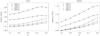 |
Fig. 8 Centre-to-limb variations for the five different Hinode/SOT wavelengths for an average vertical magnetic field of 50 G and 200 G, respectively. Note the different scales of the y-axes. |
We can use contours of equal χ2 to examine whether the convolved intensity distributions derived for different magnetic flux levels are distinguishable, i.e., appear to be drawn from a different underlying population. To this aim, we calculate  , where
  denotes the minimum χ2. In our case of 50 bins, Δχ2 values in excess of 75 suggest a different distribution at a confidence level of 99% (see Press et al. 1992). The 99% confidence levels are indicated by the vertical bars on Fig. 7. They confirm that the intensities calculated for the CN filter are not a good representation of the observations, except near disk centre, where the convolved non-magnetic, 50 G, and 200 G distributions are indistinguishable at the 99% confidence level. In all other bands, the non-magnetic and the 50 G convolved distributions are largely indistinguishable, while the 200 G distributions appear to have significantly different behaviours, in particular towards the limb (see also the right-hand column in Fig. 5). While the 50 G simulation does not represent the best-fit solution at most limb angles, it largely lies within Δχ2 = 75.
5. Intensity contrasts in simulations
The centre-to-limb variation in the emergent intensity varies with wavelength. In the UV, magnetic features are brighter than at other wavelengths. These differences become even stronger near the limb and are therefore crucial for spectral solar irradiance variations. It is generally impossible to reproduce the observed limb behaviour with 1-D model calculations, as they tend to overestimate the limb contrast at extreme limb angles.
In Figure 8, we show the simulated contrasts (i.e. the mean intensity of the ten average magnetic 3-D MHD simulation snapshots compared to the mean quiet Sun (=0 G) intensity) with average vertical magnetic field of 50 G and 200 G as a function of heliocentric position in the five Hinode wavelength filters. As expected, the contrast increases towards the limb and is higher for shorter wavelengths. The result is qualitatively consistent with Fig. 4 in Vögler (2005) if one assumes that the bolometric intensity corresponds roughly to the maximum of the Planck curve. In contrast to 1-D models, the flattening and turnover (e.g. for 50 G at 388 nm and 430 nm) are in closer agreement with measurements of facular contrasts than 1-D calculations (Topka et al. 1997; Unruh et al. 1999; Ortiz et al. 2002).
6. Conclusions and outlook
We have compared simulated and observed intensity distributions in the quiet Sun at a range of limb angles and derived mean contrasts for simulations with average magnetic fields of 0 G, 50 G, and 200 G.
Comparing histograms and rms contrasts of the observations and simulations, we have found that no single simulation reproduces the data for all limb distances and colour bands. The 50 G simulation intensity histograms and rms contrasts agree most closely with the observations near the limb and exhibit an overall similar behaviour. The 200 G simulation, however, reproduces the observations better near disk centre, but does not represent the overall behaviour of the observed rms contrasts.
There may be various reasons for the discrepancy between the data and the simulations. One of these could be the use of LTE in ATLAS9 along with our not calculating spectral lines (which mainly affects the results for CN and GB). In addition, in our dataset we observed different areas of the Sun at various limb angles with potentially differing activity levels. By averaging over a large area, the Hinode histograms represent a de facto mixture of features/magnetic fluxes that we would expect to be reproduced by a combination of the simulations with 0 G/50 G/200 G average magnetic fields. Furthermore, the height of the model atmosphere in our simulation box might be insufficient. As the radiation is produced at increasingly higher layers in the atmosphere as one moves to the solar limb and shorter wavelengths, the computational box might be insufficiently high to encompass enough of the region where the radiation originates. This problem becomes particularly acute for the CN and GB data, because of the presence of strong lines formed particularly high.
The approach presented in this study should allow us to calculate the facular and network contrast not solely as a function of limb angle, but also as a function of magnetic flux. For this purpose, we will calculate magnetograms from MURaM simulations and identify the previously determined emergent intensities with corresponding magnetic fluxes. Depending on our future tests, these facular and network intensities could then be incorporated into irradiance reconstruction models (such as SATIRE; see e.g. Krivova et al. 2003), which would enable us to help improve these models, as well as identify the cause of irradiance variations even more reliably. Of particular interest will be a detailed comparison of the output of MHD simulations with the high-resolution, low-straylight Sunrise observations (Barthol et al. 2010; Solanki et al. 2010), especially those from the SUFI instrument (Gandorfer et al. 2010), which will go beyond just the comparison of rms values at solar disk centre performed in Hirzberger et al. (2010).
Acknowledgments
N.A. acknowledges the SNSF (Swiss National Science Foundation) grant PBEZP2-124350. N.A. and Y.C.U. would also like to acknowledge the support through the NERC SolCli consortium grant (UK) and through ISSI (Switzerland). This work was partially supported by WCU grant No. R31-10016 of the Korean Ministry of Education, Science and Technology. The authors would like to acknowledge Hinode, the Japanese mission, developed and launched by ISAS/JAXA, with NAOJ as domestic partner and NASA and STFC (UK) as international partners. It is operated by these agencies in co-operation with ESA and NSC (Norway).
References
- Barthol, P., Gandorfer, A., Solanki, S. K., et al. 2010, Sol. Phys., in press [Google Scholar]
- Danilovic, S., Gandorfer, A., Lagg, A., et al. 2008, A&A, 484, L17 [NASA ADS] [CrossRef] [EDP Sciences] [Google Scholar]
- Foukal, P., & Lean, J. 1988, ApJ, 328, 347 [NASA ADS] [CrossRef] [Google Scholar]
- Gandorfer, A., Grauf, B., Barthol, P., et al. 2010, Sol. Phys., in press [Google Scholar]
- Haigh, J. D. 2007, Living Rev. Sol. Phys., 4, 2, http://www.livingreviews.org/lrsp-2007-2 [NASA ADS] [Google Scholar]
- Hirzberger, J., Feller, A., Riethmüller, T. L., et al. 2010, ApJ, Lett., 723, L154 [NASA ADS] [CrossRef] [Google Scholar]
- Ichimoto, K., Katsukawa, Y., Tarbell, T., et al. 2008, in First Results From Hinode, ed. S. A. Matthews, J. M. Davis, & L. K. Harra, ASP Conf. Ser., 397, 51 [Google Scholar]
- Kosugi, T., Matsuzaki, K., Sakao, T., et al. 2007, Sol. Phys., 243, 3 [NASA ADS] [CrossRef] [Google Scholar]
- Krivova, N. A., Solanki, S. K., Fligge, M., & Unruh, Y. C. 2003, A&A, 399, L1 [NASA ADS] [CrossRef] [EDP Sciences] [Google Scholar]
- Kurucz, R. L. 1993 (CDROM No. 13) [Google Scholar]
- Marsh, N. D., & Svensmark, H. 2000, Phys. Rev. Lett., 85, 5004 [NASA ADS] [CrossRef] [PubMed] [Google Scholar]
- Mathew, S. K., Zakharov, V., & Solanki, S. K. 2009, A&A, 501, L19 [NASA ADS] [CrossRef] [EDP Sciences] [Google Scholar]
- Ortiz, A., Solanki, S. K., Domingo, V., Fligge, M., & Sanahuja, B. 2002, A&A, 388, 1036 [NASA ADS] [CrossRef] [EDP Sciences] [Google Scholar]
- Potgieter, M. S. 1998, Space Sci. Rev., 83, 147 [NASA ADS] [CrossRef] [Google Scholar]
- Press, W. H., Teukolsky, S. A., Vetterling, W. T., & Flannery, B. P. 1992, Numerical Recipes in C, 2nd edn. (New York: Cambridge University Press) [Google Scholar]
- Shimizu, T., Nagata, S., Tsuneta, S., et al. 2008, Sol. Phys., 249, 221 [NASA ADS] [CrossRef] [Google Scholar]
- Simpson, J. A. 1998, Space Sci. Rev., 83, 7 [NASA ADS] [CrossRef] [Google Scholar]
- Solanki, S. K., & Fligge, M. 2002, Adv. Space Res., 29, 1933 [NASA ADS] [CrossRef] [Google Scholar]
- Solanki, S. K., Barthol, P., Danilovic, S., et al. 2010, ApJ, Lett., in press [Google Scholar]
- Suematsu, Y., Tsuneta, S., Ichimoto, K., et al. 2008, Sol. Phys., 249, 197 [NASA ADS] [CrossRef] [Google Scholar]
- Topka, K. P., Tarbell, T. D., & Title, A. M. 1997, ApJ, 484, 479 [NASA ADS] [CrossRef] [Google Scholar]
- Tsuneta, S., Ichimoto, K., Katsukawa, Y., et al. 2008, Sol. Phys., 249, 167 [NASA ADS] [CrossRef] [Google Scholar]
- Unruh, Y., Solanki, S. K., & Fligge, M. 1999, A&A, 345, 635 [NASA ADS] [Google Scholar]
- Vögler, A. 2005, Mem. Soc. Astron. Ital., 76, 842 [Google Scholar]
- Vögler, A., Bruls, J. H. M. J., & Schüssler, M. 2004, A&A, 421, 741 [NASA ADS] [CrossRef] [EDP Sciences] [Google Scholar]
- Vögler, A., Shelyag, S., Schüssler, M., et al. 2005, A&A, 429, 335 [NASA ADS] [CrossRef] [EDP Sciences] [Google Scholar]
- Wedemeyer-Böhm, S., & van der Voort, L. R. 2009, A&A, 503, 225 [NASA ADS] [CrossRef] [EDP Sciences] [Google Scholar]
- Wenzler, T., Solanki, S. K., & Krivova, N. A. 2005, A&A, 432, 1057 [NASA ADS] [CrossRef] [EDP Sciences] [Google Scholar]
- Wenzler, T., Solanki, S. K., Krivova, N. A., & Fröhlich, C. 2006, A&A, 460, 583 [NASA ADS] [CrossRef] [EDP Sciences] [Google Scholar]
All Figures
|
Fig. 1 Spectrum of the visible wavelength regions at disk centre (calculated with ATLAS9 for the non-magnetic simulation) with the positions of the five Hinode filters indicated. |
| In the text | |
|
Fig. 2 Comparison of Hinode datasets I (Mercury transit) and II for the green continuum wavelength at the limb angle μ = 0.9. For dataset I, we plot 37 histograms where each includes ten random extracts of the whole observed image (grey lines) and the mean histogram (solid line). We overplot the mean of the analogous quantity for dataset II (black dashed line). |
| In the text | |
|
Fig. 3 Simulations (original and convolved) and observations in the five Hinode/SOT filters. Top: Original simulation snapshots with an input magnetic field of 50 G. Black: 52% below the mean, white: 68% above the mean value. Middle: Same simulation snapshots convolved with an appropriate point-spread function (PSF). Bottom: Extracts from observed image. The black/white scale for the convolved simulations and the observations is such that black is 33% below the mean, and white is 40% above the mean value. |
| In the text | |
|
Fig. 4 Histograms of the intensity distribution in the original simulation for the GC wavelength at the limb angle μ = 0.9: 0 G (black dotted), 50 G (black dashed), and 200 G (black long dashes). We overplot (in grey) the corresponding histograms for the convolved simulation to illustrate the effect of convolving with the PSF. |
| In the text | |
|
Fig. 5 Histograms of the intensity distribution in convolved simulations and in observations for the five Hinode/SOT wavelengths, from top to bottom: 388 nm, 430 nm, 450 nm, 555 nm, and 668 nm. From left to right: Limb angles μ = 0.9, μ = 0.6, μ = 0.3. The histograms for the simulations are shown for three different magnetic fluxes: 0 G (dotted), 50 G (dashed), and 200 G (long dashes). To illustrate the spread in the observations, we overplot histograms of extracts of the whole observed image (grey lines). The black solid line indicates the mean over all observed extracts. Note the different scales in the horizontal axes. |
| In the text | |
|
Fig. 6 RMS contrasts for the BC, GC, and RC Hinode/SOT wavelengths at the limb angles μ = 0.2−1.0 for the mean over the 0 G simulation snapshots (dotted lines), the 50 G simulation snapshots (dashed line), the 200 G simulation snapshots (long dashes), and the Hinode dataset II observations (diamonds). We show the spread in the ten snapshots of the 50 G simulation and overplot the 1σ error of the Hinode dataset II observations. Overplotted (black crosses) are the Hinode dataset I results at μ = 0.9, which are almost indistinguishable from the dataset II results. |
| In the text | |
|
Fig. 7 χ2 values for histograms of convolved simulations as shown in Fig. 5 but for all the limb angles μ = 0.2−1.0. The χ2 values for 0 G, 50 G, and 200 G are represented by dotted, dashed, and long-dashed lines, respectively. The Δχ2 for a confidence level of 99% is 75 for 50 bins. A Δχ2 of 75 is indicated by the solid line on the right of each plot. The grey line at χ2 = 49 indicates the level where |
| In the text | |
|
Fig. 8 Centre-to-limb variations for the five different Hinode/SOT wavelengths for an average vertical magnetic field of 50 G and 200 G, respectively. Note the different scales of the y-axes. |
| In the text | |
Current usage metrics show cumulative count of Article Views (full-text article views including HTML views, PDF and ePub downloads, according to the available data) and Abstracts Views on Vision4Press platform.
Data correspond to usage on the plateform after 2015. The current usage metrics is available 48-96 hours after online publication and is updated daily on week days.
Initial download of the metrics may take a while.