| Issue |
A&A
Volume 526, February 2011
|
|
|---|---|---|
| Article Number | A58 | |
| Number of page(s) | 12 | |
| Section | The Sun | |
| DOI | https://doi.org/10.1051/0004-6361/201014369 | |
| Published online | 21 December 2010 | |
A novel technique to measure intensity fluctuations in EUV images and to detect coronal sound waves nearby active regions⋆
1
Interferometrics, Inc.,
Herndon,
VA
20171,
USA
e-mail: This email address is being protected from spambots. You need JavaScript enabled to view it.
2
Max-Planck-Institut für Sonnensystemforschung,
37191
Katlenburg-Lindau,
Germany
3
Naval Research Laboratory, Washington, DC
20375,
USA
4
Praxis, Inc., Alexandria, VA
22303,
USA
Received:
5
March
2010
Accepted:
31
October
2010
Abstract
Context. In the past years, evidence for the existence of outward-moving (Doppler blue-shifted) plasma and slow-mode magneto-acoustic propagating waves in various magnetic field structures (loops in particular) in the solar corona has been found in ultraviolet images and spectra. Yet their origin and possible connection to and importance for the mass and energy supply to the corona and solar wind is still unclear. There has been increasing interest in this problem thanks to the high-resolution observations available from the extreme ultraviolet (EUV) imagers on the Solar TErrestrial RElationships Observatory (STEREO) and the EUV spectrometer on the Hinode mission.
Aims. Flows and waves exist in the corona, and their signatures appear in EUV imaging observations but are extremely difficult to analyse quantitatively because of their weak intensity. Hence, such information is currently available mostly from spectroscopic observations that are restricted in their spatial and temporal coverage. To understand the nature and origin of these fluctuations, imaging observations are essential. Here, we present measurements of the speed of intensity fluctuations observed along apparently open field lines with the Extreme UltraViolet Imagers (EUVI) onboard the STEREO mission. One aim of our paper is to demonstrate that we can make reliable kinematic measurements from these EUV images, thereby complementing and extending the spectroscopic measurements and opening up the full corona for such an analysis. Another aim is to examine the assumptions that lead to flow versus wave interpretation for these fluctuations.
Methods. We have developed a novel image-processing method by fusing well established techniques for the kinematic analysis of coronal mass ejections (CME) with standard wavelet analysis. The power of our method lies with its ability to recover weak intensity fluctuations along individual magnetic structures at any orientation, anywhere within the full solar disk, and using standard synoptic observing sequences (cadence <3 min) without the need for special observation plans.
Results. Using information from both EUVI imagers, we obtained wave phase speeds with values on the order of 60−90 km s-1, compatible with those obtained by other previous measurements. Moreover, we studied the periodicity of the observed fluctuations and established a predominance of a 16-min period, and other periods that seem to be multiples of an underlying 8-min period.
Conclusions. The validation of our analysis technique opens up new possibilities for the study of coronal flows and waves, by extending it to the full disk and to a larger number of coronal structures than has been possible previously. It opens up a new scientific capability for the EUV observations from the recently launched Solar Dynamics Observatory. Here we clearly establish the ubiquitous existence of sound waves which continuously propagate along apparently open magnetic field lines.
Key words: methods: observational / Sun: corona / waves
Movies 1 and 2 (Figs. 12 and 13) are only available in electronic form at http://www.aanda.org
© ESO, 2010
1. Introduction
The origin of the coronal mass supply (and the heating going along with it), as well as the consequent acceleration of the solar wind, are eminent and long-standing unsolved problems in solar physics. Unfortunately, the coronal plasma is not directly accessible but only remotely via ultraviolet imaging and spectroscopy (see, e.g., the comprehensive reviews by Wilhelm et al. 2004, 2007). The corresponding observations generally show line intensity fluctuations and Doppler shifts indicative of plasma flows and wave motions. Two possible interpretations of the nature of the observed intensity fluctuations exist in the literature. One favours the idea of mass flows at all scales, referred to as coronal convection by Foukal (1978) or circulation by Marsch et al. (2008). The other one argues that the intensity fluctuations are mainly signatures of passing slow magnetoacoustic waves, to which we refer by the abbreviation SMW hereafter. For a modern review on coronal waves see Nakariakov et al. (2005), and for coronal seismology with slow-mode waves the recent work by Marsh et al. (2009).
The whole issue of plasma flows in the corona has attracted renewed attention thanks to the recent high-resolution observations from Hinode (Kosugi et al. 2007), which show progressively stronger blueshifts in hotter lines (and hence higher in the corona, e.g., DelZanna 2008) as well as blueshifts from loops at the boundaries of active regions and their neighboring open field fan-like surroundings (Doscheck et al. 2008; Hara et al. 2008; Sakao et al. 2007), and at larger equatorial coronal holes. At many active region (AR) locations, soft X-ray (SXR) images show evidence for jets (see, e.g., Chifor et al. 2008), and outgoing brightness fluctuations corroborating the spectroscopic observations. Newest observations obtained with the Extreme UltraViolet Imagers (EUVI), onboard the Solar TErrestrial RElationships Observatory (STEREO), are interpreted by McIntosh et al. (2010) to indicate plasma outflows also in plumes in the form of jets, possibly contributing to the fast solar wind.
In the past, it has been difficult to connect unambiguously the outflowing coronal plasma to the distant solar wind, mostly because simultaneous observations of the plasma and magnetic field in the corona do not exist. Yet in recent years, significant progress has been made on the origin of the fast solar wind, the sources of which could be traced back to coronal funnels anchored in the network lanes through the large blue shifts in the Ne viii line (Hassler et al. 1999; Wilhelm et al. 2000; Xia et al. 2003; Wiegelmann et al. 2005; Tu et al. 2005).
In the case of the slow solar wind, the situation is less clear. At lower transition region temperatures, the predominance of downflows (Doppler redshifts) has long been known (e.g., Brekke 1993) but remains unexplained. Until recently, observations of blueshifts were scarcer (Teriaca et al. 1999), although flows (both constant and intermittent) have been observed in EUV images of AR and loops (e.g., by Winebarger et al. 2002, 2001; Schrijver 1999). Berghmans & Clette (1999) first detected propagating intensity disturbances in the EIT 195 Å emission in fan-like magnetic loops observed at 15 s time resolution in the corona. These disturbances appeared to be associated with brightenings at the loop footpoints, and looked like intermittent flows ejected recurrently. A similar variation pattern was recently observed by McIntosh et al. (2010) in plumes, with the conclusion that the fluctuations indicated ubiquitous jets rather than compressive waves, which were reported earlier by DeForest & Gurman (1998).
When the magnetic field configuration is also considered, albeit only obtained through extrapolation, a coherent picture emerges of global plasma circulation throughout the corona as suggested by Foukal (1978) and Marsch et al. (2008), and of magnetic activity strongly driven by photospheric convection and flux emergence as seen in the numerical simulations by Isobe et al. (2008). All these authors suggest that plasma is continuously moving in all types of coronal structures (ARs, CHs and quiet sun loops and network), and some part of it must ultimately escape to form the solar wind streams. The latter component is presumably associated with long, extended flux tubes and is hence less dense and more difficult to detect. While spectroscopic Doppler observations are the standard method to quantify coronal flows, they are limited in their field of view and temporal coverage.
High-resolution soft X-ray (SXR) observations offer a higher cadence with a modest increase in area coverage, but they are limited by the high temperatures and wide passbands, which hinder a proper interpretation of the coronal brightness fluctuations. On the other hand, coronal images with arcsecond-resolution and full-disk coverage are now routinely available, in relatively narrow passbands and at high cadence, from the EUVI imagers of the SECCHI instrument suite (Howard et al. 2008) on STEREO and more recently from the Atmospheric Imaging Assembly onboard the SDO mission.
The first, more technical aim of this paper is to demonstrate that one can reliably derive kinematic parameters (such as flow velocity, wave phase speed and period or wavelength) directly from the STEREO/EUVI full disk images, and thereby significantly complement and extend spectroscopic measurements, thus opening up the full corona for flow/wave analysis. The second, more physical objective is to address an unresolved question raised by some previous analyses of the observed intensity fluctuations. Namely, are they related to flows or waves? This question arises because many of the images show quasi-periodic signatures being typical for waves. After all, certainly the apparent regularity of the intensity fluctuations attracts our attention. Several previous analyses of such EUV fluctuations (e.g., Robbrecht et al. 2001) have resulted in the detection of periodicities, and are believed to signify waves (see also the striking evidence provided by Wang et al. 2009) rather than directed flows that are found by Marsch et al. (2008) and others to occur ubiquitously in coronal ARs.
As we will show later, we have found clear evidence for quasi-periodic signals in many of the cases analysed here, including some of the same features which were already found in the Hinode observations and attributed to outflows. Spectroscopic observations alone do not permit to distinguish conclusively between these two possibilities, and it may indeed be that the evidence reveals flows and/or waves, or both coexisting. So, here we will test our measurements for both possibilities. We find that the search for periodicity in EUV images is fraught with pitfalls, and therefore has to be done very carefully.
Our paper is organized as follows. The next section presents the EUVI observations, and a detailed description of our image processing and preparation techniques. The scientific results and considerations to infer the nature of the intensity fluctuations observed in terms of either flows or waves are presented and discussed in Sect. 3. Then in Sect. 4, we conjecture on their physical interpretation and conclude with a discussion of the perspectives opened by the present EUVI analysis for coronal physics.
2. Observations
2.1. Data source
Our work is based on solar images taken with the EUVI telescope (Wuelser et al. 2004) on board the STEREO spacecraft. The EUVI instrument images the transition region and low corona in four narrow EUV bandpasses defined by the He ii line at 304 Å, the Fe ix,x at 171 Å, Fe xii at 195 Å, and Fe XV at 284 Å. The emissivity of these ions peaks at about 80 000 K, 0.9 MK, 1.4 MK, and 2.0 MK, respectively. The optical system provides a pixel-limited resolution of 1.75″ per pixel within an unvignetted field of view of ±1.7 solar radii.
For the present work we selected two test cases based on their different magnetic topologies. The regions under study, namely NOAA AR 10987 on 2008/03/25, and an anemone-like region in the quiet Sun on 2007/08/23, are shown in Figs. 1 and 2, which give the 171 Å Fe ix,x line intensity map. In Fig. 1 we show the full Sun, and in Fig. 2 just a segment of the disk, but adding the magnetic field lines obtained by extrapolation of the photospheric magnetic measurements, thereby using the PFSS (potential field source surface) model (after Schrijver 2001).
A major advantage of our method is its applicability to the standard synoptic EUVI image sequences contrary to past works which relied on special observing programs with smaller fields of view and reduced durations. Our method is designed to work with any full-field EUVI image sequence with cadence <3 min, which corresponds to the EUVI synoptic program for the first 2.5 years of the mission. Since then, telemetry restrictions have reduced the synoptic cadence to 5 min due to the large distance of the spacecraft from Earth. Nevertheless, there are thousands of images available for further analysis using this method. In addition, our method is directly applicable to the synoptic SDO-AIA images.
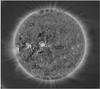 |
Fig. 1 Full Sun intensity map from EUVI on STEREO B on 2008/03/25 at 00:09 UT in the Fe ix,x 171 Å line, including NOAA AR 10987 close to the central meridian in the equator. |
In the present case, we selected, from the daily synoptic time series, two EUVI data sets consisting of 8-h long sequences of 171 Å images taken at 2.5 min cadence. We are restricted to 171 Å images in this study because it is the only EUVI wavelength with the required cadence in the synoptic program. We are also using only a single EUVI viewpoint because the validation of the technique is one of the aims of this paper. A single viewpoint and single wavelength are both adequate for this purpose and allow for a focused paper. Besides, the use of both viewpoints to recover 3D information is not always straightforward. It requires that the same loops are visible, and measureable, in both views. This condition becomes more difficult to meet after the STEREO spacecraft separation exceeds about 15°. Because EUV emission is optically thin, overlapping structures and line-of-sight integration effects make it exceedingly difficult to reliably identify the same loop in both EUVIs. Nevertheless, we have tried to obtain some 3D information for our studied loops using both EUVIs with mixed success. The details are described in Sect. 3.4. Such practical difficulties make it important to have a reliable technique for speed measurements from a single viewpoint.
Our next step is to apply our technique to both three-dimensions (using EUVI observations from both STEREO spacecraft) and to SDO/AIA observations (using 2 or more wavelengths from a single viewpoint).
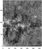 |
Fig. 2 Fe ix,x sub-field intensity map from STEREO B on 2007/08/23 at 00:06 UT showing the anemone-like region and surroundings on the quiet Sun, and the magnetic field lines obtained from potential-field extrapolation. |
The EUVI data were processed to level-1, using the standard routines available in the SECCHI SolarSoft tree. The processing consisted of bias correction, de-gridding, exposure-time normalization, and conversion of digital counts to photons. Next, we applied our wavelet processing technique, as adapted to the STEREO/EUVI images from Stenborg et al. (2008) to clean and increase the contrast of the EUVI images. Briefly, the method employs a multi-level decomposition scheme using the splitting algorithm of a wavelet packet on non-orthogonal wavelets via the  trous wavelet transform, local noise reduction, and interactive weighted recomposition.
The wavelet-cleaned and enhanced 171 Å images reveal that intensity fluctuations are apparently travelling outward in several regions on the solar disk, as well as above the limb. These disturbances can be best seen in movies produced by the EUVI time sequences when the image cadence program is sufficiently high. From our visual inspection of these movies we find that the time gap between images must be less than 3 min for the phenomena to be clearly and unambiguously discerned. This means that we can study kinematics in any EUVI synoptic sequence from the beginning of the STEREO science operations in January 2007 until late August 2009, and until now for observations in the special event buffer taken for 3−4 h daily.
Tracking and measuring the intensity fluctuations presents a challenge because the fluctuations cannot be discerned in individual images. Their brightness is close to the noise level, and they do not appear as discrete features in a given static frame. However, they are readily discernible in a time-lapse movie (see, e.g., Fig. 12 and movie 1). We have encountered similar problems in the tracking of faint features in the solar wind in coronagraph data. They were resolved with the use of the so-called j-maps (Sheeley et al. 1999). These are stacks (in time) of the intensity along a given position angle for a range of elongation angles (or heliocentric heights). The technique enhances the visibility of faint structures making it possible to track intensity fluctuations as low as ~1% of the background to large distances (Sheeley et al. 2008). Similarly, Shine et al. (1994) suggested a space-time image as the best method to track the Evershed flow in sunspot penumbras. Hence, we decided to adopt the j-map approach and devised a procedure to create a gray-scale space-time map of the intensity fluctuations along a chosen path. The series of steps involved are described in detail in Sect. 2.2 because they are crucial for the purpose of this work.
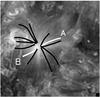 |
Fig. 3 Fe ix,x Intensity map of the anemone-like region and surroundings from STEREO B on 2007/08/23 at 00:06 UT. The black and white lines show the slits defined along particular structures. The corresponding intensities along these slits as a function of time are shown in Fig. 5, where the path denoted as A corresponds to the second map from the top, and B corresponds to the first one. |
2.2. Constructing the Distance-Time maps
The method consists, briefly, of selecting a particular path along a given structure on a given reference image and then watch the evolution through a narrow slit (2 pixels wide) along this path. The procedure is similar to that devised by Sheeley et al. (1999) to track coronal features as they move along a given position angle in the coronagraph field of view. Our method also resembles the one employed previously in the pioneering work of De Moortel et al. (2000, 2002) who posed virtual slits on their target loops in the corona, and then constructed at each slit position running difference images, which thus resulted in corresponding time series from which by wavelet analysis the oscillation characteristics could be inferred.
Hence, we put a virtual “slit”, defining a path that may be curved following the field lines on the EUVI images, with the typical lengths of the slit being about 50 000 km (2007/08/23 case), and 100 000 km (2008/03/25 case). This procedure is illustrated in Figs. 3 and 4, which show the slits as black and white lines. The white lines denote the particular slits used for the present analysis.
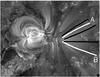 |
Fig. 4 Fe ix,x Intensity map of the NOAA AR 10987 and surroundings from STEREO B on 2008/03/25 at 00:06 UT. The black and white lines show the slits defined along particular structures. The corresponding intensities along these slits as function of time are shown in Fig. 5, where the path denoted as A corresponds to the second map from the bottom, and B corresponds to the last one. |
The fluctuations we want to track tend to occur along EUV features that generally are curved and not necessarily radial. Therefore, we need a slit which has a moderate curvature and can start anywhere in the field of view. To perform the actual measurements, we stack the slit intensity profiles in a rectangular map of distance along the slit versus time. In this representation, features propagating along the slit will appear as inclined intensity ridges. The more discrete the outward moving feature is, the higher its track contrast against the background of the map.
A series of steps is involved to create these Distance-Time maps, which are explained below.
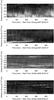 |
Fig. 5 Distance-Time maps: intensity along the slit as function of time. This presentation is apt to reveal propagating features appearing as coherent structures in the hodograms of this map. The maps are obtained with the slits located as depicted in white in Fig. 3 (anemone-like region on 2007/08/23) on the top two panels, and in Fig. 4 (NOAA AR 10987 on 2008/03/25) on the two bottom ones, respectively. |
De-rotation: to be able to position the slit along the same feature in a time series of EUVI images we first have to remove the effects of solar rotation. The wavelet-processed images are grouped in segments of a given time length, and de-rotated to the first frame in the group using standard Solar Soft routines. The routines assume that the corona is rotating rigidly with the photosphere and therefore use a photospheric tracer. However, this assumption is not strictly true and a drift is expected to occur, depending on the latitude of the region under analysis. An easy way to minimize this effect is to make the time length of the segment small enough so that the drift is not noticeable. A time period of 8 hours proved to be reasonable for our purposes.
Path (Slit) definition: once a sequence of images is de-rotated, we manually select a rectangular region of interest (ROI) in the first frame of the sequence. The region must comprise an area big enough to surround the bundle of structures along which we want to track the intensity disturbances. Once such a ROI is identified, one must then define the slits, i.e. pinpoint the paths along the various structures in which the intensity disturbances are intended to be studied. This is done by clicking with the mouse along a given structure at several locations. The points are joined by a spline to define the path, and hence the slit dimension and its position. Figures 3 and 4 show the chosen ROIs and the paths along which the intensity fluctuations are studied.
Distance-Time maps: the slits are then stacked in time, creating distance-time maps. To exemplify the steadiness of the region defined by the slit, we display as a movie in the online material a typical 8-h sequence with the corresponding slit superposed (Fig. 13, movie 2). Figure 5 shows four typical frames from such movies. Different features can be observed in such maps. For example, there are horizontal bright stripes which are often related to lasting bright points, which are not of interest here. We focus on the dimmer, slightly inclined ridges of varying brightness forming a comb pattern, which we interpret as signatures of moving features. The uniformity of this pattern and its common occurrence in randomly chosen and positioned slits in the original images (Figs. 3 and 4) suggest a coronal phenomenon that exists permanently everywhere. These lasting characteristics speak against an interpretation in terms of intermittent sporadic plasma blobs or ejections, but appear to be natural for ubiquitously propagating compressive waves (see Sect. 3).
Speed determination: at this point, we are ready to measure the speeds implied by the hodogram tracks in the maps. As it is common in such height-time measurements, selection effects enter and experience plays a role, as the user must mark at least two locations along the track to characterize the motion. If only two points are used, the track is fitted with a linear model to obtain the average propagation speed. Such a simple constant-speed model is suggested by most of the available data. However, some of the tracks show noticeable curvatures, which tend to occur close to the origin of the slit (i.e., close to the convergence point of the fan-like structures). This curvature implies a varying plane-of-sky speed (See Sect. 3.1).
Next, we looked at the corresponding EUVI-A observations in an effort to obtain a better estimate of the angle subtended by the selected features (loops) to the line of sight (solar surface) and hence, of the true speed. For the March 25, 2008 event it was impossible to identify the individual loop threads (and even the overall loop bundle) in EUVI-A. They show up with very low contrast against the background, which indicates that the loops are seen face-on from EUVI-A. The high inclination of the loops in EUVI-A data implies that the loops would lie approximately along the EUVI-B sky plane. After a careful inspection of the time series of both S/C, we concluded that in EUVI-B the loop threads studied are inclined practically parallel to the solar surface, and therefore we do not need to apply a speed correction for projection effects. In the August 23, 2007 case, the loop geometry is more favorable and we can locate the loops in both views. Using the standard tie-point method for SECCHI measurements (Solarsoft routine “scc_measure.pro”) we find the loops inclined around 30° to the solar surface as viewed from EUVI-B, resulting in an upward speed correction of around 15%. We take this corrections into account in the subsequent discussion.
Periodicity determination: in order to measure the rate at which the tracks appear in the distance-time maps, we made a time/period analysis of portions of the maps obtained at different heights by means of a wavelet-based method as developed by Torrence & Compo (1998). For this analysis, we created 1D time profiles using the intensity as a function of time at a given projected distance from the origin of the slit. The time intensity profiles were constructed by averaging over a given number of pixels along the slit to increase the signal-to-noise ratio (SNR). A typical time profile is displayed for illustration at the top left panel of Fig. 6. It shows oscillations at relatively high frequencies, modulated by a low-frequency background component.
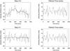 |
Fig. 6 Intensity versus time plots presenting the filtering technique applied to the 1D time series, as obtained from the map corresponding to the slit depicted in white and labeled as A in Fig. 4 (NOAA AR 10987 on 2008/03/25). |
The first run of the wavelet-based periodicity analysis reveals inconclusive results about the periods hidden in the data. The reason for that is a strong low-frequency component, most likely due to the background. We found that the removal of this background trend must be done with care, but that a consistent method to remove the trend up to certain cutoff frequency can be achieved by applying a modified version (1D) of the splitting algorithm of the wavelet-packet analysis technique (see the paper by Stenborg & Cobelli 2003, and the references therein). Once the background trend is found, we can subtract it from the original time series (step 0). The corresponding background-removed time series is shown on the right upper panel of Fig. 6. The same smoothing procedure is applied to the de-trended times series (step 1). The result is shown in the bottom left panel of Fig. 6. The resulting filtered time series already becomes invariant after the first step, as one can conclude by a comparison of the top right with the bottom right panels (see Sect. 3.3).
3. Results of data analysis and discussion
As aforementioned, we analysed the kinematical behaviour and investigated the nature (waves or flows) of the intensity fluctuations observed in different regions of the solar disk during quiet times, i.e., with no activity and far from noticeable dynamic events such as flares or filament ejecta. The regions selected differed in their magnetic field topology, namely, i) located along apparently-open field lines at the edges of active regions and coronal holes (hereafter Configuration I); and ii) located in the quiet Sun (hereafter Configuration II). The analysis was performed on randomly-chosen dates. However, to keep the discussion in focus, we present only the results obtained for two particular dates, namely 25 March 2008 (Configuration I), and 23 August 2007 (Configuration II). The latter has been analysed by Doscheck et al. (2008), using data from Hinode XRT (Golub et al. 2007) and Hinode EIS (Culhane et al. 2007), and therefore a comparison of our results with their Doppler measurements is facilitated. Figure 5 shows a small sample of the maps that we have actually created and analysed.
In the rest of this section, we present the speed distributions of the travelling intensity fluctuations, and discuss different alternatives and their caveats to infer their nature (Sects. 3.1 and 3.2). We then analyse the periodic signature of the pattern observed in the distance-time maps (Sect. 3.3). Finally, in Sect. 3.4 we introduce the relative amplitude of the intensity fluctuations with respect to the background and compare our results to recent works.
3.1. Kinematical considerations
The speeds of the travelling intensity fluctuations can be inferred from the slightly varying inclinations of the ridges in the distance-time diagrams shown in Fig. 5. They are found to be in the 60−90 km s-1 range (see Fig. 7, and Sect. 3.4).
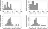 |
Fig. 7 Histograms of the speeds inferred from the four maps shown in Fig. 5, for the 2007/08/23 case (two top frames) and 2008/03/25 case (two bottom frames), with an average value of (63 ± 2) km s-1 (corrected by projection effects) and (86 ± 3) km s-1, respectively. The two corresponding histograms for each case refer to bin sizes of 5 km s-1 (left) and 10 km s-1 (right), respectively. |
Slow-mode magnetoacoustic waves (SMW) in principle can travel in any direction with respect to the mean magnetic field lines. However, its oblique phase speed goes to zero in proportion to the cosine of the propagation angle, and the group velocity (and thus the direction of energy transport) of that wave are constricted to the magnetic field lines. SMWs are also expected to be strongly damped after a few wave periods, because the wave phase speed and the ion thermal speed are close in magnitude. Therefore to detect these waves, it appears appropriate to follow observational features along the field lines, or along the intensity ridges of the coronal emission (see the examples shown in Figs. 3 and 4), which are ordered and oriented by the field through the strong plasma magnetization. In the extreme case of a quickly damped wave, i.e., with a decay time of about 300 s (see, e.g., Ofman & Wang 2002), a prospective wave travelling at 60 km s-1 will cross a distance of at least 60 km s-1 * 300 s = 18 000 km before being damped. Therefore, if the intensity fluctuations actually represent SMW, then we can expect to see wave effects along the individual original slits. Moreover, when individual slits are stacked together to form a distance-time map, a periodic signature should show up. Its visibility is confirmed by the data, in which inclined periodic ridges can be discerned almost up to the edge of the maps.
Even though fluctuations are observed almost along the entire slit, this alone does not help in discerning whether they represent waves or mass flows. Something else is needed to discriminate between the two possibilities, so we tried another method, namely the spatial coherence test. Briefly, if the intensity fluctuations represent waves, they must be in phase, i.e., the intensity pattern observed across field lines should exhibit some spatial coherence. We therefore created distance-time maps by positioning the slits not only along the field lines, but also i) roughly perpendicular to the field lines at different distances from the origin; and ii) with different orientations, from almost parallel to perpendicular to the field lines.
If the slits are positioned perpendicular to the field lines, the following could be expected: i) if the intensity fluctuations are in phase (i.e., all brightenings occurring at once at every field line tracer), bright vertical ridges should appear in the corresponding maps; ii) if a phase shift exists (i.e., a brightening in a following ray appearing slightly later than in a previous ray), these bright ridges should appear inclined; and iii) if no correlation exists between the occurrence of the intensity fluctuations among the different rays, the pattern in the map should be random.
Likewise, if the slits are placed with a given orientation with respect to the field lines, i) vertical ridges should be discerned in the maps if there is a SMW travelling in a direction that matches the direction of the slit (the fluctuation would be in phase for that particular direction); ii) inclined ridges should appear if there is a wave travelling in a slightly different direction than the slit (i.e., a phase shift for the intensity fluctuation travelling on different rays); and iii) a random pattern if none of the above.
3.2. Limitations of the data analysis
Therefore, for a given slit orientation, the pattern observed in the corresponding distance-time maps should tell us whether the fluctuations are in phase. If they are in phase, they are indicative of a large-scale SMW passing by and would favour the “wave” interpretation against the “flow” interpretation. Otherwise, the lack of observed coherence would provide an argument against the “wave” interpretation. The maps we created for the analysis of the two events (not shown here) tend to show some ridge-like features but they are too weak to allow a robust conclusion for either interpretation. This may change when we consider other events in the future.
On the other hand, if the intensity fluctuations represented mass flows, the first question is: could the release of these “mini-blobs” be due to intermittent explosive events with no further energy supply? If so, the trajectory of the mini-blobs should be merely ballistic, i.e., the maximum height reached (in the absence of anything else) would be constrained by the Sun’s gravitational force. The apparent speeds we obtained are much lower than the Sun’s escape velocity (618 km s-1 on the surface, and 609 km s-1 at a height of 10 Mm). So, if no extra energy is supplied after their release, the plasma blobs would not reach to several tens of megameters where we still see fluctuations. Therefore, we do not find evidence for ballistic mass outflows.
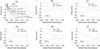 |
Fig. 8 Panel a): normalized global power (NGP) of the existing periodicities in a typical time series as obtained from the wavelet-based analysis (dot-dashed line), and the Lomb-Normalized periodogram (continuous line). Pi indicates the value in minutes of the most significant periods. All labeled peaks have less than 0.01% probability of being due to white noise. Panels b) through f): NGP from the wavelet-based analysis to show how the determination of the background affects the relative intensity of a given period. The number of iterations [n] performed to obtain the different background trends is indicated on each panel along with the value of the dominant period PD. The dashed line in all panels indicates the 95% confidence level for the wavelet-based method. For details see Sect. 3.3. The example shown corresponds to a time series obtained for the slit at the location depicted as A in Fig. 4 at a distance from the slit origin of 36 000 km (on 2008/03/25). |
 |
Fig. 9 25 March 2008 case. Top: typical time series of the relative intensity at a fixed slit position. The approximate window size of the equivalent weighted running average to obtain the background is 22 min (left) and 96 min (right). Bottom colored panels: wavelet power spectrum. The hatched area is below the 95% confidence-level line, and the related data are not reliable. The time-integrated total power (normalized) versus time in minutes is shown to the right of the colored panels. Note that the maximum power peak occurs at a period of ~16 min (left) and ~64 min (right). |
 |
Fig. 10 23 August 2007 case. Top: typical time series of the relative intensity at a fixed slit position. The window size of the equivalent weighted running average to obtain the background is 22 min (left) and 96 min (right). Bottom colored panels: wavelet power spectrum. The hatched area is below the 95% confidence-level line, and the related data are not reliable. The time-integrated total power (normalized) versus time in minutes is shown to the right of the colored panels. Note the peak with maximum power at a period of ~16 min (left) and ~64 min (right). |
Another test for the mass flow interpretation would be indications for distinct plasma blobs in the maps. Notice that if the fluctuations observed represented mass flows, a spreading of the corresponding speed as the mini-blobs evolve with height should be observable, i.e., the ridges in the maps characterizing the individual plasma-blob movement should become wider the farther the blobs are from their origin. At our spatial resolutions, a mini-blob is just an aggregation of plasma composed by many plasma parcels that cannot be resolved. However, as the mini-blob travels along the field line, the individual elements will move at their own speed and hence scatter, resulting in a widening of their speed distribution, which in turn would result in a widening of the corresponding ridge in the map at larger distances from the origin. We see no appreciable widening of the velocity ridges in any of the HT maps we analyzed. So the widening must be at or below one pixel, which corresponds to a velocity spread of ≤1%. This places an upper limit on the speed distribution of the individual parcels. We believe that such a small velocity spread seems unlikely given the complexity and variability of the low atmosphere. Therefore, the lack of velocity spread points against the flow interpretation.
A key test for the wave interpretation is a periodicity analysis of the distance-time maps. The majority of the maps exhibits a salt-and-pepper background pattern, slightly inclined with respect to the vertical, and are marked by the conspicuous presence of intermittent bright emission ridges. The inclination of these features gives the speed of the travelling intensity fluctuations.
3.3. Periodicity analysis
As shown in Sect. 2.2, the background trend must be found and subtracted from the original time series to identify clearly the basic frequencies (periods/wavelengths) underlying the fluctuating time series. Each step of the smoothing algorithm employed to obtain the background can be thought of as simply a recursive low-pass filter (i.e., the time series convolved recursively with a 3-pixels wide boxcar). The higher the number of iterations (hereafter [n]), the smoother the resulting background. For the first iteration, the smoothing procedure is equivalent to a running average with a window size of 3 pixels. Therefore, by exercising this filtering technique with a different [n], the basic frequencies (periods) underlying the fluctuating time series can be revealed.
An example is shown in Fig. 8. Panel (a) shows the normalized global power (NGPTC) obtained with the Torrence & Compo (1998) method (dot-dashed line) for a typical time series built as described in Sect. 2.2. Careful inspection reveals that several peaks are present at particular time periods, as well as possibly unresolved periods that appear as bumps. In order to verify this possibility, we looked for a method to test the hypothesis that a periodic component in the signal is not due to white noise. Therefore, we studied the prospective global periodicities in the time series by means of the Lomb-normalized periodogram (LNP) method (Lomb 1976; Scargle 1982). Unlike Fourier, the LNP is well suited for finite and unevenly sampled data. The continuous line in Fig. 8a, is superposed onto the NGPTC obtained from the wavelet-based method. Note that every significant LNP peak matches the position of a NGPTC peak or bump. The periods corresponding to the most significant LNP peaks, i.e., those peaks that have the lowest probability (less than 0.01%) of arising from random noise, are indicated in the corresponding panel. In panels (b) through (f) of Fig. 8, we plot the NGPTC as a function of period for the background-removed time series. The background is obtained by applying the filtering technique with an increasing [n]. By varying [n], the relative power intensity of the peaks increases toward higher periods in accordance with the increasing degree of smoothing to obtain the background. The periods with maximum power apparently occur in multiples of 8 min. The period of 16 min prevails. Of course, with increasing smoothing one is detecting increasingly longer periods in the fluctuation, as the shorter periods get lost by the smoothing process.
It can be shown using Fourier theory that our recursive smoothing procedure is equivalent to convolving the time series with a suitable kernel of an specific size. In other words, it is equivalent to a weighted temporal smoothing. The size of the kernel depends on [n] (the larger the [n], the wider the kernel). In this way, one can easily assign an equivalent time-window size to the degree of smoothness performed with our recursive procedure to obtain the background, even without knowing the suitable kernel. However, it is worth mention that the shape of the empirically obtained kernel resembles a gaussian for [n] > 2. For a 3-pixel wide boxcar (our case), the equivalence between the number of iterations and the kernel size of the equivalent weighted running average is shown in Table 1 for some [n] values.
Window size in minutes of the equivalent weighted running average to the recursive smoothing procedure for a sample of [n].
Therefore, in the following we refer to an equivalent time-window size when referring to the way the backgrounds were obtained.
Typical examples of the periodicity analysis using the wavelet analysis method developed by Torrence & Compo (1998) are given in Figs. 9 and 10. We show two examples of the weakly compressive fluctuations observed (see Sect. 3.4). In particular, Fig. 9 shows the data for the slit labeled A in Fig. 4 for 25 March 2008. Likewise, data for the slit labeled B in Fig. 3 for 23 August 2007 is displayed in Fig. 10. The top portion of each figure gives the time series of the relative mean intensity at a fixed height range (the range being defined by 5 pixels to increase the SNR). The bottom colored panel shows the corresponding wavelet power spectrum, i.e., the intensity at a given period versus observation time (both in minutes). To the right of the colored panels, the time-integrated total power in arbitrary units versus time in minutes is shown. The fluctuations are defined with respect to the mean value of the time series, which is obtained by our recursive smoothing procedure.
We study the occurrence rate of the ridges observed in the maps, and as a result establish the prevalence of a 16-min period, as well as other periods that seem to be multiples of 8 min (see, e.g., panel (a) in Fig. 8).
Let us now look for a possible solar excitation mechanism. We may conjecture that what we observe are the superposition of the ubiquitous 3-min chromospheric oscillations (with related frequency f1) and 5-min photospheric oscillations (with related frequency f2), which are assumed to leak partly through these layers and somehow pass into the low corona. The frequencies of the two modes are quite close. Wave interference theory shows that the superposition of the two modes will produce a signal with frequency equal to that of the average of the two original signals, modulated in amplitude, the frequency of the modulation being (f1 − f2)/2. Because only the absolute value of the envelope is relevant, the effective frequency, i.e., the so-called beat frequency, will be twice that value (i.e., f1 − f2). Thus, if f1 is 1/3 min-1 and f2 is 1/5 min-1, the resulting period of the beat is about 7.5 min, which is indeed close to the underlying 8 min period.
How to transmit directly the 5-min photospheric oscillations into the corona has been looked into in detail by DePontieu et al. (2005), who showed by numerical simulations that, contrary to the usual believe these waves were evanescent, they can in fact be guided by inclined magnetic flux tubes into the corona. Also, De Moortel et al. (2002) detected 3- and 5-min period oscillations in coronal loops by means of TRACE observations, most likely caused by excitation through an underlying driver inducing loop footpoint motion. Their results suggest that such ubiquitous solar oscillations can indeed penetrate through the transition region into coronal loops.
3.4. Phase speeds and wave amplitudes
Figure 7 shows the distribution of speeds obtained for the two cases considered. Two histograms using different bin size to group the speeds values are shown for each day. Concerning the different speed distributions for the two cases considered, we note that the magnetic topologies (Figs. 2 and 4) are rather different.
Our method allows us to measure the average projected plane-of-the-sky speed, and only if the identification of the same loop in both EUVIs is possible, to infer a true space speed. Generally speaking, however, if the field topologies of the regions differ, one expects to obtain different speed distributions. The angle of orientation of wave propagation with respect to the local magnetic field orientation may range between 0° and 90°. So the actual phase speed may be larger by a factor of 2 or so, e.g. corresponding to an oblique line of sight inclined by 30°. To improve the determination of the phase speed would require exploiting special stereoscopic observations, as was done by Marsh et al. (2009) who could determine the two inclination angles with respect to the local field from the joint STEREO A and B perspectives for a single case. This way they could show that the measured and reconstructed phase speeds may differ by up to a factor of two. In our case, we derived small speed corrections because our measured loops lay close to the sky plane. It is plausible that our technique may preferentially select highly inclined loops since the flows will tend to be more pronounced in such geometries. We do not yet know if this is the case. We plan to study more loop geometries in the future.
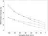 |
Fig. 11 Inferred wave amplitude for the four hodogram panels shown in Fig. 5. The root-mean-square relative line intensity is given versus the equivalent length (in logarithmic units) of the equivalent averaging window in minutes. The squares corresponds to path A, and the asterisks to path B in Fig. 3 for the 23 August 2007 case. The diamonds corresponds to path A, and the crosses to path B in Fig. 4 for the 25 March 2008 case. |
Finally, we present the relative wave amplitude which can be approximated by the variance of the relative emission intensity. The results obtained for the four panels are shown in Fig. 11. The symbols used are explained in the caption. If we take the Full Width at Half Maximum (FWHM) of the equivalent Gaussian (see Sect. 2.2) as the width of our running window, we can easily estimate the size (in pixels, or minutes) of the running window when computing the background with our recursive smoothing procedure. Depending on the size of this averaging time window, the relative amplitude ranges between 2% and 5%, and is smallest at low window lengths, but increases by about a factor of 2 toward larger window sizes. These values are in good agreement with the recent estimates derived for slow magneto-acoustic waves in fan-like coronal loops by Wang et al. (2009), who obtained 3−5% for the density fluctuations with a measured wave velocity amplitude of 1−2 km s-1 from the Dopplershift. Therefore, we claim a detection of comparatively weak-amplitude sound waves.
4. Physical interpretation and conclusion
The evidence exhibited in the present work indicates that propagating fluctuations seem to exist on virtually all open field lines originating from the two regions studied. The studies carried out indicate that these intensity fluctuations do not correspond to discrete blobs of plasma expelled intermittently, but most likely are the signatures of compressible slow-mode magneto-acoustic waves, or may be a mixture of both, whereby the waves appear to dominate the signal and occur continuously. Given on the other hand the spectroscopic evidence of significant and lasting Doppler blue shifts as amply cited above in the Introduction, a scenario appears likely in which the background atmosphere is not at rest but streaming continuously, and the SMWs propagate on this moving coronal plasma. What excites these waves remains to be established. They may be caused by recurrent reconnection, becoming apparent through the footpoint brightenings of the fan-like field lines, as earlier reported by Berghmans & Clette (1999).
The wave generator may be located near the solar surface, where we know that steady magnetoconvection exists, which is believed to act as an engine capable of creating all kinds of waves, with periods that will typically be around the 3 min and 5 min of the basic chromospheric and photospheric oscillations. We do not know why we see multiples of the resulting basic modulation frequency of 8 min, yet we do not want to speculate at this stage of our study on possible mechanisms for the wave excitation. Some relevant discussion on this issue is provided by Wang et al. (2009), but it remains unresolved.
Our study in fact complements recent work of Wang et al. (2009), who found the first clear evidence for propagating low-frequency SMWs in fan-like coronal loops associated with an AR. They had additional information on the fluctuations from Hinode/EIS Doppler shift measurements, which are consistent with their intensity fluctuations but also permitted to estimate the wave velocity amplitude. It typically ranges between 1 km s-1 and 2 km s-1, and the apparent phase speed was found to range from 60 km s-1 to 120 km s-1, which according to the analysis of Marsh et al. (2009) would be consistent with our findings, yet within an unresolved geometrical factor of about up to two. The previous wavelet analysis of Wang et al. (2009) resulted in two prevailing periods, which were about 14 min and 26 min for their intensity fluctuations, values that are close to ours within the measurement uncertainties. So the results of all these three papers are consistent and clearly indicate multiple-period sound waves (in the slow magnetoacoustic mode) propagating everywhere on open magnetic field lines in the lower corona.
In conclusion we can state that the wavelet-processed STEREO/EUVI images clearly reveal intermittent intensity fluctuations travelling outwards along apparently open field lines nearby active region beside coronal holes. Although this phenomenon has been observed before with other instruments, it required data from dedicated observing campaigns. Our method offers many advantages over previous analyses:
-
It enables the study of EUV fluctuations with synopticEUVI observations irrespective of duration,field of view, solar location, spatial resolution or wavelength.
-
It enhances the intensity fluctuations without the use of running difference methods, which invariably introduce a periodic signal in the data.
-
The background trends can be removed in a controlled manner with well-understood effects on the analysis.
-
It is directly applicable to the newly available EUV observations from SDO-AIA opening a new science capability and enhancing the scientific return of the SDO mission.
Hence, the combination of our technique with the synoptic EUV observations should provide a deeper physical understanding of this kind of phenomenon in the future.
Now that the method is validated, we plan to extend it to three dimensions to take full advantage of the STEREO twin-viewpoints observations. We also plan to study the thermal structure of these fluctuations by applying our method to the SDO/AIA observations to take advantage of their multi-wavelength capabilities.
Online material
Movie 1
Access Supplementary Material
Movie 2
Access Supplementary Material
 |
Fig. 12 Movie (movie 1) of running difference wavelet-cleaned and -enhanced images of EUVI-B in 171 A for 2008/03/25. The movie spans 24 h, with an average time gap between images of 2.5 min. To highlight the traveling disturbances, we used as base image for each frame the 5th image prior to the corresponding image. Note the apparently ubiquitous existence of outwardly traveling intensity disturbances. |
 |
Fig. 13 8 h time-lapse sequence (movie 2) showing the slit position along a given pseudo-open field line nearby NOAA AR 10987 on 2008/03/25 (left), and the corresponding height-time map (right). The moving black line indicates the time position on the height-time map corresponding to the frame on the left. |
Acknowledgments
The SECCHI data are produced by an international consortium of the NRL, LMSAL, and NASA GSFC (USA), RAL and U. Bham (UK), MPS (Germany), CSL (Belgium), IOTA and IAS (France).
References
- Berghmans, D., & Clette, F. 1999, Sol. Phys., 186, 207 [NASA ADS] [CrossRef] [Google Scholar]
- Brekke, P. 1993, ApJ 408, 735 [NASA ADS] [CrossRef] [Google Scholar]
- Chifor, C., Young, P. R., Isobe, H., et al. 2008, A&A, 481, L57 [NASA ADS] [CrossRef] [EDP Sciences] [Google Scholar]
- Culhane, J. L., Harra, L. K., James, A. M., et al. 2007, Sol. Phys., 243, 19 [Google Scholar]
- DeForest, C. E., & Gurman, J. B. 1998, ApJ, 501, L217 [NASA ADS] [CrossRef] [Google Scholar]
- Del Zanna, G. 2008, A&A, 481, L49 [NASA ADS] [CrossRef] [EDP Sciences] [Google Scholar]
- DePontieu, B., Erdélyi, R., & De Moortel, I. 2005, ApJ, 624, L61 [NASA ADS] [CrossRef] [Google Scholar]
- De Moortel, I., Ireland, J., & Walsh, R. W. 2000, A&A, 355, L23 [NASA ADS] [Google Scholar]
- De Moortel, I., Ireland, J., Hood, A. W., et al. 2002, A&A, 387, L13 [NASA ADS] [CrossRef] [EDP Sciences] [Google Scholar]
- Doscheck, G. A., Warren, H. P., Mariska, J. T., et al. 2008, ApJ, 686, 1362 [NASA ADS] [CrossRef] [Google Scholar]
- Foukal, P. 1978, ApJ, 223, 1046 [NASA ADS] [CrossRef] [Google Scholar]
- Golub, L., Deluca, E., Austin, G., et al. 2007, Sol. Phys., 243, 63 [NASA ADS] [CrossRef] [Google Scholar]
- Hara, H., Watanabe, T., Harra, L. K., et al. 2008, ApJ, 678, L67 [NASA ADS] [CrossRef] [Google Scholar]
- Hassler, D. M., Dammasch, I. E., Lemaire, P., et al. 1999, Science, 283, 810 [NASA ADS] [CrossRef] [PubMed] [Google Scholar]
- Howard, R. A., Moses, J. D., Vourlidas, A., et al. 2008, Space Sci. Rev., 136, 67 [NASA ADS] [CrossRef] [Google Scholar]
- Isobe, H., Proctor, M. R. E., & Weiss, N. O. 2008, ApJ, 679, L57 [NASA ADS] [CrossRef] [Google Scholar]
- Kosugi, T., Matsuzaki, K., Sakao, T., et al. 2007, Sol. Phys., 243, 3 [NASA ADS] [CrossRef] [Google Scholar]
- Lomb, N. R. 1976, Ap&SS, 39, 447 [NASA ADS] [CrossRef] [Google Scholar]
- Marsch, E., Wiegelmann, T., & Xia, L.-D. 2004, A&A, 428, 629 [NASA ADS] [CrossRef] [EDP Sciences] [Google Scholar]
- Marsch, E., Tian, H., Sun, et al. 2008, ApJ, 684, 1262 [NASA ADS] [CrossRef] [Google Scholar]
- Marsh, M. S., Walsh, R. W., & Plunkett, S. 2009, ApJ, 697, 1674 [NASA ADS] [CrossRef] [Google Scholar]
- McIntosh, S. W., Innes, D. E., De Pontieu, B., et al. 2010, A&A, 510, L2 [NASA ADS] [CrossRef] [EDP Sciences] [Google Scholar]
- Nakariakov, V. N., & Verwichte, E. 2005, Living Rev. Solar Phys., 2 http://www.livingreviews.org/lrsp-2005-3 [Google Scholar]
- Ofmant, L., & Wang, T. 2002, ApJ, 580, L85 [NASA ADS] [CrossRef] [Google Scholar]
- Robbrecht, E., Verwichte, E., Berghmans, D., et al. 2001, A&A, 370, 591 [NASA ADS] [CrossRef] [EDP Sciences] [Google Scholar]
- Sakao, T., Kano, R., Narukage, N., et al. 2007, Science, 318, 1585 [NASA ADS] [CrossRef] [PubMed] [Google Scholar]
- Scargle, J. D. 1982, ApJ, 263, 835 [NASA ADS] [CrossRef] [Google Scholar]
- Schrijver, C. J. 2001, ApJ, 547, 475 [NASA ADS] [CrossRef] [Google Scholar]
- Schrijver, C. J., Title, A. M., Berger, T. E., et al. 1999, Sol. Phys., 187, 261 [NASA ADS] [CrossRef] [Google Scholar]
- Sheeley Jr., N. R., Walters, J. H., Wang, Y.-M., et al. 1999, J. Geophys. Res., 104, 24739 [Google Scholar]
- Sheeley Jr., N. R., Herbst, A. D., Palatchi, C. A., et al. 2008, ApJ, 675, 853 [NASA ADS] [CrossRef] [Google Scholar]
- Shine, R. A., Title, A. M., Tarbell, T. D., et al. 1994, ApJ, 430, 413 [NASA ADS] [CrossRef] [Google Scholar]
- Stenborg, G., & Cobelli, P. J. 2003, A&A, 398, 1185 [NASA ADS] [CrossRef] [EDP Sciences] [Google Scholar]
- Stenborg, G., Vourlidas, A., & Howard, R. A. 2008, ApJ, 674, 1201 [NASA ADS] [CrossRef] [Google Scholar]
- Teriaca, L., Banerjee, D., & Doyle, J. G. 1999, A&A, 349, 636 [NASA ADS] [Google Scholar]
- Torrence, C., & Compo, G. P. 1998, Bull. Meteor. Soc., 79, 61 [CrossRef] [Google Scholar]
- Tu, C.-Y., Zhou, C., Marsch, E., et al. 2005, Science, 308, 519 [NASA ADS] [CrossRef] [PubMed] [Google Scholar]
- Wang, T. J., Ofman, L., Davila, J. M., et al. 2009, A&A, 503, L25 [NASA ADS] [CrossRef] [EDP Sciences] [Google Scholar]
- Wiegelmann, T., Xia, L. D., & Marsch, E. 2005, A&A, 432, L1 [NASA ADS] [CrossRef] [EDP Sciences] [Google Scholar]
- Wilhelm, K., Dammasch, I. E., Marsch, E., et al. 2000, A&A, 353, 749 [NASA ADS] [Google Scholar]
- Wilhelm, K., Dviwedi, B. N., Marsch, E., et al. 2004, Space Sci. Rev., 111, 415 [NASA ADS] [CrossRef] [Google Scholar]
- Wilhelm, K., Marsch, E., Dviwedi, B. N., et al. 2007, Space Sci. Rev., 133, 103 [NASA ADS] [CrossRef] [Google Scholar]
- Winebarger, A. R., DeLuca, E. E., & Golub, L. 2001, ApJ, 553, L81 [NASA ADS] [CrossRef] [Google Scholar]
- Winebarger, A. R., Warren, H., van Ballegooijen, A., et al. 2002, ApJ, 567, L89 [NASA ADS] [CrossRef] [Google Scholar]
- Wuelser, J.-P., Lemen, J. R., Tarbell, T. D., et al. 2004, SPIE, 5171, 111 [NASA ADS] [Google Scholar]
- Xia, L. D., Marsch, E., & Curdt, W. 2003, A&A, 399, L5 [Google Scholar]
All Tables
Window size in minutes of the equivalent weighted running average to the recursive smoothing procedure for a sample of [n].
All Figures
|
Fig. 1 Full Sun intensity map from EUVI on STEREO B on 2008/03/25 at 00:09 UT in the Fe ix,x 171 Å line, including NOAA AR 10987 close to the central meridian in the equator. |
| In the text | |
|
Fig. 2 Fe ix,x sub-field intensity map from STEREO B on 2007/08/23 at 00:06 UT showing the anemone-like region and surroundings on the quiet Sun, and the magnetic field lines obtained from potential-field extrapolation. |
| In the text | |
|
Fig. 3 Fe ix,x Intensity map of the anemone-like region and surroundings from STEREO B on 2007/08/23 at 00:06 UT. The black and white lines show the slits defined along particular structures. The corresponding intensities along these slits as a function of time are shown in Fig. 5, where the path denoted as A corresponds to the second map from the top, and B corresponds to the first one. |
| In the text | |
|
Fig. 4 Fe ix,x Intensity map of the NOAA AR 10987 and surroundings from STEREO B on 2008/03/25 at 00:06 UT. The black and white lines show the slits defined along particular structures. The corresponding intensities along these slits as function of time are shown in Fig. 5, where the path denoted as A corresponds to the second map from the bottom, and B corresponds to the last one. |
| In the text | |
|
Fig. 5 Distance-Time maps: intensity along the slit as function of time. This presentation is apt to reveal propagating features appearing as coherent structures in the hodograms of this map. The maps are obtained with the slits located as depicted in white in Fig. 3 (anemone-like region on 2007/08/23) on the top two panels, and in Fig. 4 (NOAA AR 10987 on 2008/03/25) on the two bottom ones, respectively. |
| In the text | |
|
Fig. 6 Intensity versus time plots presenting the filtering technique applied to the 1D time series, as obtained from the map corresponding to the slit depicted in white and labeled as A in Fig. 4 (NOAA AR 10987 on 2008/03/25). |
| In the text | |
|
Fig. 7 Histograms of the speeds inferred from the four maps shown in Fig. 5, for the 2007/08/23 case (two top frames) and 2008/03/25 case (two bottom frames), with an average value of (63 ± 2) km s-1 (corrected by projection effects) and (86 ± 3) km s-1, respectively. The two corresponding histograms for each case refer to bin sizes of 5 km s-1 (left) and 10 km s-1 (right), respectively. |
| In the text | |
|
Fig. 8 Panel a): normalized global power (NGP) of the existing periodicities in a typical time series as obtained from the wavelet-based analysis (dot-dashed line), and the Lomb-Normalized periodogram (continuous line). Pi indicates the value in minutes of the most significant periods. All labeled peaks have less than 0.01% probability of being due to white noise. Panels b) through f): NGP from the wavelet-based analysis to show how the determination of the background affects the relative intensity of a given period. The number of iterations [n] performed to obtain the different background trends is indicated on each panel along with the value of the dominant period PD. The dashed line in all panels indicates the 95% confidence level for the wavelet-based method. For details see Sect. 3.3. The example shown corresponds to a time series obtained for the slit at the location depicted as A in Fig. 4 at a distance from the slit origin of 36 000 km (on 2008/03/25). |
| In the text | |
|
Fig. 9 25 March 2008 case. Top: typical time series of the relative intensity at a fixed slit position. The approximate window size of the equivalent weighted running average to obtain the background is 22 min (left) and 96 min (right). Bottom colored panels: wavelet power spectrum. The hatched area is below the 95% confidence-level line, and the related data are not reliable. The time-integrated total power (normalized) versus time in minutes is shown to the right of the colored panels. Note that the maximum power peak occurs at a period of ~16 min (left) and ~64 min (right). |
| In the text | |
|
Fig. 10 23 August 2007 case. Top: typical time series of the relative intensity at a fixed slit position. The window size of the equivalent weighted running average to obtain the background is 22 min (left) and 96 min (right). Bottom colored panels: wavelet power spectrum. The hatched area is below the 95% confidence-level line, and the related data are not reliable. The time-integrated total power (normalized) versus time in minutes is shown to the right of the colored panels. Note the peak with maximum power at a period of ~16 min (left) and ~64 min (right). |
| In the text | |
|
Fig. 11 Inferred wave amplitude for the four hodogram panels shown in Fig. 5. The root-mean-square relative line intensity is given versus the equivalent length (in logarithmic units) of the equivalent averaging window in minutes. The squares corresponds to path A, and the asterisks to path B in Fig. 3 for the 23 August 2007 case. The diamonds corresponds to path A, and the crosses to path B in Fig. 4 for the 25 March 2008 case. |
| In the text | |
|
Fig. 12 Movie (movie 1) of running difference wavelet-cleaned and -enhanced images of EUVI-B in 171 A for 2008/03/25. The movie spans 24 h, with an average time gap between images of 2.5 min. To highlight the traveling disturbances, we used as base image for each frame the 5th image prior to the corresponding image. Note the apparently ubiquitous existence of outwardly traveling intensity disturbances. |
| In the text | |
|
Fig. 13 8 h time-lapse sequence (movie 2) showing the slit position along a given pseudo-open field line nearby NOAA AR 10987 on 2008/03/25 (left), and the corresponding height-time map (right). The moving black line indicates the time position on the height-time map corresponding to the frame on the left. |
| In the text | |
Current usage metrics show cumulative count of Article Views (full-text article views including HTML views, PDF and ePub downloads, according to the available data) and Abstracts Views on Vision4Press platform.
Data correspond to usage on the plateform after 2015. The current usage metrics is available 48-96 hours after online publication and is updated daily on week days.
Initial download of the metrics may take a while.