| Issue |
A&A
Volume 526, February 2011
|
|
|---|---|---|
| Article Number | A59 | |
| Number of page(s) | 39 | |
| Section | Interstellar and circumstellar matter | |
| DOI | https://doi.org/10.1051/0004-6361/200912874 | |
| Published online | 21 December 2010 | |
A study of three southern high-mass star-forming regions⋆
1
ETH Zürich, Wolfgang-Pauli-Strasse 27, 8093 Zürich, Switzerland
e-mail: This email address is being protected from spambots. You need JavaScript enabled to view it.
2
Max-Planck-Institut für Radioastronomie, Auf dem Hügel 69, 53121 Bonn, Germany
3
ESO, Karl-Scharzschild-Strasse 2, 85748 Garching-bei-München, Germany
4
I. Physikalisches Institut, Universität zu Köln, Zülpicher Str. 77, 50937 Köln, Germany
5
National Radio Astronomy Observatory, PO Box O, 1003 Lopezville Road, Socorro, NM 87801-0387, USA
Received: 13 July 2009
Accepted: 14 September 2010
Abstract
Context. Based on color-selected IRAS point sources, we have started to conduct a survey of 47 high-mass star-forming regions in the southern hemisphere in 870 μm dust continuum and molecular line emission in several frequency ranges between 290 GHz and 806 GHz. This paper describes the pilot study of the three sources IRAS 12326−6245, IRAS 16060−5146, and IRAS 16065−5158.
Aims. To characterize the physical and chemical properties of southern massive star-forming regions, three high-luminosity southern hemisphere hot cores are observed in continuum and molecular line emission. Based on the results obtained in the three sources, which served as templates for the survey, the most promising (and feasible) frequency setups for the remaining 44 sources were decided upon.
Methods. The sources were observed with the Atacama Pathfinder EXperiment (APEX) in five frequency setups aimed at groups of lines from the following molecules: CH3OH , H2CO , and CH3CN . Using the LTE approximation, temperatures, source sizes, and column densities were determined through modeling of synthetic spectra with the XCLASS program. Dust continuum observations were done with the Large APEX BOlometer CAmera (LABOCA) at 870 μm and the 3 mm continuum was imaged with the Australia Telescope Compact Array (ATCA).
Results. Based on the detection of high-excitation CH3CNlines and lines from complex organic species, the three sources are classified as line rich, hot core type sources. For all three, the modeling indicates that the line emission emerges from a combination of an extended, cooler envelope, and a hot compact component. All three sources show an overabundance of oxygen-bearing species compared to nitrogen-bearing species. While the chemistry in the three sources indicates that they are already in an evolved stage, the non-detection of infrared heating sources at the dust continuum peak of IRAS 16065−5158 points to this source still being deeply embedded. Because this work served as a pilot study, the approach to observe the remaining 44 massive star-forming regions was chosen based on its results.
Conclusions. The three sources are massive, luminous hot cores. While IRAS 16065−5158 seems to be a very young deeply embedded object, IRAS 12326−6245 and IRAS 16060−5146 seem more evolved and have already developed UCHiiregions.
Key words: stars: formation / ISM: lines and bands / submillimeter: general
© ESO, 2010
1. Introduction
Massive stars (M > 8 M⊙) are important building blocks of galaxies. Although they are rare, they provide most of the stellar luminosity and heavily influence their surroundings through energetic interactions throughout their short lifetime. A further understanding of the role of massive stars involves understanding their formation processes, which has always posed a challenge, because the earliest stages of massive star formation are deeply embedded in these objects’ natal dust clouds.
One approach to study high-mass star-forming regions in depth would be to observe a large number of sources in a wide frequency range, which is not yet feasible. Observing the sources in a number of frequency setups to cover many molecular lines is needed to study the prevailing excitation conditions of the molecular gas. In the past, individual sources have either been studied in several frequency setups (see Cesaroni et al. 1994; MacDonald et al. 1996; Olmi et al. 2003; Beuther et al. 2006, to name a few), or surveys of several sources have been performed, mostly on the northern hemisphere, with only very limited frequency coverage (Churchwell et al. 1992; Molinari et al. 2002; Mueller et al. 2002; Sridharan et al. 2002; Shirley et al. 2003). On the southern hemisphere, Purcell et al. (2006) and Urquhart et al. (2007b) have performed line surveys in the mm regime. While many samples of high-mass star-forming regions have been observed in the dust continuum on the northern and southern hemispheres, such as the samples of Beuther et al. (2002); Faúndez et al. (2004); Hill et al. (2005) and Beltrán et al. (2006), no project has so far observed the same sample both in a high-frequency line survey and in dust continuum.
To address the lack of statistically significant sub-mm surveys of southern hemisphere sources in both lines and continuum, we have conducted a survey of 47 high-mass star-forming regions in the southern hemisphere in 870 μm dust continuum and molecular line emission in several frequency ranges between 290 GHz and 806 GHz, based on color-selected IRAS point source criteria. Our selection criteria follow those described in Sridharan et al. (2002), with the exception that our sample includes sources with and without detected radio continuum emission in medium resolution single dish 5 GHz surveys.
This large sample contains sources at very different stages of evolution and will allow a consistent and comparative analysis of these regions.
Out of this survey, we will present in this paper observations of three high-luminosity southern hemisphere hot cores with the Atacama Pathfinder Experiment1 telescope, which served as targets for a template study for our large survey. IRAS 12326−6245, IRAS 16060−5146, and IRAS 16065−5158 (Table 1, from now on we omit the IRAS in the name for brevity) were chosen to be analyzed in this pilot study, because they are the most luminous and line-rich sources in the sample of our study based on their HCO + and SO2spectra, and therefore the most suitable targets to test the feasibility of the project. A fourth very strong hot molecular core of the sample, IRAS 17233−3606, has been analyzed and the results have been published separately (Leurini et al. 2008). Based on the results obtained in these three sources, the most promising (and feasible) frequency setups for the remaining 44 sources were selected.
1.1. Source details
The three sources had already been observed in the course of several maser studies (Walsh et al. 1997, 1998; Caswell 1998, 2001; MacLeod et al. 1998), as well as in the mm continuum survey of Faúndez et al. (2004), the CSsurvey of Bronfman et al. (1996) and the HNCOsurvey of Zinchenko et al. (2000).
We derived the kinematic distances to the sources from the center velocities of the C17O (3−2) line by using the Galactic velocity field description of Kalberla et al. (2007). In the following paragraph, the characteristics of the sources are summarized.
IRAS 12326−6245
The kinematic distance estimated for 12326−6245 from its systemic velocity of −39.3 km s-1 is 4.4 kpc. 12326−6245 features class II CH3OHmasers at 6.7 GHz, OH masers at 1.6 GHz (Caswell 1998) and H2Omasers (MacLeod et al. 1998). Observed at 1.2 mm, 12326–6245 shows compact dust continuum emission (Henning et al. 2000; Faúndez et al. 2004; Hill et al. 2005; Miettinen et al. 2006), which coincides with the location of two peaks of cm continuum emission (Walsh et al. 1998; Urquhart et al. 2007a) observed at high resolution. These peaks correspond to the location of two strong MIR peaks at the Q (20 μm) and N (10 μm) bands (Henning et al. 2000). Molecular line observations in the CH3CN (5−4)2, CH3CN (6−5), CH3CN (8−7) and CH3CN (12−11) series reveal a two-component temperature structure hinting at a hot core embedded in a cooler envelope (Araya et al. 2005). Maps of molecular line data show that 12326−6245 seems to have one of the largest bipolar outflows detected in the southern hemisphere (Henning et al. 2000; Wu et al. 2004). Miettinen et al. (2006) derive a rotation temperature of 34 K from observations of CH3CCHbands.
IRAS 16060−5146
The source has class II CH3OHmasers at 6.7 GHz and OH masers at 1665 MHz, 1667 MHz (Caswell 1998) and 6035 MHz (Caswell 2001). It shows strong, spherical 1.2 mm dust continuum emission (Faúndez et al. 2004; Hill et al. 2005; Miettinen et al. 2006) that peaks at the location of the maser sources. High-resolution radio continuum observations at 3.6 and 6 cm (Urquhart et al. 2007a) show two UCHii regions at the location of the mm peak. We derived 5.5 kpc and 9.4 kpc for the near and far distances, respectively, from the systemic velocity of 16060−5146 (−90.95 km s-1) found in our data. The kinematic distance estimates for this source found in the literature differ somewhat between 5.3−6.1 kpc for the near distance and 9.6 kpc for the far distance, which can be explained with the spread found in the systemic velocities assumed for this source, which range from −88 km s-1 to −91 km s-1.
IRAS 16065−5158
In 16065−5158, OHmaser emission at 1665 MHz, 1667 MHz, and 1612 MHz and a CH3OH6.7 GHz maser has been observed (Caswell 1998). 16065-5158 shows extended 1.2 mm continuum emission (Faúndez et al. 2004) and a UCHii region (Urquhart et al. 2007a). We derive a kinematic distance of 4 kpc and 10.8 kpc for the near and far values of 16065-5158, using a systemic velocity of −62.17 km s-1.
Peak coordinates of the 1.2 mm dust continuum data, distances and IRAS luminosities of the three hot core sources (see text).
2. Observations and data reduction
2.1. Atacama Pathfinder Experiment
2.1.1. Line data
The sub-mm data were taken between November 2005 and November 2006 with the Atacama Pathfinder Experiment Güsten et al. (APEX, 2006) telescope on Chajnantor in Chile.
We used both the APEX 2a heterodyne receiver (Risacher et al. 2006) and the dual frequency 460/810 GHz First Light APEX Submillimeter Heterodyne (FLASH) receiver (Heyminck et al. 2006) for our observations (see Table 2 for details on the receiver setups). As backend, the MPIfR-built Fast Fourier Transform Spectrometer (FFTS) (Klein et al. 2006) was used, which consists of two units with 1 GHz bandwidth each. The pointing accuracy was checked on G327.3−0.6 (Wyrowski et al. 2006), and was found to be accurate within 2″. Most of the data were observed as single pointings. When mapping was done, raster maps with a map size of 40″ × 40″ and beam spacing were observed. The observations were done in the position-switch mode. The off-positions were chosen with an offset of (600″, 0″) in azimuth and elevation from the pointing position and were checked to be free of COemission. All observations were obtained in double sideband mode. Calibration errors were estimated to be on the order of 30%. These errors are influenced by pointing and atmospheric fluctuations, but the largest part of the uncertainty stems from uncertain knowledge of the sideband gain ratios. The data were reduced with the CLASS software package3.
Frequency setup for the molecular line observations.
Table 2 lists the frequencies of the bands of the molecular lines observed with APEX that are subject of the pilot study. These lines were the targets of the frequency setups, but because up to 1.8 GHz bandwidth could be used, lines from many other molecules could be observed simultaneously.
To analyze the chemical composition and physical properties of the three sources, five major setups were used, CH3OH (6−5) at 291 GHz (together with H2CO (4−3) for 16060−5146 and 16065−5158), CH3OH (7−6) at 338 GHz, CH3CN (16−15) at 294 GHz, H2CO (4−3) at 291 GHz and H2CO (6−5) at 436 GHz. The positions of the hot cores were first defined as the peak positions of HCO + (4−3) maps at 357 GHz and later refined by APEX continuum scans.
On-source integration times for APEX2a were around 5−8 min per single pointing setup, and 12−20 min per pointing for FLASH observations, depending on the weather conditions.
2.1.2. Continuum data
In summer 2007, we obtained continuum data for our sources from the Large Apex BOlometer Camera (LABOCA).
LABOCA is a 295 channel bolometer at 870 μm with a field of view of 11.4′ and a beam FWHM of 18.6″ (Siringo et al. 2009). The pixel separation is 36″. To produce a fully sampled map, the data were observed in the raster-spiral mode, with 35 s integration time on source, a spacing of 27″ and 4 subscans. This sets the scanning velocity to about 4′/s and the total integration time on source was on average 2.3 min. 12326−6245 was observed in two scans.
The atmospheric opacity was determined every hour through skydips. The zenith opacity was 0.3 for 12326−6245 and 0.09 for 16060−5146 and 16065−5158. The rms noise for 12326−6245 is 100 mJy/beam, while the rms noise for 16060−5146 and 16065−5158 is 50 mJy/beam.
IRAS 16293−2422, IRAS 13134−6242 and η Carinae were used as flux calibrators and the pointing was checked on η Carinae for 12326−6245 and on IRAS 16293−2422 for 16060−5146 and 16065−5158. The pointing was good within 3″.
The data were reduced with the BoA software package (Schuller et al., in prep.).
2.2. ATCA
 |
Fig. 1 Maps of the HCO + (4−3) line for 12326−6245 (top), 16060−5146 (center) and 16065−5158 (bottom). The (0,0) positions correspond to the 1.2 mm peak positions of Faúndez (2004) listed in Table 1. At each offset position, the velocity and Tmb temperature scales go from −100−20 km s-1 and −5−25 K, −150−0 km s-1 and −5−20 K and −120−0 km s-1 and −5−20 K respectively for 12326−6245, 16060−5146 and 16065−5158. |
High spatial resolution data at 3 mm were taken in October 2006 with the Australia Telescope Compact Array (ATCA) interferometer at Narrabri, Australia. The array was in the H75 configuration with a synthesized beam of 6″ × 4″ for 16060−5146, 5″ × 5″ for 16065−5158 and 6″ × 6″ for 12326−6245 and in the FULL 16256−128 correlator configuration.
The continuum was observed at 87.89 GHz with a bandwidth of 128 MHz and a resolution of 8.8 MHz.
The sources were observed during two nights, PKS 1253–055 was used as bandpass calibrator, Mars was observed on the second night as flux calibrator, the gain calibration for 12326−6245 was done on PKS 1147−6753, and on PKS 1613–586 for 16060−5146 and 16065−5158. The theoretical continuum rms noise level was 3 mJy/beam for the continuum and 130 mJy/beam for the line observations, respectively. The data were reduced with MIRIAD4 and the dirty images were de-convolved with the CLEAN algorithm (Högbom 1974).
3. Observational results
3.1. Line data
Because in the beginning LABOCA data were not available, the three sources were mapped in HCO + (4−3) at 357 GHz to verify the peak position observed in the 1.2 mm continuum maps of Faúndez et al. (2004). First, the regions were mapped with beam spacing to locate the peaks, then the coverage was refined with fully sampled maps around the peak positions (see Fig. 1). The peak positions in 12326−6245 and 16060−5146 are significantly offset from the 1.2 mm continuum peak positions as determined by Faúndez et al. (2004). This is mostly likely owing to a pointing problem in the 1.2 mm continuum data, because in 12326−6245 and 16060−5146, respectively, the peak positions derived by Faúndez et al. (2004) are offset by 6 and 15″ from the LABOCA and ATCA peak positions, which agree well for all three sources. The final pointing positions of the line observations can be seen in Table 3. The offset relative to the ATCA positions is less than a FWHM in all cases. When comparing results of different frequency setups later on, note that the offsets between the different positions are less than 1 / 3 of the FWHM in all but one cases. The extent of the sources in HCO+ (4−3) is larger than the beam, which justifies the determination of beam-averaged column density later on.
Coordinates of the line observations of the three sources.
In order to determine the total column density and the properties of the envelopes, the sources were also mapped in CO(3−2) (Fig. 2) and observed in CO(4−3), CO(7−6) and C17O (3−2) on the peak positions (see Fig. 3). Both the COlines and the HCO+ (4−3) line show clear signs of outflow activity in the wings of all sources and self-absorption at the velocity of C17O . All three sources have very high-velocity outflows with a width of the blue wing, Δvblue, of 30 km s-1 and a red wing width, Δvred, of 20 km s-1 in both 16060−5146 and 16065−5158. In 12326−6245, which was already described as one of the most massive and energetic outflows by Henning et al. (2000), we found Δvblue = 50 km s-1 and Δvred = 60 km s-1. 16060−5146 and 16065−5158 show an asymmetric line profile with a stronger blue shoulder at the peak position of the HCO+ (4−3) emission, which is a sign of motion in the core. At the resolution of the current study, it is not possible to distinguish between infall and rotation as possible origin of the large scale motions. Note that in both 12326−6245 and 16065−5158, the high-J CO the intensity in the outflow wings is stronger than in the lower-J lines and one sees stronger self-absorption. In 16060−5146, however, the outflow wings are less strong in the CO(7−6) line, indication of a lower CO abundance in the high-velocity gas.
 |
Fig. 2 Maps of the CO(3−2) line for 12326−6245 (top), 16060−5146 (middle) and 16065−5158 (bottom). The (0,0) positions correspond to the 1.2 mm peak positions of Faúndez (2004) listed in Table 1. The velocity and Tmb temperature scales go from −100−20 km s-1 and −5−60 K, −150−0 km s-1 and −5−50 K and −120−0 km s-1 and −5−60 K respectively for 12326−6245, 16060−5146 and 16065−5158. |
 |
Fig. 3 C17O(3−2), CO(3−2), CO(4−3) and CO(7−6) transitions. While C17O (3−2) is observed on the peak positions in 16065−5158 (top), 16060−5146 (middle) and 12326−6245 (bottom), the spectra of the remaining transitions were produced by averaging all the spectra taken at the map positions. The dashed line marks the zero level. |
 |
Fig. 4 CH3CN(16−15) data at 294 GHz. We show in blue the synthetic model spectrum (see Tables 29, 30). Note that the spectra for the three sources have been observed with different frequency setups, therefore the SO2 line from the image sidebands appears at different frequencies. The rest frequencies of the |
 |
Fig. 5 LABOCA 870 μm emission (shown as contours), starting from 5σ and continuing in multiples of 1.4σ (see Table 14). The yellow crosses mark the sub-cores in 16060−5146 and 16065−5158. The LABOCA beam is shown as green circle in the lower left of the image. The three-color image shows 3.6 (blue), 4.5 (green) and 8 μm (red) emission from the Spitzer GLIMPSE survey. |
The three sources were observed in CH3OH (6−5), CH3OH (7−6), CH3CN (16−15), H2CO (4−3), and H2CO (6−5). As will be further discussed in the next section, all three sources exhibit a rich spectrum of molecular lines. In 12326−6245 and 16065−5158, we found 18 different species, while in 16060−5146, we found 16 species. As is typical for hot core sources, high-excitation lines up to energies of 346 K above the ground state and lines from vibrationally excited states were observed. Especially the setup around 338 GHz is very rich in lines, with detections of up to 40 lines per GHz. The lines were identified with the programme XCLASS (Schilke et al. 1999; Comito et al. 2005) and the rest frequencies provided by the Cologne database for Molecular Spectroscopy (CDMS)5 (Müller et al. 2001, 2005) and JPL molecular spectroscopy database6 (Pickett et al. 1998). Because the line identification went hand in hand with the LTE modeling of the lines, it is described in more detail in Sect. 4.1. To give an example of the chemical complexity of the sources, the identified lines that were included in the XCLASS modeling are listed for the source 16065–5158 in the online material. Note that it was not possible to perform individual Gaussian fits to all the CH3OHand CH3CNlines included in this list, because some of them were heavily blended with lines from other species in all three sources.
For CH3OH , CH3CN , and H2CO , the parameters of the lines (determined from Gaussian fits) can be found in Tables 4 to 12 in the online material. The average line widths of the CH3OHlines in the three sources are 6 km s-1, 10 km s-1 and 7 km s-1 and of the CH3CN (16-15) lines 6 km s-1, 11 km s-1 and 8 km s-1 for 12326−6245, 16060−5146 and 16065−5158 respectively.
16060−5146 has a slightly broader profile than the other two sources. In both CH3CN (16−15) and the high-excitation CH3OH(vt = 1) lines in 16060−5146, one can see a double-peaked profile (Figs. 4 and 13), which might suggest that the larger line widths seen in this source in the other species are caused by the superposition of two velocity components.
In 16065−5158, a similar double-peaked profile can be found for the highly (torsionally) excited CH3OH(vt = 1) lines. 16065−5158 also displays strong CH3CNlines from the v8 = 1 bending mode, which is not seen toward the other two sources. Looking at the distribution of peak velocities versus energy of the lines, one can see no trend in all three sources and molecules. The peak velocities of 16060−5146 are scattered over a broader field than those of the other two sources.
3.2. Continuum data
3.2.1. LABOCA
While 12326−6245 (see Fig. 5 for the three sources) shows a spherical, centrally peaked morphology at 870 μm, 16060−5146 and 16065−5158 show an extended morphology with one and three peaks, respectively. The latter two sources are also surrounded by secondary peaks, unlike 12326−6245, which is isolated within the LABOCA field of view. Here, the bright MIR cluster seen in the Spitzer Space Telescope Galactic Legacy Infrared Midplane Survey Extraordinaire (GLIMPSE) (Benjamin et al. 2003) emission, on which 12326−6245 is centered is the only sign of activity in the region, while the region immediately around the dust emission traced by LABOCA is dominated by enhanced 8 μm emission, a tracer of photon-dominated regions (PDRs).
In 16060−5146, the dominant feature in the LABOCA field of view is a large bubble that is visible in the MIR emission. The 870 μm emission of 16060−5146 corresponds to an active star-forming site located, at least in projection, at the edge of the bubble. The other cores traced by 870 μm emission can be found tracing the rim of the bubble and in another region to the south of 16060−5146.
16065−5158, which is only 12′ away from 16060−5146, is located in an environment with very active star formation. One finds a very extended region of 8 μm emission, interspersed with infrared dark clouds and an association of bright young stars at the center. 16065−5158 is located right at the center of the association, in a deeply embedded region free of MIR emission. An elongated structure at 4.5 μm (color-coded green) seems to be coming from this deeply embedded region. Because 4.5 μm is associated with hot shocked gas (Cyganowski et al. 2008), this situation is very suggestive of a massive outflow stemming from 16065−5158. The very extended 870 μm emission found in the LABOCA field of view for 16065−5158 traces nearly the whole extent of the active star-forming region visible in the GLIMPSE data.
To obtain source positions, sizes, and peak fluxes, the LABOCA maps (see Fig. 5) were analyzed with the sfind routine in the MIRIAD software package. The integrated fluxes were obtained over the area inside the contour line representing 10% of the peak flux, which corresponds to an average signal-to-noise ratio of 120. The size of the sources was determined fitting a circularly symmetric two dimensional Gaussian source model. The source positions, fluxes, sizes, and the calculated H2column density can be found in Tables 13 and 14. The positions agree within the pointing uncertainties with the 3 mm peak positions derived with ATCA. The column density was obtained from Eq. (1), following Motte et al. (1998); Miettinen et al. (2006)![Mathematical equation: \begin{equation} N({\rm H_2})=1.67\times 10^{-22}\frac{I_\nu^{\rm dust}}{B_\nu({T_{\rm d}} )\mu m_{\rm H}\kappa_{\rm d}R_{\rm d}} ~~[{\rm cm}^{-2}] \label{nh2} \end{equation}](/articles/aa/full_html/2011/02/aa12874-09/aa12874-09-eq58.png) (1)where Iν is the peak flux in Jy/beam, Bν(Td) the Planck function of a blackbody at dust temperature Td , μ is the mean molecular mass assuming 10% contribution of helium, κd the dust absorption coefficient of 0.176 m2/kg linearly approximated at 870 μm from model V (thin ice mantles, n = 106 cm-3, β = 1.8) of Ossenkopf & Henning (1994) and a dust-to-gas mass ratio
(1)where Iν is the peak flux in Jy/beam, Bν(Td) the Planck function of a blackbody at dust temperature Td , μ is the mean molecular mass assuming 10% contribution of helium, κd the dust absorption coefficient of 0.176 m2/kg linearly approximated at 870 μm from model V (thin ice mantles, n = 106 cm-3, β = 1.8) of Ossenkopf & Henning (1994) and a dust-to-gas mass ratio  . Model V is suited for sources in which considerable depletion on ice occurs. Unlike the models with thick ice mantles, which apply for dark clouds, the conditions in model V include the influence of a heating source that is starting to evaporate the ices. Ossenkopf & Henning (1994) give the uncertainties for the dust absorption coefficient to be a factor of 2 for ice covered dust and state that it can be up to a factor of 5 higher in disk regions, where the ice mantles are already evaporated off the grains. As provided by model V, we use β = 1.8 (κ ~ (ν / ν0)β) in this work, which is consistent with values of β = 1.5−2.0 found in massive star-forming regions (Molinari et al. 2000). Using the dust opacities derived by Hildebrand (1983), albeit for grains without ice mantles, as has been done by Beuther et al. (2002), leads to masses and column densities that are about a factor of 4 higher.
We also list the source multiplicity, in this case all the sources above 3σ found within the 11.4′ field of view.
3.2.2. ATCA
Figure 6 shows the mm continuum emission imaged with ATCA. One can see that its distribution agrees well with the peak of the LABOCA 870 μm emission. The ATCA continuum emission is still unresolved in 16060−5146 and 12326−6245. In 16060−5146, two cores can be found in the 3 mm emission, and one of them, core ATCA-a, is associated with the LABOCA peak. The other core, ATCA-b, is too far away from the APEX pointing position to be picked up with the APEX beam of about 19″. Therefore, these two cores cannot be responsible for the double peaked structure seen in the spectra of 16060−5146. Figure 6 also shows the location of the offset positions determined for the molecular line observations. While the somewhat crude determination of the position via the HCO + peaks meant that we may have missed the position of the hot cores by a few seconds of arc, we were still close enough to pick up the hot core emission in the beams.
In Fig. 6, overlaid on the data are the interferometric positions of associated OH(Caswell et al. 1999, 2001, 2004) and CH3OHmasers (Caswell, private communication), as well as the 3 cm and 6 cm peaks of radio continuum emission (Urquhart et al. 2007a). It is remarkable that in 16060−5146, only core A (position 16060−5146 ATCA-a) has associated masers and radio continuum, suggesting that core 16060−5146 ATCA-b might be in a very early evolutionary stage. This core is neither evident in the LABOCA continuum data nor in the Spitzer GLIMPSE MIR data.
The ATCA data provide a precise position of the core (see Table 15). The beam de-convolved source sizes, positions, and fluxes for the sources were determined from the image plane with the imfit task in the MIRIAD software package.
 |
Fig. 6 ATCA 3 mm continuum data (solid lines) top 16060−5146 (contour steps −3, 3, 5, 7...σ, with σ = 0.1 Jy/beam), middle 16065−5158 (contour steps −3, 3, 5, 7...σ, with σ = 8 mJy/beam) and bottom 12326−6245 (contour steps −3, 3, 5, 7...σ, with σ = 0.14 Jy/beam). The synthesized ATCA beam is shown in the lower left corner. LABOCA 870 μm continuum is shown in gray-scales. Symbols: red: radio continuum (Urquhart et al. 2007), blue: OH maser positions, green: offsets of the APEX line observations, turquoise: IRAS position, yellow: CH3OHmaser (Caswell et al. 1998). |
 |
Fig. 7 Zoom-in of the Spitzer GLIMPSE composite image of 3.6, 4.5 and 8 μm emission. LABOCA 870 μm emission is shown as contours, starting from 5σ. The small blue circles and crosses mark the position of the 6 cm and 3.6 cm continuum (Urquhart et al. 2007). 16060–5146: the blue boxes show the location of the ATCA 3 mm continuum emission (marked “a” and “b”). 16065−5158: the cross and circle marking the radio continuum emission are shown in white. |
 |
Fig. 8 Spectrum of 12326−6145. The synthetic model spectrum of CH3OH (7–6) is shown in red. In the upper plot (vt = 1), the synthetic spectrum of the torsionally excited CH3OHtransitions (red) is shown. |
 |
Fig. 9 Spectrum of 12326−6245. The synthetic model spectrum of CH3OH (6–5) is shown in red. In the upper plot (vt = 1), the synthetic spectrum of the torsionally excited CH3OHtransitions (red) is shown. The two lines marked (mirror) in both plots show lines that lie outside the shown frequency range, but were folded into the spectrum owing to imperfect filter edges. |
3.2.3. IR and radio emission
In addition to the 870 μm continuum observed with LABOCA and the 3 mm continuum observed with ATCA (this work), the associated fluxes of point sources found in the Spitzer GLIMPSE survey in the 3.6, 4.5, 5.6 and 8 μm bands observed with the Infrared Array Camera (IRAC) and in the MSX mission at 8.3, 12.1, 14.7 and 21.3 μm (Egan et al. 2003) were obtained. Photometry on the Spitzer MIPSGAL 24 and 70 μm images (Carey et al. 2006) could not be performed, because the sources are saturated in all cases. All the three regions show extended 8 μm emission, which is commonly associated with emission of photon-dominated regions (PDRs) owing to the IR features of polycyclic aromatic hydrocarbons (PAHs).
In order to find the infrared point sources associated with the 870 μm dust peaks, we searched the catalogs within a radius of 9″, the LABOCA beam, around the dust peak. When studying environments of high-mass star formation, one frequently encounters a situation where many infrared sources cluster in one single dish beam – in this case the LABOCA beam – because massive stars are thought to form exclusively in clusters (see Fig. 5). Because many of the young high-mass proto-stellar candidates are very red and bright, they are saturated in the 8 μm band and therefore appear with null values in the GLIMPSE point source catalog (Kumar & Grave 2007), so when a null value at 8 μm was found, we did a manual check on the image to distinguish between sources with no detectable emission at 8 μm and those that are saturated. If the GLIMPSE data was saturated at 8 μm, the MSX value was used.
For 16060−5146 and 12326−6245, both MSX and GLIMPSE emission is associated with the hot core traced by the 3 mm continuum observed with ATCA. In 16065−5158 however, there is neither an MSX nor a GLIMPSE source at the position of the hot core, yet both types of sources can be found a few seconds of arc offset from the hot core, which might indicate an external heating source or a deeply embedded UCHiiregion.
For cm wavelengths, archival 3 cm and 6 cm ATCA data published by Urquhart et al. (2007a) were obtained for the hot cores in 12326−6245 and 16060−5146. In 16065−5158, there is an offset of 4.3″ between the mm position obtained from ATCA and the ATCA cm position (see Fig. 6). The cm emission in this source has a negative spectral index of −0.9, hinting at synchrotron emission. No extragalactic object could be found at this position in the NED database. This could be similar to the situation in W3(H2O), where a synchrotron source (Reid et al. 1995) can be found in a hot core. Note that Urquhart et al. (2007a) state that the spectral indices of individual sources might not be reliable in all cases, because the ATCA is not a scaled array at the observed frequencies (which would provide comparable resolution at the different wavelengths) and the measurements may sample different spatial scales.
Figure 7 shows a zoom-in on the region of the 870 μm peak. In 12326−6245, the IR flux is coming from a bright cluster of objects. One can see emission at 4.5 μm (color-coded green) surrounding the cluster, which is a sign of shocked gas (Cyganowski et al. 2008) and can point to outflow action. In 16060−5146, the peak of the 870 μm emission can be associated with a single object. There is weak 4.5 μm emission at the edge of the IR source. 16065−5158 has no associated IR source at the position of the 870 μm peak. There is however a strong elongated 4.5 μm emission. This situation is suggestive of a deeply embedded young object with a strong outflow.
4. Derivation of physical parameters
4.1. LTE modeling
We observed our sources in lines from CH3CN , CH3OH , and H2CO , which are useful tracers of temperature. While classically rotational diagrams have been used to determine rotational temperature, Trot, and column density, N, of a molecule (see Mangum & Wootten 1993; Olmi et al. 1993), we make use of an LTE approach developed by Schilke et al. (1999) and further improved by Comito et al. (2005). Implemented into the program XCLASS, it allows us to model synthetic spectra that take line blends and optical depth effects into account and furthermore allows us to simulate a double sideband (DSB) spectrum. Input parameters for the simulation are source size, temperature, column density, line widths, and offset from systemic velocity. It is possible to simultaneously model transitions in several frequency bands and include more than one component, i.e. a core and an envelope component and/or several velocity components. If there is a hot core and cold envelope component, both components need to be modeled independently though, i.e. the cold component is not absorbing the hot component, because we do not know the source geometry. Figures 4, 8, and 9 give an example of a synthetic spectrum for a single molecule overplotted on the measured sub-spectra, while Figs. 10−15 in the appendix show the synthetic spectra of all included species.
The degeneracy between column density and source size can be solved for species where both optically thin and thick lines are present, as we did for CH3CNand to some degree CH3OH . For species where only one or two lines were available to model, only the beam-averaged column density was derived, and for species that we assume to reside in the hot core, a rotation temperature Trot = 150 K (Schilke et al. 2006) was assumed while for species located in the more extended envelope 50 K was chosen, unless we had both optically thick and thin lines to derive a temperature from the model.
The lines were identified with the catalogues of the CDMS and the JPL (Pickett et al. 1998; Müller et al. 2001, 2005) as a reference for the rest frequencies.
The tables with the detected lines for the three sources can be found in the online material (Tables 16 to 28) – here we will present the results of the modeling.
XCLASS produces a synthetic spectrum (model) of all species and transitions included in the modeling, which is then overlaid on the data. For CH3CN , we performed a χ2 analysis on the synthetic model spectrum to determine the best-fit model, while for the remaining setups a comparison by eye was done to decide on the best fit. This was necessary to account for the high complexity when modeling several often blended transitions in the double sideband spectra. For sources labeled “b” in Tables 29−31, the lines are weak and/or blended with many other lines, so that the fit is less accurate than a fit marked “c”.
If both temperature and source size were fixed, the column density could be determined to an accuracy of 10%, assuming perfect calibration. The uncertainties introduced when modeling both source size and temperature are discussed in the following sections. This modeling is done under the assumption of LTE, which may not necessarily be valid for every molecule and source, although it is a reasonable choice given the high densities. Nonetheless, this method gives us a good and fast overview on the chemical composition of the sources, and it can be applied to a large sample of sources with considerably less effort than individual non-LTE modeling would require.
The results of the modeling can be found in Tables 29 to 31. Tables 32 to 34 show the model results for those species that were modeled in several frequency setups, namely CH3OH , CH3CN , H2COand SO2 . For some species, marked as f in the Tables, we modeled isotopologues, using ratios of 12C/13C = 60, 32S/34S = 23, 14N/15N = 300 (Wilson & Rood 1994) and 16O/17O = 1500 (Wilson & Rood 1994; Wouterloot et al. 2008).
Properties of the 870 μm continuum as derived from the LABOCA observations.
Positions of the LABOCA 870 μm continuum emission peaks.
ATCA 3 mm continuum parameters.
4.1.1. CH3CN
The symmetric top molecule CH3CNis an appropriate temperature tracer (Araya et al. 2005). The data and the synthetic spectra are displayed in Fig. 4. Owing to the CH3CNlines up to the K = 7 transition in 16065−5158, we used a compact hot component to model the higher excitation lines and additionally a more extended, cooler component to model excess in the K = 0 – K = 2 transitions. Beause this setup also includes some  lines, we had both optically thick and thin transitions to solve the N/θ degeneracy and obtain source sizes. While 16065−5158 and 12326−6245 can both be modeled with a two-component fit displaying one hot, compact component and one extended, cooler one, it is also possible to obtain reasonable results for 12326−6245 with only a hot compact component. The two-component structure is attributed to a hot dense core inside a colder, extended envelope. 16060−5146 had to be modeled with two hot, compact components with a velocity difference of 9 km s-1. This effect, which is not obvious in every species studied here, suggests a complicated velocity structure for parts of the molecular gas in this source.
We obtained physical sizes assuming near distances for 16060−5146 and 16065−5158 of 0.03 pc for the hot component in 16065−5158, 12326−6245 and for the two components in 16060−5146. The extended components in 16065−5158 and 12326−6245 are 0.1 pc each. Tables 32 to 34 show the results for the CH3CNmodeling.
4.1.2. CH3OH
For all three sources, data for the CH3OH (7–6) band were obtained in a setup at 338 GHz, including also the torsionally excited vt = 1 CH3OH lines at 337.6 GHz. The CH3OH (6−5) lines at 290 GHz were observed in all three sources, while for 12326−6245, the torsionally excited lines at 289 GHz were covered in a different frequency setup. Both the J = 6−5 and the J = 7−6 series were modeled with XCLASS under the assumption of LTE.
To obtain the temperature for the hot compact component in the J = 7−6 band, the optically thin torsionally excited lines and the higher excitation lines in the vt = 0 bands were used. In combination with optically thick lines in the band, the N/θ degeneracy could be resolved. The torsionally excited lines at 289 and 337 GHz also contain a line with higher optical depth, from which we could obtain an estimate of the source size for this component.
For details of the model in 12326−6245, see Figs. 8 and 9, while plots of the remaining two sources can be found in the appendix. The synthetic model spectrum in Fig. 8 overestimates the torsionally exited lines, which is because of the added complexity of modeling the torsionally exited vt = 1 lines simultaneously with the hot component of the vt = 0 lines.
In 16060−5146, the line profiles are much broader owing to a blend of two hot compact components and one extended component, and the spectra suffer from a worse baseline than the spectra for the other two sources. We could obtain a good fit for two hot components, but because of the complexity of the data, only a beam-averaged column density could be obtained for the cold component. The results of the CH3OHmodeling can be found in Tables 32−34.
4.1.3. H2CO
Because it is a slightly asymmetric rotor, H2COis a good tracer of kinetic temperatures (Mangum & Wootten 1993) and it is quite ubiquitous in regions of star formation (Mangum et al. 1990; Mangum & Wootten 1993).
In this survey, we observed H2COin all three sources in the H2CO (4−3) transitions at 291 GHz, and in 16065−5158 and 16060−5146 also in H2CO (6−5) lines at 437 GHz. One can obtain a reasonable fit to the two transitions with a hot compact core and a cold extended envelope component. The results of the H2COmodeling can be found in Tables 32−34, while the spectra and synthetic models can be found in Figs. 10, 12, and 14 in the appendix. For 12326−6245, only the H2CO (4−3) transition was observed. In 16060−5146, we could not model the hot H2CO emission with two velocity components, as we did for CH3OHand CH3CN .
4.1.4. S-bearing species
We observed the lines from the S-bearing species CS, H2CS , SO, and SO2in our frequency setups. For the H2CS (10−9) line, only the beam-averaged column density for a fixed temperature of 50 K could be determined, while the other species were observed in several lines.
We observed the isotopologic C33S (9−8), C33S (6−5), and C34S (7−6) transitions in CS, while no C32Sline was included in any of the setups. Assuming isotopic ratios of 32S/34S = 23 and 32S/33S = 127 (Wilson & Rood 1994; Chin et al. 1996), we could model CSand SOconsistently over the frequency bands. The same was not possible for SO2 . Apart from the SO2 (5−4) line at 351.3 GHz, which has a lower level energy of 19 K above ground state, the other SO2lines cover higher excitation conditions, which are between 76 K and 770 K above ground state energy. The results of the SO2modeling can be found in Tables 32−34, while the results for the remaining species are given in Tables 29−31.
4.1.5. Uncertainty estimates
To estimate the errors of the modeled parameters, we performed an χ2 analysis for the CH3CN (16−15) band in 12326−6245 with a fixed source size, varying temperature T, and column densities N. This indicated uncertainties of up to 40% in T and up to 23% in N within the 3σ confidence limit, which we consider as typical for only one frequency setup and no line blends from either sideband. It is evident from Tables 32−34 that in some cases the simultaneous modeling of the hot or cold component of a species could not be done consistently in two different frequency setups. This discrepancy is smaller than a factor of 5 (apart from the cold component of CH3CN (19−18) in 16065−5158) though, and could have several reasons:
First, there can be uncertainties in the flux calibration and pointing, because the data were taken at different times. In addition, in 16060−5158 and 16060−5146 the two setups were observed with a positional offset of 8″ to each other. While at these positions the emission is still covered in the beam, influences of the source geometry might already play a role.
Based on the modeling results of the CH3CN (16−15) band alone, a common line width for the hot and cold component was assumed for the CH3CN (19−18) transitions. This could be another potential cause for discrepancies, but the heavy line blending of the CH3CN (19−18) band does not allow us to derive a reliable line width for the hot component. The line widths from the XCLASS modeling listed in Tables 32 to 34 are intrinsic line widths, and most of the lines are influenced by a high optical depth (see also observed average line widths in the results section), which complicates the determination of the line widths.
Results of the line modeling for 16065−5158 (−62.2 km s-1).
Results of the line modeling for 16060−5146 (−91 km s-1 ).
Results of the line modeling for 12326−6245 (–39.3 km s-1 ).
4.2. Spectral energy distributions
To obtain the dust temperatures and luminosities for the three sources, the spectral energy distribution (SED; i.e., flux density vs. frequency) was analyzed for each source. Estimates of the dust temperatures were obtained by fitting graybody plus free-free spectra to the SEDs (see Fig. 16). For all three sources a power-law dependence of the dust opacity with β = 1.8 was used (see Sect. 3.2.1), based on the dust properties used to derive the masses and column densities of the three sources (Ossenkopf & Henning 1994). We also estimated total luminosities by integrating the fluxes under the SEDs. Note that the GLIMPSE fluxes are not corrected for extinction.
12326−6245 and 16060−5146 were modeled using three different components, while one was used for 16065−5159. The data at 3.6−12 μm trace the hot, compact radiation source that is already well developed in the infrared, while the data points between 24 μm and 3 mm represent the contribution from the colder, more extended dust envelope. The IRAS points at 60 and 100 μm are taken from the high-resolution IRAS Galaxy Atlas (IGA) data. They represent upper limits to the IRAS flux. The cm continuum data, which represent the contribution of free-free emission from an associated UCHiiregion, is modeled as third component. In 16065−5158, only the cold, extended envelope was modeled, because the radio continuum and infrared data are offset from the dust peak.
For 12326−6245, a dust temperature of 77 K was derived with the graybody fit for the extended component. For the hot component traced by the Spitzer IRAC points, the blackbody fit resulted in a temperature of 390 K. The luminosity of the 77 K extended dust component is 1.0 × 10⁵ L⊙ and the one derived from the 390 K compact component 74 L⊙.
16060−5146 has a dust temperature of 63 K, a temperature of the compact component of 500 K and luminosities of 2.4 × 10⁵ L⊙ and 490 L⊙ for the extended and compact components, respectively.
For 16065−5158, the dust temperature was derived to be 50 K, but in this source, it is hard to constrain the parameters, because only the ATCA 3 mm emission and the LABOCA 870 μm emission are associated with it, because IRAS and MSX values give but upper limits. The luminosity of the extended component is 0.6 × 10⁵ L⊙.
The spectral energy distributions show that the 3 mm sources in 12326−6245 and 16060−5146 are dominated by free-free emission and by dust radiation for 16065−5158.
4.3. Spectral types
To obtain the spectral type of the mm-sources, we estimated the Lyman continuum flux from the cm observations of Urquhart et al. (2007a), which trace the free-free emission of the UCHii region.
Because that emission is optically thick from both regions, we obtained their parameters by fitting the spectral energy distribution with the theoretical spectrum of a homogeneous constant density plasma (Garay et al. 2006). For 12326−6245, an emission measure of 2.6 × 10⁹ pc cm-6 and a Lyman continuum flux of 8.2 × 1048 s-1 were obtained, leading to a spectral type between O6.5 and a stellar luminosity of L = 1.5 × 10⁵ L⊙, according to Panagia (1973).
For 16060−5146, the emission measure is 4.0 × 10⁸ pc cm-6, the Lyman continuum flux 1.5 × 1049 s-1 and the spectral type was found to be between O6 and O5.5 with L = 2.5−4.0 × 10⁵ L⊙.
This kind of analysis works with the assumption, that the Lyman continuum luminosity of the source is dominated by the emission of one object.
 |
Fig. 16 Spectral energy distributions for the three sources. The IRAS fluxes (downward pointing triangles) are taken from the high-resolution IRAS Galaxy Atlas (IGA) data. The empty squares and triangles show the MSX and Spitzer GLIMPSE fluxes respectively, the filled circles the ATCA fluxes and the filled triangle and square the bolometer fluxes from SIMBA and LABOCA. |
Properties of 16065−5158 (–62.2 km s-1 ) as derived from LTE modeling of CH3CN , CH3OH , H2COand SO2 .
4.4. Mass estimates
Table 35 lists the dust masses derived from the 870 μm LABOCA observations as well as the virial masses derived from the line velocity dispersion of the C17O(3−2) line. Mvir in M⊙was derived according to MacLaren et al. (1988) and Miettinen et al. (2006)![Mathematical equation: \begin{equation} \label{eq:virmass} M_{\rm vir}=0.5 \Delta v^2 d \Theta_{10} \kappa ~~[\Msun]. \end{equation}](/articles/aa/full_html/2011/02/aa12874-09/aa12874-09-eq134.png) (2)The beam-deconvolved source sizes at the 10% flux contour were taken as the angular source sizes Θ10 in ″. κ ~ 1.3 is a correction factor to correct for the average radial density dependence. We estimated the dust masses in two ways. Mwarm gives a measure of the masses of the warmer component associated with the IRAS source, as traced by the graybody fit of the SED, while Mext traces the masses of the extended cooler envelopes. The dust masses were derived using Eq. (3), following Miettinen et al. (2006), with a dust absorption coefficient, κd, of 0.176 m2/kg (Ossenkopf & Henning 1994) (model V) and a dust-to-gas ratio
(2)The beam-deconvolved source sizes at the 10% flux contour were taken as the angular source sizes Θ10 in ″. κ ~ 1.3 is a correction factor to correct for the average radial density dependence. We estimated the dust masses in two ways. Mwarm gives a measure of the masses of the warmer component associated with the IRAS source, as traced by the graybody fit of the SED, while Mext traces the masses of the extended cooler envelopes. The dust masses were derived using Eq. (3), following Miettinen et al. (2006), with a dust absorption coefficient, κd, of 0.176 m2/kg (Ossenkopf & Henning 1994) (model V) and a dust-to-gas ratio  . Bν(Td) is the Planck function of a blackbody at dust temperature Td , Sν the integrated flux in Jy and d the kinematic distance in kpc.
For the warm component, Tdas derived from the SED and the peak fluxes were used, while the mass of the extended dust emission was derived with the integrated intensity within the 10% contour and assuming a dust temperature of 20 K for 12326−6245 and 30 K for 16065−5158 and 16060−5146, respectively. They were assumed to be equal to the gas kinetic temperatures derived in the CH3CNmodeling, following Miettinen et al. (2006). For 16060−5146, where the CH3CNwas modeled without a cold component, the temperature derived from CH3OH was taken instead. ![Mathematical equation: \begin{equation} M_{\rm gas}=\frac{S_{\nu}d^2}{B_{\nu}(T_{\rm d} ) \kappa_{\rm d} R_{\rm d}} ~~[\Msun] \label{eq:mass} \end{equation}](/articles/aa/full_html/2011/02/aa12874-09/aa12874-09-eq141.png) (3)
(3)
Dust masses derived from LABOCA 870 μm emission.
5. Discussion
5.1. Molecular line data
The considerable band width of the FFT spectrometers at APEX and the huge number of molecular species that we detected in each source enabled us to study their chemical composition. To facilitate a comparison, the molecular emission was divided into two classes, the hot and the cold molecules following the analysis described in Sect. 4.1, with rotational temperatures above 100 K and below 100 K respectively, which corresponds to the ice evaporation temperature for complex organic molecules (Bisschop et al. 2007).
Several molecules, CH3OH , CH3CN , H2CO , and SO2were observed in more than one frequency setup. In these cases it was not always possible to model the species with one consistent set of temperatures and column densities. The reason for this might be either calibration uncertainties between the bands or deviations from local thermal equilibrium.
In Fig. 17 the abundances in the hot and cold component are shown. In 16060−5146, only CH3OHand CH3CNwere modeled with two hot components. In the remaining species, it was impossible to resolve two hot components, even though large line widths often point in this direction. In all three sources, one can see a trend of observing higher abundances in the O-bearing species than in the N-bearing species in the hot component.
Chemical differentiation between N- and O-bearing species has been observed in several high resolution studies of hot molecular cores, among them W3(OH) (Wyrowski et al. 1999) and Orion-KL (Sutton et al. 1995). In the latter, the “hot core” is abundant in complex, saturated N-bearing species, while the “compact ridge” shows high abundances of complex O-bearing molecules. With interferometric observations, Liu (2005) resolve a similar differentiation in the sources E and F in G9.62+0.19, a high-mass star-forming region with similar distance and luminosity to the three sources presented here. Because the chemical differentiation is only resolved with high spatial resolution observations, one would not expect to find the difference in a single dish beam. This leaves the question why one sees a higher abundance of O-bearing species in the three sources of our sample. One possibility is that the complex O-bearing molecules stem from a more extended region and their emission is therefore less beam-diluted.
Rodgers & Charnley (2001) argue that a higher abundance of O-bearing species might suggest an earlier evolutionary stage where the hot core has developed into a rich O-bearing chemistry in the first 104 yr before evolving into a nitrogen rich state, but placing our sources at this young state is inconsistent with the high abundance of CH3CNfound here. The total fraction of N observed is on the order of 3 × 10⁻⁸, 3 × 10⁻⁹ and 5 × 10⁻¹⁰ for 16065−5158, 12326−6245 and 16060−5146. This fraction was made up of CH3CN , HNCO, HC3N , and C2H5CN . Most of the nitrogen in hot cores is however locked up in the N-bearing species N2H + and NH3 , which were not covered by any of our receiver setups.
On the other hand, it is conceivable that the complex N-bearing species, which according to the above-mentioned interferometric studies are expected to be found closest to the hot core, have already been destroyed by the radiation of the young star, placing the sources at a slightly later stage of the hot core phase. For 16060−5146 and 12326−6245, this would be consistent with the discovery of cm continuum emission at the position of the 870 μm peak. Another origin of the high abundance of O-bearing species could be a different composition of the initial grain mantles as discussed by Charnley et al. (1992) and modeled by Caselli et al. (1993) with thermal effects.
In Fig. 17, the beam averaged molecular abundances with respect to H2are compared with those derived for G327.3−0.6 (blue), NGC 6334I (green, Schilke et al. 2006) and 17233−3606 (cyan, Leurini et al. 2008)), which were also obtained with APEX and analyzed in the same way as our data. To compare with a well-studied northern hemisphere hot core, the abundances of G34.3+0.15 (MacDonald et al. 1996) were also included. Overall, one can see good agreement between our data and the other four hot cores for the cold envelope molecules, apart from the slight overabundance of SOand SO2in our sources.
Comparing the hot species, it is obvious that while they are line rich, our sources are weaker in their line emission than the other sources. The deficiency of nitrogen-bearing species in the hot component is pronounced when comparing with the other sources. Beuther et al. (2009) do not detect any N-bearing species toward two young sources in their high-resolution study of hot cores performed with the SMA. They explain the lack of N-bearing species by saying that these need more time to evolve or warmer gas. Because we are detecting lines from gas with T > 200 K, it is not likely that the gas is not warm enough for nitrogen chemistry. The association of 16060−5146 and 12326−6245 with UCHiiregions also rules out the hypothesis that they are still at an early evolutionary stage.
A prominent feature of the three sources is the high abundance of sulfur species. According to Viti et al. (2004), the sulfur species are expected to show a time-dependent signature. In their models, the authors predict the SO/H2CS ratio to be around one at earlier times and then lowering, which is not observed in any of our sources.
Van der Tak et al. (2003) model the sulfur chemistry in the envelopes of young massive stars. The abundances they derive for CSand H2CSagree with those found in our work. SO2and SO, however, are observed here at much higher abundances. The derived SO2abundances compare to those of the SO2“jump” model of the inner envelopes by Van der Tak et al. (2003). Beuther et al. (2009) discuss the use of CS, SOand SO2as chemical clocks, with CSas a suitable tracer for the earlier stages, while SOand SO2better trace the more evolved stages. This picture is consistent with our data.
 |
Fig. 17 Fractional abundances in the three sources for T < 100 K (cold component, top plot) and T > 100 K (hot component, bottom plot). Red triangles show abundances for G34.3+0.15 (Macdonald et al. 1996), green stars for NGC 6334I, blue stars for G327.3-0.6 (both Schilke et al. 2006) and turquoise stars for 17233–3606 (Leurini et al. 2007). The red lines indicate those molecules where the modeling of different transitions resulted in different column densities (see Tables 34 to 33). |
5.2. Continuum data
Modeling of the spectral energy distributions of the three sources revealed that the 3 mm continuum in 16060−5146 and 12326−6245 is dominated by free-free emission, pointing toward a more evolved stage of the sources. This is consistent with the infrared data and the radio continuum data observed by Urquhart et al. (2007a), which also point toward 16065−5158 as the most embedded and least developed object of the three.
The luminosities derived from the ionized regions in 12326−6245 and 16060−5146 differ by about a factor of 2 from the FIR luminosities derived from the IRAS fluxes. As Garay et al. (2006) discuss, these differences might result because part of the stellar luminosity is absorbed by the dust or there might be stars in the region contributing to the FIR luminosity, but which are not hot enough to ionize the gas. The derived luminosity also indicates that the three sources are most likely placed at their near distance, because they would otherwise have to harbor an extremely massive star more luminous than O4.
Comparing the dust mass estimates for the three sources, the virial and continuum masses agree well for the near distance, indicating that the sources are likely bound. To get an estimate of the upper limit for the mass that might be concentrated at the innermost hot component, we determined the mass using the temperature derived from the SED model and the peak flux of the 870 μm continuum. These masses are a factor of about four lower than the envelope masses for 12326−6245 and 16065−5158, while they are about a factor of 2 lower for 16060−5146, indicating that this source is very centrally peaked.
All three sources have been observed by Faúndez et al. (2004), while 12326−6245 and 16060−5146 have also been observed by Miettinen et al. (2006) and Hill et al. (2005). Taking into account the different ways the integrated fluxes used, our masses agree well within factors of about 2 with the estimates by these authors.
They are, however, more massive than the average sources in the samples of Williams et al. (2004), Beltrán et al. (2006) and Mueller et al. (2002), whose samples contain generally less massive and luminous sources.
6. Conclusions
We observed the three sources 12326−6245, 16060−5146 and 16065−5158 in several molecular lines and in the mm and sub-mm continuum as a pilot study for a forthcoming line and continuum survey of a large sample of 47 high-mass star-forming regions. The goal of the pilot study was, first, to define and test useful frequency setups to be used with the APEX telescope for the two surveys and second, to study the three sources in more detail, because they all show a hot-core-type molecular spectrum, which is found in high-mass star-forming regions.
We chose a setup with HCO + (4−3) and CO(3−2) as our tools to pinpoint the location of the dense gas peak as a result of this pilot study. These same tools will also provide information about the kinematics of the regions from the line shapes of the two tracers. The sources were then observed in a setup targeted at the CH3OH (7−6) series of lines to obtain abundances for the envelope component and a potential hot core component.
Once LABOCA was operational, the sources were imaged at 870 μm to study their dust content.
The sources of the pilot study were observed in five frequency setups centered at CH3OH (6−5), CH3OH (7−6), H2CO (4−3), H2CO (6−5), and CH3CN (16−15) bands. The line surveys resulted in the detection of lines from 19 different species. Following Hatchell et al. (1998), the sources are all three classified as line-rich sources because of the detection of high-excitation CH3OHtransitions. Because we also detected complex organic species, the sources were classified as hot cores. We modeled lines from an extended cooler envelope component as well as those from a hot compact component.
All three sources show an overabundance of oxygen-bearing species compared to nitrogen-bearing species and a high abundance of sulfur species.
16060−5146 and 16065−5158 both show secondary clumps in their surroundings. While they are all three located in regions of active ongoing star formation, the 870 μm peak of 16065−5158 is not associated with any FIR source. Spectral energy distributions including the ATCA 3 mm data were modeled for all three sources to derive their dust properties. The three sources imaged in 870 μm and 3 mm continuum data are massive, luminous hot cores. While 16065−5158 seems to be a very young, deeply embedded object at the center of a young association, 12326−6245 and 16060−5146 seem more evolved and have already developed UCHiiregions. The star-forming activity in the region of 16060−5146 might have been triggered by the large bubble at whose edge it is located.
Online material
Line parameters for CH3OH in 16060−5146.
Line parameters for CH3OH in 12326−6245.
Line parameters for CH3OH in 16065−5158.
Line parameters for CH3CN in 16065−5158.
Line parameters for CH3CN in 12326−6245.
Line parameters for CH3CN in 16060-5146.
Line parameters for H2CO in 16065–5158.
Line parameters for H2CO in 12326−6245.
Line parameters for H2CO in 16060–5146.
Identified features of COand HCO + .
Identified features of CSand HC3N .
Identified features of HCN, DCNand HNCO.
Identified features of H2CO .
Identified features of CH3OCHO .
Identified features of CH3OH .
Identified features of SO2 .
Identified features of SO.
Identified features of CH3OCH3and CH2CHCN .
Identified features of CH3CN .
Identified features of CH3CCH .
Identified features of CCH.
Identified features of C2H5CN .
 |
Fig. 10 Molecular emission of 16065–5158 around 290 GHz and 436 GHz. The best-fit synthetic spectrum is overplotted (solid line). |
 |
Fig. 11 Molecular emission of 16065–5158 around 338 GHz. The best-fit synthetic spectrum is overplotted (solid line). |
 |
Fig. 12 Molecular emission of 16060–5146 around 290 GHz and 436 GHz. The best-fit synthetic spectrum is overplotted (solid line). |
 |
Fig. 13 Molecular emission of 16060–5146 around 338 GHz. The best-fit synthetic spectrum is overplotted (solid line). |
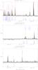 |
Fig. 14 Molecular emission of 12326–6245 around 290 GHz. The best-fit synthetic spectrum is overplotted (solid line). |
 |
Fig. 15 Molecular emission of 12326–6245 around 338 GHz. The best-fit synthetic spectrum is overplotted (solid line). |
This publication is based on data acquired with the Atacama Pathfinder Experiment (APEX). APEX is a collaboration between the Max-Planck-Institut für Radioastronomie, the European Southern Observatory and the Onsala Space Observatory.
Here and below we designate series of lines close together in frequency. The first and second numbers are upper and lower values of the total angular momentum quantum number J of the individual transitions of the series that have different projected angular momentum (K) values.
Acknowledgments
The authors thank an anonymous referee for useful comments. Paola Caselli and Malcolm Walmsley provided additional discussion and comments, which helped to improve the paper. We thank the staff at the APEX and ATCA telescopes and the people who maintain the CDMS and JPL molecular spectroscopy databases. C. Dedes acknowledges financial support from the Studienstiftung des Deutschen Volkes and the International Max Planck Research School for Astronomy and Astrophysics during her thesis work. S. Thorwirth acknowledges support by the Deutsche Forschungsgemeinschaft (TH 1301/3-1). This research has made use of NASA’s Astrophysics Data System and the NASA/ IPAC Infrared Science Archive, which is operated by the Jet Propulsion Laboratory, California Institute of Technology, under contract with the National Aeronautics and Space Administration.
References
- Araya, E., Hofner, P., Kurtz, S., Bronfman, L., & DeDeo, S. 2005, ApJS, 157, 279 [NASA ADS] [CrossRef] [Google Scholar]
- Beltrán, M. T., Brand, J., Cesaroni, R., et al. 2006, A&A, 447, 221 [NASA ADS] [CrossRef] [EDP Sciences] [MathSciNet] [Google Scholar]
- Benjamin, R. A., Churchwell, E., Babler, B. L., et al. 2003, PASP, 115, 953 [NASA ADS] [CrossRef] [Google Scholar]
- Beuther, H., Schilke, P., Menten, K. M., et al. 2002, ApJ, 566, 945 [NASA ADS] [CrossRef] [Google Scholar]
- Beuther, H., Zhang, Q., Sridharan, T. K., Lee, C.-F., & Zapata, L. A. 2006, A&A, 454, 221 [NASA ADS] [CrossRef] [EDP Sciences] [Google Scholar]
- Beuther, H., Zhang, Q., Bergin, E. A., & Sridharan, T. K. 2009, AJ, 137, 406 [NASA ADS] [CrossRef] [Google Scholar]
- Bisschop, S. E., Jørgensen, J. K., van Dishoeck, E. F., & de Wachter, E. B. M. 2007, A&A, 465, 913 [NASA ADS] [CrossRef] [EDP Sciences] [Google Scholar]
- Bronfman, L., Nyman, L.-A., & May, J. 1996, A&AS, 115, 81 [NASA ADS] [Google Scholar]
- Carey, S. J., Noriega-Crespo, A., Mizuno, D. R., et al. 2006, BAAS, 38, 1023 [NASA ADS] [Google Scholar]
- Caselli, P., Hasegawa, T. I., & Herbst, E. 1993, ApJ, 408, 548 [NASA ADS] [CrossRef] [Google Scholar]
- Caswell, J. L. 1998, MNRAS, 297, 215 [NASA ADS] [CrossRef] [Google Scholar]
- Caswell, J. L. 2001, MNRAS, 326, 805 [NASA ADS] [CrossRef] [Google Scholar]
- Cesaroni, R., Olmi, L., Walmsley, C. M., Churchwell, E., & Hofner, P. 1994, ApJ, 435, L137 [NASA ADS] [CrossRef] [Google Scholar]
- Charnley, S. B., Tielens, A. G. G. M., & Millar, T. J. 1992, ApJ, 399, L71 [NASA ADS] [CrossRef] [Google Scholar]
- Chin, Y.-N., Henkel, C., Whiteoak, J. B., Langer, N., & Churchwell, E. B. 1996, A&A, 305, 960 [NASA ADS] [Google Scholar]
- Churchwell, E., Walmsley, C. M., & Wood, D. O. S. 1992, A&A, 253, 541 [NASA ADS] [Google Scholar]
- Comito, C., Schilke, P., Phillips, T. G., et al. 2005, ApJS, 156, 127 [NASA ADS] [CrossRef] [Google Scholar]
- Cyganowski, C. J., Whitney, B. A., Holden, E., et al. 2008, AJ, 136, 2391 [NASA ADS] [CrossRef] [Google Scholar]
- Egan, M. P., Price, S. D., & Kraemer, K. E. 2003, BAAS, 35, 1301 [NASA ADS] [Google Scholar]
- Faúndez, S., Bronfman, L., Garay, G., et al. 2004, A&A, 426, 97 [NASA ADS] [CrossRef] [EDP Sciences] [Google Scholar]
- Garay, G., Brooks, K. J., Mardones, D., & Norris, R. P. 2006, ApJ, 651, 914 [NASA ADS] [CrossRef] [Google Scholar]
- Güsten, R., Nyman, L. Å., Schilke, P., et al. 2006, A&A, 454, L13 [NASA ADS] [CrossRef] [EDP Sciences] [Google Scholar]
- Hatchell, J., Thompson, M. A., Millar, T. J., & MacDonald, G. H. 1998, A&AS, 133, 29 [NASA ADS] [CrossRef] [EDP Sciences] [Google Scholar]
- Henning, T., Lapinov, A., Schreyer, K., Stecklum, B., & Zinchenko, I. 2000, A&A, 364, 613 [NASA ADS] [Google Scholar]
- Heyminck, S., Kasemann, C., Güsten, R., de Lange, G., & Graf, U. U. 2006, A&A, 454, L21 [NASA ADS] [CrossRef] [EDP Sciences] [Google Scholar]
- Hildebrand, R. H. 1983, QJRAS, 24, 267 [NASA ADS] [Google Scholar]
- Hill, T., Burton, M. G., Minier, V., et al. 2005, MNRAS, 363, 405 [NASA ADS] [CrossRef] [Google Scholar]
- Högbom, J. A. 1974, A&AS, 15, 417 [Google Scholar]
- Kalberla, P. M. W., Dedes, L., Kerp, J., & Haud, U. 2007, A&A, 469, 511 [NASA ADS] [CrossRef] [EDP Sciences] [Google Scholar]
- Klein, B., Philipp, S. D., Krämer, I., et al. 2006, A&A, 454, L29 [NASA ADS] [CrossRef] [EDP Sciences] [Google Scholar]
- Kumar, M. S. N., & Grave, J. M. C. 2007, A&A, 472, 155 [NASA ADS] [CrossRef] [EDP Sciences] [Google Scholar]
- Leurini, S., Hieret, C., Thorwirth, S., et al. 2008, A&A, 485, 167 [NASA ADS] [CrossRef] [EDP Sciences] [Google Scholar]
- Liu, S.-Y. 2005, in Astrochemistry: Recent Successes and Current Challenges, ed. D. C. Lis, G. A. Blake, & E. Herbst, IAU Symp., 231, 217 [Google Scholar]
- MacDonald, G. H., Gibb, A. G., Habing, R. J., & Millar, T. J. 1996, A&AS, 119, 333 [NASA ADS] [CrossRef] [EDP Sciences] [Google Scholar]
- MacLaren, I., Richardson, K. M., & Wolfendale, A. W. 1988, ApJ, 333, 821 [NASA ADS] [CrossRef] [Google Scholar]
- MacLeod, G. C., Scalise, E. J., Saedt, S., Galt, J. A., & Gaylard, M. J. 1998, AJ, 116, 1897 [NASA ADS] [CrossRef] [Google Scholar]
- Mangum, J. G., & Wootten, A. 1993, ApJS, 89, 123 [NASA ADS] [CrossRef] [Google Scholar]
- Mangum, J. G., Wooten, A., Wadiak, E. J., & Loren, R. B. 1990, ApJ, 348, 542 [NASA ADS] [CrossRef] [Google Scholar]
- Miettinen, O., Harju, J., Haikala, L. K., & Pomrén, C. 2006, A&A, 460, 721 [NASA ADS] [CrossRef] [EDP Sciences] [Google Scholar]
- Molinari, S., Brand, J., Cesaroni, R., & Palla, F. 2000, A&A, 355, 617 [NASA ADS] [Google Scholar]
- Molinari, S., Testi, L., Rodríguez, L. F., & Zhang, Q. 2002, ApJ, 570, 758 [NASA ADS] [CrossRef] [Google Scholar]
- Motte, F., Andre, P., & Neri, R. 1998, A&A, 336, 150 [NASA ADS] [Google Scholar]
- Mueller, K. E., Shirley, Y. L., Evans, II, N. J., & Jacobson, H. R. 2002, ApJS, 143, 469 [NASA ADS] [CrossRef] [Google Scholar]
- Müller, H. S. P., Schlöder, F., Stutzki, J., & Winnewisser, G. 2005, J. Molec. Struct., 742, 215 [CrossRef] [Google Scholar]
- Müller, H. S. P., Thorwirth, S., Roth, D. A., & Winnewisser, G. 2001, A&A, 370, L49 [NASA ADS] [CrossRef] [EDP Sciences] [Google Scholar]
- Olmi, L., Cesaroni, R., & Walmsley, C. M. 1993, A&A, 276, 489 [NASA ADS] [Google Scholar]
- Olmi, L., Cesaroni, R., Hofner, P., et al. 2003, A&A, 407, 225 [NASA ADS] [CrossRef] [EDP Sciences] [Google Scholar]
- Ossenkopf, V., & Henning, T. 1994, A&A, 291, 943 [NASA ADS] [Google Scholar]
- Panagia, N. 1973, AJ, 78, 929 [NASA ADS] [CrossRef] [Google Scholar]
- Pickett, H. M., Poynter, I. R. L., Cohen, E. A., et al. 1998, J. Quant. Spec. Radiat. Transf., 60, 883 [Google Scholar]
- Purcell, C. R., Balasubramanyam, R., Burton, M. G., et al. 2006, MNRAS, 367, 553 [NASA ADS] [CrossRef] [Google Scholar]
- Reid, M. J., Argon, A. L., Masson, C. R., Menten, K. M., & Moran, J. M. 1995, ApJ, 443, 238 [NASA ADS] [CrossRef] [Google Scholar]
- Risacher, C., Vassilev, V., Monje, R., et al. 2006, A&A, 454, L17 [NASA ADS] [CrossRef] [EDP Sciences] [Google Scholar]
- Rodgers, S. D., & Charnley, S. B. 2001, ApJ, 546, 324 [Google Scholar]
- Schilke, P., Comito, C., Thorwirth, S., et al. 2006, A&A, 454, L41 [NASA ADS] [CrossRef] [EDP Sciences] [Google Scholar]
- Schilke, P., Phillips, T. G., & Mehringer, D. M. 1999, in The Physics and Chemistry of the Interstellar Medium, Proceedings of the 3rd Cologne-Zermatt Symposium, held in Zermatt, September 22−25, 1998, ed. V. Ossenkopf, J. Stutzki, & G. Winnewisser, GCA-Verlag Herdecke, 330 [Google Scholar]
- Shirley, Y. L., Evans, II, N. J., Young, K. E., Knez, C., & Jaffe, D. T. 2003, ApJS, 149, 375 [NASA ADS] [CrossRef] [Google Scholar]
- Siringo, G., Kreysa, E., Kovács, A., et al. 2009, A&A, 497, 945 [NASA ADS] [CrossRef] [EDP Sciences] [Google Scholar]
- Sridharan, T. K., Beuther, H., Schilke, P., Menten, K. M., & Wyrowski, F. 2002, ApJ, 566, 931 [NASA ADS] [CrossRef] [Google Scholar]
- Sutton, E. C., Peng, R., Danchi, W. C., et al. 1995, ApJS, 97, 455 [NASA ADS] [CrossRef] [Google Scholar]
- Urquhart, J. S., Busfield, A. L., Hoare, M. G., et al. 2007a, A&A, 461, 11 [NASA ADS] [CrossRef] [EDP Sciences] [Google Scholar]
- Urquhart, J. S., Busfield, A. L., Hoare, M. G., et al. 2007b, A&A, 474, 891 [NASA ADS] [CrossRef] [EDP Sciences] [Google Scholar]
- Van der Tak, F. F. S., Boonman, A. M. S., Braakman, R., & van Dishoeck, E. F. 2003, A&A, 412, 133 [NASA ADS] [CrossRef] [EDP Sciences] [Google Scholar]
- Viti, S., Collings, M. P., Dever, J. W., McCoustra, M. R. S., & Williams, D. A. 2004, MNRAS, 354, 1141 [NASA ADS] [CrossRef] [Google Scholar]
- Walsh, A. J., Hyland, A. R., Robinson, G., & Burton, M. G. 1997, MNRAS, 291, 261 [NASA ADS] [CrossRef] [Google Scholar]
- Walsh, A. J., Burton, M. G., Hyland, A. R., & Robinson, G. 1998, MNRAS, 301, 640 [NASA ADS] [CrossRef] [Google Scholar]
- Williams, S. J., Fuller, G. A., & Sridharan, T. K. 2004, A&A, 417, 115 [NASA ADS] [CrossRef] [EDP Sciences] [Google Scholar]
- Wilson, T. L., & Rood, R. 1994, ARA&A, 32, 191 [NASA ADS] [CrossRef] [Google Scholar]
- Wouterloot, J. G. A., Henkel, C., Brand, J., & Davis, G. R. 2008, A&A, 487, 237 [NASA ADS] [CrossRef] [EDP Sciences] [Google Scholar]
- Wu, Y., Wei, Y., Zhao, M., et al. 2004, A&A, 426, 503 [NASA ADS] [CrossRef] [EDP Sciences] [Google Scholar]
- Wyrowski, F., Schilke, P., Walmsley, C. M., & Menten, K. M. 1999, ApJ, 514, L43 [NASA ADS] [CrossRef] [Google Scholar]
- Wyrowski, F., Menten, K. M., Schilke, P., et al. 2006, A&A, 454, L91 [NASA ADS] [CrossRef] [EDP Sciences] [Google Scholar]
- Zinchenko, I., Henkel, C., & Mao, R. Q. 2000, A&A, 361, 1079 [NASA ADS] [Google Scholar]
All Tables
Peak coordinates of the 1.2 mm dust continuum data, distances and IRAS luminosities of the three hot core sources (see text).
Properties of 16065−5158 (–62.2 km s-1 ) as derived from LTE modeling of CH3CN , CH3OH , H2COand SO2 .
All Figures
|
Fig. 1 Maps of the HCO + (4−3) line for 12326−6245 (top), 16060−5146 (center) and 16065−5158 (bottom). The (0,0) positions correspond to the 1.2 mm peak positions of Faúndez (2004) listed in Table 1. At each offset position, the velocity and Tmb temperature scales go from −100−20 km s-1 and −5−25 K, −150−0 km s-1 and −5−20 K and −120−0 km s-1 and −5−20 K respectively for 12326−6245, 16060−5146 and 16065−5158. |
| In the text | |
|
Fig. 2 Maps of the CO(3−2) line for 12326−6245 (top), 16060−5146 (middle) and 16065−5158 (bottom). The (0,0) positions correspond to the 1.2 mm peak positions of Faúndez (2004) listed in Table 1. The velocity and Tmb temperature scales go from −100−20 km s-1 and −5−60 K, −150−0 km s-1 and −5−50 K and −120−0 km s-1 and −5−60 K respectively for 12326−6245, 16060−5146 and 16065−5158. |
| In the text | |
|
Fig. 3 C17O(3−2), CO(3−2), CO(4−3) and CO(7−6) transitions. While C17O (3−2) is observed on the peak positions in 16065−5158 (top), 16060−5146 (middle) and 12326−6245 (bottom), the spectra of the remaining transitions were produced by averaging all the spectra taken at the map positions. The dashed line marks the zero level. |
| In the text | |
|
Fig. 4 CH3CN(16−15) data at 294 GHz. We show in blue the synthetic model spectrum (see Tables 29, 30). Note that the spectra for the three sources have been observed with different frequency setups, therefore the SO2 line from the image sidebands appears at different frequencies. The rest frequencies of the |
| In the text | |
|
Fig. 5 LABOCA 870 μm emission (shown as contours), starting from 5σ and continuing in multiples of 1.4σ (see Table 14). The yellow crosses mark the sub-cores in 16060−5146 and 16065−5158. The LABOCA beam is shown as green circle in the lower left of the image. The three-color image shows 3.6 (blue), 4.5 (green) and 8 μm (red) emission from the Spitzer GLIMPSE survey. |
| In the text | |
|
Fig. 6 ATCA 3 mm continuum data (solid lines) top 16060−5146 (contour steps −3, 3, 5, 7...σ, with σ = 0.1 Jy/beam), middle 16065−5158 (contour steps −3, 3, 5, 7...σ, with σ = 8 mJy/beam) and bottom 12326−6245 (contour steps −3, 3, 5, 7...σ, with σ = 0.14 Jy/beam). The synthesized ATCA beam is shown in the lower left corner. LABOCA 870 μm continuum is shown in gray-scales. Symbols: red: radio continuum (Urquhart et al. 2007), blue: OH maser positions, green: offsets of the APEX line observations, turquoise: IRAS position, yellow: CH3OHmaser (Caswell et al. 1998). |
| In the text | |
|
Fig. 7 Zoom-in of the Spitzer GLIMPSE composite image of 3.6, 4.5 and 8 μm emission. LABOCA 870 μm emission is shown as contours, starting from 5σ. The small blue circles and crosses mark the position of the 6 cm and 3.6 cm continuum (Urquhart et al. 2007). 16060–5146: the blue boxes show the location of the ATCA 3 mm continuum emission (marked “a” and “b”). 16065−5158: the cross and circle marking the radio continuum emission are shown in white. |
| In the text | |
|
Fig. 8 Spectrum of 12326−6145. The synthetic model spectrum of CH3OH (7–6) is shown in red. In the upper plot (vt = 1), the synthetic spectrum of the torsionally excited CH3OHtransitions (red) is shown. |
| In the text | |
|
Fig. 9 Spectrum of 12326−6245. The synthetic model spectrum of CH3OH (6–5) is shown in red. In the upper plot (vt = 1), the synthetic spectrum of the torsionally excited CH3OHtransitions (red) is shown. The two lines marked (mirror) in both plots show lines that lie outside the shown frequency range, but were folded into the spectrum owing to imperfect filter edges. |
| In the text | |
|
Fig. 16 Spectral energy distributions for the three sources. The IRAS fluxes (downward pointing triangles) are taken from the high-resolution IRAS Galaxy Atlas (IGA) data. The empty squares and triangles show the MSX and Spitzer GLIMPSE fluxes respectively, the filled circles the ATCA fluxes and the filled triangle and square the bolometer fluxes from SIMBA and LABOCA. |
| In the text | |
|
Fig. 17 Fractional abundances in the three sources for T < 100 K (cold component, top plot) and T > 100 K (hot component, bottom plot). Red triangles show abundances for G34.3+0.15 (Macdonald et al. 1996), green stars for NGC 6334I, blue stars for G327.3-0.6 (both Schilke et al. 2006) and turquoise stars for 17233–3606 (Leurini et al. 2007). The red lines indicate those molecules where the modeling of different transitions resulted in different column densities (see Tables 34 to 33). |
| In the text | |
|
Fig. 10 Molecular emission of 16065–5158 around 290 GHz and 436 GHz. The best-fit synthetic spectrum is overplotted (solid line). |
| In the text | |
|
Fig. 11 Molecular emission of 16065–5158 around 338 GHz. The best-fit synthetic spectrum is overplotted (solid line). |
| In the text | |
|
Fig. 12 Molecular emission of 16060–5146 around 290 GHz and 436 GHz. The best-fit synthetic spectrum is overplotted (solid line). |
| In the text | |
|
Fig. 13 Molecular emission of 16060–5146 around 338 GHz. The best-fit synthetic spectrum is overplotted (solid line). |
| In the text | |
|
Fig. 14 Molecular emission of 12326–6245 around 290 GHz. The best-fit synthetic spectrum is overplotted (solid line). |
| In the text | |
|
Fig. 15 Molecular emission of 12326–6245 around 338 GHz. The best-fit synthetic spectrum is overplotted (solid line). |
| In the text | |
Current usage metrics show cumulative count of Article Views (full-text article views including HTML views, PDF and ePub downloads, according to the available data) and Abstracts Views on Vision4Press platform.
Data correspond to usage on the plateform after 2015. The current usage metrics is available 48-96 hours after online publication and is updated daily on week days.
Initial download of the metrics may take a while.