| Issue |
A&A
Volume 525, January 2011
|
|
|---|---|---|
| Article Number | A96 | |
| Number of page(s) | 11 | |
| Section | The Sun | |
| DOI | https://doi.org/10.1051/0004-6361/201015534 | |
| Published online | 03 December 2010 | |
Thermal conduction effects on the kink instability in coronal loops
1
Centre for Fusion, Space and Astrophysics, Department of PhysicsUniversity
of Warwick,
Coventry
CV4 7AL,
UK
e-mail: This email address is being protected from spambots. You need JavaScript enabled to view it.
; This email address is being protected from spambots. You need JavaScript enabled to view it.
2
School of Mathematics and Statistics, St Andrews University,
St Andrews,
KY16 9SS,
UK
e-mail: This email address is being protected from spambots. You need JavaScript enabled to view it.
Received:
5
August
2010
Accepted:
20
October
2010
Abstract
Context. Heating of the solar corona by nanoflares, which are small transient events in which stored magnetic energy is dissipated by magnetic reconnection, may occur as the result of the nonlinear phase of the kink instability (Hood et al. 2009). Because of the high temperatures reached through these reconnection events, thermal conduction cannot be ignored in the evolution of the kink instability.
Aims. To study the effect of thermal conduction on the nonlinear evolution of the kink instability of a coronal loop. To assess the efficiency of loop heating and the role of thermal conduction, both during the kink instability and for the long time evolution of the loop.
Methods. Numerically solve the 3D nonlinear magnetohydrodynamic equations to simulate the evolution of a coronal loop that is initially in an unstable equilibrium. The initial state has zero net current. A comparison is made of the time evolution of the loop with thermal conduction and without thermal conduction.
Results. Thermal conduction along magnetic field lines reduces the local temperature. This leads to temperatures that are an order of magnitude lower than those obtained in the absence of thermal conductivity. Consequently, different spectral lines are activated with and without the inclusion of thermal conduction, which have consequences for observations of solar corona loops. The conduction process is also important on the timescale of the fast magnetohydrodynamic phenomena. It reduces the kinetic energy released by an order of magnitude.
Conclusions. Thermal conduction plays an essential role in the kink instability of coronal loops and cannot be ignored in the forward modelling of such loops.
Key words: Sun: corona / Sun: flares / magnetohydrodynamics (MHD) / magnetic fields / plasmas / magnetic reconnection
© ESO, 2010
1. Introduction
Nanoflares are thought to play a significant role in the heating of the solar corona (Parker 1988). The proposal is that they provide many small events that are distributed across the corona, releasing magnetic energy and maintaining the temperature of the X-ray corona. Evidence suggests that large flares are triggered by reconnection events (Schrijver 2009). Given the universal scaling laws for the physical parameters of flare-like processes (Aschwanden & Parnell 2002), it is reasonable to assume that reconnection events are also the trigger for microflares and nanoflares (Jess et al. 2010).
The magnetic field must be twisted for the ideal magnetohydrodynamic (MHD) kink instability to occur. It is usually assumed that the magnetic energy of coronal loops is increased through footpoint motion, where the magnetic fields are line-tied in the denser photosphere (Gerrard et al. 2004). It is known that for slow photospheric motion the line-tied approximation may break down (Hood et al. 1989; Grappin et al. 2008), so that highly stressed magnetic fields need additional processes to obtain high magnetic energy levels. Such processes include flux emergence (Arber et al. 2007; Lites 2009) or submergence (Kálmán 2001; Iida et al. 2010). In this paper the initial state of the coronal loop is an unstable equilibrium and we do not consider the process by which the magnetic field became twisted.
A reconnection event occurs when the magnetic field relaxes to a lower energy state by a realignment of field lines. Browning et al. (2008) showed that the trigger for such a relaxation event can be the onset of an ideal kink instability. For a typical coronal plasma, the timescales for heat conduction are normally much longer than those for ideal MHD instabilities (Hood 1990). Hence analytical and numerical studies of the ideal kink instability in the low-β plasma of the solar corona have omitted thermal conductivity, where the plasma β is the ratio of gas pressure to magnetic pressure. It is generally acknowledged that when the long time evolution of coronal loops is investigated, thermal conductivity should be included to investigate the loop behaviour after the ideal MHD instabilities have relaxed the magnetic field configuration to a lower energy state (Torricelli-Ciamoni et al. 1987; Van der Linden & Goossens 1991; Soler et al. 2008).
The timescale of MHD processes, including the kink instability, can be roughly estimated as
the Alfvén transit time along the loop. For a loop with an average magnetic field of
B0 = 50 G, an electron density of
ne = 1014 m-3 and loop length of
L0 = 40 Mm this gives the MHD timescale as
τMHD ≃ 2 s. From Eqs. (4) and (9) below, the thermal
conduction timescale (in SI units) is  , where
T0 is the loop plasma temperature. For
T0 = 1 MK this gives
τκ ≃ 80 s. Thus for such coronal loops the
MHD timescale is of the order of seconds while that for thermal conduction is of the order
of minutes. It is estimates of these timescales that have lead to the widely held view that
for the kink instability it is safe to ignore thermal conduction, which is only needed for
the longer timescale evolution of the loop. Recent numerical simulations of the ideal kink
instability (Hood et al. 2009) showed that magnetic
reconnection events, occurring during the nonlinear phase of the ideal kink instability,
lead to heating. Strong current sheets form at the reconnection sites, which drives
temperatures up to values of 100 MK by means of Ohmic heating. These high temperatures are
also on scales less than the whole loop length. Thus L0 is
reduced and T0 increased in the estimation of
τκ and
τκ < τMHD.
In this case thermal conduction may also be important during the initial MHD driven kink
instability.
, where
T0 is the loop plasma temperature. For
T0 = 1 MK this gives
τκ ≃ 80 s. Thus for such coronal loops the
MHD timescale is of the order of seconds while that for thermal conduction is of the order
of minutes. It is estimates of these timescales that have lead to the widely held view that
for the kink instability it is safe to ignore thermal conduction, which is only needed for
the longer timescale evolution of the loop. Recent numerical simulations of the ideal kink
instability (Hood et al. 2009) showed that magnetic
reconnection events, occurring during the nonlinear phase of the ideal kink instability,
lead to heating. Strong current sheets form at the reconnection sites, which drives
temperatures up to values of 100 MK by means of Ohmic heating. These high temperatures are
also on scales less than the whole loop length. Thus L0 is
reduced and T0 increased in the estimation of
τκ and
τκ < τMHD.
In this case thermal conduction may also be important during the initial MHD driven kink
instability.
The structure of the paper starts with a description of the model used, which includes the physics incorporated into the model, the initial state of the coronal loop and the numerical procedures. It then continues by presenting the simulation results by comparing the energy budget, temperature and magnetic field configuration of a simulation where thermal conduction is included with a simulation where it is omitted. The paper concludes by summarising these results and their implications for observations of the kink instability in the corona.
2. Numerical model and procedure
2.1. Physical model
The time evolution of a coronal loop is studied, with its footpoints in the photosphere.
Nonlinear three-dimensional simulations are performed using the MHD Lagrangian-remap code,
Lare3d, as described by Arber et al. (2001). It
solves the resistive MHD equations 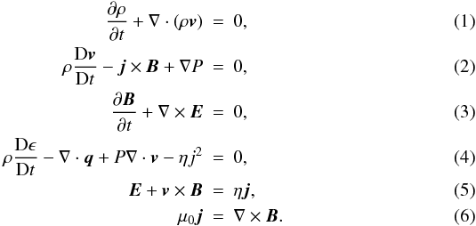 Here
D/Dt is the advective derivative, ρ the mass
density,
Here
D/Dt is the advective derivative, ρ the mass
density,  (7)the
pressure, with kB the Boltzmann constant, T
the temperature, and
(7)the
pressure, with kB the Boltzmann constant, T
the temperature, and  the reduced mass where
  is the average mass of an ion in the plasma.
 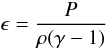 (8)is
the specific internal energy density, γ = 5/3 the ratio of specific
heats, v the bulk velocity of the plasma,
B the magnetic field, j
the current density and μ0 is the vacuum permeability. The
heat flux vector q is
(8)is
the specific internal energy density, γ = 5/3 the ratio of specific
heats, v the bulk velocity of the plasma,
B the magnetic field, j
the current density and μ0 is the vacuum permeability. The
heat flux vector q is 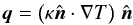 (9)with
 and
κ = κ0T5/2,
where κ0 = 10-11. Thus the thermal conduction along
the magnetic field is the classical Spitzer-Härm (1953), or Braginskii, conductivity with log Λ = 18.4. This is a common coronal
approximation. Note that this form of thermal conduction assumes that the mean free path
of the hot electrons remains small compared to the macroscopic scale lengths. It also
assumes that the dominant energy release is thermal and hence the results in this paper
cannot be simply applied to large flares where significant non-thermal electron energies
are generated. Thus the model presented here can only be valid for nanoflares and
microflares, where the energy released is likely to be thermal and there is no direct
evidence of significant electron acceleration. Assessing the validity of the Spitzer-Härm
conductivity would require a kinetic treatment and is beyond the scope of these fluid
simulations. Bell et al. (1981) have shown that the
Spitzer-Härm thermal conductivity may begin to break down when the mean free path of
electrons is greater than just one percent of the temperature scale length. In more recent
coronal studies West et al. (2008) looked at the
effect of nonlocal electrons on thermal conduction. They showed that these electrons
lengthen cooling times considerably. However, they also showed that in the parameter space
discussed in this paper, the Spitzer-Härm formalism is a very good approximation even when
nonlocal effects are considered.
and
κ = κ0T5/2,
where κ0 = 10-11. Thus the thermal conduction along
the magnetic field is the classical Spitzer-Härm (1953), or Braginskii, conductivity with log Λ = 18.4. This is a common coronal
approximation. Note that this form of thermal conduction assumes that the mean free path
of the hot electrons remains small compared to the macroscopic scale lengths. It also
assumes that the dominant energy release is thermal and hence the results in this paper
cannot be simply applied to large flares where significant non-thermal electron energies
are generated. Thus the model presented here can only be valid for nanoflares and
microflares, where the energy released is likely to be thermal and there is no direct
evidence of significant electron acceleration. Assessing the validity of the Spitzer-Härm
conductivity would require a kinetic treatment and is beyond the scope of these fluid
simulations. Bell et al. (1981) have shown that the
Spitzer-Härm thermal conductivity may begin to break down when the mean free path of
electrons is greater than just one percent of the temperature scale length. In more recent
coronal studies West et al. (2008) looked at the
effect of nonlocal electrons on thermal conduction. They showed that these electrons
lengthen cooling times considerably. However, they also showed that in the parameter space
discussed in this paper, the Spitzer-Härm formalism is a very good approximation even when
nonlocal effects are considered.
Equations (2) and (4) use a single isotropic pressure, which is most easily justified if the ions and electrons are the same temperature. For the densities and temperatures considered here, the temperature equilibration time may be of order minutes, suggesting the need for a two fluid approach. However, since only low-β plasmas will be considered, the overall dynamics, i.e. magnetic field and electron temperature, are expected to be well represented by a single-fluid model.
Shock viscosity is included as a heating term in these simulations, as described in Arber et al. (2001), as is Ohmic heating. The only energy transport included is thermal conduction. For the coronal temperatures considered here, the thermal conduction will dominate over optically thin radiative losses. In the transition region such radiative losses will become important but this is outside of our computational domain. We are, therefore, assuming that the thermal conduction out of our computational domain will lead to radiation from the transition region/chromosphere but that this will not significantly feedback on to our coronal solution.
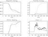 |
Fig. 1 Plots of the magnetic energy, thermal energy, Ohmic heating and the maximum current density as functions of time. The solid line is with thermal conduction and the dotted line is without conduction. The final dimensional values with thermal conductivity are 10.3 PJ for magnetic energy, 8.1 TJ for thermal energy, 28.3 TJ for Ohmic heating and 20 mA for max(j). |
 (10)Here
L0 is a characteristic length,
B0 the characteristic magnetic field strength and
ρ0 the characteristic mass density. In the absence of
thermal conductivity, the normalised equations are given by (1) to (6) and (8) with μ0 = 1 and
the resistivity is replaced by
η → η/(μ0L0v0),
i.e. the resistivity is replaced by the inverse Lundquist number.
(10)Here
L0 is a characteristic length,
B0 the characteristic magnetic field strength and
ρ0 the characteristic mass density. In the absence of
thermal conductivity, the normalised equations are given by (1) to (6) and (8) with μ0 = 1 and
the resistivity is replaced by
η → η/(μ0L0v0),
i.e. the resistivity is replaced by the inverse Lundquist number.
With this choice of normalisation the heat flux still has the form given in Eq. (9) but the normalised thermal conductivity is
now given by  (11)where T
now refers to the normalised temperature. Note that throughout this paper the pressure is
normalised to the magnetic pressure and the temperature is similarly normalised with
respect to Alfvén speeds. Therefore, after normalisation both the pressure and temperature
for a low-β plasma will be of order 1/β.
(11)where T
now refers to the normalised temperature. Note that throughout this paper the pressure is
normalised to the magnetic pressure and the temperature is similarly normalised with
respect to Alfvén speeds. Therefore, after normalisation both the pressure and temperature
for a low-β plasma will be of order 1/β.
The resistivity is of the form  (12)where
ηb is the uniform background resistivity and
η0 an anomalous resistivity that comes into play only when
the magnitude of the current exceeds the critical value
jc = 5. Figure 1 gives
the time evolution of max(j) in the simulation. It shows that at around
time 80, η0 switches on in the regions where
| j | ≥ jc and stays on for the duration
of the simulation. This means that η0 is activated as soon as
the kink instability occurs in the simulation. Unless otherwise stated
ηb = 0, so that only anomalous resistivity is applied.
Gravity is set to zero and we ignore radiation.
(12)where
ηb is the uniform background resistivity and
η0 an anomalous resistivity that comes into play only when
the magnitude of the current exceeds the critical value
jc = 5. Figure 1 gives
the time evolution of max(j) in the simulation. It shows that at around
time 80, η0 switches on in the regions where
| j | ≥ jc and stays on for the duration
of the simulation. This means that η0 is activated as soon as
the kink instability occurs in the simulation. Unless otherwise stated
ηb = 0, so that only anomalous resistivity is applied.
Gravity is set to zero and we ignore radiation.
2.2. Initial conditions
As in Hood et al. (2009), the initial state is
chosen to be a force-free equilibrium unstable to an ideal MHD kink instability. Hence the
magnetic field satisfies the equation
 (13)The equilibrium
is a modification of the model described by Browning and Van der Linden (2003) and consists of two regions. For
r < 1 we have
(13)The equilibrium
is a modification of the model described by Browning and Van der Linden (2003) and consists of two regions. For
r < 1 we have 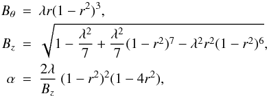 (14)and
for r ≥ 1
(14)and
for r ≥ 1 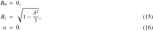 This
magnetic field ensures that α has a sign change at
r = 0.5. The requirement that
This
magnetic field ensures that α has a sign change at
r = 0.5. The requirement that  restricts the values of λ, so that
 . The simulation results
presented in this paper were obtained with a value of λ = 1.8. The
initial density and temperature are chosen to be constant. The normalised density equals
1, while the normalised temperature correspond to 104 K. Hence the initial
coronal atmosphere is assumed cold and fixed at a temperature corresponding to the upper
chromosphere or low transition region.
. The simulation results
presented in this paper were obtained with a value of λ = 1.8. The
initial density and temperature are chosen to be constant. The normalised density equals
1, while the normalised temperature correspond to 104 K. Hence the initial
coronal atmosphere is assumed cold and fixed at a temperature corresponding to the upper
chromosphere or low transition region.
2.3. Numerical procedure
The dynamics of the coronal loops are studied in Cartesian geometry, neglecting field line curvature. The x and y boundaries are at ±2 while the z boundaries are at ±10. This means the computational domain has sizes Lx = Ly = 4 and Lz = 20. The x and y boundaries are reflective, while line-tied boundaries are employed at the z boundaries. This means that at the loop ends the velocity is held zero and the temperature is fixed at 104 K, the value of the initial background temperature, while the temperature gradient is allowed to vary. Hence, there will be a heat flux across the ends of the loop. Ideally a transition region should be included at the z boundaries, with the boundary temperature fixed to chromospheric values. However, the 3D model used here would not be able to resolve the temperature gradients with realistic optically thin radiation. Also, this paper considers the heating process through nanoflares and relaxation, which result in a smaller heat flux through the boundary than is the case for large flares.
The initial equilibrium condition is a loop of normalised radius 1, so that the aspect ratio of the initial cylinder is 20, similar to Browning & Van der Linden (2003), Browning et al. (2008) and Hood et al. (2009). Each simulation was run with grid resolutions 1282 × 256 and 2562 × 512. Similar results are obtained with the two resolutions, with more fine structure shown in the higher resolution. We have tested the numerical result by using a lower resolution, which also gave qualitatively similar results.
The thermal conduction term in Eq. (4) is treated implicitly. This is done by a parallel, red-black ordered, SOR scheme with an over-relaxation parameter of 1.6. Iteration is stopped when the mean fractional error in the temperature is 10-3. The largest local temperature errors are of order 1%. Since the plasma remains predominantly low β, increasing the accuracy of the SOR routine through more iterations has little effect on the solution. A maximum allowable error of 1% in temperature was chosen to balance runtime with accuracy.
3. Simulation results
The results presented in this paper were obtained by using the normalisation L0 = 106 m, B0 = 5 × 10⁻³ T, i.e. 50 Gauss, and ρ0 = 1014 × 1.6726 × 10-27 = 1.6726 × 10⁻¹³ kg m-3. This leads to a time normalisation of t0 = 0.09 s and a temperature normalisation of T0 = 1.44 × 10¹⁰ K. When another normalisation is used, it will be clearly stated.
3.1. Global energy budget
The overall picture of heating due to the kink instability in a coronal loop is that the kink instability drives magnetic field into a current sheet. Here it reconnects releasing energy until the kink instability, and subsequent motion, relaxes the loop to a stable configuration. Since the drive for the magnetic energy release is an unstable magnetic field configuration and the plasma β is low in the corona, the plasma thermal pressure is not expected to play a dominant role in the magnetic energy release. This is confirmed in Fig. 1 which shows the magnetic energy released both with and without thermal conduction. The coronal plasma has a low plasma β, so that magnetic processes dominate the physics. The current density is calculated from the deformation of the magnetic field through Eq. (6), so that its evolution is similar with and without thermal conductivity. As a result, the Ohmic heating in the coronal loop is not very sensitive to the inclusion of thermal conductivity.
Figure 1 shows that the magnetic energy of the simulations with and without thermal conductivity do not have the same value at the end of the simulations. The final magnetic field will depend on the final thermal pressure and, if the thermal pressure is non-uniform, the resulting magnetic field will not be potential. Since the final thermal pressure is higher for the case without thermal conduction, the final magnetic energy will be subsequently larger. Obviously, if the magnetic field configurations tend to a potential final state, then both cases will converge to the same value, but this only happens after a much longer time.
Thermal energy is almost an order of magnitude lower when thermal conduction is included. The heat is transported along the magnetic field lines away from the points where magnetic reconnection heats the plasma. The field lines are tied to the top and bottom z boundaries, which means that energy escapes the numerical domain through these two planes.
It is instructive to separate the total kinetic energy into components parallel and
perpendicular to the local magnetic field: 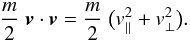 (17)The total kinetic energy
is lower when thermal conduction is included. Figure 2 shows that this is because the contribution of parallel kinetic energy is
reduced while the perpendicular kinetic energy remains of comparable size to that without
thermal conduction. Without thermal conductivity a reconnection event increases the local
temperature, which means the local pressure increases. This drives parallel flows. The
dominant source of the perpendicular kinetic energy is from the kink instability itself
and is thus driven by the unstable magnetic field. When parallel thermal conductivity is
included, thermal energy is transported away from the reconnection site along field lines.
This has the effect of reducing both the maximum pressure and the pressure scale length
along a field line. This reduces the parallel flow, which leads to lower parallel kinetic
energy. In contrast, since the plasma is low β there is little change in
the MHD instability, so that the kinetic energy perpendicular to the magnetic field lines
stay of the same order.
(17)The total kinetic energy
is lower when thermal conduction is included. Figure 2 shows that this is because the contribution of parallel kinetic energy is
reduced while the perpendicular kinetic energy remains of comparable size to that without
thermal conduction. Without thermal conductivity a reconnection event increases the local
temperature, which means the local pressure increases. This drives parallel flows. The
dominant source of the perpendicular kinetic energy is from the kink instability itself
and is thus driven by the unstable magnetic field. When parallel thermal conductivity is
included, thermal energy is transported away from the reconnection site along field lines.
This has the effect of reducing both the maximum pressure and the pressure scale length
along a field line. This reduces the parallel flow, which leads to lower parallel kinetic
energy. In contrast, since the plasma is low β there is little change in
the MHD instability, so that the kinetic energy perpendicular to the magnetic field lines
stay of the same order.
 |
Fig. 2 Plots of the total kinetic energy, as well as its parallel and perpendicular components. These are calculated using v = v ⊥ + v ∥ . The solid line is with thermal conduction and the dotted line is without conduction. With thermal conductivity, the maximum value of the dimensional kinetic energy is 5.828 TJ for the total kinetic energy at time 118, 0.299 TJ for the parallel and 5.542 TJ for the perpendicular components. |
3.2. Temperature evolution
Figure 3 shows profiles of the temperature along a line across the middle of the coronal loop. Plotted are the results with and without conduction. Note that the results with thermal conduction have been multiplied by 10 to fit on the same scale. The results with conduction have a peak temperature that is an order of magnitude lower than when thermal conduction is not included. The reason for this is the more effective temperature transport along magnetic field lines when thermal conductivity is included. Figure 4 shows the temperature profile along magnetic field lines. At time 100 the kink instability has triggered reconnection and the temperature has risen at the reconnection sites. In the simulation without thermal conductivity the temperature rise is extremely localised, while for the case with thermal conductivity the high temperature has spread along the magnetic field lines that pass through the reconnection site. At time 125, both cases show that the higher temperature has spread along the magnetic field lines passing through the reconnection site. However, in the case without thermal conductivity the high temperature is still much more localised than is the case with thermal conductivity.
The temperature increases at the reconnection sites, as is clearly observable in Fig. 3. After reconnection the temperature decreases due to thermal conduction along magnetic field lines. This temperature decrease is seen when times 105, 130 and 160 are compared. Without thermal conduction the temperature decreases between times 105 and 130. This is due to pressure gradients forming at the reconnection sites. The locally hot plasma will have a higher pressure that will drive flows, reducing the temperature.
The temperature profile is also more diffuse when thermal conduction is included. This can be seen more clearly in the filled contour plots of Figs. 5 and 6. The reduction in the peak temperature is easily explained due to thermal conduction along field lines. It is important to note that the spreading of temperature across the loop cross-section is not due to cross-field thermal diffusion. In the central plane of the loop cross-section the magnetic field is predominantly perpendicular to this plane, so parallel thermal conduction is also predominantly out of the plane presented in Figs. 5 and 6. This apparent cross-field thermal diffusion is a result of the combination of parallel thermal conduction and reconnection. As shown in Fig. 7, reconnection untwists the unstable initial field configuration. Reconnection occurs along the loop length and not just in the z = 0 plane. Thus at t = 105, for example, the primary reconnection site in the z = 0 plane is at r ≃ 0.6, as can be seen from the results without thermal conduction (Fig. 5). At t = 105, Fig. 7 shows that as a result of reconnection, points inside r ≃ 0.6 in the z = 0 plane are now connected by field lines to the r ≃ 0.6 reconnection sites at other locations along the loop. Since thermal conduction enhances energy transport along magnetic field lines, the heating at other axial locations at around r ≃ 0.6 is conducted to positions of radius less than 0.6 in the z = 0 plane. Thus the apparent cross-field thermal diffusion in Figs. 5 and 6 is actually the result of parallel thermal conduction from other locations along the loop.
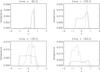 |
Fig. 3 Normalised temperature profiles along the x direction at position y = 0 and z = 0. The solid line is with thermal conduction and the dotted line is without conduction. The temperature obtained with conduction has been multiplied by 10.0 to fit on the same scale as the dotted line. The dimensional values of the maximum temperature with thermal conduction are 8.42 MK at time 90, 18.39 MK at time 105, 9.49 MK at time 130, and 6.73 MK at time 160. |
 |
Fig. 4 Magnetic field lines showing the temperature along them in colour. Results without thermal conduction are labelled (a) and with thermal conduction (b). Note that the colour scale is different for the two cases: red denotes a normalised temperature of 0.02 for (a) and 0.008 for (b). These represent dimensional temperature values of 288.2 MK and 115.3 MK respectively. In both cases blue denotes a normalised temperature of values below 10-5, or equivalently 0.1 MK. |
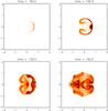 |
Fig. 5 Temperature in the plane perpendicular to the z axis at position z = 0. The temperature was measured for the case without thermal conduction. The colour scale gives white as the initial temperature and dark as max(T) = 2.55 × 10⁻² (dimensional temperature 367.42 MK), which is obtained at time 105. The dotted line in Fig. 3 shows the data along a cut through the centre of the plane along the x direction. |
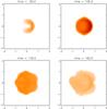 |
Fig. 6 Temperature on the plane perpendicular to the z axis at position z = 0. The temperature was measured for the case with thermal conduction. The colour scale is the same as in Fig. 5. The solid line in Fig. 3 shows the data along a cut through the centre of the plane along the x direction. As in Fig. 3, the temperature was multiplied by 10.0 to fit on the same scale as Fig. 5. |
Figure 7 shows that magnetic reconnection occurs with and without the inclusion of thermal conduction. Individual field lines may be traced to different locations, but overall there is little difference between the results with or without thermal conduction. This is expected, given that the plasma β is very low and magnetic field evolution is therefore largely insensitive to the thermal structure of the loop.
The relaxation of magnetic field lines by the end of the simulations do not exactly match the final state predicted by relaxation theory (also seen in Hood et al. 2009), which can be helical, but the energy released during the kink instability is very close to that predicted by the theory. Given time, the plasma would reach the final relaxed state, but only very slowly.
With the difference in temperature, there is also a difference in the plasma β between the two cases. Without conduction the higher localised heating leads to a maximum plasma β of 0.1 (at time 105). With thermal conduction the maximum plasma β is 8 × 10⁻³.
3.3. Temperature isosurfaces
Figure 3 shows that the temperature maxima decreases when thermal conductivity is included. This has observational consequences in that different spectral lines are activated at different temperatures. The predictable observational signatures of forward models (Arber et al. 1999; Haynes & Arber 2007) are highly dependent on whether thermal conductivity is included or not. In order to obtain observational signatures, the temperature and density must be fed through the instrumental response functions of the various observational platforms. This is beyond the scope of the present paper.
When parallel thermal conduction is included, the heat is conducted along the magnetic field lines away from the local heating source, so that the plasma takes longer to reach high temperatures. This is illustrated in Fig. 8, where isosurfaces for a normalised temperature of 7.5 × 10⁻⁴ are presented. The thermal energy flow along the magnetic field lines is increased with the inclusion of thermal conductivity. This is clearly seen when the simulations with and without conductivity are compared at times 95 and 100 in Fig. 8. Parallel thermal conduction also causes the plasma to cool faster, so that one obtains shorter time intervals during which this temperature isosurface exists, as is evident at time 120 in Fig. 8.
Table 1 shows the lifetime of different isosurfaces for the simulations with thermal conduction included. Here the lifetimes are presented in units of normalised time. The temperatures of each isosurface are all reached at approximately the same time (t ≃ 80). Without thermal conduction these isosurfaces exist at the end of the simulations for all temperatures listed in Table 1, i.e. from 1.4 MK to 15.8 MK. For temperatures above 5.8 MK the simulations with thermal conduction predict that spectral lines sensitive to these temperatures would be visible for at most 7 s. The same simulations without thermal conduction predict all temperatures from 1.4 MK to 15.8 MK would be visible for at least 30 s.
Duration of temperature isosurface visibility.
3.4. The influence of the normalisation
The choice of normalisation parameters B0, ρ0 and L0 are unimportant for resistive MHD, i.e. the equations can be solved in normalised form and values for B0, ρ0 and L0 specified arbitrarily. This is not true for simulations that include thermal conductivity, as this uses the real, physical value for parallel thermal conductivity, as shown in (11). Therefore, testing the effect of thermal conductivity on other loops involves new simulations with different choices for B0, ρ0 and L0. For this test we have deliberately chosen values to minimise the effect of thermal conductivity. By reducing B0 the magnetic energy released is reduced and by increasing ρ0 the heat input from the magnetic energy release generates a lower temperature. Specifically, we have chosen L0 = 106 m, B0 = 2 × 10⁻³ T and ρ0 = 1.67 × 10⁻¹² kg m-3. The results are presented in Fig. 9. In this case the temperature with thermal conduction is half that which is obtained without thermal conduction. Even in this extreme case, in the sense of weak field and high density, one can see the effect of thermal conduction.
Table 2 shows the lifetime of different isosurfaces for the simulations with thermal conduction included. For observations sensitive to temperatures of around 2 MK, thermal conduction reduces the timescale over which this temperature is visible from at least 3 min to at most 8.4 s.
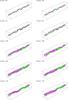 |
Fig. 7 Magnetic field lines drawn from the two end planes: green from z = −10 and pink from z = 10. Results without thermal conduction are labelled (a) and with thermal conduction (b). |
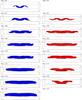 |
Fig. 8 Isosurfaces of the normalised temperature T = 7.5 × 10⁻⁴, with the blue isosurfaces (left hand column) obtained without thermal conduction and the red isosurfaces (right hand column) with thermal conduction. At times 90 and 125 for the case with thermal conduction there is no plasma at this temperature and hence no isosurface is shown. |
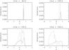 |
Fig. 9 Temperature profiles along the x direction at position y = 0 and z = 0. The solid line is with thermal conduction and the dotted line is without conduction. These results were obtained with the normalisation L0 = 106 m, B0 = 2 × 10⁻³ T and ρ0 = 1.67 × 10⁻¹² kg m-3. This leads to a time normalisation of t0 = 0.7 s and a temperature normalisation of T0 = 2.31 × 10⁸ K. Without thermal conduction the result is independent of the normalisation used, as can be seen when compared to Fig. 3. The dimensional values of max(T) with thermal conduction are 1.92 MK at time 90, 2.12 MK at time 105, 1.57 MK at time 130, and 1.46 MK at time 160. |
4. Conclusions
This paper presents results assessing the importance of thermal conduction in simulations, and hence forward modelling, of kink unstable coronal loops. Since the real thermal conductivity is used, the results are sensitive to the physical parameters of the loop and two loops have been tested. The first assumed a typical magnetic field strength of 50 G and an electron number density of ne = 1014 m-3. To minimise the effects of conduction, the second loop had a magnetic field strength of 20 G and an electron number density of ne = 1015 m-3. These loops will be referred to as the high field and low field loops respectively. From these simulations the main conclusions are:
-
For the high field loop thermal conduction reduces the maximumtemperature by an order of magnitude compared to simulationswith no conduction. For the low field loop the reduction is by afactor of two.
-
For both loops there are clear differences in the time history of temperature isosurfaces when thermal conduction is included, which affect temperature sensitive observations.
-
Thermal conduction affects the evolution even during the rapid MHD timescale of the kink instability. It reduces the parallel kinetic energy, i.e.
 , due to
the reduction in peak temperature and smoothing of the temperature scale length along
magnetic field lines. These combine to reduce the pressure gradient along the field
and hence lead to a reduction of sound wave generation and flows along the field.
, due to
the reduction in peak temperature and smoothing of the temperature scale length along
magnetic field lines. These combine to reduce the pressure gradient along the field
and hence lead to a reduction of sound wave generation and flows along the field.
It is therefore clear from these simulations that any attempt at forward modelling of a comprehensive set of observational signatures of kink unstable coronal loops must include parallel thermal conduction. This will be true for all MHD phenomena in the corona where magnetic energy is converted into thermal energy. Note however, that our model uses the Braginskii parallel thermal conduction, which is only valid for short mean free paths, compared to macroscopic lengths and near Maxwellian distributions. These results cannot therefore be directly applied to large flares where significant non-thermal electron populations are generated.
Acknowledgments
This work was funded in part by the Science and Technology Facilities Council. The computational work was supported by resources made available through Warwick University’s Centre for Scientific Computing.
References
- Arber, T. D., Longbottom, A. W., & Van der Linden, R. A. M. 1999, ApJ, 517, 990 [NASA ADS] [CrossRef] [Google Scholar]
- Arber, T. D., Longbottom, A. W., Gerrard, C. L., & Milne, A. M. 2001, J. Comput. Phys., 171, 151 [NASA ADS] [CrossRef] [Google Scholar]
- Arber, T. D., Haynes, M., & Leake, J. E. 2007, ApJ, 666, 541 [NASA ADS] [CrossRef] [Google Scholar]
- Aschwanden, M. J., & Parnell, C. E. 2002, ApJ, 572, 1048 [NASA ADS] [CrossRef] [Google Scholar]
- Bell, A. R., Evans, R. G., & Nicholas, D. J. 1981, Phys. Rev. Lett., 46, 243 [NASA ADS] [CrossRef] [Google Scholar]
- Browning, P. K., & Van der Linden, R. A. M. 2003, A&A, 400, 355 [NASA ADS] [CrossRef] [EDP Sciences] [Google Scholar]
- Browning, P. K., Gerrard, C., Hood, A. W., Kevis, R., & Van der Linden, R. A. M. 2008, A&A, 485, 837 [NASA ADS] [CrossRef] [EDP Sciences] [Google Scholar]
- Gerrard, C. L., Hood, A. W., & Brown, D. S. 2004, Sol. Phys., 222, 79 [NASA ADS] [CrossRef] [Google Scholar]
- Grappin, R., Aulanier, G., & Pinto, R. 2008, A&A, 490, 353 [NASA ADS] [CrossRef] [EDP Sciences] [Google Scholar]
- Haynes, M., & Arber, T. D. 2007, A&A, 467, 327 [NASA ADS] [CrossRef] [EDP Sciences] [Google Scholar]
- Hood, A. W. 1990, Comp. Phys. Rep., 12, 177 [NASA ADS] [CrossRef] [Google Scholar]
- Hood, A. W., Van der Linden, R. A. M., & Goossens, M. 1989, Sol. Phys., 120, 261 [NASA ADS] [CrossRef] [Google Scholar]
- Hood, A. W., Browning, P. K., & Van der Linden, R. A. M. 2009, A&A, 506, 913 [NASA ADS] [CrossRef] [EDP Sciences] [Google Scholar]
- Iida, Y., Yokoyama, T., & Ichimoto, K. 2010, ApJ, 713, 325 [NASA ADS] [CrossRef] [Google Scholar]
- Jess, D. B., Mathioudakis, M., Browning, P. K., Crockett, P. J., & Keenan, F. P. 2010, ApJ, 712, L111 [NASA ADS] [CrossRef] [Google Scholar]
- Kálmán, B. 2001, A&A, 371, 731 [NASA ADS] [CrossRef] [EDP Sciences] [Google Scholar]
- Lites, B. W. 2009, Space Sci. Rev., 144, 197 [NASA ADS] [CrossRef] [Google Scholar]
- Parker, E. N. 1988, ApJ, 330, 474 [Google Scholar]
- Schrijver, C. J. 2009, Adv. Space Res., 43, 739 [NASA ADS] [CrossRef] [Google Scholar]
- Soler, R., Oliver, R., & Ballester, J. L. 2008, ApJ, 684, 725 [NASA ADS] [CrossRef] [Google Scholar]
- Spitzer, L., & Härm, R. 1953, Phys. Rev., 89, 977 [NASA ADS] [CrossRef] [Google Scholar]
- Torricelli-Ciamponi, G., Ciampolini, V., & Chiuderi, C. 1987, J. Plasma Phys., 37, 175 [NASA ADS] [CrossRef] [Google Scholar]
- Van der Linden, R. A. M., & Goossens, M. 1991, Sol. Phys., 134, 247 [NASA ADS] [CrossRef] [Google Scholar]
- West, M. J., Bradshaw, S. J., & Cargill, P. J. 2008, Sol. Phys., 252, 89 [NASA ADS] [CrossRef] [Google Scholar]
All Tables
All Figures
|
Fig. 1 Plots of the magnetic energy, thermal energy, Ohmic heating and the maximum current density as functions of time. The solid line is with thermal conduction and the dotted line is without conduction. The final dimensional values with thermal conductivity are 10.3 PJ for magnetic energy, 8.1 TJ for thermal energy, 28.3 TJ for Ohmic heating and 20 mA for max(j). |
| In the text | |
|
Fig. 2 Plots of the total kinetic energy, as well as its parallel and perpendicular components. These are calculated using v = v ⊥ + v ∥ . The solid line is with thermal conduction and the dotted line is without conduction. With thermal conductivity, the maximum value of the dimensional kinetic energy is 5.828 TJ for the total kinetic energy at time 118, 0.299 TJ for the parallel and 5.542 TJ for the perpendicular components. |
| In the text | |
|
Fig. 3 Normalised temperature profiles along the x direction at position y = 0 and z = 0. The solid line is with thermal conduction and the dotted line is without conduction. The temperature obtained with conduction has been multiplied by 10.0 to fit on the same scale as the dotted line. The dimensional values of the maximum temperature with thermal conduction are 8.42 MK at time 90, 18.39 MK at time 105, 9.49 MK at time 130, and 6.73 MK at time 160. |
| In the text | |
|
Fig. 4 Magnetic field lines showing the temperature along them in colour. Results without thermal conduction are labelled (a) and with thermal conduction (b). Note that the colour scale is different for the two cases: red denotes a normalised temperature of 0.02 for (a) and 0.008 for (b). These represent dimensional temperature values of 288.2 MK and 115.3 MK respectively. In both cases blue denotes a normalised temperature of values below 10-5, or equivalently 0.1 MK. |
| In the text | |
|
Fig. 5 Temperature in the plane perpendicular to the z axis at position z = 0. The temperature was measured for the case without thermal conduction. The colour scale gives white as the initial temperature and dark as max(T) = 2.55 × 10⁻² (dimensional temperature 367.42 MK), which is obtained at time 105. The dotted line in Fig. 3 shows the data along a cut through the centre of the plane along the x direction. |
| In the text | |
|
Fig. 6 Temperature on the plane perpendicular to the z axis at position z = 0. The temperature was measured for the case with thermal conduction. The colour scale is the same as in Fig. 5. The solid line in Fig. 3 shows the data along a cut through the centre of the plane along the x direction. As in Fig. 3, the temperature was multiplied by 10.0 to fit on the same scale as Fig. 5. |
| In the text | |
|
Fig. 7 Magnetic field lines drawn from the two end planes: green from z = −10 and pink from z = 10. Results without thermal conduction are labelled (a) and with thermal conduction (b). |
| In the text | |
|
Fig. 8 Isosurfaces of the normalised temperature T = 7.5 × 10⁻⁴, with the blue isosurfaces (left hand column) obtained without thermal conduction and the red isosurfaces (right hand column) with thermal conduction. At times 90 and 125 for the case with thermal conduction there is no plasma at this temperature and hence no isosurface is shown. |
| In the text | |
|
Fig. 9 Temperature profiles along the x direction at position y = 0 and z = 0. The solid line is with thermal conduction and the dotted line is without conduction. These results were obtained with the normalisation L0 = 106 m, B0 = 2 × 10⁻³ T and ρ0 = 1.67 × 10⁻¹² kg m-3. This leads to a time normalisation of t0 = 0.7 s and a temperature normalisation of T0 = 2.31 × 10⁸ K. Without thermal conduction the result is independent of the normalisation used, as can be seen when compared to Fig. 3. The dimensional values of max(T) with thermal conduction are 1.92 MK at time 90, 2.12 MK at time 105, 1.57 MK at time 130, and 1.46 MK at time 160. |
| In the text | |
Current usage metrics show cumulative count of Article Views (full-text article views including HTML views, PDF and ePub downloads, according to the available data) and Abstracts Views on Vision4Press platform.
Data correspond to usage on the plateform after 2015. The current usage metrics is available 48-96 hours after online publication and is updated daily on week days.
Initial download of the metrics may take a while.