| Issue |
A&A
Volume 525, January 2011
|
|
|---|---|---|
| Article Number | A35 | |
| Number of page(s) | 22 | |
| Section | Galactic structure, stellar clusters and populations | |
| DOI | https://doi.org/10.1051/0004-6361/201015489 | |
| Published online | 30 November 2010 | |
Chemical pattern across the young associations ONC and OB1b⋆,⋆⋆
INAF – Osservatorio Astrofisico di Arcetri, Largo E. Fermi 5,
50125
Firenze,
Italy
e-mail: kbiazzo@arcetri.astro.it
Received: 28 July 2010
Accepted: 2 October 2010
Context. Abundances of iron-peak and α-elements are poorly known in Orion, and the available measurements yield contradictory results.
Aims. We measure accurate and homogeneous elemental abundances of the Orion subgroups ONC and OB1b, and search for abundance differences across the Orion complex.
Methods. We present flames/uves spectroscopic observations of 20 members of the ONC and OB1b. We measured radial velocity, veiling, effective temperature using two spectroscopic methods, and determined the chemical abundances of Fe, Na, Al, Si, Ca, Ti, and Ni using the code MOOG. We also performed a new consistent analysis of spectra previously analyzed by our group.
Results. We find three new binaries in the ONC, two in OB1b, and three non-members in OB1b (two of them most likely being OB1a/25 Ori members). Veiling only affects one target in the ONC, and the effective temperatures derived using two spectroscopic techniques agree within the errors. The ONC and OB1b are characterized by a small scatter in iron abundance, with mean [Fe/H] values of −0.11 ± 0.08 and −0.05 ± 0.05, respectively. We find a small scatter in all the other elemental abundances. We confirm that P1455 is a metal-rich star in the ONC.
Conclusions. We conclude that the Orion metallicity is not above the solar value. The OB1b group might be slightly more metal-rich than the ONC; on the other hand, the two subgroups have similar almost solar abundances of iron-peak and α-elements with a high degree of homogeneity.
Key words: open clusters and associations: individual: Orion Complex / stars: abundances / stars: low-mass / stars: pre-main sequence / stars: late-type / techniques: spectroscopic
Based on flames/uves observations collected at the Paranal Observatory (Chile). Program 082.D-0796(A).
Appendices are only available in electronic form at http://www.aanda.org
© ESO, 2010
1. Introduction
Measurements of elemental abundances in low-mass members of young clusters and associations represent important tools for addressing different issues in the field of star and planet formation.
On the one hand, elemental abundance determinations in young associations, as for old populations, allow one to use chemical tagging to investigate formation scenarios and possible common origin of different groups. In particular, accurate measurements of abundances and abundance ratios in members of different regions and subgroups belonging to the same star-forming complex can unveil group-to-group differences and chemical enrichment. In turn, this would represent a signature of sequential star formation and supernova nucleosynthesis (e.g., Cunha et al. 1998, and references therein).
On the other hand, giant gas planets are preferentially found around old solar-type stars more metal-rich than the Sun (e.g., Johnson et al. 2010, and references therein). Since planets are assumed to form from circumstellar (or proto-planetary) disks during the pre-main sequence (PMS) phase, the obvious question arises about the metallicity of young solar analogs and what fraction of them (if any) is metal-rich.
Orion is one of the most well-studied star-forming complexes and represents an ideal laboratory for investigating all the stages related to the birth of stars and planetary systems. In particular, the different ages of the four subgroups (~8–12 for 1a, ~3–6 for 1b, ~2–6 for 1c, and ≲ 1–3 for 1d; Bally 2008) belonging to the OB1 association, along with the content of dust and gas, appear to support the idea of sequential star-formation scenario (Blaauw 1964), with the 1d subgroup (the Orion Nebula Cluster – ONC) being the youngest. As discussed in detail by Cunha & Lambert (1992), since massive stars are a major site of nucleosynthesis, the gas from which the younger subgroups formed as a second generation may be contaminated by the enriched ejecta of the first generation of massive stars (Reeves 1972, 1978; Preibisch & Zinnecker 2006). In this case, one would expect to detect different abundance pattern across the cluster subgroups, with the youngest regions – the ONC in particular – showing peculiar chemical enrichment in iron-peak and α-elements with respect to the older ones. Owing to the large number of supernovae expected to have occurred in Orion, this prediction can be tested by accurate and homogeneous abundance measurements in the different subgroups.
Moreover, the high frequency of proto-planetary disks around low-mass members of the ONC suggests that planetary systems might be forming around a fraction of these stars. Determining the metallicity of the cluster is important to investigating the connection between the early phases of planet formation and planets that formed some Gyr ago and are currently detected around old solar-type stars. We mention that none of the star-forming regions (SFRs) for which a metallicity is available is metal-rich (e.g., Santos et al. 2008; González-Hernández et al. 2008; D’Orazi et al. 2009, 2010), which is indeed puzzling.
Several studies have been carried out in the past two decades designed to measure the abundances of the gas and stars in Orion. As summarized by D’Orazi et al. (2009), however, these studies have yielded discrepant results in term of both the average metallicities of the different subgroups, the ONC in particular, and the presence of group-to-group differences. For example, Cunha & Lambert (1994) detected variations in oxygen and silicon abundances across Orion, which they interpreted as the signature of self-enrichment. However, Simón-Díaz (2010) analyzed high quality spectra of 13 B-type stars in Orion OB1a,b,c,d and found a high degree of homogeneity, in contrast to the results of Cunha and collaborators.
Sample stars.
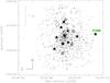 |
Fig. 1 Spatial distribution of our ONC targets (filled stars) and the sample of D’Orazi et al. (2009) re-analyzed in this work (empty stars). Dots represent the Hillenbrand (1997) sample with membership probability higher than 90%. The field is centered on the Trapezium cluster and covers an area of about 0.5° × 0.5°. The position of the star at the edge of the main cluster (P1455) is given. |
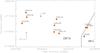 |
Fig. 2 Spatial distribution of our OB1b stars (dots). The field covers an area of ~3° × 1°. The position of ϵ Ori (one of the Orion Belt stars) is also shown. The solid line outlines the boundary between Orion OB1a and OB1b (Warren & Hesser 1977). |
The most recent determination of [Fe/H] in Orion based on late-type stars was performed by D’Orazi et al. (2009), who analyzed a small sample of cool ONC members and one candidate member of the OB1b association. They inferred a solar metallicity for the ONC with a very small star-to-star dispersion ([Fe/H] = −0.01 ± 0.04), along with hints of a slightly sub-solar metallicity for OB1b. While this result might provide support to the sequential star formation scenario, D’Orazi et al. (2009) emphasized that their results should be confirmed based on a larger sample of stars and the analysis of spectra more suitable for abundance measurements.
Here, we present a new study of the elemental abundances in Orion, based on high-resolution spectra obtained with flames/uves on the very large telescope (VLT). Not only is our sample larger than that of D’Orazi et al. (2009), but the spectral range covered by our spectra includes a significantly larger number of Fe i and Fe ii lines, which enabled us to achieve a more secure determination of stellar parameters. Furthermore, for the coolest stars in the sample, the analysis was performed using GAIA models (Hauschildt et al. 1999; Brott & Hauschildt 2010, priv. comm.), which are more appropriate than ATLAS models (Kurucz 1993), because of the inclusion of millions of molecular lines in the line list, as explained in detail in Appendix B. Finally, the sample of D’Orazi et al. (2009) was reanalyzed.
In Sect. 2, we describe the sample, observations, and data reduction. The measurements of radial velocity, effective temperature, veiling, and elemental abundance are given in Sects. 3 and 4. The results, discussion, and conclusions are presented in Sects. 5–7. In Appendix A, we give the line list, while in Appendix B we describe the impact of model atmospheres on abundance measurements.
2. Sample, observations, and data reduction
2.1. The sample
The ONC target stars were taken from Hillenbrand (1997); we selected stars with spectral types from late-G to early-M without evidence of strong accretion and, thus, spectral veiling. We avoided stars with large rotational velocities (vsini > 30 km s-1) and known to be binaries. The total sample contains 10 stars. Similar criteria were applied to the OB1b group, where we selected 10 late-K stars from the Briceño et al. (2005, 2007) samples.
The ONC and OB1b samples are listed in Table 1, along with information from the literature. For the ONC, we indicate in Cols. 1–7 the star name, I magnitude, V − I color, spectral type, effective temperature, luminosity, and membership probability from Hillenbrand (1997) and Hillenbrand et al. (1998), and in Cols. 8–9 the values of vsini (Wolff et al. 2004; Sicilia-Aguilar et al. 2005; Santos et al. 2008) and some notes. For OB1b, we list the star name, V magnitude, V − I color, spectral type, effective temperature from spectral-type using the Kenyon & Hartmann (1995) scale, luminosity, and object class taken from Briceño et al. (2005). In the last two columns of the table, we report our radial velocity measurements and comments on membership (see Sect. 3).
In Figs. 1 and 2, we show the distribution in the sky of our targets. The ONC stars fall inside the main cluster, with the exception of P1455. The case of this star is discussed in Sect. 6.3. As for the OB1b targets, three of them fall close to the OB1b/OB1a boundary defined by Warren & Hesser (1977) and is discussed in Sect. 3.1.
2.2. Observations and data reduction
The observations were obtained in 2009 with the Fiber Large Array Multi-Element Spectrograph (flames; Pasquini et al. 2002) attached to the Kueyen Telescope (UT2) at Paranal Observatory. Both the ONC and OB1b were observed using the fiber link to uves. We allocated fibers to a maximum of seven stars, leaving at least one fiber for the sky acquisition. We used the CD#3 cross-disperser covering the range 4770–6820 Å at the resolution R = 47 000. This setup allowed us to select around 60+9 Fe i+Fe ii lines, as well as spectral features of α- and Fe-peak elements (see Sect. 4.2).
The ONC was covered with two different pointings, each including seven stars with an overlap of four stars. For each pointings, we obtained three 45 min long exposures, resulting in a total integration time of 2 h and 15 min. Three pointings were instead necessary to observe the OB1b stars. The pointings included four, three, and three stars. Each field was observed six, two, and four times, for a total exposure time of 4.5, 1.5, and 3 h. The log book of the observations is given in Table 2.
Data reduction was performed using the flames/uves pipeline (Modigliani et al. 2004) and the following procedure: subtraction of a master bias, order definition, extraction of thorium-argon spectra, normalization of a master flat-field, extraction of the science frame, wavelength calibration of the science frame, and correction of the science frame for the normalized master flat-field. Sky subtraction was performed with the task sarith in the IRAF1echelle package using the fibers allocated to the sky.
All the acquired spectra for each star were shifted in wavelength for the heliocentric correction and then coadded, after checking for possible radial velocity variations. The final signal-to-noise ratio (S/N) is in the range 40–200 for the ONC stars and 30–80 for the fainter OB1b targets. The coadded spectra of the stars we used for abundance measurements are shown in Figs. 3 and 4.
Log of the observations.
3. Radial velocities and membership
Since we did not acquire spectra of radial velocity (RV) standards, we first selected two stars to be used as templates in the ONC and OB1b: JW601 (ONC) and CVSO118 (OB1b). Both have high S/N spectra (~50–100), low vsini (<15 km s-1), and radial velocity measurements from the literature. In particular, CVSO118 is the only star in our OB1b sample with a previous determination of RV. We then measured the RV from the first spectrum we acquired for both stars using the IRAF task rvidlines inside the rv package. This task measures RVs from a line list and we used 25 lines in the spectral range 5800–6800 Å. For JW601, we obtain Vrad = 22.8 ± 0.5 km s-1, while for CVSO118 we find that Vrad = 32.1 ± 0.4 km s-1. These values are in very good agreement with previous determinations of 22.0 ± 0.4 km s-1 and 31.6 ± 0.6 km s-1 obtained by Sicilia-Aguilar et al. (2005) and Briceño et al. (2007), respectively.
Considering JW601 and CVSO118 as templates, we measured the heliocentric RV of all the ONC/OB1b stars using the task fxcor of the IRAF package rv. To take advantage of the wide spectral coverage offered by flames/uves, we cross-correlated all the spectral range of our targets with the template, excluding the regions contaminated by broad emission lines (e.g., Hα) or by prominent telluric features (e.g., the O2 series at λ ≃ 6275 Å). To determine in the most reliable way the centroids of the cross-correlation function (CCF) peaks, we adopted Gaussian fits. The errors in the RV values were computed using a procedure inside the fxcor task that considers the fitted peak height and the antisymmetric noise as described by Tonry & Davis (1979). Since we acquired several spectra per stars, we computed an average RV value for all our targets that did not display evidence of binarity. The average RV values for most probably single stars are listed in Table 1.
3.1. Membership
To confirm the membership of our stars, the distributions of average RV measurements for the ONC are shown in Fig. 5, along with the value derived by Biazzo et al. (2009) for ~100 very low-mass members. Seven out of 10 stars of ONC are confirmed as members and most probably single stars with a mean RV of 24.9 ± 2.6 km s-1 in good agreement with previous determinations (Sicilia-Aguilar et al. 2005; Biazzo et al. 2009). The three exceptions are JW373, JW365, and JW641, which exhibit a double/triple-peaked CCF. We, thus, classify these stars as, previously unidentified, binaries. Two of them (JW365 and JW641) also have a double-lined system (SB2) and are therefore discarded from further analysis.
For OBab, similarly, we compare our sample with the distribution found by Briceño et al. (2007) based on 30 OB1b targets from which they derived a mean RV of 30.1 ± 1.9 km s-1. Five sample stars are confirmed single members, with an average RV of 29.9 ± 3.0 km s-1, while three are non-members and two (CVSO129 and CVSO128) have double/triple-peaked CCFs. Among the non-members, CVSO56 and CVSO58 have RVs close to the OB1a/25 Ori region (mean RV ~20 km s-1; Briceño et al. 2005), as also implied by their spatial location close to the OB1b/OB1a boundary (Fig. 2).
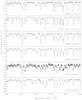 |
Fig. 3 Portion of spectra in the 6220–6270 Å wavelength range of the ONC stars for which we measured the abundances. Different features used for temperature determination using line-depth ratios and abundance measurements are indicated. |
4. Abundance analysis
To summarize, abundances were obtained for all the ONC and OB1b single members or single-lined binaries, with the exception of rapid rotators (JW907, CVSO128, CVSO129, and CVSO161) and the very cool star JW733 for which measuring abundances from line equivalent widths (EW) is not suitable. Since CVSO56 seems to belong to the OB1a/25 Ori subgroup, we measured its iron abundance to gauge the properties of this region. On the other hand, we have not been able to derive the metallicity of CVSO58 because of its rapid rotation.
The analysis was performed using the 2002 version of MOOG (Sneden 1973) that assumes local thermodynamic equilibrium (LTE) and where the radiative and Stark broadening are treated in a standard way. For collisional broadening, we used the Unsöld (1955) approximation. Both Kurucz (1993) and Brott & Hauschildt (2010, priv. comm.) grids of plane-parallel model atmospheres were used for stars warmer and cooler than ~4400 K, respectively (see Appendix B). This is the major change introduced by ourselves with respect to the study of D’Orazi et al. (2009).
4.1. Spectral veiling
We estimated the amount of veiling that affects the spectra of our stars following the procedure described by D’Orazi et al. (2009). In particular, we selected the nine lines in their list included in our spectral range. We then compared the equivalent widths of these lines to those measured in the spectra of 16 members of the open clusters IC 2602 and IC 2391, which are old enough (30-50 Myr; Randich et al. 2001) to ensure that their spectra are not affected by veiling. These IC stars have effective temperatures similar to the ONC/OB1b targets (~4300–5800 K) and their spectra have a resolution close to ours. For each line, we checked whether any dependence of the EW on effective temperature was present; since for most lines we found a weak trend within an interval of 1000 K, we decided to bin the whole temperature range in 500 K steps and derive the mean EWs of the IC stars inside each bin. For two lines, namely Ca i 6102.7 Å and Ca i 6122.2 Å, we found significant trends at all temperatures, hence we used the EW value of the IC cluster star with temperature closer to that of our ONC/OB1b star. For each line, we then obtained the veiling as 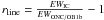 . The mean veiling ⟨ r ⟩ was then computed as the average of all rline values.
By applying this method, we determined a veiling value consistent with zero for all the stars, with the exception of JW373 (r = 0.128 ± 0.080) in the ONC, which is indeed classified as CTTS (Table 1). We thus corrected the measured EWs of all the lines using the relationship between the true EW and the measured one: EWtrue = EWmeas(1 + ⟨ r ⟩ ).
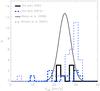 |
Fig. 5 Radial velocity distribution for the most probable single stars in the ONC (solid lines) and OB1b (dashed lines) samples. The thick solid and dashed lines refer to this work. The thin solid line represents the Gaussian fit to the Biazzo et al. (2009) sample obtained for 96 ONC targets with a mean Vrad = 24.87 km s-1 ( |

4.2. Line list, solar analysis, and EWs
We adopted the line list of Randich et al. (2006) integrated with lines from the list of D’Orazi & Randich (2009) included in our wavelength range. We refer to both papers for details on atomic parameters and their sources. The line list is given in Table A.1.
As usually done, our analysis was performed differentially with respect to the Sun. We analyzed the Randich et al. (2006) solar spectrum obtained with uves, using our combined line list and their solar parameters (Teff = 5770 K, log g = 4.44, ξ = 1.1 km s-1). We obtained log n(Fe) = 7.52 ± 0.02 for Kurucz (1993) models and log n(Fe) = 7.51 ± 0.02 for Brott & Hauschildt (2010, priv. comm.) models. The results for all the elements are given in Table 3 together with those given by Anders & Grevesse (1989) and Asplund et al. (2009). We caveat that the latter values were obtained using 3D models. Table 3 shows good agreement between the two model atmospheres and between our and literature values.
The EWs of the target stars were measured by means of a direct integration or Gaussian fitting procedure using the IRAF splot task. Very strong lines (EW ≳ 150 mÅ), which are most affected by the treatment of damping, were excluded from the list; furthermore, a 2-σ clipping was applied to the Fe i list before determining stellar parameters and iron abundance. The abundance of the other elements was derived using the same criteria.
Comparison between solar abundances derived using Kurucz (1993) and Brott & Hauschildt (2010, priv. comm.) model atmospheres.
4.3. Stellar parameters
4.3.1. Effective temperatures
Photometric temperatures were taken from Hillenbrand (1997) for the ONC ( in Table 1), while for the OB1b sample we converted the spectral-types of Briceño et al. (2005) to temperatures using the scale of Kenyon & Hartmann (1995) (
 in Table 1).
Spectroscopic temperatures were then derived in two different ways. It has been demonstrated that line-depth ratios (LDRs) are powerful tools for measuring the effective temperature with a precision as small as 10–50 K for spectra with S/N > 100 (Gray & Johanson 1991; Kovtyukh et al. 2006; Biazzo et al. 2007, and references therein). The precision of this method can be improved by averaging the results from several line pairs. To develop appropriate Teff-LDR calibrations, we considered the synthetic stellar library described and made available by Coelho et al. (2005). These spectra are sampled at 0.02 Å, range from the near-ultraviolet (300 nm) to the near-infrared (1.8 μm), and cover the following grid of parameters: 3500 ≤ Teff ≤ 7000 K, 0.0 ≤ log g ≤ 5.0, −2.5 ≤ [Fe/H] ≤ + 0.5, α-enhancement [α/Fe] = 0.0, 0.4 and microturbulent velocity ξ = 1.0, 1.8, 2.5 km s-1.
Following the prescriptions given by Biazzo et al. (2007), we used their line list in the 6190–6280 Å spectral range and their line pairs, namely 15 (see their Tables 1 and 2; we refer to that paper for a detailed explanation and justification of the line list and line pairs selected). We then measured their LDRs according to the guidelines of Catalano et al. (2002), and developed Teff-LDR calibrations after degrading the synthetic spectra to our resolution. The calibrations were created for 3.0 ≤ log g ≤ 4.5, 4000 ≤ Teff ≤ 6500 K, and vsini = 0 km s-1, considering the synthetic spectra at [Fe/H] = 0.0, [α/Fe] = 0.0, and ξ = 1.0 km s-1.
In the end, the effective temperatures obtained from all the useful LDRs for each ONC/OB1b target were averaged to increase the precision of the temperature determination. The values ( ) are listed in Table 4 and plotted in Figs. 6 and 7.
Astrophysical parameters and chemical abundances derived from our analysis.
As commonly done, effective temperatures were also determined by imposing the condition that the Fe i abundance does not depend on the excitation potential of the lines. These temperatures are defined  (Table 4) and represent the adopted values for the abundance analysis (Sect. 5).
We first note that the two values and closely agree (see Figs. 6 and 7), with the only exception of JW373, which is, as mentioned, a probable binary affected by veiling that has a rather low S/N spectrum. Moreover, in Fig. 6 the agreement of both spectroscopic temperatures with is also good, with the exception of JW868 and JW589, which we find cooler than the Hillenbrand (1997) values on average by ~550 K. For JW733, we can give only an upper limit because Teff-LDR calibrations are suitable for temperatures higher than 4000 K. In Fig. 7, the agreement with is also good within the errors.
4.3.2. Microturbulence velocities and surface gravities
The microturbulence velocity ξ was determined by imposing that the Fe i abundance is independent on the line equivalent widths. The initial microturbulence velocity was set to 1.5 km s-1. The values of ξ are listed in Table 4. We note that our determinations are typically higher than those of D’Orazi et al. (2009). We comment on this in Sect. 5.3.
At variance with D’Orazi et al. (2009), who did not have enough Fe ii features in their spectral range, we were able to estimate the surface gravity log g by imposing the Fe i/Fe ii ionization equilibrium (log gS in Table 4) for all the ONC stars with the exception of JW868, where no Fe ii line was found. For the stars in the ONC, the initial log g was obtained from the relation between mass, luminosity, and temperature (log g = 4.44 + log M + 4log (Teff/5770) − log L, labeled as log gP in Table 4) taking as astrophysical parameters the values given by Hillenbrand (1997). We verified that the effect on the gravity of considering instead of the Hillenbrand (1997) temperature is negligible for our accuracy. We note that the agreement between log gS and log gP is quite good, the difference being at most 0.30 dex.
On the other hand, since the stars in OB1b are cooler than those in the ONC, we did not find any Fe ii lines, with the only exception of a couple of lines in CVSO118 and CVSO125. Thus, we decided to fix the surface gravity to the values obtained using the relation between M, L, and Teff, where the astrophysical parameters were taken from Briceño et al. (2005).
Finally, we remeasured [Fe/H] for the D’Orazi et al. (2009) stars applying the same method used here. We measured the line EWs and derived the atmospheric parameters and iron abundances using ATLAS and GAIA models for stars with effective temperatures higher and lower than 4400 K, respectively.
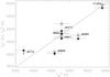 |
Fig. 6 Spectroscopic effective temperatures versus the photometric values obtained by Hillenbrand (1997). Our |
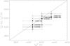 |
Fig. 7 Our spectroscopic effective temperatures versus the values obtained by converting the spectral types given by Briceño et al. (2005) into temperature using the tables of Kenyon & Hartmann (1995). Our |
Our reanalysis of the D’Orazi et al. (2009) sample (left) and D’Orazi et al. (2009) outputs (right).
4.4. Errors
Derived abundances are affected by random (internal) and systematic (external) errors.
Sources of internal errors include uncertainties in atomic and stellar parameters, measured equivalent widths, and the veiling determination.
Uncertainties in atomic parameters, such as the transition probability (log gf), should cancel out, since our analysis is carried out differentially with respect to the Sun.
Errors due to uncertainties in stellar parameters (Teff, ξ, log g) were estimated first by assessing errors in stellar parameters themselves and then by varying each parameter separately, while keeping the other two unchanged. We found that variations in Teff larger than 60 K would introduce spurious trends in log n(Fe) versus the excitation potential (χ), while variations in ξ larger than 0.2 km s-1 would result in significant trends of log n(Fe) versus EW, and variations in log g larger than 0.2 dex would lead to differences between log n(Fe i) and log n(Fe ii) larger than 0.05 dex. The above values were thus assumed as uncertainties in stellar parameters. Errors in abundances (both [Fe/H] and [X/H]) due to uncertainties in stellar parameters are summarized in Table 6 for one of the coolest and the warmest stars in our ONC/OB1b samples.
As for the errors due to uncertainties in EWs, our spectra are characterized by different S/N ratios and it is not possible a priori to estimate a typical error in EW. However, random errors in EW are well represented by the standard deviation around the mean abundance determined from all the lines. These errors are listed in Table 4, where uncertainties in [X/Fe] were obtained by quadratically adding the [Fe/H] error and the [X/H] error. When only one line was measured, the error in [X/H] is the standard deviation of three independent EW measurements. The number of lines employed for the abundance analysis is listed in Table 4 in parentheses, with the exception of those elements (sodium, aluminium, and ionized titanium) where only one or two lines were used.
Finally, as described in Sect. 4.1, the veiling of all the sample stars is negligible, with the only exception of JW373. For this star, we estimate that the veiling contribution to the abundance error is on the order of 0.05–0.11 dex, depending on the element.
The greatest contribution to the external or systematic errors originates in the abundance scale, which is mainly affected by the choice of the model atmospheres. This error source is discussed in Appendix B. Here, we emphasize that we used for both the Orion subgroups the same procedure, instrument set-up, and prescriptions to derive the abundances. As a consequence, differences in abundance between ONC and OB1b should not be influenced by systematic errors linked to the abundance scale.
Internal errors in abundance determination due to uncertainties in stellar parameters for one of the coolest star (namely, CVSO118) and for the warmest star (namely, P1455) in our samples.
5. Results
5.1. Metallicity
Our final abundances are listed in Table 4. The comparison between the new and the D’Orazi et al. (2009) iron abundances is given in Table 5 and shown in Fig. 8. We comment on any differences in Sect. 5.3. In Figs. 9–11, we present [Fe/H], [X/H], and [X/Fe] as a function of Teff for the ONC and OB1b samples. Figure 9 includes both our targets and those from D’Orazi et al. (2009).
Figure 9 shows that, with the only exception of P1455 in the ONC, we do not find a major star-to-star difference in [Fe/H], with a remarkable agreement between the iron abundance of the present sample and that of D’Orazi et al. Excluding the D’Orazi et al. sample, the mean ONC [Fe/H] is −0.15 ± 0.01 (without P1455) and −0.11 ± 0.11 (with P1455). Including those stars, we find similar values, namely −0.13 ± 0.03 and −0.11 ± 0.08, respectively. As for OB1b, the star-to-star difference is minimal, considering the rather large uncertainty that affects the measurement of the coolest star. The mean for OB1b is [Fe/H] = −0.05 ± 0.05, i.e. almost 0.1 dex above the ONC, although marginally consistent with it.
Moreover, Fig. 9 does not reveal any trend between [Fe/H] and effective temperature, with the exception again of P1455, the warmest star of the sample. Therefore, we believe that the difference between the [Fe/H] values of the ONC and OB1b is not due to systematic effects related to the effective temperature.
Finally, we mention that for the likely OB1a/25 Ori member (CVSO56) we find [Fe/H]=−0.08 ± 0.15, a value very close to that of the ONC and OB1b (see Fig. 9).
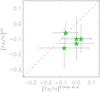 |
Fig. 8 Our iron abundance measurements of the D’Orazi et al. (2009) sample versus their outputs. |
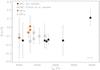 |
Fig. 9 [Fe/H] versus |
5.1.1. [Fe/H] difference between ONC and OB1b?
As mentioned in the Introduction, D’Orazi et al. (2009) found that the only star of OB1b (HD294297) was ~0.1 dex more metal-poor than the ONC. Caballero (2010) demonstrated that it is a non-member of the association. Our new results show that the average [Fe/H] of OB1b is slightly higher than that of ONC. The question then arises of whether the ONC is intrinsically more metal-poor than OB1b or there are systematic effects in the analysis.
We note that NLTE effects have indeed been found to be important for cool stars with relatively high gravity, leading to an overestimate of the [Fe/H] (Takeda 2008; Schuler et al. 2010). In Fig. 12, we show [Fe/H] versus log g for our ONC/OB1b stars cooler than 4500 K; the figure shows a moderate increase in the abundance with log g > 4.0. Although we cannot quantitatively estimate the amount of NLTE effects, we suggest that they might account for the difference between the ONC and OB1b metallicities.
5.2. Other elements
In Figs. 10 and 11, we plot [X/H] and [X/Fe] as a function of Teff for the different elements derived in this study. These figures show that no trends are present for silicon and nickel, with the only exception of P1455, which is a “rich” star in terms of all elements, included iron (see Sect. 6.3). Its values of [X/Fe] are instead close to the solar ones (Fig. 11). In contrast, Na, Al, Ca, and Ti i are lower for stars cooler than ~4500 K both when considering [X/H] and when considering [X/Fe].
Similar results have been found by several authors (e.g., Schuler et al. 2003, 2006; Yong et al. 2004; Beirão et al. 2005; Gilli et al. 2006; D’Orazi & Randich 2009) and ascribed to NLTE effects. In particular, D’Orazi & Randich (2009) in their analysis of the young clusters IC 2602 and IC 2391 show that, while the [Ti i/Fe] ratio decreases with decreasing temperature, [Ti ii/Fe] increases, suggesting that over-ionization is at work. Owing to their young age, cluster stars are characterized by enhanced levels of chromospheric activity and are more affected by NLTE over-ionization. As suggested by the aforementioned authors, deviations from LTE are possibly responsible for the effects seen in Fig. 11 for Na, Al, Ca, and Ti elements. On the other hand, Ni and Si lines have higher ionization potentials (7.63 and 8.15 eV, respectively) than Na, Al, Ca, and Ti (~5.14−6.82 eV) and are thus less affected by over-ionization.
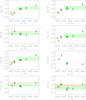 |
Fig. 10 [X/H] versus |

Regardless of the physical reasons for the observed behavior, we computed the mean [X/Fe] ratios for sodium, aluminum, and calcium considering only the ONC/OB1b stars with temperatures higher than 4500 K (Table 4). In the case of titanium, where some ionized lines were measured, we list the average coming from Ti i and Ti ii. There is no significant difference in the average values between the two subgroups and the dispersion observed in the elemental abundances of each subgroup is smaller than the observational uncertainties. The average [X/Fe] values are close to solar, with Na, Al, and Si being slightly overabundant.
5.3. Comparison with results of other authors
Some of our sample stars have been observed by other authors. In particular, one star, JW157 = KM Ori, is in common with the Padgett (1996) sample. She finds for this star [Fe/H] = + 0.14 ± 0.18, which disagrees significantly with our iron abundance (Δ[Fe/H] = 0.29 dex). Possible explanations include:
-
i)
The Padgett abundance analysis was based on fewer iron lines(17) than our own (40 lines; see Table 4);
-
ii)
whereas we excluded very strong lines with EW > 150 mÅ (see Sect. 4.2), 6 among 17 lines in the Padgett list have EW > 150 mÅ (see her Table 9);
-
iii)
seven lines of the Padgett list are in common with us, but for four of those we find different EWs of about ± 15–20 mÅ. We carefully re-measured these lines confirming our original values. We conclude that our determination is likely to be more reliable.
Both the mean [Fe/H] value for the ONC and [X/Fe] ratios found by ourselves are in good agreement with the results of Santos et al. (2008), who derived a mean metallicity of [Fe/H] = −0.13 ± 0.06 and Ni and Si abundances [Ni/Fe] = −0.06 ± 0.07 and [Si/Fe] = 0.00 ± 0.09, respectively. In particular, two of three stars of their sample (JW589 and JW157) are in common with ours. There is a reasonable agreement between the abundances for these two stars, and any differences can be accounted for by the different line lists and σ-clipping criteria used.
As shown in Sect. 4.3, the present results yield a lower [Fe/H] than D’Orazi et al. (2009). The main reasons for this discrepancy are:
-
i)
our new analysis is based on more suitable spectra and line list ofFe i, which allow us to more tighly constrain theabundance versus χ and versus EW trends, hence the Teff and ξ values;
-
ii)
our analysis of stars with Teff ≲ 4400 K is based on GAIA atmospheric models that are more appropriate for cool stars (as discussed in Appendix B);
-
iii)
critical and careful reanalysis of the CD#4 spectra acquired by D’Orazi et al. allowed us to derive the microturbulence value of the star # 673, which had been not inferred by these authors.
6. Discussion
6.1. Triggered star formation and chemical self-enrichment
Orion is regarded as a proto-type of triggered star formation, where star formation has proceeded sequentially (Preibisch & Zinnecker 2006). As mentioned in the Introduction, this scenario predicts a peculiar chemical enrichment due to contamination of material ejected from type-II supernovae (SNIIe) originating from a first generation of massive stars, since these are expected to contain the nucleosynthetic products of the stellar interior.
In support of this view, Cunha & Lambert (1992, 1994) found that stars in the young subgroup 1d and some of the slightly older subgroup 1c have an abundance up to about 40% higher than the rest of their sample. They suggested that the enrichment resulted from the mixing of SNIIe ejecta from the 1c subgroup to the center of the Trapezium cluster. Simón-Díaz (2010) derived homogeneous values of the oxygen and silicon abundances in stars of the four subgroups (OB1a,b,c,d), which had a dispersion (~0.04 dex) smaller than the intrinsic uncertainties (~± 0.10 dex).
Our results indicate that low-mass stars yield the same abundance distribution as high-mass stars (see Simón-Díaz 2010). In particular, Si is the only α-element that does not exhibit strong evidence of being affected by NLTE on the basis of our data (see Fig. 11) and for which we obtained abundances for both ONC-OB1d and OB1b. We find group-to-group dispersions of ~0.08 and ~0.01 dex in [Si/H] and [Si/Fe], respectively, which are smaller than our internal errors (of around ± 0.11–0.31 and ± 0.13–0.36 dex, respectively). The other elements for which we measured the abundance is titanium. We find for this element a difference of 0.08 dex for ⟨ [Ti/H] ⟩ and 0.01 dex for ⟨ [Ti/Fe] ⟩ ; this is smaller than our internal errors (around ±0.10–0.15 and ±0.12–0.31 dex, respectively).
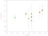 |
Fig. 12 [Fe/H] versus log g for the coolest stars (Teff < 4500 K) of our and D’Orazi et al. re-analyzed samples (stars: ONC; circles: OB1b). |
We conclude that the ONC and OB1b are characterized by homogeneous silicon and titanium abundances. This means that even if SNII explosions occurred in OB1b, at the OB1b-ONC distance their ejecta did not have the conditions to chemically enrich the ONC stars, dispersing the element over a large volume.
As for the difference in [Fe/H] between the ONC and OB1b (should it be real), we note that an inhomogeneity in metallicity (at the level of ~0.05 dex) within a given star-forming complex is expected in models of hierarchical star formation (Elmegreen 1998). Owing their chaotic and large-scale formation process on a 1 kpc scale, the gas in a giant molecular cloud will have a range of metallicities reflecting the background Galactic gradient. We find this unlikely because the separation between ONC and OB1b (<50 pc) is much smaller than the scale on which the Galactic gradient operates.
6.2. The metallicity of SFRs: comparison with young open clusters
Our present analysis reinforces the conclusion of Santos et al. (2008) that none of the SFRs with available metallicity is more metal-rich than the Sun; the majority of them are indeed slightly more metal-poor. Santos et al. (2008) suggest that, if the lower-than-solar metallicities of SFRs were confirmed, this would imply that either the Sun was formed in an inner region of the Milky Way disk, or that the nearby interstellar medium experienced a recent infall of metal-poor gas.
D’Orazi & Randich (2009) demonstrated that the abundance pattern of young open clusters in the solar neighborhood is identical to the solar distribution, concluding that the Sun was most likely born at the present location. In Fig. 13, we compare the distribution of [Fe/H] of the SFRs within 500 pc of the Sun with that of i) open clusters younger than ~150 Myr within the same distance from the Sun; and ii) young nearby loose associations. In addition to the [Fe/H] values for the ONC and OB1b derived here, metallicity determinations for other SFRs were retrieved from Santos et al. (2008 – Chamaeleon, ρ Ophiucus, Corona Australis, Lupus), Gonzàlez-Hernàndez et al. (2008 – σ Orionis), and D’Orazi et al. (in prep. – Taurus). [Fe/H] values for the young associations were taken from Viana Almeida et al. (2009 – their “uncorrected” values were considered).
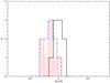 |
Fig. 13 [Fe/H] distribution for: SFRs within 500 pc from the Sun (dashed histogram), young nearby loose associations (dot-dashed line), and open clusters younger than 150 Myr and within 500 pc from the Sun (solid line). Sources of [Fe/H] values for the young open clusters are the following: α Persei (Boesgaard & Friel 1990), NGC 2516 (Terndrup et al. 2002), NGC 2451A/B (Hünsch et al. 2004), Blanco 1 (Ford et al. 2005), IC 4665 (Shen et al. 2005), IC 2602 and IC 2391 (D’Orazi & Randich 2009), and Pleiades (Soderblom et al. 2009). |
The figure shows that the three distributions, in particular that of open clusters, are characterized by a small dispersion; however, the cluster distribution is shifted towards somewhat higher metallicities than the SFRs and young associations. We obtain average values of [Fe/H] = −0.06 ± 0.04,−0.06 ± 0.04, and −0.01 ± 0.03 for the SFRs, associations, and open clusters, respectively. In addition, none of the open clusters is as metal-poor as the most metal-poor SFR (the ONC) and only three out of nine SFRs fall within the open cluster distribution. In other words, not only the SFRs are more metal-poor than the Sun, but they are on average more metal-poor than young open clusters, which should be representative of the metallicity in the solar neighborhood. As for the loose associations, their distribution is in closer agreement with that of the SFRs than with the clusters; we note, however, that the “corrected” values of Viana Almeida et al. (2009) would yield a higher metallicity. Higher values of [Fe/H] were also derived by Rojas et al. (2008) for a sample of Tucana-Horologium members.
Focusing on the comparison between clusters and SFRs, the offset between their mean [Fe/H] values is small and still based on relatively small number statistics. One might have missed the more metal-rich SFRs or, viceversa, the more metal-poor open clusters in the solar vicinity. In addition, whereas an agreement on the metallicity of the ONC seems now to have been reached, discrepancies still exist for other regions; for example, Santos et al. (2008) find [Fe/H] = −0.08 ± 0.12 for Ophiucus, compared to the value [Fe/H] = 0.08 ± 0.07 derived by Padgett (1996). This indicates that additional homogeneous studies must be performed, before the conclusion that SFRs are slightly more metal-poor than the Sun and the open clusters can be definitively drawn.
With this caveat in mind, we would like to point out that, given the young age of the clusters, stellar migration is unlikely to be the reason for the difference in the [Fe/H] distributions of the open clusters and SFRs. The difference likely reflects a difference in the interstellar gas from which members of SFRs and young clusters formed. This in turn must be a relic of the process of star formation in the solar neighborhood, rather than an effect of chemical evolution, given the short timescales involved, and that in any case chemical evolution would lead to the younger regions (i.e., the SFRs) being more metal-rich than the older clusters.
6.3. The case of P1455: a metal-rich star?
P1455 is significantly more metal-rich than the ONC stars. For this target, we derived an iron abundance of 0.11 ± 0.09 in very good agreement with the Cunha et al. (1995) value of [Fe/H] = 0.08 ± 0.15, which confirms that this star is more metal-rich than the other ONC targets at the 2-σ level. Although this is still marginally consistent with what is expected from statistical fluctuations, some discussion of this object would be merited.
At present, we do not have reasons to consider this star as a non-member of the ONC. Its radial velocity and proper motion are consistent with membership. We also note that we obtained an independent RV estimate using spectra acquired with harps (High Accuracy Radial velocity Planet Searcher; Mayor et al. 2003), yielding a mean Vrad of 21.893 ± 0.014 km s-1.
As noted in Sect. 2, this star is farther away from the main cluster than the other targets. Its higher metallicity may imply that the ONC region is inhomogeneous on scales of 1–2 pc and that one could search for other metal-rich stars close to P1455.
We recall that whether super-solar metallicity stars exists in SFRs has been disputed for a few years (Santos et al. 2008, and references therein), and is relevant because circumstellar disks around young stars are the birthplace of planets. Thus, “P1455-like cases” in SFRs may well be good targets for exoplanet searches.
7. Conclusions
We have presented new measurements of the abundances of iron-peak elements and α-elements in two subgroups of the Orion complex, the Orion Nebula Cluster (ONC), and the OB1b sub-association, derived from flames/uves high-resolution spectroscopy. Our main results can be summarized as follows:
-
The ONC and OB1b have mean iron abundances of −0.11 ± 0.08 and −0.05 ± 0.05,respectively. A likely member of OB1a has an abundance of[Fe/H] = −0.08 ± 0.15. We can exclude themetallicity of Orion being above the solar value.
-
The ONC and OB1b are characterized by a small scatter in iron abundances, with the only exception of P1455 in the ONC, which we confirm to be metal-rich, as found in previous studies (Cunha et al. 1998; Cayrel de Strobel et al. 2001).
-
In the temperature range where NLTE effects are less evident (i.e. ≳ 4500 K), there is no presence in the ONC sample of star-to-star inhomogeneity in the abundances of the elements strongly affected by these effects (namely Na, Al, Ca, Ti i). Owing to the lower temperatures of the OB1b sample, we are unable to draw any conclusions about these elements. For elements not strongly affected by NTLE effects (namely, Si and Ni) both the ONC and OB1b do not show any star-to-star abundance inhomogeneity.
-
The two sub-associations analyzed here have similar solar abundances of the α-elements silicon and titanium (the latter obtained by averaging the abundance of Ti i and Ti ii). Similar nickel abundances were found for the two Orion subgroups. No evidence of self-enrichment from OB1b to the ONC is found.
-
Star-forming regions and open clusters younger than 150 Myr and within 500 pc of the Sun were found to have a small offset between their mean iron abundance, with the former being more metal-poor than the latter. Owing to the young age of both sets of stars, this offset probably reflects a difference in the properties of the interstellar gas from which members of SFRs and young clusters formed. More homogeneous studies are required to draw definitive conclusions.
Online material
Appendix A: Line list
Wavelength, elements, excitation potential, and oscillator strength of all the elements are listed.
Appendix B: Elemental abundance analysis of cool stars: dependence on model atmospheres
Many possible fallacies can affect the process going from the spectroscopic stellar observations to the derivation of the chemical composition using atomic parameters and the derivation of stellar parameters. We focus here on the role of model atmospheres. In particular, we show how the use of different model atmospheres leads to different results in metallicity and other elemental abundances (i.e., sodium, aluminum, silicon, calcium, titanium, and nickel).
B.1. The test
In the following, we present our starting points:
-
We considered three young members of ONC and OB1b (namely,CVSO159, CVSO118, and KM Ori) because theycover a wide range in effective temperature (Teff ~ 4000−4700 K)and surface gravity (log g ~ 3.0−4.5), but our discussion can be extended to alllate-G/early-M stars. We also considered, as a comparison, asolar spectrum acquired by Randichet al. (2006) with flames/uves at asimilar resolution of the other spectra.
-
Abundance analysis was carried out following the steps given in Sect. 4.
-
We considered low-resolution (20 Å) ATLAS2 (Kurucz 1993) and high-resolution (2 Å) GAIA3 (Hauschildt et al. 1999; Brott & Hauschildt 2010, priv. comm.) synthetic spectra to evaluate the continuum flux around lines and in photometric bands normally used for line EW measurements (see Sect. B.2). ATLAS spectra cover the ultraviolet (1000 Å) to infrared (10 μm) spectral range, while GAIA spectra cover the 300 Å ≲ λ ≲ 100 μm wavelength range.
-
Kurucz (1993) and Brott & Hauschildt (2010, priv. comm.) grids of plane parallel model atmospheres were considered for the abundance measurements (see Sect. B.3). ATLAS includes atmosphere models with metallicities −5.0 ≤ [Fe/H] ≤ + 1.0, gravity range 0.0 ≤ log g ≤ 5.0, and 3500 ≤ Teff ≤ 10 000 K. GAIA model atmospheres span in 2000 ≤ Teff ≤ 10 000 K, 0.0 ≤ log g ≤ 5.5, and −4.0 ≤ [Fe/H] ≤ + 0.5. Model atmospheres for specific stellar parameters of our interest were generated by interpolating in the original ATLAS and GAIA grids (see the procedure described by Bean et al. 2006).
B.2. Implications on continuum flux
One of the most important improvements made to the GAIA models was the inclusion of millions of molecular lines in the line list. This is of paramount importance when computing the band opacity, in addition to the line opacity. The effects of band opacities on the continuum flux are most pronounced in the optical domain that is largely used for abundance measurements (namely, 4000–8000 Å).
To help identify the range in effective temperature where the two grids of models can be used for abundance measurements, we calculated the GAIA average continuum fluxes in 20 Å windows centered on λ4900, 5600, 6300, and 7500 Å, which are typical regions used for abundance determinations. These fluxes were evaluated for solar-scaled chemical composition. Continuum flux at the same wavelengths were also considered for ATLAS low-resolution spectra (sampled at 20 Å) of solar abundance. The comparison of these fluxes is shown in Fig. B.1, for log g = 4.0 and for 3000 ≤ Teff ≤ 7500 K, which are a typical gravity and temperatures of low-mass members of star-forming regions. At all temperatures, the flux obtained with the GAIA model is lower than the flux obtained using ATLAS models, but for Teff ≲ 4400 K (depending on the line wavelength) the flux decrement of GAIA spectra is more pronounced than the ATLAS spectra. This is particularly evident, for instance, at λ = 5600, 6300 Å, and is due to the formation in stellar spectra of molecular bands, such as metal oxide (most of all TiO, but also VO), hydroxide (such as OH), hybrids (such as CaH, FeH, MgH) in the visible, and CO and H2O in the near infrared. These bands are not accurately reproduced by ATLAS models, which lack line opacity computations for both triatomic molecules (with the exception of H2O) and numerous diatomic molecular transitions (such as VO).
Since the lines used for abundance measurements are spread over wide spectral ranges (typically in the 4000−8000 Å range), we also calculated the synthetic fluxes in the Johnson BVRI-bands by integrating the synthetic ATLAS and GAIA spectra, weighted by the Johnson transmission curve of the BVRI filters. The results are shown in Fig. B.2 for log g = 4.0. The shift between the ATLAS and GAIA models also appears in the BVRI-fluxes, even if it is less evident than the line-continuum fluxes of Fig. B.1, because of the integration over the band wavelengths.
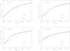 |
Fig. B.1 Comparison between continuum flux at λ4900, 5600, 6300, 7500 Å obtained with ATLAS spectra (squares and dashed line) and GAIA spectra (asterisks and dotted line) at log g = 4.0 as a function of Teff. The lines represent an interpolation through the points. |
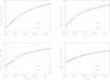 |
Fig. B.2 Comparison between continuum flux at the Johnson BVRI-bands obtained with ATLAS spectra (squares and dashed line) and GAIA spectra (asterisks and dotted line) at log g = 4.0 as a function of Teff. The lines represent an interpolation through the points. |
Examples of Fe, Na, Al, Si, Ca, Ti, and Ni mean abundances obtained for stars in the Orion complex using ATLAS (A) and GAIA (G) models.
B.3. Implications on abundance determination
To search for the effect on abundances, we compared the metallicities and the Na, Al, Si, Ca, Ti, Ni abundances obtained using ATLAS and GAIA models for CVSO159, CVSO118, KM Ori, and the Sun. The results are listed in Table B.1 for both ATLAS and GAIA models.
B.3.1. Iron
The comparison of metallicities is shown in Fig. B.3, where the difference between the two models increases with decreasing temperature, because of the presence of the mentioned bands. In particular, at Teff = 4000−4300 K the difference in abundance is ± 0.07−0.08 dex, while for the Sun the difference is only ± 0.01 dex (see also Table B.1). As a consequence, for a differential abundance analysis with respect to the Sun, for KM Ori (at 4700 K) we do not find almost any difference between the two models, while for both CVSO159 (at 4000 K) and CVSO118 (at 4300 K) the differences are [Fe/H] [Fe/H]
 , + 0.08 dex, respectively. This means that the strong departure of the GAIA model from the ATLAS behavior at ~4400 K shown in Fig. B.1 affects iron abundance, leading to similar differences in stars with
Teff ≲ 4400 K. The lower metallicity resulting from GAIA models (with respect to the ATLAS models) depends on the more signidicant formation of molecules in atmospheres with lower temperatures. The molecular opacity considered in the GAIA models indeed leads to a redistribution of the flux, which is on average lower than the ATLAS one, because of the molecular absorption (line blanketing). Lower flux yields lower intrinsic line equivalent widths, which can be reproduced by lower iron abundances.
B.3.2. Other elements
In Table B.1, we summarize how the use of different models can affect the elemental abundance. Here, the comparison between ATLAS and GAIA grids is listed for Na, Al, Si, Ca, Ti, and Ni. While lines of elements across over the whole spectrum (~4800−6800 Å) infer very different results (such as Ni, besides Fe), elements such as Al, with only two lines at 6696 Å and 6698 Å close each other and not strongly affected by band opacity, lead to similar GAIA and ATLAS abundances.
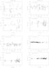 |
Fig. B.3 Comparison of iron abundances derived by using ATLAS and GAIA model atmospheres as a function of equivalent width (EW) and line excitation potential (EP). These examples display the results obtained for stars with four different temperatures. Circles and asterisks refer to abundances derived with ATLAS and GAIA models, respectively, while solid and dashed lines represent their mean values. Vertical thick and thin bars in the log n(Fe) vs. EW panels are the standard deviations around the average iron abundances. |
B.4. Concluding...
We find Teff ≈ 4400 K to be the lower limit where the models in which the line opacity computations are not fully treated, such as ATLAS, can be applied in an abundance analysis. This has been demonstrated for both iron abundance, typically derived by many lines, and other elements (α- and iron-peak elements) typically used as tracers of chemical enrichment.
Acknowledgments
The authors are very grateful to the referee for a careful reading of the paper and constructive suggestions. Jacob Bean provided some IDL codes, for which we are grateful. We thank Daniele Galli, Laura Magrini, and Fabrizio Massi for very useful discussions. This research has made use of the SIMBAD database, operated at CDS (Strasbourg, France), and of the WEBDA database, operated at the Institute for Astronomy of the University of Vienna.
References
- Anders, E., & Grevesse, N. 1989, Geochim. Cosmochim. Acta, 53, 197 [Google Scholar]
- Asplund, M., Grevesse, N., Sauval, A. J., & Scott, P. 2009, ARA&A, 481, 522 [Google Scholar]
- Bally, J. 2008, in Handbook of Star Forming Regions, I, The Northern Sky ASP Monograph Publications, ed. B. Reipurth, 4, 459 [Google Scholar]
- Bean, J., Sneden, C., Hauschildt, P. H., et al. 2006, ApJ, 652, 1604 [NASA ADS] [CrossRef] [Google Scholar]
- Beirão, P., Santos, N. C., Israelian, G., et al. 2005, A&A, 438, 251 [NASA ADS] [CrossRef] [EDP Sciences] [Google Scholar]
- Biazzo, K., Frasca, A., Catalano, S., & Marilli, E. 2007, AN, 328, 938 [NASA ADS] [CrossRef] [Google Scholar]
- Biazzo, K., Melo, C. F. H., Pasquini, L., et al. 2009, A&A, 508, 1301 [NASA ADS] [CrossRef] [EDP Sciences] [Google Scholar]
- Blaauw, A. 1964, ARA&A, 2, 213 [NASA ADS] [CrossRef] [Google Scholar]
- Boesgaard, A. M., & Friel, E. D. 1990, ApJ, 351, 467 [Google Scholar]
- Briceño, C., Calvet, N., Hernández, J., et al. 2005, A&A, 129, 907 [Google Scholar]
- Briceño, C., Hartmann, L., Hernández, J., et al. 2007, A&A, 661, 1119 [Google Scholar]
- Caballero, J. A. 2010, A&A, 514, A18 [NASA ADS] [CrossRef] [EDP Sciences] [Google Scholar]
- Catalano, S., Biazzo, K., Frasca, A., & Marilli, E. 2002, A&A, 394, 1009 [NASA ADS] [CrossRef] [EDP Sciences] [Google Scholar]
- Cayrel de Strobel, S., Soubiran, C., & Ralite, N. 2001, A&A, 373, 159 [NASA ADS] [CrossRef] [EDP Sciences] [Google Scholar]
- Coelho, P., Barcuy, B., Meléndez, J., et al. 2005, A&A, 443, 735 [NASA ADS] [CrossRef] [EDP Sciences] [Google Scholar]
- Cunha, K., & Lambert, D. L. 1992, ApJ, 399, 586 [NASA ADS] [CrossRef] [Google Scholar]
- Cunha, K., & Lambert, D. L. 1994, ApJ, 426, 170 [NASA ADS] [CrossRef] [Google Scholar]
- Cunha, K., Smith, V. V., & Lambert, D. L. 1995, ApJ, 452, 634 [NASA ADS] [CrossRef] [Google Scholar]
- Cunha, K., Smith, V. V., & Lambert, D. L. 1998, ApJ, 493, 195 [NASA ADS] [CrossRef] [Google Scholar]
- Cutri, R. M., Skrutskie M. F., Van Dyk, S., et al. 2003, Explanatory Supplement to the 2MASS All Sky Data Release [Google Scholar]
- D’Orazi, V., & Randich, S. 2009, A&A, 501, 553 [NASA ADS] [CrossRef] [EDP Sciences] [Google Scholar]
- D’Orazi, V., Randich, S., Flaccomio, E., et al. 2009, A&A, 501, 973 [NASA ADS] [CrossRef] [EDP Sciences] [Google Scholar]
- D’Orazi, V., Biazzo, K., & Randich, S. 2010, A&A, accepted [Google Scholar]
- Elmegreen, B. G. 1998, in Abundance Profiles: Diagnostic Tools for Galaxy History, ed. D. Friedli, M. Edmunds, C. Robert, & L. Drissen, ASP Conf. Ser. 147, 278 [Google Scholar]
- Feigelson, E. D., Broos, P., Gaffney, J. A., et al. 2002, ApJ, 574, 258 [NASA ADS] [CrossRef] [Google Scholar]
- Ford, A., Jeffries, R. D., & Smalley, B. 2005, MNRAS, 364, 272 [NASA ADS] [CrossRef] [Google Scholar]
- Gezari, D. Y., Pitts, P. S., & Schmitz, M. 1999, Catalog of Infrared Observations, ed. 5 [Google Scholar]
- Gilli, G., Israelian, G., Ecuvillon, A., et al. 2006, A&A, 449, 723 [NASA ADS] [CrossRef] [EDP Sciences] [Google Scholar]
- González-Hernández, J. I., Caballero, J. A., Rebolo, R., et al. 2008, A&A, 490, 1135 [NASA ADS] [CrossRef] [EDP Sciences] [Google Scholar]
- Gray, D. F., & Johanson, H. L. 1991, PASP, 103, 439 [NASA ADS] [CrossRef] [Google Scholar]
- Hauschildt, P. H., Allard, F., & Baron, E. 1999, ApJ, 512, 377 [NASA ADS] [CrossRef] [Google Scholar]
- Hillenbrand, L. A. 1997, AJ, 113, 1733 [NASA ADS] [CrossRef] [Google Scholar]
- Hillenbrand, L. A., Strom, S. E., Calvet, N., et al. 1998, AJ, 116, 1816 [NASA ADS] [CrossRef] [Google Scholar]
- Hünsch, M., Randich, S., Hempel, M., et al. 2004, A&A, 418, 539 [NASA ADS] [CrossRef] [EDP Sciences] [Google Scholar]
- Johnson, J. A., Aller, K. M., Howard, A. W., & Crepp, J. R. 2010, PASP, 122, 905 [NASA ADS] [CrossRef] [Google Scholar]
- Jones, B. F., & Walker, M. F. 1988, AJ, 95, 1755 [NASA ADS] [CrossRef] [Google Scholar]
- Kenyon, S. J., & Hartmann L. 1995, ApJ, 101, 117 [Google Scholar]
- Kovtyukh, V. V., Soubiran, C., Bienaymé, O., et al. 2006, MNRAS, 371, 879 [NASA ADS] [CrossRef] [Google Scholar]
- Kurucz, R. L. 1993, ATLAS9 Stellar Atmosphere Programs and 2 km s-1 grid, (Kurucz CD-ROM No. 13) [Google Scholar]
- Mayor, M., Pepe, F., Queloz, D., et al. 2003, The Messenger, 114, 20 [NASA ADS] [Google Scholar]
- Modigliani, A., Mulas, G., Porceddu, I., et al. 2004, The Messenger, 118, 8 [NASA ADS] [Google Scholar]
- Padgett, D. L. 1996, ApJ, 471, 847 [NASA ADS] [CrossRef] [Google Scholar]
- Parenago, P. P. 1954, Trudy Gosud. Astron. Sternberga, 25, 1 [NASA ADS] [Google Scholar]
- Pasquini, L., Avila, G., Blecha, A., et al. 2002, The Messenger, 110, 1 [NASA ADS] [Google Scholar]
- Preibisch, T., & Zinnecker, H. 2006, in Triggered Star Formation in a Turbulent ISM, ed. B. G., Elmegreen, & J. Palouš, IAU Symp., 237, 270 [Google Scholar]
- Randich, S., Pallavicini, R., Meola, G., et al. 2001, A&A, 372, 862 [NASA ADS] [CrossRef] [EDP Sciences] [Google Scholar]
- Randich, S., Sestito, P., Primas, F., et al. 2006, A&A, 450, 557 [NASA ADS] [CrossRef] [EDP Sciences] [Google Scholar]
- Rebull, L. M., Stauffer, J. R., Megeath, S. T., et al. 2006, ApJ, 646, 297 [NASA ADS] [CrossRef] [Google Scholar]
- Reeves, H. 1972, A&A, 19, 215 [NASA ADS] [Google Scholar]
- Reeves, H. 1978, in Protostars and Planets, ed. T. Gehrels, IAU Coll., 52, 399 [Google Scholar]
- Rojas, G., Gregorio-Hetem, J., & Hetem, A. Jr. 2008, A&A, 387, 1335 [Google Scholar]
- Santos, N. C., Melo, C., James, D. J., et al. 2008, A&A, 480, 889 [NASA ADS] [CrossRef] [EDP Sciences] [Google Scholar]
- Schuler, S. C., King, J. R., Fischer, D. A., et al. 2003, ApJ, 125, 2085 [Google Scholar]
- Schuler, S. C., Hatzes, A. P., King, J. R., et al. 2006, ApJ, 131, 1057 [CrossRef] [Google Scholar]
- Schuler, S. C., Plunkett, A. L., King, J. R., & Pinsonneault, M. H. 2010, PASP, 122, 766 [NASA ADS] [CrossRef] [Google Scholar]
- Shen, Z.-X., Jones, B., Lin, D. N. C., et al. 2005, ApJ, 635, 608 [NASA ADS] [CrossRef] [Google Scholar]
- Sicilia-Aguilar, A., Hartmann, L. W., Szentgyorgyi, A. H., et al. 2005, AJ, 129, 363 [NASA ADS] [CrossRef] [Google Scholar]
- Simón-Díaz, S. 2010, A&A, 510, 22 [Google Scholar]
- Sneden, C. 1973, ApJ, 184, 839 [NASA ADS] [CrossRef] [Google Scholar]
- Soderblom, D. R., Laskar, T., Valenti, J. A., et al. 2009, AJ, 138, 1292 [NASA ADS] [CrossRef] [Google Scholar]
- Takeda, Y. 2008, in The Metal-Rich Universe, ed. G. Israelian, & G. Meynet (Cambridge: University Press), 308 [Google Scholar]
- Terndrup, D. M., Pinsonneault, M., Jeffries, R. D., et al. 2002, ApJ, 576, 950 [NASA ADS] [CrossRef] [Google Scholar]
- Tonry, J., & Davis, M. 1979, AJ, 84, 1511 [NASA ADS] [CrossRef] [Google Scholar]
- Unsöld, A. 1955, in Physik der Sternatmosphären, (Berlin: Springer-Verlag) [Google Scholar]
- Viana Almeida, P., Santos, N. C., Melo, C., et al. 2009, A&A, 501, 965 [NASA ADS] [CrossRef] [EDP Sciences] [Google Scholar]
- Warren, W. H., & Hesser, J. E. 1977, ApJS, 34, 115 [NASA ADS] [CrossRef] [Google Scholar]
- Wolff, S. C., Strom, S. E., & Hillenbrand, L. A. 2004, ApJ, 601, 979 [NASA ADS] [CrossRef] [Google Scholar]
- Yong, D., Lambert, D. L., Allen de Prieto, C., & Paulson, D. B. 2004, ApJ, 603, 697 [NASA ADS] [CrossRef] [Google Scholar]
All Tables
Comparison between solar abundances derived using Kurucz (1993) and Brott & Hauschildt (2010, priv. comm.) model atmospheres.
Our reanalysis of the D’Orazi et al. (2009) sample (left) and D’Orazi et al. (2009) outputs (right).
Internal errors in abundance determination due to uncertainties in stellar parameters for one of the coolest star (namely, CVSO118) and for the warmest star (namely, P1455) in our samples.
Wavelength, elements, excitation potential, and oscillator strength of all the elements are listed.
Examples of Fe, Na, Al, Si, Ca, Ti, and Ni mean abundances obtained for stars in the Orion complex using ATLAS (A) and GAIA (G) models.
All Figures
|
Fig. 1 Spatial distribution of our ONC targets (filled stars) and the sample of D’Orazi et al. (2009) re-analyzed in this work (empty stars). Dots represent the Hillenbrand (1997) sample with membership probability higher than 90%. The field is centered on the Trapezium cluster and covers an area of about 0.5° × 0.5°. The position of the star at the edge of the main cluster (P1455) is given. |
| In the text | |
|
Fig. 2 Spatial distribution of our OB1b stars (dots). The field covers an area of ~3° × 1°. The position of ϵ Ori (one of the Orion Belt stars) is also shown. The solid line outlines the boundary between Orion OB1a and OB1b (Warren & Hesser 1977). |
| In the text | |
|
Fig. 3 Portion of spectra in the 6220–6270 Å wavelength range of the ONC stars for which we measured the abundances. Different features used for temperature determination using line-depth ratios and abundance measurements are indicated. |
| In the text | |
 |
Fig. 4 As in Fig. 3 but for the OB1b sample. |
| In the text | |
|
Fig. 5 Radial velocity distribution for the most probable single stars in the ONC (solid lines) and OB1b (dashed lines) samples. The thick solid and dashed lines refer to this work. The thin solid line represents the Gaussian fit to the Biazzo et al. (2009) sample obtained for 96 ONC targets with a mean Vrad = 24.87 km s-1 ( |
| In the text | |
|
Fig. 6 Spectroscopic effective temperatures versus the photometric values obtained by Hillenbrand (1997). Our |
| In the text | |
|
Fig. 7 Our spectroscopic effective temperatures versus the values obtained by converting the spectral types given by Briceño et al. (2005) into temperature using the tables of Kenyon & Hartmann (1995). Our |
| In the text | |
|
Fig. 8 Our iron abundance measurements of the D’Orazi et al. (2009) sample versus their outputs. |
| In the text | |
|
Fig. 9 [Fe/H] versus |
| In the text | |
|
Fig. 10 [X/H] versus |
| In the text | |
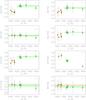 |
Fig. 11 [X/Fe] versus |
| In the text | |
|
Fig. 12 [Fe/H] versus log g for the coolest stars (Teff < 4500 K) of our and D’Orazi et al. re-analyzed samples (stars: ONC; circles: OB1b). |
| In the text | |
|
Fig. 13 [Fe/H] distribution for: SFRs within 500 pc from the Sun (dashed histogram), young nearby loose associations (dot-dashed line), and open clusters younger than 150 Myr and within 500 pc from the Sun (solid line). Sources of [Fe/H] values for the young open clusters are the following: α Persei (Boesgaard & Friel 1990), NGC 2516 (Terndrup et al. 2002), NGC 2451A/B (Hünsch et al. 2004), Blanco 1 (Ford et al. 2005), IC 4665 (Shen et al. 2005), IC 2602 and IC 2391 (D’Orazi & Randich 2009), and Pleiades (Soderblom et al. 2009). |
| In the text | |
|
Fig. B.1 Comparison between continuum flux at λ4900, 5600, 6300, 7500 Å obtained with ATLAS spectra (squares and dashed line) and GAIA spectra (asterisks and dotted line) at log g = 4.0 as a function of Teff. The lines represent an interpolation through the points. |
| In the text | |
|
Fig. B.2 Comparison between continuum flux at the Johnson BVRI-bands obtained with ATLAS spectra (squares and dashed line) and GAIA spectra (asterisks and dotted line) at log g = 4.0 as a function of Teff. The lines represent an interpolation through the points. |
| In the text | |
|
Fig. B.3 Comparison of iron abundances derived by using ATLAS and GAIA model atmospheres as a function of equivalent width (EW) and line excitation potential (EP). These examples display the results obtained for stars with four different temperatures. Circles and asterisks refer to abundances derived with ATLAS and GAIA models, respectively, while solid and dashed lines represent their mean values. Vertical thick and thin bars in the log n(Fe) vs. EW panels are the standard deviations around the average iron abundances. |
| In the text | |
Current usage metrics show cumulative count of Article Views (full-text article views including HTML views, PDF and ePub downloads, according to the available data) and Abstracts Views on Vision4Press platform.
Data correspond to usage on the plateform after 2015. The current usage metrics is available 48-96 hours after online publication and is updated daily on week days.
Initial download of the metrics may take a while.