| Issue |
A&A
Volume 525, January 2011
|
|
|---|---|---|
| Article Number | A35 | |
| Number of page(s) | 22 | |
| Section | Galactic structure, stellar clusters and populations | |
| DOI | https://doi.org/10.1051/0004-6361/201015489 | |
| Published online | 30 November 2010 | |
Online material
Appendix A: Line list
Wavelength, elements, excitation potential, and oscillator strength of all the elements are listed.
Appendix B: Elemental abundance analysis of cool stars: dependence on model atmospheres
Many possible fallacies can affect the process going from the spectroscopic stellar observations to the derivation of the chemical composition using atomic parameters and the derivation of stellar parameters. We focus here on the role of model atmospheres. In particular, we show how the use of different model atmospheres leads to different results in metallicity and other elemental abundances (i.e., sodium, aluminum, silicon, calcium, titanium, and nickel).
B.1. The test
In the following, we present our starting points:
-
We considered three young members of ONC and OB1b (namely,CVSO159, CVSO118, and KM Ori) because theycover a wide range in effective temperature (Teff ~ 4000−4700 K)and surface gravity (log g ~ 3.0−4.5), but our discussion can be extended to alllate-G/early-M stars. We also considered, as a comparison, asolar spectrum acquired by Randichet al. (2006) with flames/uves at asimilar resolution of the other spectra.
-
Abundance analysis was carried out following the steps given in Sect. 4.
-
We considered low-resolution (20 Å) ATLAS2 (Kurucz 1993) and high-resolution (2 Å) GAIA3 (Hauschildt et al. 1999; Brott & Hauschildt 2010, priv. comm.) synthetic spectra to evaluate the continuum flux around lines and in photometric bands normally used for line EW measurements (see Sect. B.2). ATLAS spectra cover the ultraviolet (1000 Å) to infrared (10 μm) spectral range, while GAIA spectra cover the 300 Å ≲ λ ≲ 100 μm wavelength range.
-
Kurucz (1993) and Brott & Hauschildt (2010, priv. comm.) grids of plane parallel model atmospheres were considered for the abundance measurements (see Sect. B.3). ATLAS includes atmosphere models with metallicities −5.0 ≤ [Fe/H] ≤ + 1.0, gravity range 0.0 ≤ log g ≤ 5.0, and 3500 ≤ Teff ≤ 10 000 K. GAIA model atmospheres span in 2000 ≤ Teff ≤ 10 000 K, 0.0 ≤ log g ≤ 5.5, and −4.0 ≤ [Fe/H] ≤ + 0.5. Model atmospheres for specific stellar parameters of our interest were generated by interpolating in the original ATLAS and GAIA grids (see the procedure described by Bean et al. 2006).
B.2. Implications on continuum flux
One of the most important improvements made to the GAIA models was the inclusion of millions of molecular lines in the line list. This is of paramount importance when computing the band opacity, in addition to the line opacity. The effects of band opacities on the continuum flux are most pronounced in the optical domain that is largely used for abundance measurements (namely, 4000–8000 Å).
To help identify the range in effective temperature where the two grids of models can be used for abundance measurements, we calculated the GAIA average continuum fluxes in 20 Å windows centered on λ4900, 5600, 6300, and 7500 Å, which are typical regions used for abundance determinations. These fluxes were evaluated for solar-scaled chemical composition. Continuum flux at the same wavelengths were also considered for ATLAS low-resolution spectra (sampled at 20 Å) of solar abundance. The comparison of these fluxes is shown in Fig. B.1, for log g = 4.0 and for 3000 ≤ Teff ≤ 7500 K, which are a typical gravity and temperatures of low-mass members of star-forming regions. At all temperatures, the flux obtained with the GAIA model is lower than the flux obtained using ATLAS models, but for Teff ≲ 4400 K (depending on the line wavelength) the flux decrement of GAIA spectra is more pronounced than the ATLAS spectra. This is particularly evident, for instance, at λ = 5600, 6300 Å, and is due to the formation in stellar spectra of molecular bands, such as metal oxide (most of all TiO, but also VO), hydroxide (such as OH), hybrids (such as CaH, FeH, MgH) in the visible, and CO and H2O in the near infrared. These bands are not accurately reproduced by ATLAS models, which lack line opacity computations for both triatomic molecules (with the exception of H2O) and numerous diatomic molecular transitions (such as VO).
Since the lines used for abundance measurements are spread over wide spectral ranges (typically in the 4000−8000 Å range), we also calculated the synthetic fluxes in the Johnson BVRI-bands by integrating the synthetic ATLAS and GAIA spectra, weighted by the Johnson transmission curve of the BVRI filters. The results are shown in Fig. B.2 for log g = 4.0. The shift between the ATLAS and GAIA models also appears in the BVRI-fluxes, even if it is less evident than the line-continuum fluxes of Fig. B.1, because of the integration over the band wavelengths.
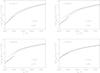 |
Fig. B.1
Comparison between continuum flux at λ4900, 5600, 6300, 7500 Å obtained with ATLAS spectra (squares and dashed line) and GAIA spectra (asterisks and dotted line) at log g = 4.0 as a function of Teff. The lines represent an interpolation through the points. |
| Open with DEXTER | |
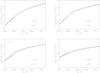 |
Fig. B.2
Comparison between continuum flux at the Johnson BVRI-bands obtained with ATLAS spectra (squares and dashed line) and GAIA spectra (asterisks and dotted line) at log g = 4.0 as a function of Teff. The lines represent an interpolation through the points. |
| Open with DEXTER | |
Examples of Fe, Na, Al, Si, Ca, Ti, and Ni mean abundances obtained for stars in the Orion complex using ATLAS (A) and GAIA (G) models.
B.3. Implications on abundance determination
To search for the effect on abundances, we compared the metallicities and the Na, Al, Si, Ca, Ti, Ni abundances obtained using ATLAS and GAIA models for CVSO159, CVSO118, KM Ori, and the Sun. The results are listed in Table B.1 for both ATLAS and GAIA models.
B.3.1. Iron
The comparison of metallicities is shown in Fig. B.3, where the difference between the two models increases with decreasing temperature, because of the presence of the mentioned bands. In particular, at Teff = 4000−4300 K the difference in abundance is ± 0.07−0.08 dex, while for the Sun the difference is only ± 0.01 dex (see also Table B.1). As a consequence, for a differential abundance analysis with respect to the Sun, for KM Ori (at 4700 K) we do not find almost any difference between the two models, while for both CVSO159 (at 4000 K) and CVSO118 (at 4300 K) the differences are [Fe/H] [Fe/H]
 , + 0.08 dex, respectively. This means that the strong departure of the GAIA model from the ATLAS behavior at ~4400 K shown in Fig. B.1 affects iron abundance, leading to similar differences in stars with
Teff ≲ 4400 K. The lower metallicity resulting from GAIA models (with respect to the ATLAS models) depends on the more signidicant formation of molecules in atmospheres with lower temperatures. The molecular opacity considered in the GAIA models indeed leads to a redistribution of the flux, which is on average lower than the ATLAS one, because of the molecular absorption (line blanketing). Lower flux yields lower intrinsic line equivalent widths, which can be reproduced by lower iron abundances.
B.3.2. Other elements
In Table B.1, we summarize how the use of different models can affect the elemental abundance. Here, the comparison between ATLAS and GAIA grids is listed for Na, Al, Si, Ca, Ti, and Ni. While lines of elements across over the whole spectrum (~4800−6800 Å) infer very different results (such as Ni, besides Fe), elements such as Al, with only two lines at 6696 Å and 6698 Å close each other and not strongly affected by band opacity, lead to similar GAIA and ATLAS abundances.
 |
Fig. B.3
Comparison of iron abundances derived by using ATLAS and GAIA model atmospheres as a function of equivalent width (EW) and line excitation potential (EP). These examples display the results obtained for stars with four different temperatures. Circles and asterisks refer to abundances derived with ATLAS and GAIA models, respectively, while solid and dashed lines represent their mean values. Vertical thick and thin bars in the log n(Fe) vs. EW panels are the standard deviations around the average iron abundances. |
| Open with DEXTER | |
B.4. Concluding...
We find Teff ≈ 4400 K to be the lower limit where the models in which the line opacity computations are not fully treated, such as ATLAS, can be applied in an abundance analysis. This has been demonstrated for both iron abundance, typically derived by many lines, and other elements (α- and iron-peak elements) typically used as tracers of chemical enrichment.
© ESO, 2010
Current usage metrics show cumulative count of Article Views (full-text article views including HTML views, PDF and ePub downloads, according to the available data) and Abstracts Views on Vision4Press platform.
Data correspond to usage on the plateform after 2015. The current usage metrics is available 48-96 hours after online publication and is updated daily on week days.
Initial download of the metrics may take a while.