| Issue |
A&A
Volume 524, December 2010
|
|
|---|---|---|
| Article Number | A6 | |
| Number of page(s) | 33 | |
| Section | Extragalactic astronomy | |
| DOI | https://doi.org/10.1051/0004-6361/201014703 | |
| Published online | 19 November 2010 | |
The fundamental plane of EDisCS galaxies
The effect of size evolution⋆,⋆⋆
1
Max-Planck Institut für extraterrestrische Physik,
Giessenbachstraße,
85741
Garching,
Germany
e-mail: This email address is being protected from spambots. You need JavaScript enabled to view it.
2
Universitäts-Sternwarte München, Scheinerstr. 1, 81679
München,
Germany
3
Departamento de Fisica Teorica, Universidad Autonoma de
Madrid, 28049
Madrid,
Spain
4
Departamento de Astrofísica, Universidad de La
Laguna, 38205 La
Laguna, Tenerife,
Spain
5
Herzberg Institute of Astrophysics, National Research Council of Canada, Victoria,
BC
V9E 2E7,
Canada
6 Spitzer Science Center, Caltech, Pasadena
CA91125, USA
7
School of Physics and Astronomy, University of Nottingham,
University Park, Nottingham
NG7 2RD,
UK
8
Dark Cosmology Centre, Niels Bohr Institute, University of
Copenhagen, Juliane Maries Vej
30, 2100
Copenhagen,
Denmark
9
Osservatorio Astrofisico di Arcetri,
Largo Enrico Fermi 5,
50125
Firenze,
Italy
10
Observatoire de Genève, Laboratoire d’Astrophysique Ecole
Polytechnique Federale de Lausanne (EPFL), 1290
Sauverny,
Switzerland
11
GEPI, Observatoire de Paris, CNRS UMR 8111, Université Paris
Diderot, 92125
Meudon Cedex,
France
12
Institut für Astro- und Teilchenphysik, Universität Innsbruck,
Technikerstr.25/8,
6020
Innsbruck,
Austria
13
Osservatorio Astronomico,
vicolo dell’Osservatorio 5,
35122
Padova,
Italy
14
Ohio University, Department of Physics and
Astronomy, Clippinger Labs
251B, Athens,
OH
45701,
USA
15
INAF, Astronomical Observatory of Trieste,
via Tiepolo 11,
34143
Trieste,
Italy
16
Laboratoire d’Astrophysique de Toulouse-Tarbes, CNRS, Université
de Toulouse, 14 avenue Edouard
Belin, 31400 - Toulouse, France
17
The University of Kansas, Malott room 1082, 1251 Wescoe Hall Drive,
Lawrence, KS
66045,
USA
18
Astronomy Department, University of Padova,
Vicolo dell’Osservatorio 3,
35122
Padova,
Italy
19
Max-Planck-Institut für Astrophysik, Karl-Schwarzschild-Str. 1, Postfach 1317,
85741
Garching,
Germany
20
Steward Observatory, University of Arizona,
933 North Cherry Avenue,
Tucson, AZ
85721, USA
Received:
1
April
2010
Accepted:
2
September
2010
Abstract
We study the evolution of spectral early-type galaxies in clusters, groups, and the field up to redshift 0.9 using the ESO Distant Cluster Survey (EDisCS) dataset. We measure structural parameters (circularized half-luminosity radii Re, surface brightness Ie, and velocity dispersions σ) for 154 cluster and 68 field galaxies. On average, we achieve precisions of 10% in Re, 0.1 dex in log Ie, and 10% in σ. We sample ≈20% of cluster and ≈10% of field spectral early-type galaxies to an I band magnitude in a 1 arcsec radius aperture as faint as I1 = 22. We study the evolution of the zero point of the fundamental plane (FP) and confirm results in the literature, but now also for the low cluster velocity dispersion regime. Taken at face value, the mass-to-light ratio varies as Δlog M/LB = (−0.54 ± 0.01)z = (−1.61 ± 0.01)log (1 + z) in clusters, independent of their velocity dispersion. The evolution is stronger (Δlog M/LB = (−0.76 ± 0.01)z = (−2.27 ± 0.03)log (1 + z)) for field galaxies. A somewhat milder evolution is derived if a correction for incompleteness is applied. A rotation in the FP with redshift is detected with low statistical significance. The α and β FP coefficients decrease with redshift, or, equivalently, the FP residuals correlate with galaxy mass and become progressively negative at low masses. The effect is visible at z ≥ 0.7 for cluster galaxies and at lower redshifts z ≥ 0.5 for field galaxies. We investigate the size evolution of our galaxy sample. In agreement with previous results, we find that the half-luminosity radius for a galaxy with a dynamical orstellar mass of 2 × 10¹¹ M⊙ varies as (1 + z) − 1.0 ± 0.3 for both cluster and field galaxies. At the same time, stellar velocity dispersions grow with redshift, as (1 + z)0.59 ± 0.10 at constant dynamical mass, and as (1 + z)0.34 ± 0.14 at constant stellar mass. The measured size evolution reduces to Re ∝ (1 + z) −0.5 ± 0.2 and σ ∝ (1 + z)0.41 ± 0.08, at fixed dynamical masses, and Re ∝ (1 + z) −0.68 ± 0.4 and σ ∝ (1 + z)0.19 ± 0.10, at fixed stellar masses, when the progenitor bias (PB, galaxies that locally are of spectroscopic early-type, but are not very old, disappear progressively from the EDisCS high-redshift sample; often these galaxies happen to be large in size) is taken into account. Taken together, the variations in size and velocity dispersion imply that the luminosity evolution with redshift derived from the zero point of the FP is somewhat milder than that derived without taking these variations into account. When considering dynamical masses, the effects of size and velocity dispersion variations almost cancel out. For stellar masses, the luminosity evolution is reduced to LB ∝ (1 + z)1.0 for cluster galaxies and LB ∝ (1 + z)1.67 for field galaxies. Using simple stellar population models to translate the observed luminosity evolution into a formation age, we find that massive (>1011 M⊙) cluster galaxies are old (with a formation redshift zf > 1.5) and lower mass galaxies are 3−4 Gyr younger, in agreement with previous EDisCS results from color and line index analyses. This confirms the picture of a progressive build-up of the red sequence in clusters with time. Field galaxies follow the same trend, but are ≈1 Gyr younger at a given redshift and mass. Taking into account the size and velocity dispersion evolution quoted above pushes all formation ages upwards by 1 to 4 Gyr.
Key words: galaxies: elliptical and lenticular, cD / galaxies: evolution / galaxies: formation / galaxies: fundamental parameters
Based on observations collected at the European Southern Observatory, Paranal and La Silla, Chile, as part of the ESO LP 166.A-0162.
Appendices and Tables 1–3 are only available in electronic form at http://www.aanda.org
© ESO, 2010
1. Introduction
Despite their apparent simplicity, the physical processes involved in the formation of early-type galaxies (E/S0) remain unclear. The tightness of their scaling relations, such as the color-magnitude relation, and their slow evolution with redshift, are indicative of a very early and coordinated formation of their stars (e.g., van Dokkum et al. 2000; Blakeslee et al. 2003; Menanteau et al. 2004). However, in the ΛCDM paradigm, these galaxies are expected to form through mergers of smaller subsystems over a wide redshift range, managing to obey these constraints (Kauffmann 1996; De Lucia et al. 2006).
A particularly interesting relation is that of the fundamental plane (hereafter FP). In the
parameter space of central velocity dispersion (σ), galaxy effective radius
(Re), and effective surface brightness
(SBe = −2.5log Ie), elliptical
galaxies occupy a plane, known as the FP (Dressler et al.
1987; Djorgovski & Davis 1987),
which exhibits very little scatter (~0.1 dex). The FP is usually expressed in the form
 (1)where the zero point,
hereafter ZP, is computed from the mean values
(1)where the zero point,
hereafter ZP, is computed from the mean values  ,
,
 , and
, and
 of the sample
 (2)Based on the
assumption of homology, the existence of a FP implies that the ratio of the total mass to
luminosity (M/L) scales with σ and Re. Since
the galaxy M/L depends on both the star formation history of the galaxies and the cosmology,
the study of the FP is a valuable tool for studying the evolution of the stellar population
in early-type galaxies.
(2)Based on the
assumption of homology, the existence of a FP implies that the ratio of the total mass to
luminosity (M/L) scales with σ and Re. Since
the galaxy M/L depends on both the star formation history of the galaxies and the cosmology,
the study of the FP is a valuable tool for studying the evolution of the stellar population
in early-type galaxies.
Several studies of intermediate (z ~ 0.3) and high-redshift (z ~ 0.85) clusters of galaxies have used the ZP shift of the plane to estimate the average formation redshifts of stars in early-type galaxies (e.g., Bender et al. 1998; van Dokkum et al. 1998; Jørgensen et al. 1999; Kelson et al. 2000; van Dokkum & Stanford 2003; Wuyts et al. 2004; Jørgensen et al. 2006). In general, they have all found values compatible with a redshift formation greater than 3. In the field, early studies found slow evolution, compatible with that in clusters (e.g., van Dokkum et al. 2001; Treu et al. 2001; Kochanek et al. 2000). However, evidence of more rapid evolution in the field has been found by other authors (Treu et al. 2002; Gebhardt et al. 2003; Treu et al. 2005a). Taking into account the so-called progenitor bias (for which lower redshift early-type samples contain galaxies that have stopped their star formation only recently and that will not be recognised as early-types at higher redshifts) forces a revision to slightly lower formation redshifts (van Dokkum & Franx 2001, z ≈ 2).
The current view is that both the evolution of early-type galaxies with redshift and the dependence of this evolution on environment differ for galaxies of different mass. These differences manifest themselves as an evolution in the FP coefficient α at increasing redshift, from 1.2 (in the B band) at redshift 0.0 to 0.8 at z ~ 0.8−1.3 (van der Wel et al. 2004; Treu et al. 2005a,b; van der Wel et al. 2005; di Serego Alighieri et al. 2005; Holden et al. 2005; Jørgensen et al. 2006). However, this change in the slope has not been observed at 0.2 < z < 0.8 (e.g., van Dokkum & Franx 1996; Kelson et al. 2000; Wuyts et al. 2004; van der Marel & van Dokkum 2007b; MacArthur et al. 2008). If interpreted as a M-M/L ratio relation, this rotation of the FP indicates that there is a greater evolution in the luminosity of low-mass galaxies with redshift. This interpretation was however questioned by van der Marel & van Dokkum (2007b). Dynamical models provide little evidence of a difference in M/L evolution between low- and high-mass galaxies, and the steepening of the FP may be affected by issues other than M/L evolution, such as an increasing importance of internal galaxy rotation at lower luminosities, not captured by the simple aperture-corrected velocity dispersion used in Eq. (1) (Zaritsky et al. 2008), superimposed on the well known change with redshift in the fraction of S0 galaxies contributing to the early-type population (Dressler et al. 1997; Desai et al. 2007; Just et al. 2010). This so-called rotation of the FP, or change in the tilt of the FP, was originally found in field samples, but Jørgensen et al. (2006) claimed that is also exists for cluster galaxies at z = 0.89.
Most studies of evolution with redshift in cluster early-type galaxies have concentrated on single clusters. It remains unclear whether early-type galaxies in clusters at the same redshift share the same FP, or whether the FP coefficients vary systematically as a function of the global properties of the host cluster (e.g., richness, optical and X-ray luminosity, velocity dispersions, concentration, and subclustering). D’Onofrio et al. (2008) demonstrated that the universality of the FP has yet to be proven and that to avoid causing any biases by comparing the FP relation of clusters at different redshifts a larger number of clusters should be studied.
Furthermore, the ZP evolution of the FP with redshift has been interpreted as an evolution
in the M/L ratio. However, this may not be entirely true if there is a structural evolution
in the size of the galaxies. At face value, observations seem to show that the most massive
(M∗ > 1011 M⊙)
spheroid-like galaxies at z > 1.5, irrespective of
their star-formation activity (Pérez-González et al.
2008) were much smaller (a factor of ~4) than their local counterparts (Daddi et al. 2005; Trujillo et al. 2006, 2007; Longhetti et al. 2007; Zirm et al. 2007; Toft et al. 2007; Cimatti et al. 2008; van Dokkum et al. 2008; Buitrago et al.
2008; Saracco et al. 2009; Damjanov et al. 2009; Ferreras et al. 2009). van Dokkum et al.
(2010) argue that the growth in size with decreasing redshift is due to the
progressive build-up of the outer (R > 5 kpc)
stellar component of galaxies, while the inner core is already in place at redshift ≈2. We
note also that these conclusions have been questioned by Mancini et al. (2010), who find evidence for galaxies as large as local ones at
redshifts higher than 1.4. Complementing our discussion above about the evolution of the
zero point of the FP, if galaxy size were to vary with redshift, we should expect an
accompanying partial revision of the importance of the effect of galaxy size evolution when
taking into account the progenitor bias (Valentinuzzi et al.
2010a). Finally, if a variation in galaxy size with redshift were to occur, we
should expect an accompanying increase in the central velocity dispersion with redshift
(Cenarro & Trujillo 2009; van Dokkum et al. 2009). The evolutions both in size and
velocity dispersion are predicted by theoretical models that take into account internal
feedback “puffing” mechanisms (Biermann & Shapiro
1979; Fan et al. 2008) or the effect of
merging (Khochfar & Silk 2006; Hopkins et al. 2009). As one can read from Eq. (2), a change in ,
, and
with redshift due to
structural evolution will change the amount of stellar population evolution needed to
explain the ZP variation and therefore needs to be taken into account when deriving
constraints on the formation epoch of early-type galaxies.
In this paper, we present the evolution of the FP for a sample of 154 spectral early-type galaxies in 28 clusters or groups and 62 in the field using spectra and images from the ESO Distant Cluster Survey of galaxies (White et al. 2005, EDisCS). The clusters have redshifts between ~0.4 and 0.9 and velocity dispersions between 166 and 1080 km s-1 (Halliday et al. 2004; Clowe et al. 2006; Milvang-Jensen et al. 2008). Our clusters have generally lower velocity dispersions than those typically studied at similar redshifts and represent an intermediate-redshift sample for which a majority of the clusters may be progenitors of typical low-redshift clusters (see Poggianti et al. 2006; Milvang-Jensen et al. 2008).
The paper is organized as follows. Section 2 presents the data set. In particular, Sect. 2.1 describes the measurements of the galaxy velocity dispersions. Section 2.2 describes the measurement of the structural parameters, their errors, and the photometric calibration. Section 2.3 characterizes the statistical properties of the sample. Section 3 presents the FP of EDisCS galaxies. We start in Sect. 3.1 with the FP for 25 clusters and discuss the evolution of the FP zero point as a function of redshift and cluster velocity dispersion. Section 3.2 considers the differences between the FP of galaxies in clusters and the field and the dependence on galaxy mass. Section 3.3 discusses the related problem of the rotation of the FP. In Sect. 4, we consider the size evolution of galaxies and how this affects the stellar population time-dependence implied by the evolution of the FP. In Sect. 5, we draw our conclusions. Appendix A explains in detail how we compute circularized half-luminosity radii. Throughout the paper, we assume that ΩM = 0.3, ΩΛ = 0.7, and H0 = 70 km s-1 Mpc-1.
2. Data analysis
The sample of galaxies analyzed in this paper consists of spectroscopic early-type objects. We considered the flux-calibrated spectra reduced in Halliday et al. (2004) and Milvang-Jensen et al. (2008) of galaxies with early spectral type (1 or 2). This indicates the total absence (type 1) or the presence of only weak (with equivalent width smaller than 5 Å) [OII] lines (Sánchez-Blázquez et al. 2009). We derive galaxy velocity dispersions from these spectra (Sect. 2.1). We match this dataset with HST and VLT photometry (Sect. 2.2). The HST images (Desai et al. 2007) provide visual classification and structural parameters for 70% of our galaxies. For the remaining 30%, we use VLT photometry, where no visual classification is available (Simard et al. 2009). Approximately 70% of the galaxies with HST photometry have early-type morphologies (Sect. 2.3).
2.1. Velocity dispersions
Velocity dispersions were measured in all galaxy spectra using the IDL routine pPXF (Cappellari & Emsellem 2004). This routine is based on a maximum penalized likelihood technique that employs an optimal template, and also performs well when applied to spectra of low signal-to-noise ratio (Cappellari et al. 2009). The algorithm works in pixel space, estimating the best fit to a galaxy spectrum by combining stellar templates that are convolved with the appropriate mean galaxy velocity and velocity dispersion. The results depend critically on how well the spectra are matched by the template. To compile an optimal template, we use 35 synthetic spectra from the library of single stellar-population models of Vazdekis et al. (2010), which uses the new stellar library MILES (Sánchez-Blázquez et al. 2006). These spectra were degraded to the wavelength-dependent resolution of the EDisCS spectra, determined from the widths of the lines in the arc lamp spectra, slit by slit, which match well the widths of the sky lines in the science spectra.
The library contains spectra spanning an age range from 0.13 to 17 Gyr and metallicities from [ Z/H ] = −0.68 to [ Z/H ] = +0.2. Operating in pixel space, the code allows the masking of regions of the galaxy spectra during the measurements. We use this to mask regions affected by skyline residuals. Although the code allows the measurement of the higher Gauss-Hermite order moments (Bender et al. 1994), we only fit the velocity and σ, which helps to stabilise the fits in our spectra of low signal-to-noise ratio. Errors were calculated by means of Monte Carlo simulations in which each point was perturbed with the typical observed error, following a Gaussian distribution. Because the template mismatch affects the measurement of the velocity and σ determined with pPXF, a new optical template was used in each simulation. The errors were assumed to be the standard deviation in measurements inferred from 20 simulations. Owing to limitations caused by the instrumental resolution, only velocity dispersions larger than 100 km s-1 are reliable and unbiased. Therefore, galaxies with smaller σ, as well as velocity dispersions with uncertainties larger than 20%, the approximate intrinsic scatter of the local FP (see Introduction), are not be considered any further.
We note that the velocity dispersions measured here are ≈10% lower than those given in Sánchez-Blázquez et al. (2009). The difference is caused by the instrumental resolution in that paper having been assumed to be constant with wavelength at the value of 6 Å. In reality, this is only the optimal resolution possible with our setup, which can be as large as 8 Å. The change is important here, but does not affect any of the results presented in Sánchez-Blázquez et al. (2009).
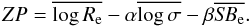
We measured velocity dispersions for 192 cluster and 78 field galaxies. Figure 1 shows the histograms of the statistical errors. The statistical errors are on average 10% and are a function of magnitude.
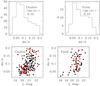 |
Fig. 1 The velocity dispersion errors. First row: the histograms of statistical errors on velocity dispersions. Second row: the statistical errors as a function of apparent I band magnitude in a 1 arcsec radius aperture. Colors code the spectroscopic type (black: 1; red: 2). |
The systematic errors are more difficult to estimate, as they depend on the template mismatch, continuum variations, and filtering schemes. They have been extensively studied in the past (Cappellari & Emsellem 2004) and can be as large as 5−10%. To determine the size of the systematic errors, we derived the galaxy velocity dispersions using the FCQ method of Bender et al. (1994), which is less prone to template mismatching systematics and operates in Fourier space. We focused on the G band region at z ≈ 0.5, the Mgb region at lower redshifts, or the largest available continuous range redder than the 4000 Å break, similar to the approach of Ziegler et al. (2005). The two methods agree well, with 68% of the values differing by less than the combined 1-σ error, and 96% by less than 3-σ, but smaller errors are derived using the pixel fitting approach, partially because most of each spectrum can be used. This allows us to conclude that our residual systematic errors are always smaller than the statistical ones.
Finally, an aperture correction following Jørgensen
et al. (1995) (3)where Ap represents
the average aperture of our observations, 1.15 arcsec, scaled with the distances of the
objects, was applied to the measured velocity dispersions σmes
to place them on the Coma cluster standard aperture system of 3.4 kpc. Figure 2 shows that, on average, this correction amounts to 3%
with ≈0.5% spread. From this point on, we drop the cor and indicate
with σ the aperture-corrected value of the velocity dispersion.
(3)where Ap represents
the average aperture of our observations, 1.15 arcsec, scaled with the distances of the
objects, was applied to the measured velocity dispersions σmes
to place them on the Coma cluster standard aperture system of 3.4 kpc. Figure 2 shows that, on average, this correction amounts to 3%
with ≈0.5% spread. From this point on, we drop the cor and indicate
with σ the aperture-corrected value of the velocity dispersion.
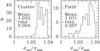 |
Fig. 2 The histogram of the fractional aperture corrections σcor/σmes for cluster (left) and field (right) galaxies. |
Figure 3 presents the velocity dispersions as a function of redshift and their distribution. On average, the galaxy velocity dispersion is ≈200 km s-1, with a mildly increasing trend with redshift. Weighting each galaxy by the inverse of its completeness value (see Sect. 2.3) in general changes the mean by no more than its error.
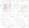 |
Fig. 3 The velocity dispersions of the galaxy sample. Top: the measured galaxy velocity dispersions as a function of redshift in clusters (left) and the field (right). The green lines show the mean values in 0.1 redshift bins and the relative errors. The dotted lines show the mean values weighting each galaxy with the inverse of its completeness value. Bottom: the histogram of galaxy velocity dispersions in clusters (left) and the field (right). Colors code the spectral type (black: 1; red:2). The dotted lines show the histogram for the entire sample irrespective of spectral type. |
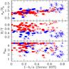 |
Fig. 4 The properties of the bulge+disk fits to galaxies with HST photometry and a measured velocity dispersion. We plot the ratio ae/Re of the semi-major effective scale length ae of the best-fit Sersic profile to the circularized effective radius Re of the best-fit B+D model (top), the bulge-to-total ratio B/T (middle), and the Sersic index nSer (bottom) as a function of the ellipticity 1 − be/ae (where be is the semi-minor effective scale length) of the Sersic fit. Objects with B/T > 0.5 are plotted in red, the remainder in blue. Symbols code the morphology: filled ellipses show T ≤ −4, filled circles crossed by a line −3 ≤ T ≤ 0, spirals T > 0. |
2.2. Photometry
The photometric part of the FP, i.e., the half-luminosity radius
Re and average effective surface brightness
 ,
where L is the total luminosity, was derived by fitting either HST ACS
images (Desai et al. 2007) or
I-band VLT images (White et al.
2005) using the GIM2D software (Simard et al.
2002). Simard et al. (2009) provide an
extensive description of the methods and tests performed to assess the accuracy of the
derived structural parameters, using exhaustive Monte Carlo simulations. To summarize, a
two-component two-dimensional fit was performed, adopting an
R1/4 bulge plus an exponential disk
convolved to the PSF of the images. From the parameters of the fit, we measured the
(circularized) Re and effective surface brightness from curves
of growth constructed from the best-fit models using the procedure described in
Appendix A.
,
where L is the total luminosity, was derived by fitting either HST ACS
images (Desai et al. 2007) or
I-band VLT images (White et al.
2005) using the GIM2D software (Simard et al.
2002). Simard et al. (2009) provide an
extensive description of the methods and tests performed to assess the accuracy of the
derived structural parameters, using exhaustive Monte Carlo simulations. To summarize, a
two-component two-dimensional fit was performed, adopting an
R1/4 bulge plus an exponential disk
convolved to the PSF of the images. From the parameters of the fit, we measured the
(circularized) Re and effective surface brightness from curves
of growth constructed from the best-fit models using the procedure described in
Appendix A.
Historically, effective radii were derived from fits to curves of growths, constructed from photoelectric photometry using circular apertures of increazing sizes (Burstein et al. 1987). Our procedure reproduces this approach and is identical to that followed by Gebhardt et al. (2003) to study the evolution of the FP of field galaxies with redshift. We prefer it to less sophisticated approaches (such as the straight R1/4 fit often used in the literature) as it provides far superior fits to the images. As Gebhardt et al. (2003) do, we note that in the past a variety of methods have been adopted to measure the structural parameters that enter into the FP: curve of growth, isophotal photometry, or 2-dimensional fitting, pure R1/4, Sersic, or bulge+disk (B+D) functions. The derived effective radii and surface brightness, however, when combined in Eq. (1) of the FP, deliver the same ZP to a high degree of accuracy (Saglia et al 1993). This has been proven for a large set of local clusters, including the Coma cluster (Saglia et al. 1997b; de Jong et al. 2004), and remains valid for the present data set (see below). This justifies the comparisons with FP samples from the literature presented below.
We later use effective radii to probe the size evolution of galaxies. Without a doubt, the scale length along the major axis of a pure disk galaxy is the correct measurement of its size, and our circularized Re progressively underestimates the effective semi-major axis length as the inclination increases (see Fig. 4). However, for a pure bulge the inverse is true, and our Re then averages out projection effects, producing the equivalent circularized size of each spheroid.
On the other hand, both the resolution and signal-to-noise ratio of the images considered here are too low to allow us to perform an accurate and unbiased determination of the sizes of the bulge and the disk components separately for our galaxies. Since the percentage of disk-dominated, highly inclined objects in the galaxy sample considered here is low, as it is in the low redshift comparison, we conclude that our choice is reasonable. In particular, the mean axial ratios of our sample and the low redshift comparison are identical, as discussed in Valentinuzzi et al. (2010b).
We now consider the quantitative question of the extent to which our procedure for computing structural parameters is equivalent to other approaches discussed in the literature.
In analogy with procedures followed for local galaxies (Saglia et al. 1997a), where systematic errors are gauged by comparing different photometric fits, we assess the robustness of the structural parameters to the chosen R1/4 bulge plus exponential disk surface brightness model by considering a second two-dimensional fitting approach to the HST images. We fit a single-component Sersic profile (with 0.5 ≤ nSer ≤ 4.5) to the HST ACS imaging in the F814W band, available for 10 of the EDisCS clusters. Again, the circularized half-luminosity radius Re(Ser) is computed from curves of growth constructed from the best-fit model as described in Appendix A.
Figure 4 summarizes the results of our B+D and Sersic fits. The galaxies of our HST sample have on average a flattening 1 − be/ae of 0.37 (0.33 without spirals), with some disk-dominated, nearly edge-on spiral galaxies reaching 1 − be/ae ≈ 0.8. As a consequence, our circularized effective radii are on average 39% (33% without spirals) smaller than the effective semi-major lengths ae. On average, our objects are bulge-dominated (⟨ B/T ⟩ = 0.59, 0.64 without spirals) and reasonably well described by a de Vaucouleurs law (⟨ nSer ⟩ = 3.7, 3.9 without spirals).
Figures 5 − 7
(top and middle panels) assess the robustness of the derived structural parameters derived
for the galaxies with measured velocity dispersions. For this purpose, we also consider
the harmonic radius
Rhar = (aebe)1/2,
often used in the literature as a proxy for Re (sometimes
fixing the Sersic index to 4, the R1/4 law)
and the related average surface brightness  , where ae and
be are the effective semi-major and minor axis of the Sersic
fits. The evaluated harmonic and circularized Sersic radii are on average very similar to
our adopted Re, as well as the resulting effective surface
brightness. When combined into the quantity orthogonal to the FP
log Re − 0.27 ⟨ SBe ⟩ , they
show minimal systematic differences and scatter. As discussed in Appendix A, only at high flattening (i.e. for almost edge-on
disk-dominated galaxies) do the harmonic quantities show the expected stronger deviations.
, where ae and
be are the effective semi-major and minor axis of the Sersic
fits. The evaluated harmonic and circularized Sersic radii are on average very similar to
our adopted Re, as well as the resulting effective surface
brightness. When combined into the quantity orthogonal to the FP
log Re − 0.27 ⟨ SBe ⟩ , they
show minimal systematic differences and scatter. As discussed in Appendix A, only at high flattening (i.e. for almost edge-on
disk-dominated galaxies) do the harmonic quantities show the expected stronger deviations.
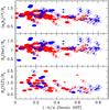 |
Fig. 5 The comparison between different estimations of the half-luminosity radii of all galaxies with HST photometry and a measured velocity dispersion. We plot the ratio of the harmonic radius (aebe)1/2 to the circularized effective radius Re of the best-fit HST B+D model (top), the ratio of the circularized effective radius Re(Ser) of the Sersic fit to Re (middle), and the ratio of the circularized effective radius Re(VLT) of the best-fit VLT B+D model to Re (bottom) as a function of 1 − be/ae. Symbols and color coding are as in Fig. 4. |
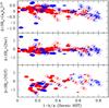 |
Fig. 6 The comparison between different estimates of the effective surface brightness of all galaxies with HST photometry and a measured velocity dispersion. We plot the difference Δ ⟨ SBe(aebe) ⟩ between the average surface brightness within (aebe)1/2 and Re (top), the difference Δ ⟨ SBe(Ser) ⟩ between the average surface brightness within Re(Ser) and Re (middle), and the difference between the average surface brightness within Re(VLT) and Re (bottom) as a function of 1 − be/ae. Symbols and color coding are as in Fig. 4. |
In summary, the median differences are small (the Sersic Re are 9% larger, the Sersic effective surface brightnesses are ≈0.13 mag brighter). The widths at the 68% percentile of the distributions are δ68log Re ~ 0.07, δ68 ⟨ SBe ⟩ ~ 0.24, and δ68FP ~ 0.005 for cluster and (slightly smaller for) field galaxies with measured velocity dispersions. Given the quality of our HST ACS images, we conclude that we measure the structural parameters of galaxies with a precision similar to that of local galaxies (Saglia et al. 1997b; de Jong et al. 2004).
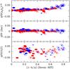 |
Fig. 7 The comparison between different estimations of the quantity FP = log Re − 0.27 ⟨ SBe ⟩ for all galaxies with HST photometry and a measured velocity dispersion. We plot ΔFP(aebe)1/2 = log ((aebe)1/2/Re) − 0.27(⟨ SBe ⟩ (aebe)1/2) − ⟨ SBe ⟩ ) (top), ΔFP = log (Re(Ser)/Re) − 0.27(⟨ SBe ⟩ (Ser) − ⟨ SBe ⟩ ) (middle), and ΔFP = log (Re(VLT)/Re) − 0.27(⟨ SBe ⟩ (VLT) − ⟨ SBe ⟩ ) (bottom) as a function of 1 − be/ae. Symbols and color coding are as in Fig. 4. |
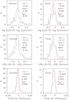 |
Fig. 8 The quality of the photometry parameters derived from HST images for cluster (left) and field (right) galaxies. We show histograms of the differences between structural parameters derived from bulge plus disk (B+D) and Sersic GIM2D fits to the HST ACS images of the galaxies with measured velocity dispersions. The mean, rms, and the widths at the 68% percentile of the distributions are given. |
For the remaining clusters with only ground-based images, we derive the structural parameters as described above (Simard et al. 2009), i.e., by fitting an R1/4 bulge plus an exponential disk 2D model to the I-band VLT deep images that were obtained in excellent seeing conditions. Circularized half-luminosity radii are derived from curves of growth constructed from the best fits as described in Appendix A. In general, simulations show that the structural parameters derived from the fits to VLT images are of reasonably good precision when nearly-isolated galaxies (i.e., those for which the segmentation area has little contamination from nearby objects) are considered. Statistical errors smaller than 0.27 mag in total magnitudes and smaller than 0.36 dex in log Re are derived, in addition to systematic errors smaller than 0.15 mag and 0.2 dex, respectively, if bright objects (Imag < 22.5) are examined (Simard et al. 2009). The galaxies in our sample are typically at least one magnitude brighter than this limit.
The bottom panels of Figs. 5–7 show the comparison of the VLT-derived structural parameters with the HST-derived structural parameters as a function of galaxy flattening, while Fig. 9 shows the histograms of the differences δlog Re = log Re(HST) − log Re(VLT), δ ⟨ SBe ⟩ = ⟨ SBe ⟩ (HST) − ⟨ SBe ⟩ (VLT), and δFP = δlog Re − 0.27δ ⟨ SBe ⟩ for objects with measured velocity dispersions where HST images are also available. For cluster objects that are isolated or have only relatively small companions (SExtractor flags 0 or 2, Bertin & Arnouts 1996), the comparison is reasonable, with median ⟨ δlog Re ⟩ med ~ −0.08, δ68log Re ~ 0.14, (i.e., VLT half-luminosity radii are on average 20% larger than HST Re with ≤ 25% scatter), and median difference ⟨ δ ⟨ SBe ⟩ ⟩ med ~ − 0.32, δ68 ⟨ SBe ⟩ ~0.53 (i.e., VLT effective surface brightnesses are on average 0.32 mag brighter than those from HST ⟨ SBe ⟩ with ≤ 0.53 mag scatter). The errors δlog Re and δ ⟨ SBe ⟩ are correlated, with minimal scatter in the direction almost orthogonal to the FP, i.e., δFP = δlog Re −0.27δ ⟨ SBe ⟩ and δ68FP ~ 0.025 and there is a small median shift. No trend with redshift is seen. These values agree with or are of higher precision than those derived from simulations (see above). Very similar results are obtained for field objects. Therefore, the VLT dataset can be merged with the HST-based one to study the evolution of the FP (Sect. 3).
The systematic and random errors increase dramatically if objects with sizable companions (VLT SExtractor flag 3) are considered. In these cases, the VLT segmentation areas fitted by GIM2D are heavily contaminated by the companions. As a consequence, Re(VLT) and VLT total magnitudes are systematically larger and brighter, respectively, than those derived from HST fits. There are 38 cluster and 10 field galaxies with early spectral type and measured velocity dispersion that have only VLT imaging and a SExtractor flag equal to 3. Given the already sizeable systematics in Re detected for the “isolated” objects, we refrain from attempting an iterative fit and just exclude the affected galaxies from the FP analysis.
In Sect. 4, we use the half-luminosity radii discussed above to constrain the size evolution of our galaxies. The high-precision (≈10% systematic) HST half-luminosity radii are certainly good enough and our results are based on this dataset only. A number of caveats have to be kept in mind when considering the VLT radii. According to the Monte Carlo simulations discussed by Simard et al. (2009, Fig. 1), the VLT radii of the largest galaxies of the sample (larger than 1.8 arcsec) may underestimate the true radii by up to 40%. But only 2.5% of our sample has Re > 1.8′′. Sizes smaller than 0.1 arcsec are probably unreliable because of the limits to our resolution, but only 3% of cluster galaxies and 5% of field galaxies fall into this category. Finally, if galaxies have strong color gradients, our half-luminosity radii, derived from I band images (i.e., approximately rest-frame V band at redshift 0.5 and rest-frame B band at redshift 0.8) might be affected differentially with redshift. However, we do not detect any significant trend with redshift in the sizes derived from our VLT B and V band images relative to the ones used here from the I band images. Despite all these systematic differences between HST and VLT Re radii (on average 20%), Sect. 4 shows that the size evolution derived from VLT Re radii is very similar.
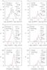 |
Fig. 9 The quality of the photometry parameters derived from VLT images for cluster (left) and field (right) galaxies. Histograms of the differences between structural parameters derived from bulge plus disk GIM2D fits to the HST ACS and VLT I band images of the isolated, undisturbed galaxies with measured velocity dispersions. The mean, rms, and the widths at the 68% percentile of the distributions are given. |
As a last step, effective surface brightnesses were calibrated as follows. Corrections to rest-frame Johnson B band were applied based on the spectroscopic redshift z and an interpolation of the best-fit spectral energy distribution, using our photometric redshift procedure (Rudnick et al. 2009; Pelló et al. 2009). Moreover, the Tolman correction (1 + z)4 was taken into account. Finally, to be able to compare our results with those of Wuyts et al. (2004) and related papers, we transformed effective surface brightness to surface brightness at Re using a conversion factor that is valid for a pure R1/4 law, i.e., Ie = ⟨ Ie ⟩ /3.61 and log ⟨ Ie ⟩ (L⊙/pc2) = − 0.4(⟨ SBe ⟩ − 27).
Figure 10 shows log Re,
log Ie, and dynamical mass
log Mdyn as a function of redshift. Following van Dokkum & van der Marel (2007), we compute
dynamical masses to be  (4)(see also
Sect. 3.2). The mean size of the half-luminosity
radius remains approximately constant at values of ≈2.5 kpc. In contrast, the surface
brightness at Re increases on average by a factor 2 from
redshift 0.4 (where it is
≈250 L⊙/pc2) to redshift
0.8. This matches the differential luminosity evolution inferred from the FP zero-point
evolution with redshift (see Sect. 3.1). Weighting
each galaxy with the inverse of its selection value to correct for incompleteness (see
Sect. 2.3) pushes the sample averages of
log Re and log Ie to slightly
lower and higher values, respectively. As for the velocity dispersions, the effect is
however on the order of the error in the averages. We note that the situation changes when
we consider the size evolution of mass-selected samples (see Sect. 4). We study cluster galaxies with dynamical masses higher than
1.5 × 10¹⁰ M⊙ and field galaxies with
dynamical masses higher than 2.5 × 10¹⁰ M⊙.
Both cluster and field galaxies have on average a dynamical mass of
1011 M⊙.
(4)(see also
Sect. 3.2). The mean size of the half-luminosity
radius remains approximately constant at values of ≈2.5 kpc. In contrast, the surface
brightness at Re increases on average by a factor 2 from
redshift 0.4 (where it is
≈250 L⊙/pc2) to redshift
0.8. This matches the differential luminosity evolution inferred from the FP zero-point
evolution with redshift (see Sect. 3.1). Weighting
each galaxy with the inverse of its selection value to correct for incompleteness (see
Sect. 2.3) pushes the sample averages of
log Re and log Ie to slightly
lower and higher values, respectively. As for the velocity dispersions, the effect is
however on the order of the error in the averages. We note that the situation changes when
we consider the size evolution of mass-selected samples (see Sect. 4). We study cluster galaxies with dynamical masses higher than
1.5 × 10¹⁰ M⊙ and field galaxies with
dynamical masses higher than 2.5 × 10¹⁰ M⊙.
Both cluster and field galaxies have on average a dynamical mass of
1011 M⊙.
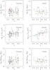 |
Fig. 10 The distribution with redshift of sizes, surface luminosities, and dynamical masses
of the galaxy sample. We show the half-luminosity radii
log Re (top), effective surface
brightness log Ie (middle), and
dynamical mass log Mdyn (bottom) as a
function of redshift for cluster (left) and field
(right) galaxies. Black and red points show spectroscopic types 1
and 2, respectively. Crosses and circles show galaxies with HST and VLT photometry,
respectively. The solid green lines show the mean values in 0.1 redshift bins with
the errors. The dotted lines show the averages obtained by weighting each galaxy
with the inverse of its selection value. The blue lines show the mean luminosity
evolution derived from Fig. 17:
|
2.3. Selection function
Figure 11 describes the final sample. We measured velocity dispersions for 113 cluster and 41 field spectral early-type galaxies with HST photometry, and 41 cluster and 27 field galaxies with only VLT good photometry. A large fraction of galaxies with HST photometry also have early-type morphology: 67% of the objects in clusters and 78% in the field were classified as either Es or S0. Moreover, 77% of galaxies in clusters and 68% in the field do not exhibit [OII] emission, being of spectral type 1.
 |
Fig. 11 Statistics of the sample of galaxies with measured velocity dispersions and photometric parameters. |
To quantify the selection function of our sample, we assign a selection probability PS to each galaxy. This is computed in two steps. First, the σ-completeness probability Pσ of the velocity dispersion measurements is determined. This is shown in Fig. 12. For each given spectral type, we compute the ratio of the number of galaxies with a measured velocity dispersion and reliable photometric structural photometry (see above) to the number of galaxies with a spectrum in a given magnitude bin. In a way similar to Milvang-Jensen et al. (2008), we use the I band magnitude in a 1 arcsec radius aperture I1. We compute these curves separately for cluster and field galaxies, and for galaxies with redshifts either equal to or lower than or higher than 0.6. Finally, we assign the probability Pσ(I1,z,ST,F/C) to each galaxy by linearly interpolating the appropriate curve for its redshift z, spectral type ST, and field or cluster environment (F/C) as a function of magnitude. The σ-completeness is high at bright magnitudes and declines toward fainter objects. In this regime, the σ completeness is also slightly higher for higher redshift galaxies, where the exposure times are longer. The differences between cluster and field galaxies are not as pronounced.
 |
Fig. 12 The relative completeness functions. The fraction of galaxies with an observed spectrum of spectroscopic type 1 or 2 for which we could measure velocity dispersions and obtain reliable photometric structural parameters. This relative completeness is shown for the clusters (top row) and the field (bottom row) as a function of galaxy magnitude in the I band in a 1 arcsec radius aperture. Colors code the spectral type (black: 1; red: 2). The full lines indicate the full redshift range, the dotted lines galaxies with z < 0.6, and the dashed lines galaxies with z ≥ 0.6. The dots show the magnitudes of the single galaxies and the assigned completeness weight. |
As a second step, following Milvang-Jensen et al.
(2008) we consider the total number of spectroscopically targeted galaxies
NT(drawn from a photometric magnitude-limited sample far
deeper than that considered here; see Milvang-Jensen
et al. 2008) in a given magnitude bin, separately for each of the 19 fields we
observed. In the given field, we then consider the number of galaxies for which we were
able to derive a secure redshift NR (with a success rate of
essentially 100%; see Milvang-Jensen et al. 2008),
the number of galaxies spectroscopically found to be members of any cluster
NC, and the number of galaxies found in the field,
NF = NR − NC.
We construct the ratio functions  and
and
 and
interpolate them at the magnitude of each galaxy. Finally, we assign to each galaxy the
selection probability
PS(Cluster) = Pσ × RC
or
PS(Field) = Pσ × RF
if the galaxy belongs to a cluster or to the field.
and
interpolate them at the magnitude of each galaxy. Finally, we assign to each galaxy the
selection probability
PS(Cluster) = Pσ × RC
or
PS(Field) = Pσ × RF
if the galaxy belongs to a cluster or to the field.
Figure 13 shows the resulting probabilities as a function of I1 and dynamical mass (see Eq. (4) and Sect. 3.2). In clusters, we sample between 10% and 30% of the spectral early-type population. The selection probability is almost flat as a function of mass for Mdyn ≥ 4 × 10¹⁰ M⊙. This is above the stellar mass completeness limit of our parent stellar catalogue. In this mass range, the selection probability has no dependence on the galaxy colors. We become progressively more incomplete at lower masses, where we sample just 10% of the population. The effect is less pronounced at higher redshifts. In the field, the average completeness is lower (≈15%) and similar trends are observed. In general, Pσ traces PS quite well, with PS ≈ (0.29 ± 0.12)Pσ. In the abstract and in the following, we quote first results obtained by ignoring selection effects, and then illustrate the effect of the selection correction.
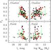 |
Fig. 13 The completeness function of the galaxy sample. The completeness weight for the galaxies with a velocity dispersion for clusters (top row) and the field (bottom row). Left: as a function of galaxy magnitude in the I band in a 1 arcsec radius aperture; right: as a function of dynamical mass. Colors code the spectral type (black: 1; red: 2). Filled circles show galaxies with redshift either equal to or higher than 0.6, open circles galaxies with redshift lower than 0.6. The green full lines with error bars show the bin averages and rms over the full redshift range. The dotted lines refer to the sample with z < 0.6, the dashed lines to the sample with z ≥ 0.6. |
Tables 1 and 2 summarize the velocity dispersions and the structural parameters of the cluster and field galaxies, respectively. For each galaxy, we list its name (White et al. 2005), the number of the cluster to which it belongs (if it is a cluster galaxy, see Table 4 for the correspondence between cluster name and number), spectroscopic redshift and type (Halliday et al. 2004; Milvang-Jensen et al. 2008), raw and aperture-corrected velocity dispersion σmes and σcor with estimated statistical error, circularized half-luminosity radius Re, surface brightness log Ie in the rest-frame B-band, and, when HST images are available, morphological type. When VLT-only images are available, the morphological flag is set to be ∗ when the SExtractor flag is equal to 3, i.e., when the photometric parameters are expected to be contaminated by companions. Moreover, we list the selection probabilities PS and the stellar masses (see Sect. 3.2). In addition, Table 3 gives the circularized Re and log Ie derived from Sersic fits (to HST images) and bulge+disk fits to VLT images for the galaxies for which both HST and VLT images are available.
3. The fundamental plane of the EDisCS galaxies
3.1. The FP of EDisCS clusters
Figure 14 shows the FP of the 14 EDisCS clusters
with HST photometry, while Fig. 15 provides the FP
of the additional 12 clusters with VLT-only photometry. In each cluster, good FP
parameters are available for only a small number of galaxies
(<9), the exceptions being cl1232.5-1144, cl1054.4-1146,
cl1054.7-1245, and cl1216.8-1201. Therefore, at this stage we do not attempt to fit the
parameters of the FP except for the zero point, keeping the velocity dispersion and
surface brightness slopes fixed to the local values (α0 = 1.2,
β0 = −0.83/(−2.5) = 0.33, Wuyts et al. 2004). In Sect. 3.3, we argue that this is a good approximation up to redshift 0.7.
Following van Dokkum & van der Marel
(2007), we compute the zero point as  (5)where
the sum comprises all N galaxies in a cluster with measured velocity
dispersion, early spectroscopic type (1 or 2), and (for clusters with only VLT photometry)
SExtractor flag 0 or 2, irrespective of morphology. At this stage, we weight each point by
w = (1/1.2dσ)2, where
dσ is the error in σ, and do not apply
selection-weighting to be consistent with the procedures adopted in the literature and to
minimize scatter. We note that this could generate systematic differences, given that the
considered surveys have different selection functions. We explore below the influence of
our selection function on the results. The error in the zero point is
δZP = rms(ZP)/
(5)where
the sum comprises all N galaxies in a cluster with measured velocity
dispersion, early spectroscopic type (1 or 2), and (for clusters with only VLT photometry)
SExtractor flag 0 or 2, irrespective of morphology. At this stage, we weight each point by
w = (1/1.2dσ)2, where
dσ is the error in σ, and do not apply
selection-weighting to be consistent with the procedures adopted in the literature and to
minimize scatter. We note that this could generate systematic differences, given that the
considered surveys have different selection functions. We explore below the influence of
our selection function on the results. The error in the zero point is
δZP = rms(ZP)/ .
.
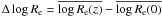
Following Wuyts et al. (2004), we use the Coma cluster as a reference point for the whole sample with ZP = 0.65. All past studies measuring the peculiar motions of the local universe of early-type galaxies (Lynden-Bell et al. 1988; Colless et al. 2001; Hudson et al. 2004, and references therein) agree with the conclusion that Coma, the richest and, in the FP context, the most well-studied local cluster, is at rest with respect to the cosmic microwave background and therefore the best suited as a reference. We convert the variation in the FP zero point into a variation in the mean mass-to-light ratio of galaxies in the B band with respect to Coma using the relation Δlog M/LB = (ZP − 0.65)/0.83 (where 0.83 = β0 × 2.5, see Eqs. (7) and (8)). We note that at this stage we still implicitly assume, as in the past, that no evolution in size or velocity dispersion is taking place. Figure 16, left, shows Δlog M/LB as a function of redshift. Only clusters with 4 or more (N ≥ 4) galaxies are considered. Table 4 gives the relevant quantities: cluster number (Col. 1), cluster name (Col. 2, from Milvang-Jensen et al. 2008), cluster short name (Col. 3), type of photometry used (HST or VLT, Col. 4), cluster velocity dispersion (Col. 5), Δlog M/LB (Col. 6), scatter (Col. 7), and number of galaxies considered (Col. 8). Table 4 also lists the first six columns for the remaining clusters without FP ZPs. If we compute Δlog M/LB using the VLT photometry for the 12 clusters with both HST and VLT photometry, we derive a mean value Δlog M/LB(VLT − HST) = −0.04 (−0.02 if two outliers, CL1354 and CL1138, are not considered) with an rms of 0.06 or an error in the mean of 0.02 (see also Sect. 3.2).
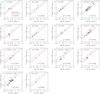 |
Fig. 14 The FP of the EDisCS clusters with HST photometry. Each cluster is identified by its short name for clarity, see Table 4 for the full name. Colors code the spectroscopic type (black = 1, red = 2). Symbols code the morphology: filled ellipses show T ≤ − 4, filled circles crossed by a line − 3 ≤ T ≤ 0, spirals T > 0. The magenta line shows the best-fit FP relation with no selection weighting. The full line shows the Coma cluster at zero redshift. The black dotted and dashed lines show data for the clusters MS2053-04 at z = 0.58 and MS1054-03 at z = 0.83, respectively, from Wuyts et al. (2004). |
 |
Fig. 15 The FP of the EDisCS clusters with VLT only photometry. Each cluster is identified by its short name for clarity, see Table 4 for the full name. Colors code the spectroscopic type. The black squares show galaxies with SExtractor flags different from 0 or 2 and therefore unreliable photometric parameters. The dotted magenta line shows the best-fit FP relation for all galaxies. The solid magenta line shows the best-fit FP relation when considering only galaxies with spectroscopy type ≤ 2 and SExtractor flag 0 or 2. The full line shows the Coma cluster at zero redshift. The black dotted and dashed lines show the clusters MS2053-04 at z = 0.58 and MS1054-03 at z = 0.83 from Wuyts et al. (2004), respectively. |
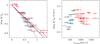 |
Fig. 16 Left: the redshift evolution of the B band mass-to-light ratio. The full black lines show the simple stellar population (SSP) predictions for a Salpeter IMF and formation redshift of either zf = 2 (lower) or 2.5 (upper curve) and solar metallicity from Maraston (2005). The blue line shows the SSP for zf = 1.5 and twice-solar metallicity, the magenta line the SSP for zf = 2.5 and half-solar metallicity. The dotted line shows the best-fit linear relation and the 1σ errors dashed. Right: the (absence of) correlation of the M/L residuals Δlog M/LB + 0.54z with cluster velocity dispersion. Black points are EDisCS clusters with HST photometry, cyan points with VLT photometry. Each EDisCS cluster is identified by its short name for clarity, see Table 4 for the full name. Red points are from the literature, Bender et al. (1998) and van Dokkum & van der Marel (2007). Cluster velocity dispersions come from Halliday et al. (2004) and Milvang-Jensen et al. (2008) for EDisCS clusters and from Edwards et al. (2002) (Coma), Le Borgne et al. (1992) (A2218), Gómez et al. (2000) (A665), Carlberg et al. (1996) (A2390), Fisher et al. (1998) (CL1358+62), Mellier et al. (1988) (A370), Poggianti et al. (2006) (MS1054-03 and CL0024+16), van Dokkum & van der Marel (2007) (3C 295, CL1601+42, CL0016+16), Tran et al. (2005) (MS2053-04), Jørgensen et al. (2005) (RXJ0152-13), and Jørgensen et al. (2006) (RXJ1226+33) for the literature clusters. We estimate σclus for RDCS1252-29 and RDCS084+44 from their bolometric X-ray luminosity and the relation of Johnson et al. (2006). Circles indicate clusters at redshift > 0.7. |
The parameters of the EDisCS clusters with measured FP zero points Δlog M/LB, without selection weighting.
We add to the EDisCS sample 15 clusters from the literature (van Dokkum & van der Marel 2007), plus A370 from Bender et al. (1998). They span the redshift range z = 0.109−1.28 and sample the high cluster velocity dispersion (σclus > 800 km s-1) regime only. Moreover, as a common zero-redshift comparison we add the Coma cluster. A linear weighted fit to the whole sample gives Δlog M/LB = (−0.54 ± 0.01)z. Applying selection weighting reduces the slope to −0.47. A fit restricted to the literature sample alone gives −0.49 ± 0.02. Wuyts et al. (2004) derive −0.47, whereas van Dokkum & van der Marel (2007) find −0.555 ± 0.042. In view of the size evolution discussion of Sect. 4, where dependencies of log (1 + z) are considered, we also fit the slope η of the form Δlog M/LB = ηlog (1 + z). The results are summarized in Table 5.
The residuals of the EDisCS cluster sample have an rms of 0.08 dex. The literature sample, which does not probe clusters with small velocity dispersions (see below), has an rms of 0.06 dex, the clusters at low redshift (z ≤ 0.2) having systematically positive residuals. The combined sample has an rms scatter of 0.07. Taking into account the measurement errors, this implies an intrinsic scatter of 0.06 dex or 15% in M/L. The best-fit line closely matches the prediction of simple stellar population (hereafter SSP) models (Maraston 2005) with high formation redshift (2 ≤ zf ≤ 2.5) and solar metallicities. Here and below we make use of Maraston (2005) models to translate mass-to-light or luminosity variations into formation ages or redshifts. Similar conclusions would be obtained using other models (e.g., Bruzual & Charlot 2003), as demonstrated for example by Jaffé et al. (2010). However, we bear in mind that systematic errors still affect the SSP approach (see Maraston et al. 2009; Conroy & Gunn 2010, for the difficulties in reproducing the colors of real galaxies).
Trimming the sample to high-precision data only (for example, considering only velocity dispersions determined to a precision higher than 10%) does not change the overall picture. We discuss the effects of cutting the sample according to mass, spectroscopic type, or morphology in Sect. 3.2, where we consider the sample on a galaxy-by-galaxy basis, since any selection drastically reduces the number of clusters with at least 4 galaxies.
Figure 16 (right panel) shows the residuals Δlog M/LB + 0.54z as a function of the cluster velocity dispersion. No convincing correlation is seen (the Pearson coefficient is 0.21, the Spearman coefficient is 0.39 with a probability of 2.5% that a correlation exists), confirming that cluster massive early-type galaxies follow passive evolution up to high redshifts not only in massive clusters, as has been established (see discussion in the Introduction), but also in lower-mass structures down to the group size. There is a hint that scatter could increase for the low velocity-dispersion clusters: while the combined EDisCS+literature sample of high velocity-dispersion clusters (σclus > 800 km s-1) exhibit an rms in the residuals Δlog M/LB + 0.54z of 0.06 dex, the lower σclus EDisCS clusters exhibit an rms of 0.08 dex. We note that the scatter in M/L measured in each cluster is larger (up to 0.3 dex) and intrinsic (i.e., not caused by measurement errors).
3.2. Environment and mass dependence
We now consider the sample on a galaxy-by-galaxy basis. As in Eq. (5), in Fig. 17 we show the evolution with redshift of Δlog M/LB = (1.2log σ − 0.83log Ie − log Re −0.65)/0.83 for the EDisCS cluster (left) and field (right) galaxies. For the 74 galaxies with both HST and VLT photometry, we derive a mean difference Δlog M/LB(VLT − HST) = −0.02 with an rms of 0.06 or an error in the mean of 0.02, similar to that quoted for clusters in Sect. 3.1. In general, there is scatter in the galaxy data that falls even below the SSP model line for a formation redshift zf = 1.2 with twice-solar metallicity, or to positive values that are impossible to explain with SSP models. Many of these deviant points are galaxies with late-type morphology. Their measured velocity dispersion may not represent their dynamical state which is dominated by rotation.
First, we turn our attention to galaxies belonging to clusters. Averaging the points in redshift bins 0.1 wide shows that cluster galaxies closely follow the mean linear fit derived for clusters as a whole. This corresponds to a solar metallicity SSP model with formation redshift zf = 2 or formation lookback time of 10 Gyr (see Sect. 4.4 for a detailed discussion). The average values do not change within the errors if a cut in either mass (Mdyn > 1011M⊙) or morphology (T ≤ 0) is applied. Table 5 lists the slope η and η′ of Δlog M/L = ηlog (1 + z) = η′z derived by cutting the sample in a progressively more selective way. In general, PS selection weighting produces shallower slopes. Shallower slopes are also obtained when only massive galaxies or spectral types ST = 1 are considered. The steepest slope (η′ = −0.56) is obtained by considering only galaxies with HST early-type morphologies, no restrictions on either spectral type or mass, and no selection weighting. The shallowest slope (η′ = −0.32) is obtained by considering only galaxies more massive than 1011 M⊙, with spectral type ST = 1, no constraints on morphology, and PS weighting. Finally, considering galaxies with HST photometry and no constraints on morphology or mass, but with ellipticity less than 1 − be/ae ≤ 0.6 changes the slopes only minimally, from η′ = −0.53 (for 113 objects) to η′ = −0.56 (for 88 objects).
In contrast, galaxies in the field have values of Δlog M/LB more negative than the corresponding cluster bins starting from z ≈ 0.45. For our sample, a solar metallicity SSP model with formation redshift zf = 1.2 is an accurate representation of the data. This corresponds to a formation age of 8.4 Gyr or a mean age difference of 1.6 Gyr between cluster and field galaxies (see Sect. 4.4 for a detailed discussion). The slopes η listed in Table 5 for field galaxies are always steeper than the ones derived for cluster galaxies. The shallowest (η′ = −0.67) is obtained when analyzing only galaxies more massive than 1011 M⊙ with ST = 2. Here we approach the result of van Dokkum & van der Marel (2007), who detect only a very small age difference between cluster and field galaxies of these masses and morphologies. Nevertheless, our shallowest slope for field galaxies is steeper than the steepest slope for cluster galaxies.
The slopes of the zero-point evolution of the FP Δlog M/L = 0.4(ZP(z) − ZP(0))/β0 = η′z = ηlog (1 + z).
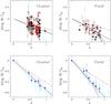 |
Fig. 17 The redshift evolution of the mass-to-light ratio for cluster (left) and field (right) galaxies. Top: black and red indicate galaxies with spectroscopic types 1 and 2, respectively. Morphologies for galaxies with HST photometry are coded as in Fig. 14. Galaxies with VLT photometry only are shown as crosses. Only galaxies with good VLT photometry (i.e., SExtractor flag 0 or 2) are plotted. The solid black lines show the solar metallicity SSP for zf = 2 (cluster) and zf = 1.2 (field). The solid red line shows the SSP for zf = 3.5 and half-solar metallicity, the cyan line shows the SSP for zf = 1.2 and twice-solar metallicity. The dotted line shows the best-fit linear relation (−0.55z for cluster and −0.76z for field galaxies) and the 1σ errors dashed. Bottom: the blue points show averages over redshift bins 0.1 wide. The cyan points are average field galaxies from van Dokkum & van der Marel (2007). Only field galaxies (plot to the right) with dynamical masses higher than 1011 M⊙ are considered. |
We compute dynamical masses as in Eq. (4). As discussed in the Introduction, the validity of this equation can be questioned in many respects. The value of the appropriate structural constant need not be the same for every galaxy. If ordered motions dominate the dynamics of a galaxy, as must be the case for disk galaxies, the use of velocity dispersion is inappropriate. Moreover, we also assume that the structure proportionality constant does not vary with redshift, which may not be true. Nevertheless, on average Eq. (4) delivers values that compare reasonably with stellar masses. We compute the (total) stellar masses from ground-based, rest-frame absolute photometry derived from SED fitting (Rudnick et al. 2009), adopting the calibrations of Bell & de Jong (2001), with a “diet” Salpeter IMF (with constant fractions of stars of mass less than 0.6 M⊙) and B − V colors, and renormalized using the corrections for an elliptical galaxy given in de Jong & Bell (2007). The method that calculates the rest-frame luminosities and colors is described in Rudnick et al. (2003), and the rest-frame filters were taken from Bessel (1990). Although the photometric redshifts and rest-frame SEDs were computed from the matched aperture photometry of White et al. (2005), the rest-frame luminosities were adjusted to total values, as described in Rudnick et al. (2009).
In general, the dynamical masses are somewhat lower than the stellar ones (Mdyn/M∗ = 0.91 for cluster galaxies, 0.75 for field galaxies), with an intrinsic scatter of a factor of two, on the order of the typical combined precision achieved for dynamical and stellar masses. If we consider only galaxies with HST morphology T < 0, the ratio Mdyn/M∗ drops to 0.74 for cluster and 0.56 for field galaxies. Moreover, a possible decreasing trend with redshift of the ratio Mdyn/M∗ is seen at the 2 − σ level, which is not unexpected given the size and velocity dispersion evolution discussed in Sect. 4.2. To conclude, the tendency for Mdyn/M∗ < 1 may indicate that the structural constant used in Eq. (4) is too low. However, we note that the structural constant is the one that dynamical studies at low redshifts prefer (Cappellari et al. 2006; Thomas et al. 2010). Alternatively, our adopted IMF contains too high a fraction of low mass stars (Baldry et al. 2008). Finally, we refer to Thomas et al. (2010) for a discussion of the role of dark matter in the estimation of Mdyn.
In the following, we consider relations as a function of both dynamical and stellar masses to assess the robustness of each result.
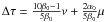
Figure 18 shows the residuals Δlog M/LB + 1.66log (1 + z) as a function of galaxy dynamical mass, for cluster (top) and field galaxies (bottom), at low (left) and high (right) redshifts. We divided the sample into three redshift bins of z < 0.5, 0.5 ≤ z < 0.7, and z ≥ 0.7. Averaging the points in mass bins 0.25 dex wide, one derives the following (see also Fig. 25). At low redshifts (z < 0.5), there is no convincing systematic trend between mass and residuals from the passively evolved FP, for both cluster (where the Pearson coefficient is 0.55 with a 2.5σ deviation from the no-correlation hypothesis) and field galaxies (where the Pearson coefficient is 0.15 for a t-value of 0.58 in agreement with the absence of a correlation). Within the errors, the solar metallicity SSP model with zf = 2 provides a reasonable description of the evolution of luminosity of all cluster and field early-type galaxies more massive than 1010 M⊙. At intermediate redshifts (0.5 ≤ z < 0.7), field (and to a lower extent cluster) galaxies with dynamical masses lower than 1011 M⊙ show systematically negative mean residuals. At higher redshifts (z ≥ 0.7), both cluster and field galaxies with masses lower than 1011 M⊙ show systematically negative mean residuals, i.e., are brighter than predicted by the passively evolved FP at zero redshift, with Spearman correlation coefficients between mass and residuals larger than 0.66 and a t-value of 6.3 for cluster galaxies. The trends are stronger if we restrict the sample to galaxies with HST early-type (T < 0) morphology. We note that down to masses ≈4 × 10¹⁰ M⊙ we sample a constant fraction (≈20%) of the existing galaxy population (see Fig. 13). At lower masses, however, this drops to just 10% and we can expect residual selection effects to play a role, as discussed in van der Wel et al. (2005). We do not detect any additional dependence on cluster velocity dispersion.
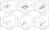 |
Fig. 18 The mass dependence of FP mass-to-light ratios. Top: the residuals Δlog M/LB + 1.66log (1 + z) as a function of galaxy mass for cluster galaxies at low (left, z < 0.5), intermediate (middle, 0.5 ≤ z < 0.7), and high (right, z > 0.7) redshift. The arrow in the top left panel shows the how points change due to the typical 10% error in velocity dispersion. Bottom: the residuals Δlog M/LB + 1.66log (1 + z) as a function of galaxy dynamical mass for field galaxies at low (left, z < 0.5), intermediate (middle, 0.5 ≤ z < 0.7), and high (right, z ≥ 0.7) redshift. Colors and symbols as in Fig. 17. The green points show averages over log Mdyn bins 0.25 dex wide. |
3.3. The rotation of the fundamental plane
As discussed by di Serego Alighieri et al. (2005), a mass dependence of the Δlog M/L residuals implies a rotation of the FP as a function of redshift. Here we investigate the effect by assuming that the zero-point variation Δlog M/LB = −1.66 × log (1 + z) for cluster and Δlog M/LB = −2.27 × log (1 + z) for field galaxies is caused entirely by pure luminosity evolution. Accordingly, we correct the surface brightnesses of cluster galaxies by applying the offset Δlog Ie = −1.66 × log (1 + z)/0.83 and of field galaxies by applying Δlog Ie = −2.27 × log (1 + z)/0.83. This agrees with the observed evolution of the average effective surface brightness (see dotted line in Fig. 10), except for the highest redshift bins. We then fit the parameters α and β of Eq. (1) using the maximum likelihood algorithm of Saglia et al. (2001), which uses multi-Gaussian functions to describe the distribution of data points, taking into account the full error covariance matrix and selection effects (for a Bayesian approach to the modeling of systematic effects, see Treu et al. 2001). To ensure conformity with the procedures adopted in the literature, the results were derived with and without taking into account selection effects, but the differences between the two approaches are always smaller than the large statistical errors. We analyzed three redshift ranges for cluster galaxies and two for field galaxies. The results are shown in Table 6. The errors were computed as the 68% percentile of the results of Monte Carlo simulations for each fitted sample as in Saglia et al. (2001). The low redshift bins (up to z = 0.7) infer α coefficients that are compatible with local values (α ≈ 1.2) and β coefficients (β ≈ 0.23−0.3) slightly smaller than the local value (β ≈ 0.33). In contrast, the highest redshift bins produce shallower log σ slopes. Given the relatively low number of galaxies per bin, especially in the low velocity dispersion regime, the statistical significance is just ≈1σ, but the trend confirms the claims of the literature (see Sect. 1). In particular, both values of α and β decrease at high redshift, as observed by di Serego Alighieri et al. (2005), a consequence of the flattening with redshift of the power-law relation between luminosity and mass (see Sect. 4).
The coefficients α and β of the EDisCS FP as a
function redshift and the derived quantities  (with
M/L ∝ Lϵ),
(with
M/L ∝ Lϵ),
 (with
L ∝ Mλ),
(with
L ∝ Mλ),
 .
.
4. Size and velocity dispersion evolution
4.1. Setting the stage
Up to this point, we have analyzed and interpreted the ZP variations of the FP based on the assumption that it is caused mainly by a variation in the luminosity. As discussed in the Introduction, there is growing evidence that early-type galaxies evolve not only in terms of luminosity, but also in size and velocity dispersion. Here we examine the consequences of these findings.
In general, if sizes were shrinking with increasing redshift, we would expect the surface
brightness to increase. Therefore, if the velocity dispersions do not increase a lot, the
net effect will be to reduce the net amount of brightening with redshift caused by stellar
population evolution. In detail, setting
ΔZP = ZP(z) − ZP(0)
and considering that  , we derive
  (6)where
 and
and
 are the
variations with redshifts in the mean half-luminosity radius and average surface
brightness. Therefore, the redshift variation in the luminosity, taking into account the
size and velocity dispersion evolution of galaxies is
are the
variations with redshifts in the mean half-luminosity radius and average surface
brightness. Therefore, the redshift variation in the luminosity, taking into account the
size and velocity dispersion evolution of galaxies is  (7)We note that the ZP
variations were determined by assuming constant α0 and
β0 coefficients, which is probably not true at the high
redshift end of our sample (see Sect. 3.3).
(7)We note that the ZP
variations were determined by assuming constant α0 and
β0 coefficients, which is probably not true at the high
redshift end of our sample (see Sect. 3.3).
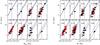 |
Fig. 19 The evolution in the Re − mass relation with redshift. Left: dynamical masses. Right: stellar masses. Colors and symbols are as in Fig. 17. The numbers give the average redshift in each bin. The full lines show the best-fit relation Re = Rc(M/2 × 1011 M⊙)0.56 with uniform galaxy weighting, the dashed lines with selection weighting. The blue lines show the reference line at zero redshifts. The vertical lines show the 2 × 10¹¹ M⊙ mass. |
The redshift evolution of the mass correlation fits.
If the variations are computed at constant dynamical mass, then
Δlog σ = −Δlog Re/2,
as in the “puffing” scenario of Fan et al. (2008, see
below) and Eq. (7) becomes
 (8)In this case, the
contribution of the size evolution to the luminosity evolution at constant mass derived
from the FP is zero if
(8)In this case, the
contribution of the size evolution to the luminosity evolution at constant mass derived
from the FP is zero if  (9)is zero, i.e.,
α0 = 10β0 −2. This is the
expected relation between α and β if the mass-to-light
ratio M/L varies as a power law of
the luminosity
M/L ∝ Lϵ,
in which case one has
(9)is zero, i.e.,
α0 = 10β0 −2. This is the
expected relation between α and β if the mass-to-light
ratio M/L varies as a power law of
the luminosity
M/L ∝ Lϵ,
in which case one has  ,
,  , and
, and
 .
Table 6 lists the values of ϵ,
λ, and A implied by the fits of the FP coefficients
performed in Sect. 3.3.
.
Table 6 lists the values of ϵ,
λ, and A implied by the fits of the FP coefficients
performed in Sect. 3.3.
If we parametrize all variations as a function of log (1 + z) as
Δlog Re = νlog (1 + z),
Δlog σ = μlog (1 + z), and
ΔZP = κlog (1 + z), we find that
 (10)where
φz is the correction for progenitor bias estimated by van Dokkum & Franx (2001) to be
φ = + 0.09. Their result can be applied to our work directly, since
our redshift dependence of the FP ZP closely matches that considered there.
(10)where
φz is the correction for progenitor bias estimated by van Dokkum & Franx (2001) to be
φ = + 0.09. Their result can be applied to our work directly, since
our redshift dependence of the FP ZP closely matches that considered there.
As discussed in the Introduction, the size and σ evolution of galaxies
is usually interpreted as a result of the merging history of galaxies. The merger models
of Hopkins et al. (2009) predict
νme ≈ −0.5 and μme = 0.1 for
galaxies with constant stellar mass M∗ ≈ 1011
with
(Mhalo/Rhalo)/(M∗/Re) ≈ 2.
This means that Δlog Re = −0.2Δlog σ. As an
alternative explanation, Fan et al. (2008) proposed
the “puffing” scenario, where galaxies grow in size conserving their mass as a result of
quasar activity. In this case, one has  . We note, however,
that this mechanism should already have come to an end at redshift 0.8. Moreover, the
strong velocity dispersion evolution predicted by the puffing scenario at redshifts higher
than 1 was ruled out by Cenarro & Trujillo
(2009).
. We note, however,
that this mechanism should already have come to an end at redshift 0.8. Moreover, the
strong velocity dispersion evolution predicted by the puffing scenario at redshifts higher
than 1 was ruled out by Cenarro & Trujillo
(2009).
Using ν = −0.5, μ = + 0.1, the change in the slope
 of the luminosity
evolution Δlog L = τlog (1 + z) (see
Eq. (7)) is ≈−0.5 units. We now
attempt to determine the values of ν and μ implied by
our dataset.
of the luminosity
evolution Δlog L = τlog (1 + z) (see
Eq. (7)) is ≈−0.5 units. We now
attempt to determine the values of ν and μ implied by
our dataset.
4.2. The redshift evolution of Re and σ
Following van der Wel et al. (2008), we investigated the size evolution of EDisCS galaxies by considering the Mass − Re relation for objects with masses higher that 3 × 10¹⁰ M⊙. In Fig. 19, we divided our sample into 8 redshift bins (centered on redshifts from 0.25 to 0.95 of bin size Δz = 0.1) and fit the relation Re = Rc(M/Mc)b. We considered both dynamical (Mdyn, left) and stellar (M∗, right) masses, and we weighted each galaxy with 1/PS. Within the errors, b does not vary much and is compatible with the values b = 0.56 found locally. In Fig. 19, we therefore keep its value fixed and determine Rc at the mass Mc = 2 × 10¹¹ M⊙. We fitted the function Rc(z) = Rc(0) × (1 + z)ν and summarize the values of the parameters resulting from the fits in Table 7. As becomes clear below, this does not necessarily describe the size evolution of a galaxy of fixed mass, but rather at any given redshift the mean value of the size of the evolving population of galaxies with this given mass.
Given the larger uncertainties in the Re values derived from VLT photometry, we first fitted the HST dataset alone (entries 1 and 2 of Table 7). Within the errors, both Rc(0) and the slope are very similar to the values reported by van der Wel et al. (2008, Rc(0.06) = 4.8 kpc, ν = 0.98 ± 0.11 for both dynamical and stellar mass fits. Our results do not change within the errors if we separately fit galaxies belonging to clusters or to the field. If we add the galaxies with VLT photometry only (entries 3 and 4 of Table 7), we derive larger Rc and steeper slopes.
Figure 20 shows Rc as a
function of redshift when we apply a correction for progenitor bias as in Valentinuzzi et al. (2010a). The EDisCS galaxies
considered here are a sample of spectroscopically selected passive objects. In contrast, a
morphologically selected local sample of early-type galaxies contains objects with
relatively young ages that, when evolved to EDisCS redshifts, would not be recognized as
being spectroscopically passive. Valentinuzzi et al.
(2010a) analyze the WINGS sample of local galaxies and determine their ages by
means of a spectral analysis. They select objects that were already passive (i.e., have an
age ≥1.5 Gyr) at the cosmic time of the redshifts
z = 0,0.25,0.5,0.75
and 1, and compute the median half-luminosity radii of massive galaxies. The resulting
Re vary as
Re = (4.1 ± 0.1) − (0.8 ± 0.2)z (kpc), when
selecting galaxies with dynamical masses
1011 < Mdyn/M⊙ < 3 × 10¹¹,
and as (4.3 ± 0.1) − (0.9 ± 0.2)z when selecting galaxies with stellar
masses
1011 < M∗/M⊙ < 3 × 10¹¹.
Therefore, we multiply the Rc(z) derived at
Mdyn = 1011M⊙ by
 , and those
at M∗ = 1011M⊙ by
, and those
at M∗ = 1011M⊙ by
 . With
these corrections, the residual evolution is small, and even compatible with no evolution
up to redshift z ≈ 0.7 with dynamical masses, and 0.5 with stellar
masses. Similar results are derived if we also consider the galaxies with VLT photometry,
with the caveats discussed above. Our correction for progenitor bias is of course somewhat
model-dependent, since objects might cross the boundaries between populations. For
example, there might be z ~ 0.6 passive galaxies that produce
z = 0 descendants with some younger stars, after accreting gas or
gas-rich objects.
. With
these corrections, the residual evolution is small, and even compatible with no evolution
up to redshift z ≈ 0.7 with dynamical masses, and 0.5 with stellar
masses. Similar results are derived if we also consider the galaxies with VLT photometry,
with the caveats discussed above. Our correction for progenitor bias is of course somewhat
model-dependent, since objects might cross the boundaries between populations. For
example, there might be z ~ 0.6 passive galaxies that produce
z = 0 descendants with some younger stars, after accreting gas or
gas-rich objects.
 |
Fig. 20 The size evolution with redshift of EDisCS galaxies corrected for progenitor bias
(see text). Left: Rc as a function of
redshift at 2 × 10¹¹M⊙ (see Fig. 19, left) derived using
Mdyn. Right:
Rc at
2 × 10¹¹ M⊙ (see Fig. 19, right) as a function of redshift derived using
M∗. The full lines show the best-fit function to the
galaxies with HST photometry (yellow points) |
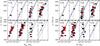 |
Fig. 21 The evolution of the σ-mass relation with redshift. Left: dynamical masses. Right: stellar masses. Colors and symbols as in Fig. 17. The numbers give the average redshift in each bin. The full lines show the best-fit relation σ = σC(M/MC)0.23 with uniform galaxy weighting, the dashed line with selection weighting. The blue lines show the reference line at zero redshifts. The vertical line indicates the MC = 2 × 10¹¹ M⊙ mass. |
In Figs. 21 and 22, we show the analogous plots and fits for the velocity dispersion.
Table 7 lists the relative results. We find that
σ scales as ≈ . The
trend weakens at low masses and high redshifts, especially when stellar masses are
considered. The fit at constant dynamical mass is just a consistency check, which should
infer a slope of the redshift dependence of opposite sign to and half the value of the one
measured for Rc (μ = +0.68) and this is the
case. In contrast, a weaker redshift evolution (μ = 0.39) is derived if
stellar masses are considered, in agreement with Cenarro
& Trujillo (2009). This is expected, since, as discussed above,
σc at fixed M∗ should
certainly be smaller than σc at fixed
Mdyn given that
Mdyn/M∗ < 1.
. The
trend weakens at low masses and high redshifts, especially when stellar masses are
considered. The fit at constant dynamical mass is just a consistency check, which should
infer a slope of the redshift dependence of opposite sign to and half the value of the one
measured for Rc (μ = +0.68) and this is the
case. In contrast, a weaker redshift evolution (μ = 0.39) is derived if
stellar masses are considered, in agreement with Cenarro
& Trujillo (2009). This is expected, since, as discussed above,
σc at fixed M∗ should
certainly be smaller than σc at fixed
Mdyn given that
Mdyn/M∗ < 1.
Following the procedure of Valentinuzzi et al.
(2010a) described above, we construct the local sample of WINGS galaxies with
velocity dispersions, trimmed to contain only massive spectroscopically passive galaxies
at the redshifts z = 0, 0.25, 0.5, 0.75, and 1, and compute the median
σ of massive galaxies. The resulting σ vary as
σ = (197 ± 2) + (6 ± 4)z km s-1, when
selecting galaxies with dynamical masses
1011 < Mdyn/M⊙ < 3 × 10¹¹,
and is constant at (210 ± 1.5) km s-1 when selecting galaxies with stellar
masses
1011 < M∗/M⊙ < 3 × 10¹¹.
Therefore, we correct the measured σc for the progenitor bias
by multiplying the values derived at
Mdyn = 1011M⊙ by
 , and no
correction is applied at constant stellar mass. The residual redshift evolution after the
correction and fitting the point at zero redshift is small.
, and no
correction is applied at constant stellar mass. The residual redshift evolution after the
correction and fitting the point at zero redshift is small.
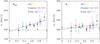 |
Fig. 22 The σ evolution with redshift of EDisCS galaxies corrected for
progenitor bias (see text). Left: σc as
a function of redshift derived using Mdyn.
Right: σc as a function of redshift
derived using M∗. The full lines show the best-fit
function |

Table 9 lists the changes in the slope
of the luminosity
evolution Δlog L = τlog (1 + z) (see
Eq. (7)) derived from the measured
variation in the FP ZP caused by the size and velocity dispersion evolution, coding the
different cases listed in Table 7. For example,
“case 1+9 Mdyn” uses the value of ν derived
for the redshift evolution of Rc constructed using the
Re − Mdyn relation with HST
data, without both selection weighting and progenitor bias correction (case 1 of
Table 7), and the value of μ
derived from the redshift evolution of σ inferred in turn from the
σ − Mdyn relation, without both selection
weighting and progenitor bias correction (case 9 of Table 7), obtaining Δτ = −0.39. This implies that the luminosity
evolution inferred from the ZP evolution of the EDisCS clusters without selection
weighting (L ~ (1 + z)1.61, see Table 5) reduces to
L ~ (1 + z)1.22.
The ages derived from the evolution of the FP ZP, averaged for Mdyn < 1011 M⊙ and Mdyn > 1011 M⊙.
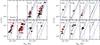 |
Fig. 23 The evolution of the luminosity-mass relation with redshift for cluster (left) and field (right) galaxies. Colors and symbols as in Fig. 17. The numbers give the average redshift in each bin. The full lines show the best-fit relation LB = Lc(M/MC)0.75, and the dotted lines L = Lc(M/MC)0.5, both relations having uniform galaxy weighting. The dashed lines show the 0.75 power law with selection weighting. The blue lines show the reference line at zero redshifts. The vertical line indicates the MC = 2 × 10¹¹ M⊙ mass. |
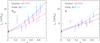 |
Fig. 24 The luminosity evolution with redshift of EDisCS galaxies. Left:
Lc as a function of redshift derived using
Mdyn. Right:
Lc as a function of redshift derived using
M∗. The full lines show the best-fit function
|

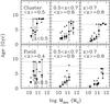 |
Fig. 25 The ages of cluster (top) and field (bottom) galaxies at low (left, z < 0.5 left), medium (0.5 < z < 0.7, middle), and high (z > 0.7, right) redshifts as a function of dynamical mass. The circles show the ages as derived from the bare FP zero-point evolution. The triangles pointing upwards take into account size evolution at constant M∗, case 3+7 (see Table 9). The triangles pointing downwards take into account the progenitor bias of van Dokkum & Franx (2001). The median redshifts are given and the corresponding ages of the universe are shown by the dotted lines. |
4.3. Luminosity evolution: the direct fit
To close the loop, in Fig. 23 we directly considered the relation between total luminosity LB and dynamical mass as a function of redshift. In general, the power law L = LC(M/MC)0.75 provides a reasonable fit to the data. Without selection weighting, we derived LC as a function of redshift as shown in Fig. 24 for dynamical and stellar masses. Fitting the power-law relation LC = LC(0)(1 + z)τ to z > 0.4 data points, separately for cluster and field galaxies, we derived the results listed in Table 7. The zero-redshift extrapolations compare well to the local values derived by considering the sample of Faber et al. (1989) (LC = 2.2 × 10¹⁰ L⊙ and M/LB = 8.9 M⊙/L⊙). As for the σc − z relation, we inferred a shallower luminosity evolution when measuring Lc at constant M∗. The luminosity evolution with redshift is steeper for field galaxies.
Given the large errors in the luminosity fits, the derived luminosity evolution agrees with the ones derived from the FP analysis. At face value, the FP ZPs without size and velocity dispersion evolution corrections slightly overestimate the luminosity evolution at constant stellar mass and underestimate that at constant dynamical mass. This corroborates the conclusion that the corrections Δτ for size and velocity dispersion evolution must be small, as one finds when the progenitor bias is taken into account.
4.4. Ages
As a final step, we translated the observed evolution in the FP zero points, into an age estimate. We examined three cases that define the realistic range of possible luminosity evolutions: (1) minimal evolution, using Δτ = −0.7 (M∗, case 6+12, of Table 7) and φ = 0; (2) Δτ = 0 and φ = 0, where the small size and velocity dispersion correction compensates the progenitor bias of van Dokkum & Franx (2001); (c) Δlog L = φz, where the size and velocity dispersion correction is zero and we take into account the progenitor bias of van Dokkum & Franx (2001). We convert the mean Δlog M/LB for cluster and field galaxies measured in the mass bins of Fig. 18 into an age, by considering the various options for size evolution discussed above. We use the solar-metallicity (motivated by the analysis of the averaged line indices discussed below), Salpeter IMF SSP models of Maraston (2005) at the appropriate mean redshift of the bin. Ages older than the age of the universe at that redshift are set to the age of the universe. Figure 25 shows the results, Table 8 gives the average values for Mdyn < 1011 M⊙ and Mdyn > 1011 M⊙.
Field galaxies are slightly younger than cluster galaxies at the same redshift and mass. Taking into account the size and velocity dispersion evolution considered above in the case 6+12 pushes all formation ages upwards by 1−4 Gyr. Taking into account the progenitor bias of van Dokkum & Franx (2001) reduces the ages by 1−2 Gyr. Table 8 lists the mean ages of the HST sample of galaxies with morphologies T < 0. The differences between low and high mass galaxies are smaller.
We next correlated the FP ages of Fig. 25 with those derived from the analysis of the spectral indices. As performed in Sánchez-Blázquez et al. (2009), we averaged the spectra of the galaxies appearing in each mass bin shown in Fig. 18, measured the Fe4383, HdA, and CN2 indices, and recovered the ages and metallicities of SSP models that reproduce their values best. The derived metallicity averaged over the sample is solar, which justifies the choice above. We also estimated luminosity-weighted and mass-weighted ages directly by fitting the spectra with a library of model spectra. Within the large errors, there is overall agreement with the ages derived from the indices. The optimal match is achieved when considering the minimal evolution ages. As a final check, we evaluated the rest-frame U − B and B − V colors corresponding to a SSP of solar metallicity and age derived above and compared them to the measured averaged colors. The agreement was fair, but either the colors predicted using the FP ages are too red or the spectral ages appear to be too high. The discrepancy is exacerbated when size evolution is taken into account. This could simply reflect the known difficulties for stellar population synthesis models in reproducing the colors of real galaxies (Maraston et al. 2009).
5. Conclusions
We have examined the FP of EDisCS spectroscopic early-type galaxies, in both the cluster and the field. Combining structural parameters from HST and VLT images and velocity dispersions from VLT spectra, we have compiled a catalogue of 154 cluster and 68 field objects in the redshift range 0.2−0.9. For the first time, we have explored the FP of galaxy clusters of medium-to-low velocity dispersion in the redshift range 0.4−0.9. At face-value, on average, the evolution of the zero point follows the predictions of simple stellar population models with high (≈2) formation redshift for all clusters, independent of their velocity dispersion, with a slight increase (from 15% to 18%) in the scatter in mass-to-light ratios for clusters with low (σclus < 600 km s-1) velocity dispersions. The FP zero point of field galaxies follows similar tracks up to redshift ≈0.5, but implies brighter luminosities, or lower formation redshifts at higher redshifts.
We have determined dynamical and stellar masses for our galaxies. The ratio Mdyn/M∗ is ≈0.9 with a scatter of a factor of 2 and a tendency to decrease with redshift. We investigated the FP residuals as a function of galaxy mass. At high redshifts (z > 0.7 for cluster galaxies, slightly below for field galaxies), galaxies with mass lower than ≈1011 M⊙ have lower mass-to-light ratios than a passive evolution of the ZP predicts. This implies that there is a rotation in the FP: we have confirmed that for cluster galaxies the velocity dispersion coefficient α is compatible with the local value up to a redshift z = 0.7 and decreases to α ≈ 0.7 ± 0.4 at higher redshifts, but this detection is of low statistical significance.
We have investigated the size and velocity dispersion evolution of our sample. At a given mass, galaxy sizes decrease and velocity dispersions increase at increasing redshift. We fitted the relations Re ≈ (1 + z) − 1.0 ± 0.3, and σ ≈ (1 + z)0.59 ± 0.1 and σ ≈ (1 + z)0.34 ± 0.14 at a constant dynamical or stellar mass of 2 × 10¹¹ M⊙, respectively, for both cluster and field galaxies. However, after taking into account the progenitor bias affecting our sample (large galaxies that joined the local early-type class only recently will progressively disappear in higher redshift samples), the effective size and velocity dispersion evolution reduced substantially (to Re ∝ (1 + z) − 0.5 ± 0.2 and σ ∝ (1 + z)0.41 ± 0.08 for dynamical masses and Re ∝ (1 + z) − 0.68 ± 0.4 and σ ∝ (1 + z)0.19 ± 0.10 for stellar masses).
We computed the luminosity evolution predicted by the ZP variation with redshift of the FP when the size and velocity dispersion evolution are taken into account. The corrections computed at constant dynamical masses with a progenitor bias correction almost cancel out; at constant stellar mass, they reduce the slope of the (1 + z) dependence of luminosity by −0.6 units (case 5+11 of Table 7). Fitting directly the luminosity-mass relation, we derived a luminosity evolution that agrees with the one derived from the FP analysis and does not allow for large size and velocity dispersion corrections such as those derived without taking into account the progenitor bias, where a reduction of the slope of the (1 + z) dependence of luminosity by −0.8 is derived at constant M∗ (case 1+9 of Table 7).
Using SSP models, we translated the variations in the FP ZP into formation ages as a function of redshift and galaxy mass. Massive (M > 1011 M⊙) cluster galaxies are old, with formation redshifts zf > 1.5. In contrast, lower mass galaxies are just 2 to 3 Gyr old. This agrees with the EDisCS results presented in De Lucia et al. (2004, 2007), Poggianti et al. (2006), Sánchez-Blázquez et al. (2009), and Rudnick et al. (2009), who argue from different points of view that the lower luminosity, lower mass population of early-type galaxies comes in place only at later stages in clusters. Field galaxies at all masses are somewhat younger (by ≈1 Gyr) than the cluster ones with similar masses and redshifts. In general, the FP ages agree reasonably well with those derived from spectral indices.
To conclude, our analysis of the FP, size, and velocity dispersion evolution of EDisCS galaxies points towards a picture where a large fraction of the population became passive only fairly recently. The high-redshift passive galaxies are a biased subset of all present-day passive galaxies. At any probed redshift, from 0 to 1, passive galaxies are an inhomogeneous population in terms of their formation paths, and as redshift increases, a subset of the population leaves the sample, with the less massive galaxies dropping out of the sample more rapidly with redshift than the more massive ones, and at a somewhat accelerated rate in the field. Only when these effects are taken into account may coherent estimates of the luminosity evolution of early-type galaxies from the colors, indices, and the FP zero point be derived.
Online material
6. table
The FP parameters of cluster galaxies.
The FP parameters of field galaxies.
The structural parameters of galaxies with measured velocity dispersions and HST photometry derived from Sersic fits to HST images and bulge+disk fits to VLT images.
Appendix A: Circularized half-luminosity radii
GIM2D delivers bulge ae and disk
ah scale lengths along the major axis,
bulge apparent flattening
(b/a)B
and disk inclination angles i (corresponding to an apparent flattening
(b/a)D = 1 − cosi),
and bulge-to-total ratios B/T. When
fitting Sersic profiles, GIM2D delivers the n Sersic index, the major
axis  , and
the flattening (b/a)Ser.
We compute the circularized half-luminosity radius Re of the
resulting galaxy model as follows. We determine the flux inside a circular aperture of
radius R (the so-called curve of growth) of a model of apparent
flattening b/a and surface density
distribution constant on ellipses
, and
the flattening (b/a)Ser.
We compute the circularized half-luminosity radius Re of the
resulting galaxy model as follows. We determine the flux inside a circular aperture of
radius R (the so-called curve of growth) of a model of apparent
flattening b/a and surface density
distribution constant on ellipses  as
as  (A.1)Using
 , we derive
 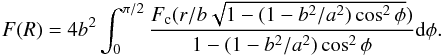 (A.2)We perform the
angular integration numerically, using
(A.2)We perform the
angular integration numerically, using 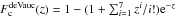 , where
z = 7.67(r/ReB)1/4,
and
, where
z = 7.67(r/ReB)1/4,
and 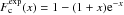 , and
x = R/h for the
normalized de Vaucouleurs and exponential density laws, respectively. For a Sersic
profile of given n, we use
, and
x = R/h for the
normalized de Vaucouleurs and exponential density laws, respectively. For a Sersic
profile of given n, we use  , where
P is the incomplete Γ function and
X = k(r/ReSer)1/n
and k = 1.9992n − 0.3271 (Simard et al. 2002). We determine Re by
solving the equation
, where
P is the incomplete Γ function and
X = k(r/ReSer)1/n
and k = 1.9992n − 0.3271 (Simard et al. 2002). We determine Re by
solving the equation  (A.3)for the
bulge-plus-disk models, and
(A.3)for the
bulge-plus-disk models, and 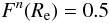 (A.4)for the
Sersic fits numerically. In general, the resulting Re agree
within 1% with the half-luminosity radii derived by measuring the curves of growth
directly from (ACS HST like) images generated by GIM2D with the fit parameters and no
PSF convolution, but the image-based method overestimates Re
by up to 10% when it is smaller than 4 pixels (0.2 arcsec).
(A.4)for the
Sersic fits numerically. In general, the resulting Re agree
within 1% with the half-luminosity radii derived by measuring the curves of growth
directly from (ACS HST like) images generated by GIM2D with the fit parameters and no
PSF convolution, but the image-based method overestimates Re
by up to 10% when it is smaller than 4 pixels (0.2 arcsec).
Figure A.1 illustrates that a more accurate
approximation of the circularized radius Re(Ser) of Sersic
profiles, more accurate than 2%, is obtained by taking the simple mean
Rave = (ae + be)/2
of the major and minor axis scale lengths ae and
be instead of the harmonic mean  .
This is surprising only at a first sight, since Rhar goes to
zero as the flattening increases, while Rave does not.
Therefore Rave should provide a closer approximation of the
half-luminosity radius derived from circular curves of growth at high ellipticities. On
the other hand, the effective surface brightness within the ellipse of semi-major and
minor axis ae and be is constant
regardless of the flattening, while this is not true for the surface brightness within
the circle of radius Re(Ser). Since in this exercise the
total luminosity L is kept constant, we have
.
This is surprising only at a first sight, since Rhar goes to
zero as the flattening increases, while Rave does not.
Therefore Rave should provide a closer approximation of the
half-luminosity radius derived from circular curves of growth at high ellipticities. On
the other hand, the effective surface brightness within the ellipse of semi-major and
minor axis ae and be is constant
regardless of the flattening, while this is not true for the surface brightness within
the circle of radius Re(Ser). Since in this exercise the
total luminosity L is kept constant, we have  , with
  and
and  .
This is almost orthogonal to the FP (see Eq. (1)), making the choice of method unimportant, as long as not too many disks
seen edge-one (i.e. of very high flattening) are present in the sample (see Fig. 5 and discussion in Sect. 2.2).
.
This is almost orthogonal to the FP (see Eq. (1)), making the choice of method unimportant, as long as not too many disks
seen edge-one (i.e. of very high flattening) are present in the sample (see Fig. 5 and discussion in Sect. 2.2).
 |
Fig. A.1 The circularized half-luminosity radius Re(Ser) of
the sample of EDisCS galaxies with HST photometry and velocity dispersions
computed according to Eqs. (A.2)
and (A.4) compared to the simple
mean
Rave = 0.5(ae + be)
(top) and harmonic mean |
Acknowledgments
This work was supported by the Sonderforschungsbereich 375 of the German Research Foundation. The Dark Cosmology Centre is funded by the Danish National Research Foundation. GDL acknowledges financial support from the European Research Council under the European Community’s Seventh Framework Programme (FP7/2007-2013)/ERC grant agreement n. 202781. The anonymous referee report helped us improve the presentation of the results.
References
- Baldry, I. K., Glazerbrook, K., & Driver, S. P. 2008, MNRAS, 388, 945 [NASA ADS] [Google Scholar]
- Bell, E. F., & de Jong, R. S. 2001, ApJ, 550, 21 [NASA ADS] [CrossRef] [Google Scholar]
- Bender, R., Saglia, R. P., & Gerhard, O. 1994, MNRAS, 269, 785 [NASA ADS] [CrossRef] [Google Scholar]
- Bender, R., Saglia, R. P., Ziegler, B., et al. 1998, ApJ, 493, 529 [NASA ADS] [CrossRef] [Google Scholar]
- Bertin, E., & Arnouts, S. 1996, A&AS, 117, 393 [NASA ADS] [CrossRef] [EDP Sciences] [Google Scholar]
- Bessel, M. S. 2990, PASP, 102, 1181 [Google Scholar]
- Biermann, P., & Shapiro, S. L. 1979, ApJ, 230, L33 [NASA ADS] [CrossRef] [Google Scholar]
- Blakeslee, J. P., Franx, M., Postman, M., et al. 2003, ApJ, 596, L143 [NASA ADS] [CrossRef] [Google Scholar]
- Bruzual, G., & Charlot, S. 2003, MNRAS, 344, 1000 [NASA ADS] [CrossRef] [Google Scholar]
- Burstein, D., Davies, R. L., Dressler, A., et al. 1987, ApJS, 64, 601 [NASA ADS] [CrossRef] [Google Scholar]
- Buitrago, F., Trujillo, I., Conselice, C. J., et al. 2008, ApJ, 687, L61 [NASA ADS] [CrossRef] [Google Scholar]
- Cappellari, M., & Emsellem, E. 2004, PASP, 116, 138 [NASA ADS] [CrossRef] [Google Scholar]
- Cappellari, M., Bacon, R., Bureau, M., et al. 2006, MNRAS, 366, 1126 [NASA ADS] [CrossRef] [Google Scholar]
- Cappellari, M., di Serego Alighieri, S., Cimatti, A., et al. 2009, ApJ, 704, L34 [NASA ADS] [CrossRef] [Google Scholar]
- Carlberg, R. G., Yee, H. K. C., Ellingson, E., et al. 1996, ApJ, 462, 32 [Google Scholar]
- Cenarro, A. J., & Trujillo, I. 2009, ApJ, 696, L43 [NASA ADS] [CrossRef] [Google Scholar]
- Cimatti, A., Cassata, P., Pozzetti, L., et al. 2008, A&A, 482, 21 [NASA ADS] [CrossRef] [EDP Sciences] [Google Scholar]
- Clowe, D., Schneider, P., Aragón-Salamanca, A., et al. 2006, A&A, 451, 395 [NASA ADS] [CrossRef] [EDP Sciences] [Google Scholar]
- Colless, M., Saglia, R. P., Burstein, D., et al. 2001, MNRAS, 321, 277 [NASA ADS] [CrossRef] [Google Scholar]
- Conroy, C., & Gunn, J. E. 2010, ApJ, 712, 833 [NASA ADS] [CrossRef] [Google Scholar]
- Daddi, E., Renzini, A., Pirzkal, N., et al. 2005, ApJ, 626, 680 [NASA ADS] [CrossRef] [Google Scholar]
- Damjanov, I., McCarthy, P. J., Abraham, R. G., et al. 2009, ApJ, 695, 101 [NASA ADS] [CrossRef] [Google Scholar]
- de Jong, R. S., Simard, L., Davies, R. L., et al. 2004, MNRAS, 355, 1155 [NASA ADS] [CrossRef] [Google Scholar]
- de Jong, R. S., & Bell, E. F. 2007, ed. R. S. de Jong (Springer), ApS&S Proc., 107 [Google Scholar]
- De Lucia, G., Poggianti, B. M., Aragón-Salamanca, A., et al. 2004, ApJ, 610, L77 [NASA ADS] [CrossRef] [Google Scholar]
- De Lucia, G., Springel, V., White, S. D. M., Croton, D., & Kauffmann, G. 2006, MNRAS, 366, 499 [NASA ADS] [CrossRef] [Google Scholar]
- De Lucia, G., Poggianti, B. M., Aragón-Salamanca, A., et al. 2007, MNRAS, 374, 809 [NASA ADS] [CrossRef] [Google Scholar]
- Desai, V., Dalcanton, J. J., Aragón-Salamanca, A., et al. 2007, ApJ, 661, 1151 [NASA ADS] [CrossRef] [Google Scholar]
- Di Serego Alighieri, S., Vernet, J., et al. 2005, A&A, 442, 125 [NASA ADS] [CrossRef] [EDP Sciences] [Google Scholar]
- Di Serego Alighieri, S., Lanzoni, B., & Jørgensen, I. 2006, ApJ, 652, L145 [NASA ADS] [CrossRef] [Google Scholar]
- Djorgovski, S., & Davis, M. 1987, ApJ, 313, 59 [Google Scholar]
- D’Onofrio, M., Fasano, G., Varela, J., et al. 2008, ApJ, 685, 875 [NASA ADS] [CrossRef] [Google Scholar]
- Dressler, A., Faber, S. M., Burstein, D., et al. 1987, ApJ, 313, L37 [NASA ADS] [CrossRef] [Google Scholar]
- Dressler, A., Oemler, A., Jr., Couch, W. J., et al. 1997, ApJ, 490, 577 [NASA ADS] [CrossRef] [Google Scholar]
- Edwards, S., Colless, M., Bridges, T., et al. 2002, ApJ, 567, 178 [NASA ADS] [CrossRef] [Google Scholar]
- Faber, S. M., Wegner, G., Burstein, D., et al. 1989, ApJS, 69, 763 [NASA ADS] [CrossRef] [Google Scholar]
- Fan, L., Lapi, A., De Zotti, G., & Danese, L. 2008, ApJ, 689, L101 [NASA ADS] [CrossRef] [Google Scholar]
- Ferreras, I., Lisker, T., Pasquali, A., Khochfar, S., & Kavira, S. 2009, MNRAS, 395, 554 [NASA ADS] [CrossRef] [Google Scholar]
- Fisher, D., Fabricant, D., Franx, M., & van Dokkum, P. 1998, ApJ, 498, 195 [NASA ADS] [CrossRef] [Google Scholar]
- Gebhardt, K., Faber, S. M., Koo, D. C., et al. 2003, ApJ, 597, 239 [NASA ADS] [CrossRef] [Google Scholar]
- Gómez, P. L., Hughes, J. P., & Birkinshaw, M. 2000, ApJ, 540, 726 [NASA ADS] [CrossRef] [Google Scholar]
- Halliday, C., Milvang-Jensen, B., Poirer, S., et al. 2004, A&A, 427, 397 [NASA ADS] [CrossRef] [EDP Sciences] [Google Scholar]
- Hudson, M. J., Russell, J. S., Lucey, J. R., & Branchini, E. 2004, MNRAS, 352, 61 [Google Scholar]
- Holden, B. P., van der Wel, A., Franx, M., et al. 2005, ApJ, 620, L83 [NASA ADS] [CrossRef] [Google Scholar]
- Hopkins, P. F., Hernquist, L., Cox, T. J., Keres, D., & Wuyts, S. 2009, ApJ, 691, 1424 [NASA ADS] [CrossRef] [Google Scholar]
- Jaffé, Y. L., Aragón-Salamanca, A., De Lucia, G., et al. 2010, MNRAS, in press [Google Scholar]
- Johnson, O., Best, D., Zaritsky, D., et al. 2006, MNRAS, 371, 1777 [NASA ADS] [CrossRef] [Google Scholar]
- Jørgensen, I., Franx, M., & Kjaergaard, P. 1995, MNRAS, 276, 1341 [NASA ADS] [Google Scholar]
- Jørgensen, I., Franx, M., Hjorth, J., & van Dokkum, P. G. 1999, MNRAS, 308, 833 [NASA ADS] [CrossRef] [Google Scholar]
- Jørgensen, I., Bergmann, M., Davies, R., et al. 2005, AJ, 129, 1249 [NASA ADS] [CrossRef] [Google Scholar]
- Jørgensen, I., Chiboucas, K., Flint, K., et al. 2006, ApJ, 639, L9 [NASA ADS] [CrossRef] [Google Scholar]
- Jørgensen, I., Chiboucas, K., Flint, K., et al. 2007, ApJ, 654, L179 [NASA ADS] [CrossRef] [Google Scholar]
- Just, D. W., Zaritsky, D., Sand, D. J., Desai, V., & Rudnick, G. 2010, ApJ, 711, 192 [NASA ADS] [CrossRef] [Google Scholar]
- Kauffmann, G. 1996, MNRAS, 281, 475 [NASA ADS] [CrossRef] [Google Scholar]
- Kelson, D. D., Illingworth, G. D., van Dokkum, P. G., & Franx, M. 2000, ApJ, 531, 184 [NASA ADS] [CrossRef] [Google Scholar]
- Khochfar, S., & Silk, J. 2006, ApJ, 468, L21 [CrossRef] [Google Scholar]
- Kochanek, C. S., Falco, E. E., Impey, C. D., et al. 2000, ApJ, 543, 131 [NASA ADS] [CrossRef] [Google Scholar]
- Le Borgne, J. F., Pello, R., & Sanahuja, B. 1992, A&AS, 95, 87 [NASA ADS] [Google Scholar]
- Longhetti, M., Saracco, P., Severgnini, P., et al. 2007, MNRAS, 374, L614 [NASA ADS] [CrossRef] [Google Scholar]
- Lynden-Bell, D., Faber, S. M., Burstein, D., et al. 1988, ApJ, 326, 19 [NASA ADS] [CrossRef] [Google Scholar]
- Mancini, C., Daddi, E., Renzini, A., et al. 2010, MNRAS, 401, 933 [NASA ADS] [CrossRef] [Google Scholar]
- Maraston, C. 2005, MNRAS, 362, 799 [NASA ADS] [CrossRef] [Google Scholar]
- Maraston, C., Strömback, G., Thomas, D., Wake, D. A., & Nichol, R. C. 2009, MNRAS, 394, L107 [NASA ADS] [CrossRef] [Google Scholar]
- MacArthur, L. A., Ellis, R. S., Treu, T. U. V., Bundy, K., & Moran, S. 2008, ApJ, 680, 70 [NASA ADS] [CrossRef] [Google Scholar]
- Mellier, Y., Soucail, G., Fort, B., & Mathez, G. 1988, A&A, 199, 13 [NASA ADS] [Google Scholar]
- Milvang-Jensen, B., Noll, S., Halliday, C., et al. 2008, A&A, 482, 419 [NASA ADS] [CrossRef] [EDP Sciences] [Google Scholar]
- Menanteau, F., Ford, H. C., Illingworth, G. D., et al. 2004, ApJ, 612. 202 [NASA ADS] [CrossRef] [Google Scholar]
- Pelló, R., Rudnick, G., De Lucia, G., et al. 2009, A&A, 508, 1173 [NASA ADS] [CrossRef] [EDP Sciences] [Google Scholar]
- Pérez-González, P. G., Trujillo, I., Barro, G., et al. 2008, ApJ, 687, 50 [NASA ADS] [CrossRef] [Google Scholar]
- Poggianti, B. M., von der Linden, A., de Lucia, G., et al. 2006, ApJ, 642, 188 [NASA ADS] [CrossRef] [Google Scholar]
- Rudnick, G., et al. 2003, ApJ, 599, 487 [Google Scholar]
- Rudnick, G., von der Linden, A., Pelló, R., et al. 2009, ApJ, 700, 1559 [NASA ADS] [CrossRef] [Google Scholar]
- Saglia, R. P., Bertschinger, E., Baggley, G., et al. 1997a, ApJS, 109, 79 [NASA ADS] [CrossRef] [Google Scholar]
- Saglia, R. P., Burstein, D., Baggley, G., et al. 1997b, MNRAS, 292, 499 [NASA ADS] [Google Scholar]
- Saglia, R. P., Colless, M., Burstein, D. et al. 2001, MNRAS, 324, 389 [NASA ADS] [CrossRef] [Google Scholar]
- Saglia, R. P., Bender, R., & Dressler, A. 2003, A&A, 279, 75 [Google Scholar]
- Sánchez-Blázquez, P., Peletier, R. F., Jiménez-Vicente, J., et al. 2006, MNRAS, 371, 703 [NASA ADS] [CrossRef] [Google Scholar]
- Sánchez-Blázquez, P., Jablonka, P., Desai, V., et al. 2009, A&A, 499, 47 [NASA ADS] [CrossRef] [EDP Sciences] [Google Scholar]
- Saracco, P., Longhetti, M., & Andreon, S. 2009, MNRAS, 392, 718 [NASA ADS] [CrossRef] [Google Scholar]
- Shen, S., Mo, H. J., White, S. D. M., et al. 2003, MNRAS, 343, 978 [NASA ADS] [CrossRef] [Google Scholar]
- Simard, L., Willmer, C. N. A., Vogt, N. P., et al. 2002, ApJS, 142, 1 [NASA ADS] [CrossRef] [Google Scholar]
- Simard, L., Willmer, C. N. A., Vogt, N. P., et al. 2009, A&A, 508, 1141 [NASA ADS] [CrossRef] [EDP Sciences] [Google Scholar]
- Thomas, J., Saglia, R. P., Bender, R., et al. 2010, MNRAS, submitted [Google Scholar]
- Toft, S., van Dokkum, P., Franx, M., et al. 2007, ApJ, 671, 285 [NASA ADS] [CrossRef] [MathSciNet] [Google Scholar]
- Tran, K.-V., van Dokkum, P., Illingworth, G. D., et al. 2005, ApJ, 619, 134 [NASA ADS] [CrossRef] [Google Scholar]
- Treu, T., Stiavelli, M., Bertin, G., Casertano, S., & Møller, P. 2001, MNRAS, 326, 237 [NASA ADS] [CrossRef] [Google Scholar]
- Treu, T., Stiavelli, M., Casertano, S., Møller, P., & Bertin, G. 2002, ApJ, 564, L13 [NASA ADS] [CrossRef] [Google Scholar]
- Treu, T., Ellis, R. S., Liao, T. X., et al. 2005a, ApJ, 633, 174 [NASA ADS] [CrossRef] [Google Scholar]
- Treu, T., Ellis, R. S., Liao, T. X., & van Dokkum, P. G. 2005b, ApJ, 622, L5 [NASA ADS] [CrossRef] [Google Scholar]
- Trujillo, I., Förster Schreiber, N. M., Rudnick, G., et al. 2006, ApJ, 650, 18 [NASA ADS] [CrossRef] [Google Scholar]
- Trujillo, I., Conselice, C. J., Bundy, K., et al. 2007, MNRAS, 382, 109 [NASA ADS] [CrossRef] [Google Scholar]
- Valentinuzzi, T., Fritz, J., Poggianti, B. M., et al. 2010a, ApJ, 712, 226 [NASA ADS] [CrossRef] [Google Scholar]
- Valentinuzzi, T., Poggianti, B. M., Saglia, R. P., et al. 2010b, ApJ, 721, L19 [NASA ADS] [CrossRef] [Google Scholar]
- van der Marel, R., & van Dokkum, P. G. 2007a, ApJ, 668, 738 [NASA ADS] [CrossRef] [Google Scholar]
- van der Marel, R., & van Dokkum, P. G. 2007b, ApJ, 668, 756 [NASA ADS] [CrossRef] [Google Scholar]
- van der Wel, A., Franx, M., van Dokkum, P. G., & Rix, H.-W. 2004, ApJ, 601, L5 [NASA ADS] [CrossRef] [Google Scholar]
- van der Wel, A., Franx, M., van Dokkum, P. G., et al. 2005, ApJ, 631, 145 [NASA ADS] [CrossRef] [Google Scholar]
- van der Wel, A., Holden, B. P., Zirm, A. W., et al. 2008, ApJ, 688, 48 [NASA ADS] [CrossRef] [Google Scholar]
- van Dokkum, P. G., & Franx, M. 1996, MNRAS, 281, 985 [NASA ADS] [CrossRef] [Google Scholar]
- van Dokkum, P. G., & Franx, M. 2001, ApJ, 553, 90 [Google Scholar]
- van Dokkum, P. G., & Stanford S. A. 2003, ApJ, 585, 78 [NASA ADS] [CrossRef] [Google Scholar]
- van Dokkum, P. G., & van der Marel, R. 2007, ApJ, 655, 30 [NASA ADS] [CrossRef] [Google Scholar]
- van Dokkum, P. G., Franx, M., Kelson, D. D., & Illingworth, G. D. 1998, ApJ, 504, L17 [NASA ADS] [CrossRef] [Google Scholar]
- van Dokkum, P. G., Franx, M., Fabricant, D., et al. 2000, ApJ, 541, 95 [NASA ADS] [CrossRef] [Google Scholar]
- van Dokkum, P. G., Franx, M., Kelson, D. D., & Illingworth, G. D. 2001, ApJ, 553, L39 [NASA ADS] [CrossRef] [Google Scholar]
- van Dokkum, P. G., Franx, M., Kriek, M., et al. 2008, ApJ, 667, L5 [NASA ADS] [CrossRef] [Google Scholar]
- van Dokkum, P. G., Kriek, M., & Franx, M. 2009, Nature, 460, 717 [NASA ADS] [CrossRef] [PubMed] [Google Scholar]
- van Dokkum, P. G., Whitaker, K. E., Brammer, G., et al. 2010, ApJ, 709, 1018 [NASA ADS] [CrossRef] [Google Scholar]
- Vazdekis, A., Sánchez-Blázquez, P., Falcón-Barroso, J., et al. 2010, MNRAS, 404, 1639 [NASA ADS] [Google Scholar]
- White, S. D. M., Aragón-Salamanca, A., Bender, R., et al. 2005, A&A, 444, 365 [NASA ADS] [CrossRef] [EDP Sciences] [Google Scholar]
- Wuyts, S., van Dokkum, P. G., Kelson, D. D., Franx, M., & Illingworth, G. D. 2004, ApJ, 605, 677 [NASA ADS] [CrossRef] [Google Scholar]
- Zaritsky, D., Zabludoff, A. I., & Gonzalez, A. H. 2008, ApJ, 682, 68 [NASA ADS] [CrossRef] [Google Scholar]
- Ziegler, B. L., Thomas, D., Böhm, A., et al. 2005, A&A, 433, 519 [NASA ADS] [CrossRef] [EDP Sciences] [Google Scholar]
- Zirm, A. W., van der Wel, A., Franx, M., et al. 2007, ApJ, 656, 66 [NASA ADS] [CrossRef] [Google Scholar]
All Tables
The parameters of the EDisCS clusters with measured FP zero points Δlog M/LB, without selection weighting.
The slopes of the zero-point evolution of the FP Δlog M/L = 0.4(ZP(z) − ZP(0))/β0 = η′z = ηlog (1 + z).
The coefficients α and β of the EDisCS FP as a
function redshift and the derived quantities
(with
M/L ∝ Lϵ),
(with
L ∝ Mλ),
.
The ages derived from the evolution of the FP ZP, averaged for Mdyn < 1011 M⊙ and Mdyn > 1011 M⊙.
The structural parameters of galaxies with measured velocity dispersions and HST photometry derived from Sersic fits to HST images and bulge+disk fits to VLT images.
All Figures
|
Fig. 1 The velocity dispersion errors. First row: the histograms of statistical errors on velocity dispersions. Second row: the statistical errors as a function of apparent I band magnitude in a 1 arcsec radius aperture. Colors code the spectroscopic type (black: 1; red: 2). |
| In the text | |
|
Fig. 2 The histogram of the fractional aperture corrections σcor/σmes for cluster (left) and field (right) galaxies. |
| In the text | |
|
Fig. 3 The velocity dispersions of the galaxy sample. Top: the measured galaxy velocity dispersions as a function of redshift in clusters (left) and the field (right). The green lines show the mean values in 0.1 redshift bins and the relative errors. The dotted lines show the mean values weighting each galaxy with the inverse of its completeness value. Bottom: the histogram of galaxy velocity dispersions in clusters (left) and the field (right). Colors code the spectral type (black: 1; red:2). The dotted lines show the histogram for the entire sample irrespective of spectral type. |
| In the text | |
|
Fig. 4 The properties of the bulge+disk fits to galaxies with HST photometry and a measured velocity dispersion. We plot the ratio ae/Re of the semi-major effective scale length ae of the best-fit Sersic profile to the circularized effective radius Re of the best-fit B+D model (top), the bulge-to-total ratio B/T (middle), and the Sersic index nSer (bottom) as a function of the ellipticity 1 − be/ae (where be is the semi-minor effective scale length) of the Sersic fit. Objects with B/T > 0.5 are plotted in red, the remainder in blue. Symbols code the morphology: filled ellipses show T ≤ −4, filled circles crossed by a line −3 ≤ T ≤ 0, spirals T > 0. |
| In the text | |
|
Fig. 5 The comparison between different estimations of the half-luminosity radii of all galaxies with HST photometry and a measured velocity dispersion. We plot the ratio of the harmonic radius (aebe)1/2 to the circularized effective radius Re of the best-fit HST B+D model (top), the ratio of the circularized effective radius Re(Ser) of the Sersic fit to Re (middle), and the ratio of the circularized effective radius Re(VLT) of the best-fit VLT B+D model to Re (bottom) as a function of 1 − be/ae. Symbols and color coding are as in Fig. 4. |
| In the text | |
|
Fig. 6 The comparison between different estimates of the effective surface brightness of all galaxies with HST photometry and a measured velocity dispersion. We plot the difference Δ ⟨ SBe(aebe) ⟩ between the average surface brightness within (aebe)1/2 and Re (top), the difference Δ ⟨ SBe(Ser) ⟩ between the average surface brightness within Re(Ser) and Re (middle), and the difference between the average surface brightness within Re(VLT) and Re (bottom) as a function of 1 − be/ae. Symbols and color coding are as in Fig. 4. |
| In the text | |
|
Fig. 7 The comparison between different estimations of the quantity FP = log Re − 0.27 ⟨ SBe ⟩ for all galaxies with HST photometry and a measured velocity dispersion. We plot ΔFP(aebe)1/2 = log ((aebe)1/2/Re) − 0.27(⟨ SBe ⟩ (aebe)1/2) − ⟨ SBe ⟩ ) (top), ΔFP = log (Re(Ser)/Re) − 0.27(⟨ SBe ⟩ (Ser) − ⟨ SBe ⟩ ) (middle), and ΔFP = log (Re(VLT)/Re) − 0.27(⟨ SBe ⟩ (VLT) − ⟨ SBe ⟩ ) (bottom) as a function of 1 − be/ae. Symbols and color coding are as in Fig. 4. |
| In the text | |
|
Fig. 8 The quality of the photometry parameters derived from HST images for cluster (left) and field (right) galaxies. We show histograms of the differences between structural parameters derived from bulge plus disk (B+D) and Sersic GIM2D fits to the HST ACS images of the galaxies with measured velocity dispersions. The mean, rms, and the widths at the 68% percentile of the distributions are given. |
| In the text | |
|
Fig. 9 The quality of the photometry parameters derived from VLT images for cluster (left) and field (right) galaxies. Histograms of the differences between structural parameters derived from bulge plus disk GIM2D fits to the HST ACS and VLT I band images of the isolated, undisturbed galaxies with measured velocity dispersions. The mean, rms, and the widths at the 68% percentile of the distributions are given. |
| In the text | |
|
Fig. 10 The distribution with redshift of sizes, surface luminosities, and dynamical masses
of the galaxy sample. We show the half-luminosity radii
log Re (top), effective surface
brightness log Ie (middle), and
dynamical mass log Mdyn (bottom) as a
function of redshift for cluster (left) and field
(right) galaxies. Black and red points show spectroscopic types 1
and 2, respectively. Crosses and circles show galaxies with HST and VLT photometry,
respectively. The solid green lines show the mean values in 0.1 redshift bins with
the errors. The dotted lines show the averages obtained by weighting each galaxy
with the inverse of its selection value. The blue lines show the mean luminosity
evolution derived from Fig. 17:
|
| In the text | |
|
Fig. 11 Statistics of the sample of galaxies with measured velocity dispersions and photometric parameters. |
| In the text | |
|
Fig. 12 The relative completeness functions. The fraction of galaxies with an observed spectrum of spectroscopic type 1 or 2 for which we could measure velocity dispersions and obtain reliable photometric structural parameters. This relative completeness is shown for the clusters (top row) and the field (bottom row) as a function of galaxy magnitude in the I band in a 1 arcsec radius aperture. Colors code the spectral type (black: 1; red: 2). The full lines indicate the full redshift range, the dotted lines galaxies with z < 0.6, and the dashed lines galaxies with z ≥ 0.6. The dots show the magnitudes of the single galaxies and the assigned completeness weight. |
| In the text | |
|
Fig. 13 The completeness function of the galaxy sample. The completeness weight for the galaxies with a velocity dispersion for clusters (top row) and the field (bottom row). Left: as a function of galaxy magnitude in the I band in a 1 arcsec radius aperture; right: as a function of dynamical mass. Colors code the spectral type (black: 1; red: 2). Filled circles show galaxies with redshift either equal to or higher than 0.6, open circles galaxies with redshift lower than 0.6. The green full lines with error bars show the bin averages and rms over the full redshift range. The dotted lines refer to the sample with z < 0.6, the dashed lines to the sample with z ≥ 0.6. |
| In the text | |
|
Fig. 14 The FP of the EDisCS clusters with HST photometry. Each cluster is identified by its short name for clarity, see Table 4 for the full name. Colors code the spectroscopic type (black = 1, red = 2). Symbols code the morphology: filled ellipses show T ≤ − 4, filled circles crossed by a line − 3 ≤ T ≤ 0, spirals T > 0. The magenta line shows the best-fit FP relation with no selection weighting. The full line shows the Coma cluster at zero redshift. The black dotted and dashed lines show data for the clusters MS2053-04 at z = 0.58 and MS1054-03 at z = 0.83, respectively, from Wuyts et al. (2004). |
| In the text | |
|
Fig. 15 The FP of the EDisCS clusters with VLT only photometry. Each cluster is identified by its short name for clarity, see Table 4 for the full name. Colors code the spectroscopic type. The black squares show galaxies with SExtractor flags different from 0 or 2 and therefore unreliable photometric parameters. The dotted magenta line shows the best-fit FP relation for all galaxies. The solid magenta line shows the best-fit FP relation when considering only galaxies with spectroscopy type ≤ 2 and SExtractor flag 0 or 2. The full line shows the Coma cluster at zero redshift. The black dotted and dashed lines show the clusters MS2053-04 at z = 0.58 and MS1054-03 at z = 0.83 from Wuyts et al. (2004), respectively. |
| In the text | |
|
Fig. 16 Left: the redshift evolution of the B band mass-to-light ratio. The full black lines show the simple stellar population (SSP) predictions for a Salpeter IMF and formation redshift of either zf = 2 (lower) or 2.5 (upper curve) and solar metallicity from Maraston (2005). The blue line shows the SSP for zf = 1.5 and twice-solar metallicity, the magenta line the SSP for zf = 2.5 and half-solar metallicity. The dotted line shows the best-fit linear relation and the 1σ errors dashed. Right: the (absence of) correlation of the M/L residuals Δlog M/LB + 0.54z with cluster velocity dispersion. Black points are EDisCS clusters with HST photometry, cyan points with VLT photometry. Each EDisCS cluster is identified by its short name for clarity, see Table 4 for the full name. Red points are from the literature, Bender et al. (1998) and van Dokkum & van der Marel (2007). Cluster velocity dispersions come from Halliday et al. (2004) and Milvang-Jensen et al. (2008) for EDisCS clusters and from Edwards et al. (2002) (Coma), Le Borgne et al. (1992) (A2218), Gómez et al. (2000) (A665), Carlberg et al. (1996) (A2390), Fisher et al. (1998) (CL1358+62), Mellier et al. (1988) (A370), Poggianti et al. (2006) (MS1054-03 and CL0024+16), van Dokkum & van der Marel (2007) (3C 295, CL1601+42, CL0016+16), Tran et al. (2005) (MS2053-04), Jørgensen et al. (2005) (RXJ0152-13), and Jørgensen et al. (2006) (RXJ1226+33) for the literature clusters. We estimate σclus for RDCS1252-29 and RDCS084+44 from their bolometric X-ray luminosity and the relation of Johnson et al. (2006). Circles indicate clusters at redshift > 0.7. |
| In the text | |
|
Fig. 17 The redshift evolution of the mass-to-light ratio for cluster (left) and field (right) galaxies. Top: black and red indicate galaxies with spectroscopic types 1 and 2, respectively. Morphologies for galaxies with HST photometry are coded as in Fig. 14. Galaxies with VLT photometry only are shown as crosses. Only galaxies with good VLT photometry (i.e., SExtractor flag 0 or 2) are plotted. The solid black lines show the solar metallicity SSP for zf = 2 (cluster) and zf = 1.2 (field). The solid red line shows the SSP for zf = 3.5 and half-solar metallicity, the cyan line shows the SSP for zf = 1.2 and twice-solar metallicity. The dotted line shows the best-fit linear relation (−0.55z for cluster and −0.76z for field galaxies) and the 1σ errors dashed. Bottom: the blue points show averages over redshift bins 0.1 wide. The cyan points are average field galaxies from van Dokkum & van der Marel (2007). Only field galaxies (plot to the right) with dynamical masses higher than 1011 M⊙ are considered. |
| In the text | |
|
Fig. 18 The mass dependence of FP mass-to-light ratios. Top: the residuals Δlog M/LB + 1.66log (1 + z) as a function of galaxy mass for cluster galaxies at low (left, z < 0.5), intermediate (middle, 0.5 ≤ z < 0.7), and high (right, z > 0.7) redshift. The arrow in the top left panel shows the how points change due to the typical 10% error in velocity dispersion. Bottom: the residuals Δlog M/LB + 1.66log (1 + z) as a function of galaxy dynamical mass for field galaxies at low (left, z < 0.5), intermediate (middle, 0.5 ≤ z < 0.7), and high (right, z ≥ 0.7) redshift. Colors and symbols as in Fig. 17. The green points show averages over log Mdyn bins 0.25 dex wide. |
| In the text | |
|
Fig. 19 The evolution in the Re − mass relation with redshift. Left: dynamical masses. Right: stellar masses. Colors and symbols are as in Fig. 17. The numbers give the average redshift in each bin. The full lines show the best-fit relation Re = Rc(M/2 × 1011 M⊙)0.56 with uniform galaxy weighting, the dashed lines with selection weighting. The blue lines show the reference line at zero redshifts. The vertical lines show the 2 × 10¹¹ M⊙ mass. |
| In the text | |
|
Fig. 20 The size evolution with redshift of EDisCS galaxies corrected for progenitor bias
(see text). Left: Rc as a function of
redshift at 2 × 10¹¹M⊙ (see Fig. 19, left) derived using
Mdyn. Right:
Rc at
2 × 10¹¹ M⊙ (see Fig. 19, right) as a function of redshift derived using
M∗. The full lines show the best-fit function to the
galaxies with HST photometry (yellow points) |
| In the text | |
|
Fig. 21 The evolution of the σ-mass relation with redshift. Left: dynamical masses. Right: stellar masses. Colors and symbols as in Fig. 17. The numbers give the average redshift in each bin. The full lines show the best-fit relation σ = σC(M/MC)0.23 with uniform galaxy weighting, the dashed line with selection weighting. The blue lines show the reference line at zero redshifts. The vertical line indicates the MC = 2 × 10¹¹ M⊙ mass. |
| In the text | |
|
Fig. 22 The σ evolution with redshift of EDisCS galaxies corrected for
progenitor bias (see text). Left: σc as
a function of redshift derived using Mdyn.
Right: σc as a function of redshift
derived using M∗. The full lines show the best-fit
function |
| In the text | |
|
Fig. 23 The evolution of the luminosity-mass relation with redshift for cluster (left) and field (right) galaxies. Colors and symbols as in Fig. 17. The numbers give the average redshift in each bin. The full lines show the best-fit relation LB = Lc(M/MC)0.75, and the dotted lines L = Lc(M/MC)0.5, both relations having uniform galaxy weighting. The dashed lines show the 0.75 power law with selection weighting. The blue lines show the reference line at zero redshifts. The vertical line indicates the MC = 2 × 10¹¹ M⊙ mass. |
| In the text | |
|
Fig. 24 The luminosity evolution with redshift of EDisCS galaxies. Left:
Lc as a function of redshift derived using
Mdyn. Right:
Lc as a function of redshift derived using
M∗. The full lines show the best-fit function
|
| In the text | |
|
Fig. 25 The ages of cluster (top) and field (bottom) galaxies at low (left, z < 0.5 left), medium (0.5 < z < 0.7, middle), and high (z > 0.7, right) redshifts as a function of dynamical mass. The circles show the ages as derived from the bare FP zero-point evolution. The triangles pointing upwards take into account size evolution at constant M∗, case 3+7 (see Table 9). The triangles pointing downwards take into account the progenitor bias of van Dokkum & Franx (2001). The median redshifts are given and the corresponding ages of the universe are shown by the dotted lines. |
| In the text | |
|
Fig. A.1 The circularized half-luminosity radius Re(Ser) of
the sample of EDisCS galaxies with HST photometry and velocity dispersions
computed according to Eqs. (A.2)
and (A.4) compared to the simple
mean
Rave = 0.5(ae + be)
(top) and harmonic mean |
| In the text | |
Current usage metrics show cumulative count of Article Views (full-text article views including HTML views, PDF and ePub downloads, according to the available data) and Abstracts Views on Vision4Press platform.
Data correspond to usage on the plateform after 2015. The current usage metrics is available 48-96 hours after online publication and is updated daily on week days.
Initial download of the metrics may take a while.