| Issue |
A&A
Volume 522, November 2010
|
|
|---|---|---|
| Article Number | A111 | |
| Number of page(s) | 15 | |
| Section | Stellar atmospheres | |
| DOI | https://doi.org/10.1051/0004-6361/200913641 | |
| Published online | 09 November 2010 | |
Radiative properties of highly magnetized isolated neutron star surfaces and approximate treatment of absorption features in their spectra
1
Institut für Astronomie und Astrophysik, Kepler Center for Astro and
Particle Physics, Eberhard Karls Universität Tübingen,
Sand 1,
72076
Tübingen,
Germany
e-mail: This email address is being protected from spambots. You need JavaScript enabled to view it.
2
Kazan Federal University, Kremlevskaja str. 18, Kazan
420008,
Russia
3
Astrophysikalisches Institut und Universitäts-Sternwarte Jena,
Schillergässchen
2-3, 07745
Jena,
Germany
4
Ioffe Physical-Technical Institute, Politekhnicheskaya str. 26, St. Petersburg
194021,
Russia
5
CRAL (UMR CNRS No. 5574), Ecole Normale Supérieure de Lyon, 69364
Lyon Cedex 07,
France
6
Isaac Newton Institute of Chile, St. Petersburg Branch,
Russia
7
Kavli Institute for Theoretical Physics, Kohn Hall, University of
California, Santa
Barbara, CA
93106,
USA
Received: 11 November 2009
Accepted: 12 June 2010
Abstract
Context. In the X-ray spectra of most X-ray dim isolated neutron stars (XDINSs), absorption features with equivalent widths (EWs) of 50–200 eV are observed. These features are usually connected with the proton cyclotron line, but their nature is not yet well known.
Aims. We theoretically investigate different models to explain these absorption features and compare their properties with observations to obtain a clearer understanding of the radiation properties of magnetized neutron star surfaces. Based on these models, we create a fast and flexible code to fit observed spectra of isolated neutron stars.
Methods. We consider various theoretical models of the magnetized neutron star surface, including naked condensed iron surfaces and partially ionized hydrogen model atmospheres, with semi-infinite and thin atmospheres above a condensed surface. Spectra of condensed iron surfaces are represented by a simple analytical approximation. The condensed surface radiation properties are considered as the inner atmosphere boundary condition for the thin atmosphere. The properties of the absorption features (especially equivalent widths) and the angular distributions of the emergent radiation are described for all models. A code for computing light curves and integral emergent spectra of magnetized neutron stars is developed. We assume a dipole surface magnetic field distribution with a possible toroidal component and corresponding temperature distribution. A model with two uniform hot spots at the magnetic poles may also be employed.
Results. Light curves and spectra of highly magnetized neutron stars with parameters typical of XDINSs are computed using different surface temperature distributions and various local surface models. Spectra of magnetized model atmospheres are approximated by diluted black-body spectra with one or two Gaussian lines having parameters, which allow us to describe the model absorption features. The EWs of the absorption features in the integral spectra cannot significantly exceed 100 eV, if a local surface model assumes either a semi-infinite magnetic atmosphere or a naked condensed surface. A thin atmosphere above a condensed surface can have an absorption feature whose EW exceeds 200 eV in the integrated spectrum. If the toroidal component of the magnetic field on the neutron star atmosphere is 3–7 times higher than the poloidal component, the absorption feature in the integral spectrum is too wide and shallow to be detectable.
Conclusions. To explain the prominent absorption features in the soft X-ray spectra of XDINSs, we infer that a thin atmosphere above the condensed surface must be present, whereas a strong toroidal magnetic field component on the XDINS surfaces can be excluded.
Key words: radiative transfer / scattering / methods: numerical / stars: neutron / stars: atmospheres / X-rays: stars
© ESO, 2010
1. Introduction
X-ray dim isolated neutron stars (XDINSs) represent a new class of X-ray sources, established by ROSAT observations (Walter et al. 1996). At present, seven of these objects have been found (“The Magnificent Seven”, see review by Haberl 2007). All of these objects have ages ≈106 yr and thermal-like spectra with effective temperatures Teff ~ 106 K. The radiation of XDINSs is pulsed with amplitudes from 1% (RX J1856.5 − 3754, Tiengo & Mereghetti 2007) to 18% (RBS 1223, Schwope et al. 2005).
Absorption features in the 0.2–0.8 keV range are detected in the spectra of almost all XDINSs (Haberl 2007). In three objects, the presence of two (RBS 1223, Schwope et al. 2007, and RX J0806.4-4123, Haberl 2007) or three (RX J1605.3+3249, Haberl 2007) absorption lines is claimed. Equivalent widths of these features are about 30–100 eV (Haberl et al. 2004; Haberl 2007) with the most prominent absorption in RBS 1223 ( ≈ 200 eV, Schwope et al. 2007). If these features are interpreted as proton cyclotron lines, they correspond to magnetic fields B ~ 0.4 − 1.6 × 10¹⁴ G on the XDINSs surfaces, but if they are interpreted as electron cyclotron lines, then B ~ 2 − 8 × 10¹⁰ G (see van Kerkwijk & Kaplan 2007).
The optical counterparts of some XDINSs have been found (see reviews by Mignani et al. 2007; Mignani 2009 and references therein, and Eisenbeiss et al. 2010). It is very intriguing that their optical/ultraviolet fluxes are a few times higher than the black-body extrapolation of the X-ray spectra (Burwitz et al. 2001, 2003; Kaplan et al. 2003; Motch et al. 2003). Two explanations of this excess have been suggested. First, it may be caused by non-uniform temperature distributions across the XDINS surfaces. Second, the emergent spectral energy distribution of the surfaces may differ from those of a black body. For example, the use of H/He non-magnetic model atmosphere spectra infers an even larger optical excess over observations than the excess in the black-body model (Pavlov et al. 1996). Ho et al. (2007) explained the optical excess in RX J1856.5 − 3754 using a single magnetic model atmosphere of finite thickness above a condensed surface. Both of these mechanisms may be important for XDINSs.
The XDINSs are nearby objects, and distances to some of them have been estimated by parallax measurements (Kaplan et al. 2002; van Kerkwijk & Kaplan 2007). This helps us to evaluate their radii (Trümper et al. 2004), yielding useful information about the equation of state (EOS) for the neutron-star core, which is important to studies of particle interactions at supranuclear densities and pressures (Lattimer & Prakash 2007; Haensel et al. 2007) and computations of templates of gravitational wave signals produced by neutron star merging (e.g., Baiotti et al. 2008).
The theoretical emergent spectra of the XDINS surfaces are also necessary for the evaluation of neutron star radii. The XDINS surface layers can either be condensed or have plasma atmospheres (Ruderman 1971; Romani 1987, see also Lai & Salpeter 1997; Lai 2001; Medin & Lai 2007), depending on the surface temperature and magnetic field strength. The radiation spectra of magnetized condensed surfaces were calculated by many authors in the framework of different assumptions (Brinkmann 1980; Turolla et al. 2004; Pérez-Azorín et al. 2005; van Adelsberg et al. 2005). Investigations of the neutron-star atmospheres are even more extended, from the first relatively simple models (Romani 1987; Shibanov et al. 1992) to more sophisticated models, including complete (Lai & Ho 2002; Ho & Lai 2003) or partial (Lai & Ho 2003; van Adelsberg & Lai 2006) photon mode conversion due to the vacuum polarization effect (Pavlov & Gnedin 1984), and partially ionized hydrogen models (Potekhin et al. 2004; Ho et al. 2008). Mid-Z element partially ionized atmospheres of magnetized neutron stars (although without detailed account of atomic motion effects) have also been modeled and used to interpret the absorption features (see Mori & Ho 2007, and references therein).
Absorption features in the soft X-ray spectra of XDINSs may be a Rosetta stone for understanding the physical nature of their surfaces. For this purpose, it is necessary to fit the observed spectra by theoretical spectra of model atmospheres and condensed surfaces. A correct model should allow one to describe the observed absorption features, as well as the overall spectral energy distribution, including the optical/UV fluxes, and the pulse profiles. In this comparison, an integration of local spectra over the neutron star surface should be performed taking relativistic effects into account. Therefore, the distribution of the magnetic field and the effective temperature over the neutron star surface must also be found. Computations of integral spectra from local atmosphere emergent spectra have been carried out by many authors (e.g., Zavlin et al. 1995; Zane & Turolla 2006; Ho et al. 2008). Some authors have also used model atmospheres to fit the observed isolated XDINS X-ray spectra (Zane & Turolla 2006; Ho 2007, see also review by Zavlin 2009 and references therein).
A simple dipole magnetic field distribution over the neutron star surface is usually assumed with corresponding relativistic correction (Pavlov & Zavlin 2000; Ho et al. 2008). If this surface dipole field corresponds to a global dipole field of the star, one can find a surface effective temperature distribution depending on the magnetic field strength and the inner neutron-star temperature (Greenstein & Hartke 1983; Potekhin & Yakovlev 2001; Potekhin et al. 2003). The surface temperature distribution is defined by the local inclination angle of the magnetic field to the surface normal, which determines the value of the local radial thermal conductivity in the neutron star crust. Bright pole spots are too large to explain the observed XDINSs’ pulsed fractions if the dipole field model and the black-body approximation are used for the emergent spectra (Geppert et al. 2006). Quadrupole or more complicated magnetic field configurations in neutron star crusts have been suggested (e.g., Ruderman 1991; Zane & Turolla 2006), which may provide an explanation of the high pulsed fraction, although an equally likely explanation, may be provided by models of polar cap heating. Geppert et al. (2004) assumed that the magnetic field is concentrated only in the crust. Geppert et al. (2006) and Pérez-Azorín et al. (2006a) propose that the magnetic field in the crust in addition has a strong toroidal component. In both cases, the polar hot spots are small and can explain the observed XDINS pulsations. In particular, Pérez-Azorín et al. (2006b) used the model with the toroidal field to interpret all the observed features of RX J0720 − 3125 on the basis of condensed surface emission.
Most observed XDINSs spectra have been fitted by a simple black-body model with one or more Gaussian lines. The detailed modeling of observed spectra using accurate model atmosphere or condensed surface spectra is computationally very expensive, particularly if the temperature and magnetic field distributions over the stellar surface are considered. For example, the spectrum of RX J1856.5 − 3754 was described by a single model atmosphere (Ho et al. 2007), and the pulsed fraction of the same object was modeled using only four latitude points (Ho 2007). One possible way of fitting spectra of XDINSs involves creating an extensive set of theoretical XDINSs spectra with (inevitably) a limited variation in the stellar parameters and temperature and magnetic field distributions over the surface (see, e.g. Ho et al. 2008). We suggest an alternative in which the local spectra of the neutron star together with temperature and magnetic field distributions are fitted by simple analytical functions. An integral spectrum of the neutron star with a sufficiently detailed latitude set can then be computed rather quickly. This approach is both more flexible and faster, but the results are more approximate. However, in this way one can first constrain the XDINS parameters, and then the more accurate, expensive calculations can be performed to refine the analysis. Here we develop this approximate approach and its application to the fitting of XDINS spectra will be presented in a different paper. Some preliminary conclusions about the possible nature of the XDINS emitting surface will be made on the basis of test calculations.
In this work, we analyze the properties of the emergent spectra of magnetized model atmospheres, condensed surfaces, and thin magnetized model atmospheres above condensed surfaces, paying special attention to the equivalent widths of the absorption features and the angular distribution of the emergent radiation. Spectra of naked condensed surfaces are represented using a simple analytical approximation. We also present test calculations of the integral spectra and light curves of the magnetized neutron star models, using a simple representation of the considered local model spectra by analytical functions. These calculations allow us to formulate the qualitative characteristics of the local spectra that are necessary to fit the observed pulsed fractions of XDINS light curves and the absorption features of XDINS spectra. These simple computations allow us also to choose the model of the radiative neutron star surface that will be used later in more extensive and accurate computations of the integral spectra and light curves of XDINSs.
2. Local models of a neutron star surface
A magnetized neutron star surface can either be condensed or have a plasma atmosphere. It depends mainly on chemical composition, temperature, and magnetic field strength, but necessary conditions are not established exactly (Lai & Salpeter 1997; Potekhin et al. 1999; Lai 2001; Potekhin & Chabrier 2004; Medin & Lai 2007). In this section, we briefly describe the theoretical radiation properties of the condensed surfaces and the model atmospheres of magnetized XDINSs. The bulk of our attention is focused on the equivalent widths of the absorption features and the angular distributions of the emergent spectra, which are also very important to the integral spectra computations. The model atmospheres are discussed in more detail.
2.1. Radiation from the condensed surface of magnetized neutron stars
The description of magnetized condensed surface radiation properties is based on the results of van Adelsberg et al. (2005) (see their Figs. 2–6; the results of Pérez-Azorín et al. 2005 are in good agreement). They were obtained using a free-ion approximation, which may not be entirely accurate. Earlier work by Turolla et al. (2004) was based on the approximation of fixed (non-moving) ions. The true radiation properties of a condensed magnetized surface may be in-between these limits (see the discussion in van Adelsberg et al. 2005).
In the free-ion approximation, there exist two broad absorption features in the spectrum. The first lies between the ion cyclotron energy 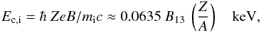 (1)where A is the mass number of the ion ( ≈ 1 for H and ≈ 56 for Fe), Z is the ion charge, mi is the ion mass, B13 = B / 1013 G, and some boundary energy EC, which can be estimated as
 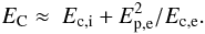 (2)Here Ep,e is the electron plasma energy
 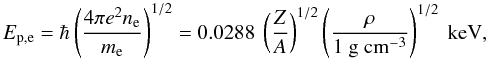 (3)and Ec,e is the electron cyclotron energy
  (4)where ne is the electron number density, ρ is the mass density, and me is the electron mass.
Only one radiation mode can propagate between Ec,i and EC, therefore the radiation emissivity is approximately a factor of two lower in this range. The condensed surface density depends on magnetic field and chemical composition (e.g., Lai 2001)  (5)where η′ is a coefficient ranging probably between 0.5 and 1 (see discussion in van Adelsberg et al. 2005). Therefore, the plasma energy at the surface can be expressed as (van Adelsberg et al. 2005)
 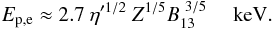 (6)We conclude that it is possible to estimate the equivalent width of this absorption feature as
 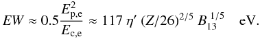 (7)In all calculations below, we used η′ = 1.
The second feature is at the plasma energy Epe, which is far less important for us. The observed absorption lines lie at E < 1 keV, which would correspond to the plasma energy at B < 6.4 × 10¹¹ (Z / 26) − 1 / 3 G. Meanwhile, the critical temperature for the plasma phase transition leading to the formation of the condensed surface is roughly  K (Potekhin et al. 1999; Lai 2001). We note that the observed temperatures of the XDINSs are about 106 K, and conclude that the absorption feature at the plasma energy in the condensed surface radiation cannot be of energy any lower than 1 keV in these stars. Therefore, the observed absorption features in XDINSs cannot be associated with the absorption feature at the plasma energy. However, the first absorption feature (between Ec,i and EC) may be prominent in their spectra.
The angular distribution of the condensed surface emissivity can be estimated from the results of van Adelsberg et al. (2005)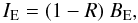 (8)where BE is Planck function,
 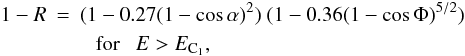 (9)
(9) (10)
(10) (11)and
 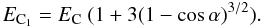 (12)Here α is the angle between radiation propagation direction and the surface normal, and Φ is the angle between the surface normal and the magnetic field lines. This approximation is presented graphically in Fig. 1 with accurate calculations, performed using the method described by van Adelsberg et al. (2005) in the free ions approximation.
Here we neglect the angular dependence on the azimuthal angle ϕ between radiation propagation plane and the normal-magnetic field line plane for the inclined magnetic field (see Fig. 6 in van Adelsberg et al. 2005) and the absorption feature at Epe. We also ignore damping effects, which smooth the transitions between different bands. This approximation leads to sharp boundaries at Ec,i and EC1 in the computed spectra (Figs. 3, 4, 6–8, 13), which can be smoother in more detailed computations (see, however, next paragraph). In our approximation, we ignore the azimuthal dependence of R in the case of an inclined magnetic field. At some azimuthal angles, the absorption feature considered can be less significant (see Fig. 4 in van Adelsberg et al. 2005). Therefore, our calculations with this approximation provide an upper limit to the strength of the absorption feature. This effect must be less significant in the case of a thin model atmosphere above the condensed surface due to significant atmospheric optical depth in the X-mode around the proton cyclotron resonance (see Fig. 5).
Our approximation appears rough, but the more accurate calculations of R also have significant uncertainties. First of all, these calculations were performed after making two different approximations: a complete neglect of ion motions, and free ions. The real picture is in some sense intermediate. Ions in the crystal grid (or in liquid) are not free, but can move. These two limits provide very different spectra at energies below Ec,i (see Figs. 2–6 in van Adelsberg et al. 2005). The approximately known factor η′, which determines the value of EC and the width of the absorption feature, was already mentioned above. Moreover, the accurate calculations are applicable only to a perfectly smooth condensed surface. If the surface has some roughness, the emitted spectrum must be close to resembling a black body (van Adelsberg et al. 2005). Our approximation corresponds to the free-ions limit and produces radiation spectra reflecting the main features of condensed surface spectra, especially if we take into account all the uncertainties mentioned above.
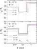 |
Fig. 1 Approximation of dimensionless emissivity as a function of photon energy E for the case of a condensed iron surface at B = 1013 G. Top panel: the magnetic field is normal to surface. The different curves correspond to different angles α between emergent photon direction and surface normal. Bottom panel: the emergent photon direction is inclined 45° to the surface. The different curves correspond to different angles Φ between magnetic field lines and surface normal. |
2.2. Model atmospheres of magnetized neutron stars
Many scientific groups have computed model atmospheres of magnetized neutron stars, but we use our own calculations to describe of the radiation spectra. We employ the code presented by Suleimanov et al. (2009), where details of the computational method can be found.
Here we assume that the magnetic field strengths of the XDINSs are about a few 1013 G and consider a pure hydrogen atmosphere. The effective temperatures are ≈ 106 K. At these values of B and T, hydrogen is partially ionized (Potekhin et al. 1999) and the vacuum polarization effect and the partial mode conversion can be significant (Ho & Lai 2003; van Adelsberg & Lai 2006). The model atmospheres presented below therefore include these effects. The magnetic field in presented models is assumed to be homogeneous and normal to the surface. In general, it is necessary to study model atmospheres with inclined magnetic field when modeling the integral spectra of neutron stars (Ho et al. 2008). However, we consider the general features of the model spectra, and therefore neglect the distinctions between spectra of the models with different field inclinations, which are unimportant to the qualitative behavior of the spectrum (see corresponding figures in Shibanov et al. 1992; Suleimanov et al. 2009). In addition, the bright regions at magnetic poles of a star in our models considered below have magnetic fields close to normal.
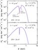 |
Fig. 2 Emergent spectra of two thin model atmospheres above a black-body condensed surface (solid curves) with Teff = 1.2 × 10⁶ K and B = 4 × 10¹³ G together with fitting spectra (dashed curves). The fitting spectra are black-body spectra with the color temperature Tc = fcTeff and two Gaussian lines. Top panel: the spectrum of the model with surface density Σ = 10 g cm-2. Parameters of the fitting spectrum: fc = 1.2, D = 1.14-4, center of the first line (proton cyclotron) E1 = 0.25 keV, optical depth τ1 = 2.6, and width σ1 = 6 eV, and for the second line (H bound-bound transitions) E2 = 0.3 keV, τ2 = 1.1, σ2 = 40 eV. Bottom panel: the spectrum of the model with surface density Σ = 1 g cm-2. Parameters of the fitting spectrum: fc = 1.12, D = 1.12-4, line parameters are the same as above, except τ2 = 0.08. |
The emergent spectra of two thin magnetized model atmospheres (i.e., a hydrogen layer above a condensed surface) with parameters typical for the XDINSs are shown in Fig. 2. We display the Eddington flux  (13)where IE is a specific intensity. Later we also use the astrophysical flux FE = 4HE. The physical flux often used is defined to be ℱE = πFE = 4πHE. For black-body radiation, it is FE = IE = BE. In the models shown in Fig. 2, the black-body radiation is used as the inner boundary condition for the radiation transfer equation. There are absorption features in the spectra, which are produced by the proton cyclotron absorption and bound-bound and bound-free transitions in hydrogen atoms. We note that the proton cyclotron feature is weakened by vacuum polarization and partial mode conversion, but remains prominent in the spectra, as can be seen in our figures below (see also Suleimanov et al. 2009). Equivalent widths (EWs) of these features are ≈ 25 eV and ≈ 90 eV for the models with surface densities Σ = 1 and 10 g cm-2, respectively. The absorption feature in the spectrum of a semi-infinite atmosphere is less prominent than in the model with Σ = 10 g cm-2 (see Suleimanov et al. 2009) and has a smaller EW ( ≈ 50 eV). The EW of the model absorption feature depends slightly on the magnetic field strength and the relation between proton cyclotron energy and kTeff. For example, the EW of the absorption feature is close to 80 eV in the model with B = 1014 G, Σ = 10 g cm-2, and the same Teff (see Fig. 4).
The spectra of these models can be fitted approximately by diluted black-body spectra BE with a color temperature Tc slightly higher than the effective temperature Teff and two Gaussian absorption lines given by  (14)where fc = Tc / Teff is the hardness factor and D is the dilution factor, which can differ from the usual
  . We later present the dilution factor in the form
  to distinguish it from the usual value. The optical depths of the absorption lines at a given photon energy E are
 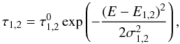 (15)where
  are the optical depths at the centers of the lines at energy E1,2 and σ1,2 are the line widths. The values of these fitting parameters for these two spectra are given in the caption of Fig. 2. The first line corresponds to the proton cyclotron line in the model atmosphere spectra, and the second corresponds to the bound-bound transitions in hydrogen atoms (cf. Potekhin & Chabrier 2004; Potekhin et al. 2004).
It is clear that the black-body radiation model is not an accurate inner boundary condition for the thin model atmospheres above the condensed surfaces, and that the true radiation properties of the surface have to be used when performing precise modeling. Below we use our approximations in Eqs. (9)–(11) for the inner boundary conditions of radiation transfer equation for both radiation modes, extraordinary (X) and ordinary (O) 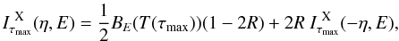 (16)
(16) (17)where η = cosα, and I X,O are the specific intensities of the extraordinary and ordinary modes. In future work, we plan to replace this approximation by accurately computed radiation properties of the condensed surfaces. But we expect the present approximation to be qualitatively correct.
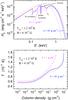 |
Fig. 3 Emergent spectra (top panel) and temperature structures (bottom panel) of thin partially ionized hydrogen atmospheres (Teff = 1.2 × 10⁶ K, B = 4 × 10¹³ G) above a condensed iron surface with Σ = 10 g cm-2 (solid curves) and Σ = 1 g cm-2 (dashed curves). An inner boundary condition for the radiation transfer equation, corresponding to the condensed surface radiation properties (see text), was used. The black-body spectra with T = Teff (dotted curve) and the diluted black-body spectra (fc = 1.5, D = 1.3-4), which describe the high-energy part of the spectrum of the atmosphere with Σ = 1 g cm-2 (dash-dotted curve) are shown for comparison in the top panel. In the bottom panel, the temperature structure of the model with Σ = 10 g cm-2 using black-body radiation as the inner boundary condition is also shown (dotted curve). |
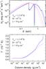 |
Fig. 4 Effect of the inner boundary condition of the radiation transfer equation on emergent spectrum (top panel) and temperature structure (bottom panel) of a thin partially ionized hydrogen atmosphere (Teff = 1.2 × 10⁶ K, B = 1014 G) with Σ = 10 g cm-2, above the condensed iron surface (solid curves) and black-body surface (dashed curves). For comparison, the black-body spectrum with T = Teff (dotted curve) and the diluted black-body spectrum (fc = 1.6, D = 1.4-4), with a Gaussian line representing the proton cyclotron line (E1 = 0.63 keV, τ1 = 8.5, σ1 = 11 eV), and a half-Gaussian line (E2 = 0.3 keV, τ1 = 2.5, σ1 = 150 eV) describing the absorption feature at energies higher than Ec,i (dash-dotted curve) are shown. That last curve fits the spectrum of the atmosphere above the condensed iron surface. |
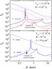 |
Fig. 5 Optical thickness of a thin partially ionized hydrogen atmospheres with Teff = 1.2 × 10⁶ K above the condensed iron surface in X-mode (solid curves) and O-mode (dashed curves). Top panel: B = 4 × 10¹³ G and Σ = 1 and 10 g cm-2. Bottom panel: B = 1014 G and Σ = 10 g cm-2. |
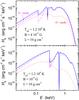 |
Fig. 6 Total emergent spectra (solid curves) together with spectra in the X-mode (dashed curves) and in the O-mode (dotted curves) of a thin partially ionized hydrogen atmosphere with Teff = 1.2 × 10⁶ K, Σ = 10 g cm-2 above the condensed iron surface with B = 4 × 10¹³ G (top panel), and B = 1014 G (bottom panel). |
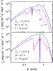 |
Fig. 7 Emergent specific intensity spectra of two model atmospheres above a condensed iron surface with Teff = 1.2 × 10⁶ K, Σ = 10 g cm-2, and B = 4 × 10¹³ G (top panel) and B = 1014 G (bottom panel). Spectra at different angles between radiation propagation and surface normal are shown: 1° (solid curves), 30° (dashed curves), 60° (dotted curves), and 75° (dash-dotted curves). |
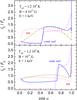 |
Fig. 8 Angular distributions of the emergent radiation at photon energy 1 keV. Top panel: models with Teff = 1.2 × 10⁶, B = 4 × 10¹³ G above the condensed iron surface and Σ = 10 g cm-2 (solid curve), Σ = 1 g cm-2 (dashed curve), Σ = 10 g cm-2 above a black-body (dotted curve), and a semi-infinite atmosphere (dash-dotted curve). Bottom panel: models with Teff = 1.2 × 10⁶, B = 1014 G and above the condensed iron surface with Σ = 10 g cm-2 (solid curve), Σ = 1 g cm-2 (dashed curve), Σ = 10 g cm-2 above a black-body (dotted curve), and a semi-infinite atmosphere (dash-dotted curve). |
We computed thin hydrogen model atmospheres above condensed iron surfaces using these new inner boundary conditions. The results are presented in Figs. 3–8. Model atmospheres are optically thick in the O-mode in the observed part of the X-ray band (0.1–5 keV), and almost everywhere optically thin in the X-mode. Therefore, the total spectra are defined mostly by the X-mode spectra, because the O-mode spectrum originates in the cooler layers of the atmosphere.
The emergent spectra of the thin magnetized model atmospheres above the condensed surface are harder (fc ~ 1.5 − 1.7) than models above a black body, because the temperatures at the inner boundaries of these models are higher (see bottom panels in Figs. 3–4).
Because of the condensed surface emission properties, broad absorption features appear between Ec,i(Fe) and approximately EC, which are especially prominent at Ec,i. The dependence of optical depths of thin atmospheres in both modes on the photon energy are shown in Fig. 5. The atmospheres are optically thin in the X-mode at almost all energies, except the region around the proton cyclotron energy. The total spectra are dominated by the X-mode (see Fig. 6), hence are close to the condensed iron spectra in the X-mode, especially in the Wien tail. However, this is not the case for the band between Ec,i(Fe) and EC. In this region, the O-mode flux can contribute a significant part to the total flux (see Fig. 6). At energies in the vicinity of Ec,i(H), the opacity in the X-mode increases, hence the optical depth of atmosphere and the emergent flux also increase. As a result, a complex absorption feature is produced with a total EW ≈ 400 eV for the model with B = 1014 G and Σ = 10 g cm-2, EW ≈ 370 eV for B = 4 × 10¹³ G and Σ = 1 g cm-2, and EW ≈ 260 eV for B = 4 × 10¹³ G and Σ = 10 g cm-2. We note that the EWs of these features are larger than the sums of the EWs of the cyclotron line in the atmosphere spectra and the EWs of the absorption feature in the condensed surface spectra (see Eq. (7)). The reason for this difference is the following. Between Ec,i and EC, a naked condensed surface radiates mainly in the O-mode, which has approximately half of the flux of modes at other energies. In contrast, a thin atmosphere above the condensed surface is optically thick in the O-mode, and the emergent flux forms in the upper atmosphere layers, which have significantly lower temperatures than the condensed surface. Therefore, the emergent flux in this band is significantly lower than the naked condensed surface. This is particularly true for the model with B = 1014 G.
In addition to the spectral energy distribution of the emergent flux, the angular distribution is also important. Examples of angular distributions for various models of magnetized atmospheres are shown in Figs. 7–8. There is a narrow spike at the surface normal, but the total energy radiated in this spike is relatively small and we neglect these spikes below. Angular distributions of semi-infinite magnetized atmospheres have maxima at α ≈ 40°–60° (Pavlov et al. 1994). An example of such a distribution is presented in the bottom panel of Fig. 8. It can be fitted by the function 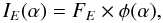 (18)where
  (19)The angular distributions of the specific intensities of the thin magnetized atmospheres above a black body are close to isotropic (Fig. 8). The corresponding distributions for the atmospheres above condensed surfaces are also almost isotropic (see Fig. 8), but have some interesting features at energies between EC and 4EC. The location of the high energy boundary of the broad depression depends on α (see Eq. (12)). Therefore, at a given photon energy there is an angle α corresponding to this location. At this angle, the specific intensity angular distribution has a jump. At relatively small angles, the distribution corresponds to the usual angular distribution for the model atmosphere, but at larger angles, the specific intensities are significantly smaller (see Fig. 8). This jump is more prominent for the model with B = 4 × 10¹³ G and is also clearly visible in the spectra for the specific intensities of this model (the top panel of Fig. 7). In the angular distributions of the intensities of the model with B = 1014 G, this jump is less significant (Figs. 7 and 8), because for this model EC ≈ Ec,i(H) and the X-mode opacity is more important, in addition to the mode conversion. The features of the magnetized model atmospheres are very unusual and have to be studied in more detail with a more accurate treatment of the radiation properties of the condensed surfaces.
From the presented examples of the partially ionized hydrogen magnetized model atmospheres, we can conclude that they display complex absorption features with EW ≲ 100 eV in the spectra. The naked condensed surfaces can have broad absorption features with slightly larger EWs ( ≥ 120 eV), but the absorption structures in the spectra of thin atmospheres above condensed surfaces can have significantly larger EWs, up to 400 eV.
3. Calculation method for the integral neutron star spectrum
We consider a slowly rotating spherical isolated neutron star with given compactness M / R as a model for XDINS spectra and light-curve fitting, taking into account distributions of the local temperatures and magnetic field strengths over the stellar surface. Local spectra are black-body-like spectra with corresponding temperature and absorption lines, whose central energies depend on the local magnetic field. Gravitational redshift and the light bending are taken into account.
The geometry of our model is shown in Fig. 9. The magnetic axis is inclined to the rotation axis by the angle θB, and i is the inclination angle of the rotation axis relative to the line of sight. The phase angle ϕ is the angle between the plane containing the rotation axis and the line of sight and the plane containing the magnetic and rotation axes. One magnetic pole can be shifted relative to the antipode of the other pole by a small angle κ. We assume that the brightest areas of the NS surface are located at the magnetic poles. Therefore, the temperature and magnetic field distributions close to the poles are the most important.
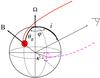 |
Fig. 9 Geometry of the model. The opposite bright spot is indicated by the dashed circle. |
XDINSs pulse fractions are significant, and a classical temperature distribution, produced by the global (core) dipole magnetic field of a NS, is insufficient to reproduce observed pulse fractions (Page 1995; Geppert et al. 2006). Schwope et al. (2005) showed that the RBS 1223 light curves can be fitted by two models, namely two bright isothermal spots with different temperatures, or two narrow peaked temperature distributions (with different parameters) taken from Geppert et al. (2004). Geppert et al. (2004) considered the thermal transport in the NS crust for a poloidal dipole magnetic field, concentrated in the crust only. In this case, the magnetic field lines have large inclinations to the surface normal in a wider band around the magnetic equator than in the global dipole field case. The thermal conductivity across magnetic field lines is lower than along them, therefore the bright spots around magnetic poles are brighter and smaller than they would be for the dipole distribution. Another possibility is a strong toroidal magnetic field in the NS crust. Using various approximations, these models were computed by Pérez-Azorín et al. (2006a), who derived an analytical approximation of the surface temperature distribution for the crust magnetic field with a strong toroidal component calculated for the force-free conditions. We use this approximation for the temperature distribution in our model.
In a well-known approximation by Greenstein & Hartke (1983), the temperature distribution is 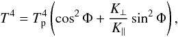 (20)where K ⊥ and K ∥ are thermal conductivities across and along the magnetic field, respectively, and Tp is the temperature at the magnetic pole. Magnetic fields of the isolated NSs can be strong enough (~1013 G) for the ratio K ⊥ / K ∥ to be small. In this case, the temperature distribution can be approximated as (Pérez-Azorín et al. 2006b)
 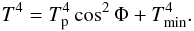 (21)In the force-free approximation, a simple relation between the magnetic colatitude θ and the magnetic field inclination in the NS crust was suggested by Pérez-Azorín et al. (2006a)
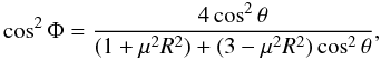 (22)where μ-1 is a typical toroidal magnetic field length scale, and μR is an approximate ratio of the toroidal component of the magnetic field to the poloidal one. The case μ = 0 corresponds to a core dipole magnetic field. Although this magnetic field model was derived for the crust, we also use Eq. (22) in the atmosphere, because it allows us to investigate the possible effects of magnetic field and temperature inhomogeneity by changing a single parameter μ. Finally, we use the following temperature distributions around magnetic poles
 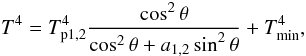 (23)where
 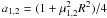 and Tp1,2 are the temperature distribution parameters. This can describe various temperature distributions (see Fig. 10), from strongly peaked (a ≫ 1) to a classical dipolar (a = 1 / 4) or homogeneous (a = 0) distribution.
Another possibility is to consider two isothermal bright spots around the magnetic poles with fixed temperatures and angular sizes.
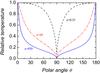 |
Fig. 10 Temperature distributions at various parameters a. Only the first term on the right-hand side of Eq. (23) is used for these calculations. |
The surface magnetic field distribution, which corresponds to the magnetic field inclination in the force-free approximation model (Eq. (22)) is described by 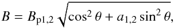 (24)where Bp1,2 are the magnetic field strengths at the poles.
Temperature and magnetic field distributions are calculated separately around each magnetic pole, therefore, the distributions are not smooth at the magnetic equator area if one of the poles is shifted. But this small mismatch at the equator is unimportant, because this area is dim.
The local spectrum of the NS surface in the case of magnetized atmospheres at given temperature and magnetic field is taken as a diluted black-body spectrum with two additional absorption features (see also Eqs. (14), (15) and (18))  (25)where the optical depth τi of the absorption line i at given photon energy E is defined by Eq. (15), and
  , σ1,2 are considered as model parameters identical for all NS surface elements. The photon energy of the line center Ei depends on the local magnetic field strength B. In particular, for the proton cyclotron line we have
  (26)For the description of the local spectra of the model atmospheres above a condensed iron surface, two additional absorption features can be considered. The first feature is centered on the iron ion cyclotron energy according to Eq. (1). This line is asymmetric, i.e., τ2 > 0 only for E > E2, in agreement with the calculations (see Figs. 3 and 4). The second line is centered between E1 and EC, and its position depends also on the local magnetic field strength.
We use three angular distributions φ(α) of the specific intensity IE(α). The simplest is the isotropic function φ(α) = 1, which corresponds to the thin model atmosphere above a black body. For the semi-infinite model atmosphere, the angular distribution in Eq. (19) are used. For the thin atmosphere models above a condensed iron surface, the isotropic angular distribution is used except for the energy band between EC and 4EC, where the angular distribution has a jump at some cosα (see Fig. 8), a case that has to be studied separately.
For the description of the naked condensed surface spectra, the relations in Eqs. (8)–(12) are used.
The total spectrum of the NS is calculated in the spherical coordinate system connected with the rotation axis (see, for example, Poutanen & Gierliński 2003 and references therein)  (27)where d is the NS distance and γ is the angle between the radius vector at a given point and the rotation axis. Here the observed and the emitted photon energies are connected by the relation E = E′(1 + z)-1, and z = (1 − RS / R) − 1 / 2 − 1 is the gravitational redshift. Light bending in the gravitational field is accounted for by the approximate relation (Beloborodov 2002)
  (28)where RS = 2GM / c2 is the Schwarzschild radius, and
  (29)The integration in Eq. (27) is restricted to the visible NS surface area with cosα > 0.
Phase-resolved spectra can be calculated for various phase angles, and the corresponding light curves can also be calculated for various energy bands. The mean spectrum is summed from separate phase spectra and then divided by the number of phases.
Using this code, we calculated two test light curves for slowly rotating neutron stars (see Fig. 11). The first one corresponds to the light curve presented by Poutanen & Gierliński (2003) in their Fig. 4a (dashed curve), and the second one corresponds to Class III light curves in the classification performed by Beloborodov (2002) (see his Fig. 4).
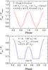 |
Fig. 11 Test light curves calculated with the same parameters as used by Poutanen & Gierliński (2003) (top panel) and Beloborodov (2002) (bottom panel). F1 is the maximum possible flux that is observed when one of the spots is viewed face-on. |
4. Results of modeling
We present examples of model light curves and integral emergent spectra for magnetized neutron stars with various surface temperature distributions. We choose symmetric models with equal temperatures and magnetic field strengths at both magnetic poles, and equivalent temperature and magnetic field distributions in both hemispheres. We consider a neutron star model with polar temperature kTp = 0.15 keV, polar magnetic field strength Bp = 6 × 10¹³ G, and a compactness corresponding to the gravitational redshift z = 0.2. Three temperature distributions are used. Two of them are described by Eq. (23) with a = 0.25 and a = 60. In both distributions, Tmin equals 0.316Tp. The results are almost the same for any lower value of Tmin. The third temperature distribution is a uniform surface temperature kT = 0.01 keV plus two uniform bright spots around the magnetic poles with the same temperatures Tp and angular radii θsp = 5°. Most of the models are calculated for angles i = θB = 90°, which provides the largest change in the visible local parameters during a rotation period. For simplicity, we take dilution D and the hardness fc factors equal to 1. Most of our results will not be changed by this; in particular, the normalized spectra and EWs of absorption lines will not change, if fc and D are constant over the neutron star surface. This approximation will only change the absolute value of the flux. Therefore, it is important for the ratio of X-ray to optical fluxes, because fc and D can be different for X-ray and optical bands (see Sect. 4.3). Therefore, in this section we consider the temperature distribution over the neutron star to be a color temperature distribution instead of an effective temperature distribution.
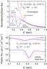 |
Fig. 12 Phase-averaged photon spectra for the neutron star model with kTp1 = kTp2 = 0.15 keV, Bp1 = Bp2 = 6 × 10¹³ G, z = 0.2, i = θB = 90° and different temperature distributions across the surface. Top panel: the temperature distribution Eq. (23) with a1 = a2 = 0.25 (dotted curve), with a1 = a2 = 60 (dashed curve), and two uniform bright spots with T = Tp and angular size θsp = 5° (solid curve). The local spectra are isotropic black-body spectra with an absorption line (τ1 = 3, σ1 = 30 eV) centered according to Eq. (26). The spectrum of the model with a = 0.25 and a weaker absorption line (τ1 = 2.6, σ1 = 6 eV) is also shown (dash-dotted curve). The thin solid curves are the continuum spectrum of a model with a = 60 and a single black-body spectrum with a Gaussian line (E1 = 0.25 keV, τ1 = 0.85, σ1 = 52 eV) for the strong-line a = 0.25 model. Bottom panel: the photon spectra for two temperature distributions (a = 0.25 and two bright spots) under various inclination angles to the line of sight: i = 0° (solid curves), i = 45° (dashed curves), and i = 90° (dotted curves). |
4.1. Averaged spectra
The main goal of our modeling is to study possible absorption features in the magnetized neutron star thermal spectra. To achieve this aim, the spectra of the models with the three temperature distributions, as described above, and the three local spectral energy distributions, as described in Sect. 2, are computed. In all cases, we consider the color temperature distribution over the neutron star surface.
4.1.1. Black body plus Gaussian line
The first spectral model is a simple isotropic black-body spectrum with a temperature equal to the local temperature of a given model and one Gaussian spectral line. The line is centered on the proton cyclotron energy (see Eq. (26)) and has parameters τ1 = 3, σ1 = 30 eV, hence EW ≈ 100 eV. This model roughly represents the shape of the spectrum of a thin magnetized partially ionized hydrogen atmosphere above the black-body condensed surface (see Fig. 2). The same model can represent the shape of the spectrum of the semi-infinite atmosphere at the maximum of the flux, but, of course, with higher fc. Model spectra of semi-infinite magnetic atmospheres have harder tails than a black body. To first approximation, these spectra at maximum flux can however be described as diluted black-body spectra (see, for example, Suleimanov & Werner 2007 for non-magnetic atmospheres). Moreover, the model spectra with vacuum polarization and partial mode conversion have smaller deviations from a blackbody than the models, where these effects are ignored (see Fig. 10 in Suleimanov et al. 2009). We mainly investigate the absorption features, and ignore the harder spectral tail in the model atmosphere spectra.
Integral photon spectra for all the temperature distributions are shown in the top panel of Fig. 12. The overall shapes of the spectra can be described by black-body spectra with kT ≈ 0.114 keV for the model with a = 0.25, kT ≈ 0.086 keV for the model with a = 60, and kT ≈ 0.125 keV for the model with two bright spots. Therefore, these spectra can be described to first approximation by single black-body spectra with a Gaussian line. An example of this approximation is shown in Fig. 12. The model spectrum with a = 0.25 is represented well by the black-body spectrum with kT ≈ 0.114 keV and a Gaussian line with E1 = 0.25 keV, τ1 = 0.85, σ1 = 52 eV. The integral spectra have a soft excess and an asymmetric line compared to single blackbody spectra. These features increase if a increases (see also Fig. 17).
The spectrum of the model with a = 60 is the softest caused by the relatively large contribution of the cooler parts of the neutron star. The spectrum of the two spot model has a relatively narrow absorption line, because most radiation comes from the pole regions where the magnetic field strength is nearly constant. The spectrum of the model with a = 0.25 shows a wide asymmetric line, shifted to lower energy. The large width of the line is a consequence of the smooth temperature distribution, and, accordingly, a large variety of magnetic field strengths, which effectively contribute to the spectrum. The absorption feature in the spectrum of the model with a = 60 is very wide and difficult to see. It can be recognized by comparison with the spectrum without the line (the thin curve in Fig. 12, top panel). In the model, the magnetic field changes significantly, from Bp at the poles to 7.7Bp at the equator, and the absorption line is strongly smoothed. An observable absorption feature appears only in models with a ≤ 10 − 50 (depending on the EW of the local absorption line). Therefore, strong toroidal fields on the surface of XDINSs (corresponding to a > 50) are incompatible with the observed absorption lines.
The equivalent widths of these absorption features range from 65 eV (a = 60 model) to 85 eV (the other models). Therefore, the magnetic field distribution does not result in an increase of the EW of the absorption line in the integral spectrum. For illustration, the integral spectrum of the model with a = 0.25 and a line with τ1 = 2.6, σ1 = 6 eV, and EW ≈ 19 eV is also shown in the upper panel of Fig. 12. The line has a significant width but a small depth with EW ≈ 17 eV.
The integral spectra of the model with a = 0.25 and the two-spot model at different inclination angles of the magnetic axis and rotation axis (which coincide), to the line of sight (i = 0°, 45° and 90°) are shown in the bottom panel of Fig. 12. These spectra represent phase-resolved spectra at various phases of the stellar rotation for the case θB = 90°. The spectra of the two-spots model only exhibit the flux level variation, without any change in line shape. In contrast, the spectra of the models with a = 0.25 exhibit line shape variations. At larger i, the line center is shifted to lower energy and becomes wider, because a more significant part of the observed radiation comes from the magnetic equator regions. The dependence of the absorption line EW on the inclination angle is insignificant.
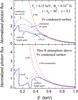 |
Fig. 13 Top panel: phase-averaged photon spectra of the same neutron star models as in Fig. 12, but here the local spectra are from a naked iron surface. The continuum spectra without absorption features are shown by the thin solid curves for the two-spots model and the model with a = 0.25. Bottom panel: phase averaged photon spectra of the same neutron star models as in Fig. 12, but here the local spectra are isotropic blackbodies with absorption features as in the spectra of the thin hydrogen model atmosphere above the condensed iron surface (see text). The continuum spectrum without absorption feature is shown by the thin solid curve for the model with a = 60. |
4.1.2. Naked condensed iron surface
The second model used for the local spectrum is the spectrum of the naked condensed iron surface, provided by Eqs. (8)–(12). The computed spectra for the neutron star models with the same parameters and temperature distributions, as in the case of the first local model, are shown in the top panel of Fig. 13. These integral spectra are close to being black-body spectra with similar color temperatures, as in the first case (see Sect. 4.1.1). The absorption features are very wide and shallow and have EWs equal to ≈ 110 eV for the two-spots model, ≈ 140 eV for the model with a = 0.25, and ≈ 95 eV for the model with a = 60. In the last case, the line is again not observable, and the EW is obtained with a lower accuracy because of uncertainties in the continuum definition.
It is possible to compare approximate calculations of neutron star spectra that have a naked condensed iron surface with the accurate calculations performed by the method described in van Adelsberg et al. (2005). An example of this comparison is shown in Fig. 14. The qualitative agreement is satisfactory. The accurate spectrum is (as expected) more smooth at EC, and the flux at energies less than Ec,i is higher. The EWs of the absorption features are very similar, ≈ 190 eV for the accurate spectrum and ≈ 180 eV for the approximate spectrum.
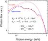 |
Fig. 14 Phase averaged photon spectra of the neutron star models with parameters kTp1 = kTp2 = 0.15 keV, Bp1 = Bp2 = 6 × 10¹³ G, i = θB = 0° and a = 0.25. The local spectra are from a naked iron surface, computed accurately using the code presented by van Adelsberg et al. (2005) (thick solid curve), and using approximate Eqs. (8)–(12) (thick dashed curve). The adopted continuum spectra without absorption features are shown by the corresponding thin curves. The EWs of the absorption features are rather similar, ≈ 190 and 180 eV. |
4.1.3. Thin atmosphere above condensed iron surface
The shape of the spectrum of a thin hydrogen atmosphere above a condensed iron surface can be roughly fitted by a black-body spectrum with two absorption features in Gaussian profiles, which describe the proton cyclotron line and one half of the wide line at Ec,i(Fe). The half line means that the line optical depth is equal to zero at energies E < Ec,i(Fe), and calculated in the usual way (Eq. (15)) at E > Ec,i(Fe). For our illustrative calculations, we assume that τ1 = 8.5, σ1 = 11 eV, and τ2 = 2.5, σ2 = 150 eV with a total EW ≈ 230 eV (see also Fig. 4). The Gaussian lines with these τi and σi reproduce well the absorption features in the spectrum of the thin hydrogen atmosphere above the condensed iron surface with Teff = 1.2 × 10⁶ K, B = 1014 G, and Σ = 10 g cm-2 (Fig. 4). The computed spectra for the used temperature distributions are shown in the bottom panel of Fig. 13. The temperature of the neutron star surface again corresponds to the color temperature. The hard tails of the integral spectra can be fitted by the black-body spectra with approximately the same temperatures as those obtained for the first local spectral model. The absorption feature has a prominent two-component structure for the two-spots model, and a smoothed shape for the model with a = 0.25. In the spectrum of the model with a = 60, the absorption line is again very smooth. The EWs of the features in spectra of the two-spot model and the model with a = 0.25 are ≈ 210 eV, and the EW of absorption feature in the spectrum of the model with a = 60 is ≈ 150 eV.
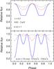 |
Fig. 15 Examples of light curves for the neutron star model with kTp1 = kTp2 = 0.15 keV, Bp1 = Bp2 = 6 × 10¹³ G, z = 0.2, i = θB = 90° and different temperature distributions across the surface: the temperature distribution (23) with a1 = a2 = 0.25 (dotted curves), with a1 = a2 = 60 (dashed curves), and two uniform bright spots with T = Tp and angular size θsp = 5° (solid curves). Two different angular distributions of the emergent radiation are used: the isotropic distribution (top panel) and the semi-infinite magnetic atmosphere distribution Eq. (19) (bottom panel). |
4.2. Light curves
Light curves calculated for illustrative purposes in a wide energy band (0.02–2 keV) are shown in Fig. 15. The light curves are computed for the orthogonal rotator (i = θB = 90°), the three temperature distributions, and two angular distributions of the emergent flux, i.e., the isotropic one and the distribution corresponding to a semi-infinite magnetized hydrogen model atmosphere as described by Eq. (19). The light curves, computed with the isotropic angular distribution, agree with the well-known result (see, e.g. Page 1995; Geppert et al. 2006) that the temperature distribution for a core dipole magnetic field (a = 0.25) cannot provide a pulsed fraction PF ≡ (Fmax − Fmin) / (Fmax + Fmin) larger than several percent. To account for larger PF values, more peaked temperature distributions have to be considered (Schwope et al. 2005). Computed light curves have PF ≈ 5% for the temperature distribution with a = 0.25, ≈10% for a = 60, and ≈ 25% for the two bright spots.
Using the angular distribution corresponding to the magnetized model atmosphere, we obtain completely different pulse profiles with four maxima instead of two for the isotropic angular distributions (bottom panel in Fig. 15). The model with a = 0.25 shows additional maxima at the phases of the minima in the light curve computed with isotropic angular distribution. The models with the narrow peaked temperature distributions (two spots and a = 60) exhibit deep minima at the phases of the maxima in the light curves computed by assuming an isotropic angular distribution. Each minimum in these light curves is replaced by two maxima with a shallow minimum between them. The pulsed fractions of the light curves for the models with a = 0.25 and a = 60 are the same as in the isotropic distribution case, but the pulsed fraction of the light curve for the model with two bright spots increases to 60%. A qualitatively similar class III light curve for a slowly rotating neutron star with magnetic atmosphere model radiation was obtained by Ho (2007) (see his Fig. 2).
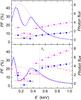 |
Fig. 16 Energy dependence of pulsed fractions (symbols and left vertical axes) together with averaged photon spectra (lines and right vertical axes) for the neutron star models with the same parameters as in Fig. 12 and a = 0.25. Top panel: the models with pure black-body local spectra (open circles and dotted curve), black-body local spectra with an absorption line (τ = 3.0, σ = 30 eV) centered according to Eq. (26), and the isotropic angular distribution (filled circles and solid curve), and black-body local spectra with the absorption line and the electron scattering atmosphere angular distribution (triangles and dashed curve). Bottom panel: the model of a naked condensed iron surface (open circles and dotted curve), a thin atmosphere above condensed iron surface spectra with corresponding angular distribution (filled circles and solid curve), and the same local spectra, but with slightly different pole temperatures: Tp,1 = 0.15 keV, Tp,2 = 0.14 keV (triangles and dashed curve). The position of EC, which corresponds to the magnetic pole, is shown by vertical dotted line. |
We also investigate the influence of the absorption features on light curves and pulsed fractions. In a wide energy band, the influence on the light curves is very small. However, it is significant on both the light curves and pulsed fractions in the narrow energy bands in the vicinity of the absorption feature energies. For illustration, we calculate the dependences of PF on the photon energy for the models with a smooth temperature distribution (a = 0.25) and the different local spectra (see Fig. 16). The corresponding average spectra are presented in the same figure for illustrative purposes. The common characteristic of all the presented dependences is the decrease in the pulsed fraction at the absorption feature energies.
In the top panel of Fig. 16, the local spectrum is approximated by the black body with and without an absorption line, and the change in the pulsed fraction at the absorption line energies can be clearly seen. The PF for the bolometric light curve ( ~ 5%) is determined by the soft part of the spectrum, where most of the photons originate. The PF can be more significant for the higher energy bands. We also calculate the average spectrum and the PF dependence on energy using the same model but a more peaked angular distribution of the local emergent radiation for an electron scattering atmosphere  (30)The average spectrum is altered insignificantly, but the pulsed fraction is increased by a factor of two (the top panel in Fig. 16). We present this result to demonstrate that a pencil-like peaked angular distribution of the emergent radiation can have an effect, similar to the effect of a peaked temperature distribution.
The dependence of the pulsed fraction on energy for the models with local spectra corresponding to a naked iron surface and a thin atmosphere above the condensed iron surface is similar (the bottom panel in Fig. 16). The PF at energies E > EC is larger because of the peaked angular distributions (see Eqs. (8)–(12) and Fig. 8). In our calculations, we approximate the angular distribution of the thin atmosphere above the condensed surface emergent radiation using a simple step function in the EC–4EC energy range 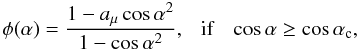 (31)and
  (32)where
 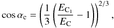 (33)and aμ is a parameter, which is taken to be 0.2 here. At other energies, φ(α) = 1 is used.
The pulsed fraction at these energies can be even more significant if slightly different temperatures at the poles are used. Here we do not take into account the azimuthal dependence of the angular distribution of the magnetized semi-infinite atmospheres with inclined magnetic fields. Therefore, the light curves may be even more complicated.
4.3. Fluxes in the optical band
Here we compare the fluxes of our computed models in the optical band with the fluxes of the black-body extrapolations of the X-ray model spectra. It is well known that the observed optical fluxes of XDINSs exceed the black-body extrapolations by many times (see Introduction), thus, this comparison can provide information about the temperature distribution and the nature of local spectra. The comparisons are presented in Fig. 17. The models with a smooth temperature distribution (a = 0.25) exhibit small excesses (factor ≈ 1.3–1.5) for all local model spectra. The narrow peaked temperature distributions exhibit more significant excesses (up to a factor of ~ 10), which depend on the values of a and the adopted temperature for the cool part of the neutron star surface.
There is additional uncertainty related to the dilution D and hardness fc factors. In our magnetized neutron star model spectra, we represented the local model atmosphere spectra using black-body spectra with D = fc = 1 for simplicity. But in the real model atmosphere spectra these factors can differ from 1 and can be different for the X-ray and the optical band spectra (Pavlov et al. 1996; Suleimanov et al. 2009).
 |
Fig. 17 Comparison of the integral averaged spectra of the magnetized neutron star models (solid and dashed curves) with black-body spectra, which fit the model spectra at E ≥ 0.5 keV (dotted curves). The differences at the optical band are also shown. Top panel: the models with black-body local spectra and the Gaussian line (τ = 3.0, σ = 30 eV), centered according to Eq. (26), for three temperature distributions: a = 0.25 (upper curves), a = 60 (middle curves), and two-spot model (lower curves). The parameters of the distributions are the same as in Fig. 15. The spectrum of two-spot model with the temperature kT = 0.03 keV of the cold surface is also shown (dashed curve). Bottom panel: the models with smooth temperature distribution (a = 0.25) and various local model spectra: naked iron spectrum (solid curves) and the thin model atmosphere above condensed iron surface spectra (dashed curve). Parameters of the local spectra are the same as in Fig. 13. |
5. Conclusions
We have initiated our study of the XDINS surface radiation properties. We have considered a few theoretical models of a highly magnetized (B > 1013 G) neutron star surface including partially ionized hydrogen atmospheres, which are semi-infinite and thin; condensed iron surfaces; and thin partially ionized hydrogen atmospheres above a condensed iron surface.
To describe the emergent spectra of the model atmospheres, we have used the results of Suleimanov et al. (2009) and demonstrated that the equivalent widths of the absorption features do not exceed 100 eV. We have presented a simple analytical approximation of the emergent spectra of the condensed surfaces, previously studied by Pérez-Azorín et al. (2005) and van Adelsberg et al. (2005), and evaluated the equivalent widths of the absorption features in these spectra (120–190 eV for XDINS magnetic fields, see Eq. (7)).
Using this approximation, we have studied thin partially ionized hydrogen atmospheres above a condensed iron surface. The radiation properties of the condensed surface are used to define the inner boundary condition of the model atmospheres. Some examples of these models are presented. We have demonstrated that the interaction of the condensed surface radiation and the radiation transfer in the atmosphere leads to strongly increased equivalent widths of the absorption features, up to 300–450 eV. Another interesting property found is the prominently peaked angular distribution of the radiation at energies between EC and 4EC.
All of these different local models were used to compute integral emergent spectra of neutron stars with parameters close to XDINS ones. We presented the modeling code for light curves and integral spectra. We considered a magnetic field distribution with a possible toroidal component and two different models for the temperature distribution on the neutron star surface. The first model studied was a simple uniform relatively cold surface with two uniform hot spots of fixed angular sizes at the magnetic poles. The second model was taken from Pérez-Azorín et al. (2006a) and describes a continuous temperature distribution, peaked at the magnetic poles. An additional parameter a (connected to the relative contribution of the toroidal component of the magnetic field) controls the width of the temperature profile peaks.
Light curve modeling has confirmed that a classical core dipole temperature distribution (a = 0.25 in our model) with local black-body spectra is insufficient to explain the observed pulsed fractions in XDINSs. Therefore, more peaked temperature distributions or more peaked angular distributions of the specific intensity are needed. We have demonstrated that the isotropic or peaked angular distribution of the emergent radiation, as well as angular distributions in the models of thin atmospheres, more accurately explains the observed pulse profiles than a magnetized semi-infinite model-atmosphere angular distribution.
We also investigated the dependence of the pulsed fractions on energy. The pulsed fraction increases with photon energy due to a strong dependence of the thermal flux on the temperature in the Wien part of the spectrum. The pulsed fraction decreases at absorption feature energies. The emergent flux angular distribution of a thin atmosphere above the condensed iron surface and a naked condensed surface is peaked with respect to the surface normal in an energy range between EC and 4EC, hence, the pulsed fraction is higher there. It also increases if the pole temperatures are different.
We computed some examples of integral emergent spectra of hot magnetized neutron star models for various temperature distributions and all considered surface models. We demonstrated that the absorption features in the integral spectra become wider, but do not exhibit an increase in their equivalent widths when the magnetic field strength is varied across the neutron star surface. Therefore, the observed EWs in XDINS spectra must be similar to the local EWs on the neutron star surfaces. Most of the XDINSs have observed absorption lines with EWs ≤ 100 eV, which can be explained by magnetized model atmospheres or naked condensed surfaces, but the EW of the absorption line in the spectrum of RBS 1223 is about 200 eV, and an atmosphere above the condensed iron surface provides a better explanation.
The models with a strong toroidal magnetic field on the neutron star surface (a > 10–50) exhibit a smoothed absorption feature, which is too wide and cannot be detected by observations. Therefore, a strong toroidal magnetic field component on the XDINS surfaces can be excluded. At the same time, the large pulsed fraction in some XDINSs indicates that small hot regions exist on the neutron star surfaces. Therefore, the model with a poloidal magnetic field concentrated in the neutron star crust (Geppert et al. 2004) and models with a strong toroidal component in the crust, which vanishes on the surface (for example, Aguilera et al. 2008), are applicable. On the other hand, similar results can be reached if the peaked angular distribution of the emergent spectra is considered. For example, the thin hydrogen atmosphere above the condensed iron surface with a smooth temperature distribution over the neutron star surface (a = 0.25) and slightly different pole temperatures can provide the pulsed fraction observed in RBS 1223.
In the present work, the radiation properties of the magnetized neutron star condensed surfaces have been assumed to be a rough approximation only. More accurate investigations of the magnetized model atmospheres above the condensed surfaces are necessary in the future. However, our present model can be used to fit the observed spectra of XDINSs to obtain basic information about the radiation properties of magnetized neutron star surfaces.
Acknowledgments
V.S. and V.H. acknowledge support by the Deutsche Forschungsgemeinschaft (DFG) through project C7 of SFB/Transregio 7 “Gravitational Wave Astronomy”. V.S. also thanks the President’s programme for support of leading science schools (grant NSh-4224.2008.2) for partial financial support. The work of AYP is supported by RFBR grant 08-02-00837 and the President’s programme for support of leading science schools (grant NSh-3769.2010.2).
References
- Aguilera, D. N., Pons, J. A., & Miralles, J. A. 2008, A&A, 486, 255 [NASA ADS] [CrossRef] [EDP Sciences] [Google Scholar]
- Baiotti, L., Giacomazzo, B., & Rezzolla, L. 2008, Phys. Rev. D, 78, id. 084033 [Google Scholar]
- Beloborodov, A. M. 2002, ApJ, 566, L85 [NASA ADS] [CrossRef] [Google Scholar]
- Brinkmann, W. 1980, A&A, 82, 352 [NASA ADS] [Google Scholar]
- Burwitz, V., Zavlin, V. E., Neuhäuser, R., et al. 2001, A&A, 379, L35 [NASA ADS] [CrossRef] [EDP Sciences] [Google Scholar]
- Burwitz, V., Haberl, F., Neuhäuser, R., et al. 2003, A&A, 399, 1109 [NASA ADS] [CrossRef] [EDP Sciences] [Google Scholar]
- Eisenbeiss, T., Ginski, C., Hohle, M. M., et al. 2010, Astron. Nachr., 331, 243 [NASA ADS] [CrossRef] [Google Scholar]
- Geppert, U., Küker, M., & Page, D. 2004, A&A, 426, 267 [NASA ADS] [CrossRef] [EDP Sciences] [Google Scholar]
- Geppert, U., Küker, M., & Page, D. 2006, A&A, 457, 937 [NASA ADS] [CrossRef] [EDP Sciences] [Google Scholar]
- Greenstein, G., & Hartke, G. 1983, ApJ, 271, 283 [NASA ADS] [CrossRef] [Google Scholar]
- Haberl, F. 2007, A&SS, 308, 181 [NASA ADS] [Google Scholar]
- Haberl, F., Motch, C., Zavlin, V. E., et al. 2004, A&A, 424, 635 [NASA ADS] [CrossRef] [EDP Sciences] [Google Scholar]
- Haensel, P., Potekhin, A. Y., & Yakovlev, D. G. 2007, Neutron Stars. I. Equation of State and Structure (New York: Springer) [Google Scholar]
- Ho, W. C. G. 2007, MNRAS, 380, 71 [NASA ADS] [CrossRef] [Google Scholar]
- Ho, W. C. G., & Lai, D. 2003, MNRAS, 338, 233 [NASA ADS] [CrossRef] [Google Scholar]
- Ho, W. C. G., Kaplan, D. L., Chang, P., van Adelsberg, M., & Potekhin, A. Y. 2007, MNRAS, 375, 821 [NASA ADS] [CrossRef] [Google Scholar]
- Ho, W. C. G., Potekhin, A. Y., & Chabrier, G. 2008, ApJS, 178, 102 [NASA ADS] [CrossRef] [Google Scholar]
- Kaplan, D. L., van Kerkwijk, M. H., & Anderson, J. 2002, ApJ, 571, 447 [NASA ADS] [CrossRef] [Google Scholar]
- Kaplan, D. L., van Kerkwijk, M. H., Marshall, H. L., et al. 2003, ApJ, 590, 1008 [NASA ADS] [CrossRef] [Google Scholar]
- Lai, D. 2001, Rev. Mod. Phys., 73, 629 [NASA ADS] [CrossRef] [Google Scholar]
- Lai, D., & Salpeter, E. E. 1997, ApJ, 491, 270 [NASA ADS] [CrossRef] [Google Scholar]
- Lai, D., & Ho, W. C. G. 2002, ApJ, 566, 373 [NASA ADS] [CrossRef] [Google Scholar]
- Lai, D., & Ho, W. C. G. 2003, ApJ, 588, 962 [NASA ADS] [CrossRef] [Google Scholar]
- Lattimer, J. M., & Prakash, M. 2007, Phys. Reports, 442, 109 [Google Scholar]
- Medin, Z., & Lai, D. 2007, MNRAS, 382, 1833 [NASA ADS] [Google Scholar]
- Mignani, R. P. 2009, Adv. Space Res. [arXiv:0912.2931] [Google Scholar]
- Mignani, R. P., Bagnulo, S., De Luca, A., et al. 2007, Ap&SS, 308, 203 [NASA ADS] [CrossRef] [Google Scholar]
- Mori, K., & Ho, W. C. G. 2007, MNRAS, 377, 905 [NASA ADS] [CrossRef] [Google Scholar]
- Motch, C., Zavlin, V. E., & Haberl, F. 2003, A&A, 408, 323 [NASA ADS] [CrossRef] [EDP Sciences] [Google Scholar]
- Page, D. 1995, ApJ, 442, 273 [NASA ADS] [CrossRef] [Google Scholar]
- Pavlov G. G., & Gnedin, Yu. N., 1984, Sov. Sci.. Rev. E: Astrophys. Space Phys. 3, 197 [NASA ADS] [Google Scholar]
- Pavlov, G. G., & Zavlin, V. E. 2000, ApJ, 529, 1011 [NASA ADS] [CrossRef] [Google Scholar]
- Pavlov, G. G., Shibanov, Yu. A., Ventura, J., & Zavlin, V. E. 1994, A&A, 289, 837 [NASA ADS] [Google Scholar]
- Pavlov, G. G., Zavlin, V. E., Trümper, J., & Neuhäuser, R. 1996, ApJ, 472, L33 [NASA ADS] [CrossRef] [Google Scholar]
- Pérez-Azorín, J. F., Miralles, J. A., & Pons, J. A., 2005, A&A, 433, 275 [NASA ADS] [CrossRef] [EDP Sciences] [Google Scholar]
- Pérez-Azorín, J. F., Pons, J. A., Miralles, J. A., & Miniutti, G. 2006a, A&A, 451, 1009 [NASA ADS] [CrossRef] [EDP Sciences] [Google Scholar]
- Pérez-Azorín, J. F., Pons, J. A., Miralles, J. A., & Miniutti, G. 2006b, A&A, 459, 175 [NASA ADS] [CrossRef] [EDP Sciences] [Google Scholar]
- Potekhin, A. Y., & Chabrier, G. 2004, ApJ, 600, 317 [NASA ADS] [CrossRef] [Google Scholar]
- Potekhin, A. Y., & Yakovlev, D. G. 2001, A&A, 374, 213 [NASA ADS] [CrossRef] [EDP Sciences] [Google Scholar]
- Potekhin, A. Y., Chabrier G., & Shibanov, Yu. A. 1999, Phys. Rev. E, 60, 2193 [NASA ADS] [CrossRef] [Google Scholar]
- Potekhin, A. Y., Yakovlev, D. G., Chabrier G., & Gnedin, O. Y. 2003, ApJ, 594, 404 [NASA ADS] [CrossRef] [Google Scholar]
- Potekhin, A.Y., Lai, D., Chabrier G., & Ho, W. C. G. 2004, ApJ, 612, 1034 [NASA ADS] [CrossRef] [Google Scholar]
- Poutanen, J., & Gierliński, M. 2003, MNRAS, 343, 1301 [NASA ADS] [CrossRef] [Google Scholar]
- Romani, R. W. 1987, ApJ, 313, 718 [NASA ADS] [CrossRef] [Google Scholar]
- Ruderman, M. 1971, Phys. Rev. Lett., 27, 1306 [NASA ADS] [CrossRef] [Google Scholar]
- Ruderman, M. A., 1991, ApJ, 382, 576 [NASA ADS] [CrossRef] [Google Scholar]
- Schwope, A. D,Hambaryan, V., Haberl, F., et al. 2005, A&A, 441, 597 [NASA ADS] [CrossRef] [EDP Sciences] [Google Scholar]
- Schwope, A. D,Hambaryan, V., Haberl, F., & Motch, C. 2007, Ap&SS, 308, 619 [NASA ADS] [CrossRef] [Google Scholar]
- Shibanov, I. A., Zavlin, V. E., Pavlov, G. G., & Ventura, J. 1992, A&A, 266, 313 [NASA ADS] [Google Scholar]
- Suleimanov, V. F., & Werner, K. 2007, A&A, 466, 661 [NASA ADS] [CrossRef] [EDP Sciences] [Google Scholar]
- Suleimanov, V. F., Potekhin, A. Y., & Werner, K. 2009, A&A, 500, 891 [NASA ADS] [CrossRef] [EDP Sciences] [Google Scholar]
- Tiengo, A., & Mereghetti, S. 2007, ApJ, 657, L101 [NASA ADS] [CrossRef] [Google Scholar]
- Trümper, J. E., Burwitz, V., Haberl, F., & Zavlin, V. E. 2004, Nucl. Phys. B Proc. Suppl., 132, 560 [Google Scholar]
- Turolla, R., Zane, S., & Drake, J. J. 2004, ApJ, 603, 265 [NASA ADS] [CrossRef] [Google Scholar]
- van Adelsberg, M., & Lai, D. 2006, MNRAS, 373, 1495 [NASA ADS] [CrossRef] [Google Scholar]
- van Adelsberg, M., Lai, D., Potekhin, A. Y., & Arras, P. 2005, ApJ, 628, 902 [NASA ADS] [CrossRef] [Google Scholar]
- van Kerkwijk, M. H., & Kaplan, D. L. 2007, A&SS, 308, 191 [Google Scholar]
- Walter, F. M., Wolk, S. J., & Neuhäuser, R. 1996, Nature, 379, 233 [NASA ADS] [CrossRef] [Google Scholar]
- Zane, S., & Turolla, R. 2006, MNRAS, 366, 727 [NASA ADS] [CrossRef] [Google Scholar]
- Zavlin, V. E. 2009, in Neutron Stars and Pulsars, Proceedings of the 363. WE-Heraeus Seminar, ed. W. Becker (New York: Springer), 181 [Google Scholar]
- Zavlin, V. E., Pavlov, G. G., Shibanov, Y. A., & Ventura, J. 1995, A&A, 297, 441 [NASA ADS] [Google Scholar]
All Figures
|
Fig. 1 Approximation of dimensionless emissivity as a function of photon energy E for the case of a condensed iron surface at B = 1013 G. Top panel: the magnetic field is normal to surface. The different curves correspond to different angles α between emergent photon direction and surface normal. Bottom panel: the emergent photon direction is inclined 45° to the surface. The different curves correspond to different angles Φ between magnetic field lines and surface normal. |
| In the text | |
|
Fig. 2 Emergent spectra of two thin model atmospheres above a black-body condensed surface (solid curves) with Teff = 1.2 × 10⁶ K and B = 4 × 10¹³ G together with fitting spectra (dashed curves). The fitting spectra are black-body spectra with the color temperature Tc = fcTeff and two Gaussian lines. Top panel: the spectrum of the model with surface density Σ = 10 g cm-2. Parameters of the fitting spectrum: fc = 1.2, D = 1.14-4, center of the first line (proton cyclotron) E1 = 0.25 keV, optical depth τ1 = 2.6, and width σ1 = 6 eV, and for the second line (H bound-bound transitions) E2 = 0.3 keV, τ2 = 1.1, σ2 = 40 eV. Bottom panel: the spectrum of the model with surface density Σ = 1 g cm-2. Parameters of the fitting spectrum: fc = 1.12, D = 1.12-4, line parameters are the same as above, except τ2 = 0.08. |
| In the text | |
|
Fig. 3 Emergent spectra (top panel) and temperature structures (bottom panel) of thin partially ionized hydrogen atmospheres (Teff = 1.2 × 10⁶ K, B = 4 × 10¹³ G) above a condensed iron surface with Σ = 10 g cm-2 (solid curves) and Σ = 1 g cm-2 (dashed curves). An inner boundary condition for the radiation transfer equation, corresponding to the condensed surface radiation properties (see text), was used. The black-body spectra with T = Teff (dotted curve) and the diluted black-body spectra (fc = 1.5, D = 1.3-4), which describe the high-energy part of the spectrum of the atmosphere with Σ = 1 g cm-2 (dash-dotted curve) are shown for comparison in the top panel. In the bottom panel, the temperature structure of the model with Σ = 10 g cm-2 using black-body radiation as the inner boundary condition is also shown (dotted curve). |
| In the text | |
|
Fig. 4 Effect of the inner boundary condition of the radiation transfer equation on emergent spectrum (top panel) and temperature structure (bottom panel) of a thin partially ionized hydrogen atmosphere (Teff = 1.2 × 10⁶ K, B = 1014 G) with Σ = 10 g cm-2, above the condensed iron surface (solid curves) and black-body surface (dashed curves). For comparison, the black-body spectrum with T = Teff (dotted curve) and the diluted black-body spectrum (fc = 1.6, D = 1.4-4), with a Gaussian line representing the proton cyclotron line (E1 = 0.63 keV, τ1 = 8.5, σ1 = 11 eV), and a half-Gaussian line (E2 = 0.3 keV, τ1 = 2.5, σ1 = 150 eV) describing the absorption feature at energies higher than Ec,i (dash-dotted curve) are shown. That last curve fits the spectrum of the atmosphere above the condensed iron surface. |
| In the text | |
|
Fig. 5 Optical thickness of a thin partially ionized hydrogen atmospheres with Teff = 1.2 × 10⁶ K above the condensed iron surface in X-mode (solid curves) and O-mode (dashed curves). Top panel: B = 4 × 10¹³ G and Σ = 1 and 10 g cm-2. Bottom panel: B = 1014 G and Σ = 10 g cm-2. |
| In the text | |
|
Fig. 6 Total emergent spectra (solid curves) together with spectra in the X-mode (dashed curves) and in the O-mode (dotted curves) of a thin partially ionized hydrogen atmosphere with Teff = 1.2 × 10⁶ K, Σ = 10 g cm-2 above the condensed iron surface with B = 4 × 10¹³ G (top panel), and B = 1014 G (bottom panel). |
| In the text | |
|
Fig. 7 Emergent specific intensity spectra of two model atmospheres above a condensed iron surface with Teff = 1.2 × 10⁶ K, Σ = 10 g cm-2, and B = 4 × 10¹³ G (top panel) and B = 1014 G (bottom panel). Spectra at different angles between radiation propagation and surface normal are shown: 1° (solid curves), 30° (dashed curves), 60° (dotted curves), and 75° (dash-dotted curves). |
| In the text | |
|
Fig. 8 Angular distributions of the emergent radiation at photon energy 1 keV. Top panel: models with Teff = 1.2 × 10⁶, B = 4 × 10¹³ G above the condensed iron surface and Σ = 10 g cm-2 (solid curve), Σ = 1 g cm-2 (dashed curve), Σ = 10 g cm-2 above a black-body (dotted curve), and a semi-infinite atmosphere (dash-dotted curve). Bottom panel: models with Teff = 1.2 × 10⁶, B = 1014 G and above the condensed iron surface with Σ = 10 g cm-2 (solid curve), Σ = 1 g cm-2 (dashed curve), Σ = 10 g cm-2 above a black-body (dotted curve), and a semi-infinite atmosphere (dash-dotted curve). |
| In the text | |
|
Fig. 9 Geometry of the model. The opposite bright spot is indicated by the dashed circle. |
| In the text | |
|
Fig. 10 Temperature distributions at various parameters a. Only the first term on the right-hand side of Eq. (23) is used for these calculations. |
| In the text | |
|
Fig. 11 Test light curves calculated with the same parameters as used by Poutanen & Gierliński (2003) (top panel) and Beloborodov (2002) (bottom panel). F1 is the maximum possible flux that is observed when one of the spots is viewed face-on. |
| In the text | |
|
Fig. 12 Phase-averaged photon spectra for the neutron star model with kTp1 = kTp2 = 0.15 keV, Bp1 = Bp2 = 6 × 10¹³ G, z = 0.2, i = θB = 90° and different temperature distributions across the surface. Top panel: the temperature distribution Eq. (23) with a1 = a2 = 0.25 (dotted curve), with a1 = a2 = 60 (dashed curve), and two uniform bright spots with T = Tp and angular size θsp = 5° (solid curve). The local spectra are isotropic black-body spectra with an absorption line (τ1 = 3, σ1 = 30 eV) centered according to Eq. (26). The spectrum of the model with a = 0.25 and a weaker absorption line (τ1 = 2.6, σ1 = 6 eV) is also shown (dash-dotted curve). The thin solid curves are the continuum spectrum of a model with a = 60 and a single black-body spectrum with a Gaussian line (E1 = 0.25 keV, τ1 = 0.85, σ1 = 52 eV) for the strong-line a = 0.25 model. Bottom panel: the photon spectra for two temperature distributions (a = 0.25 and two bright spots) under various inclination angles to the line of sight: i = 0° (solid curves), i = 45° (dashed curves), and i = 90° (dotted curves). |
| In the text | |
|
Fig. 13 Top panel: phase-averaged photon spectra of the same neutron star models as in Fig. 12, but here the local spectra are from a naked iron surface. The continuum spectra without absorption features are shown by the thin solid curves for the two-spots model and the model with a = 0.25. Bottom panel: phase averaged photon spectra of the same neutron star models as in Fig. 12, but here the local spectra are isotropic blackbodies with absorption features as in the spectra of the thin hydrogen model atmosphere above the condensed iron surface (see text). The continuum spectrum without absorption feature is shown by the thin solid curve for the model with a = 60. |
| In the text | |
|
Fig. 14 Phase averaged photon spectra of the neutron star models with parameters kTp1 = kTp2 = 0.15 keV, Bp1 = Bp2 = 6 × 10¹³ G, i = θB = 0° and a = 0.25. The local spectra are from a naked iron surface, computed accurately using the code presented by van Adelsberg et al. (2005) (thick solid curve), and using approximate Eqs. (8)–(12) (thick dashed curve). The adopted continuum spectra without absorption features are shown by the corresponding thin curves. The EWs of the absorption features are rather similar, ≈ 190 and 180 eV. |
| In the text | |
|
Fig. 15 Examples of light curves for the neutron star model with kTp1 = kTp2 = 0.15 keV, Bp1 = Bp2 = 6 × 10¹³ G, z = 0.2, i = θB = 90° and different temperature distributions across the surface: the temperature distribution (23) with a1 = a2 = 0.25 (dotted curves), with a1 = a2 = 60 (dashed curves), and two uniform bright spots with T = Tp and angular size θsp = 5° (solid curves). Two different angular distributions of the emergent radiation are used: the isotropic distribution (top panel) and the semi-infinite magnetic atmosphere distribution Eq. (19) (bottom panel). |
| In the text | |
|
Fig. 16 Energy dependence of pulsed fractions (symbols and left vertical axes) together with averaged photon spectra (lines and right vertical axes) for the neutron star models with the same parameters as in Fig. 12 and a = 0.25. Top panel: the models with pure black-body local spectra (open circles and dotted curve), black-body local spectra with an absorption line (τ = 3.0, σ = 30 eV) centered according to Eq. (26), and the isotropic angular distribution (filled circles and solid curve), and black-body local spectra with the absorption line and the electron scattering atmosphere angular distribution (triangles and dashed curve). Bottom panel: the model of a naked condensed iron surface (open circles and dotted curve), a thin atmosphere above condensed iron surface spectra with corresponding angular distribution (filled circles and solid curve), and the same local spectra, but with slightly different pole temperatures: Tp,1 = 0.15 keV, Tp,2 = 0.14 keV (triangles and dashed curve). The position of EC, which corresponds to the magnetic pole, is shown by vertical dotted line. |
| In the text | |
|
Fig. 17 Comparison of the integral averaged spectra of the magnetized neutron star models (solid and dashed curves) with black-body spectra, which fit the model spectra at E ≥ 0.5 keV (dotted curves). The differences at the optical band are also shown. Top panel: the models with black-body local spectra and the Gaussian line (τ = 3.0, σ = 30 eV), centered according to Eq. (26), for three temperature distributions: a = 0.25 (upper curves), a = 60 (middle curves), and two-spot model (lower curves). The parameters of the distributions are the same as in Fig. 15. The spectrum of two-spot model with the temperature kT = 0.03 keV of the cold surface is also shown (dashed curve). Bottom panel: the models with smooth temperature distribution (a = 0.25) and various local model spectra: naked iron spectrum (solid curves) and the thin model atmosphere above condensed iron surface spectra (dashed curve). Parameters of the local spectra are the same as in Fig. 13. |
| In the text | |
Current usage metrics show cumulative count of Article Views (full-text article views including HTML views, PDF and ePub downloads, according to the available data) and Abstracts Views on Vision4Press platform.
Data correspond to usage on the plateform after 2015. The current usage metrics is available 48-96 hours after online publication and is updated daily on week days.
Initial download of the metrics may take a while.