| Issue |
A&A
Volume 709, May 2026
|
|
|---|---|---|
| Article Number | L16 | |
| Number of page(s) | 9 | |
| Section | Letters to the Editor | |
| DOI | https://doi.org/10.1051/0004-6361/202659230 | |
| Published online | 19 May 2026 | |
Letter to the Editor
MUSE-DARK
III. The evolution of the radial acceleration relation at intermediate redshifts
1
Université Lyon 1, ENS de Lyon, CNRS, CRAL, UMR 5574, Saint-Genis-Laval, France
2
Leibniz-Institut für Astrophysik Potsdam (AIP), An der Sternwarte 16, 14482, Potsdam, Germany
3
Univ. de Strasbourg, CNRS, Observatoire astronomique de Strasbourg, 11 rue de l’Université, 67000, Strasbourg, France
4
Institute of Cosmology & Gravitation, University of Portsmouth, Dennis Sciama Building, Portsmouth, PO1 3FX, UK
★ Corresponding author: This email address is being protected from spambots. You need JavaScript enabled to view it.
Received:
30
January
2026
Accepted:
24
April
2026
Abstract
Context. The radial acceleration relation (RAR) is a tight empirical correlation between the observed radial acceleration (atot) and the baryonic radial acceleration (abar) measured across galaxy radii; these two accelerations start to deviate significantly from each other below a characteristic acceleration scale, a0. To date, observational studies of the RAR have predominantly focused on galaxies in the local Universe, leaving its evolution with cosmic time largely unexplored.
Aims. Using high signal-to-noise data from the MUSE Hubble Ultra Deep Field survey, we investigated the RAR with a sample of 79 star-forming galaxies (complete above M★ > 108.8 M⊙) at intermediate redshifts (0.33 < z < 1.44).
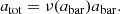
Methods. We estimated the observed intrinsic acceleration (atot) and the baryonic acceleration (abar) from a disk-halo decomposition that incorporates stellar, gas, and dark matter components, with corrections for pressure support, using 3D forward modelling.
Results. We find a RAR in our intermediate-z sample offset from the local relation, with a higher characteristic acceleration scale (a0|z∼1 = 2.38+0.12−0.10 × 10⁻¹⁰ m/s2) and a larger intrinsic scatter (∼0.17 dex). Dividing the sample into redshift bins and refitting the RAR in each bin, we find a characteristic acceleration scale that systematically increases with z. Parametrising the z-dependence as a0(z) = a0(0)+a1 ⋅ z, we obtain a1 = 1.59+0.11−0.10 × 10⁻¹⁰ m/s2, providing evidence for a z-evolution. We find similar results using various dark matter halo profiles as well as the modified Newtonian dynamics framework in our 3D forward modelling.
Conclusions. Our results show that the RAR persists at intermediate redshifts, with statistically significant redshift evolution of the characteristic acceleration, pointing to a possible evolution of the baryon-missing mass connection over cosmic time.
Key words: galaxies: evolution / galaxies: high-redshift / galaxies: kinematics and dynamics
© The Authors 2026
 Open Access article, published by EDP Sciences, under the terms of the Creative Commons Attribution License (https://creativecommons.org/licenses/by/4.0), which permits unrestricted use, distribution, and reproduction in any medium, provided the original work is properly cited.
This article is published in open access under the Subscribe to Open model. This email address is being protected from spambots. You need JavaScript enabled to view it. to support open access publication.
1. Introduction
The missing mass problem in galaxies has been studied since the 1930s (Babcock 1939), but gained prominence in the second half of the 20th century (van de Hulst et al. 1957), especially since the 1970s thanks to observations of flat rotation curves (RCs) in disk galaxies (e.g. Rubin & Ford 1970; Bosma 1978) that deviated from the expected Keplerian decline. This mass discrepancy (Mtot/Mbar ∼ vobs2/vbar2 ≫ 1, where vobs and vbar are the circular velocities, respectively observed and generated by the baryonic content of the galaxy) led to the hypothesis of dark matter (DM) halos surrounding galaxies (e.g. White & Rees 1978; see also reviews such as Bullock & Boylan-Kolchin 2017; Bosma 2023).
This problem was later also quantified in terms of the local radial acceleration in galaxies (Sanders 1990; McGaugh 2004), which led to the identification of the apparently fundamental radial acceleration relation (RAR; McGaugh et al. 2016; Lelli et al. 2017; Stiskalek & Desmond 2023) that connects the observed acceleration (atot = vobs2/r = |∂Φtot(r)/∂r|) to the gravitational acceleration generated by the baryons (abar = vbar2/r = |∂Φbar(r)/∂r|) across all radii. The RAR has been empirically calibrated using the SPARC sample (Lelli et al. 2016), and is usually parametrised by the following relation (McGaugh 2008; Famaey & McGaugh 2012):
 (1)
(1)
This relation exhibits a scatter of ∼0.11 dex (McGaugh et al. 2016), with a characteristic acceleration scale of a0 = 1.2 ± 0.26 × 10⁻¹⁰ m/s2, below which abar begins to deviate systematically from atot. Desmond (2023) and Desmond et al. (2024) refined this analysis on the SPARC sample, and found an even lower intrinsic scatter: σintrinsic = 0.034 ± 0.001stat ± 0.001sys dex.
A few numerical studies have shown that a relation resembling the RAR can occur in the Lambda cold dark matter (ΛCDM) framework using hydrodynamical simulations (Keller & Wadsley 2017; Garaldi et al. 2018; Tenneti et al. 2018; Dutton et al. 2019; Mayer et al. 2023) and semi-empirical analytic models (van den Bosch & Dalcanton 2000; Di Cintio & Lelli 2016; Navarro et al. 1997; Grudić et al. 2020; Paranjape & Sheth 2012; Li et al. 2022). Nevertheless, the detailed results of these studies differ slightly from each other, so that it remains unclear whether some of them do actually reproduce in detail the properties of the observed RAR, including its functional form, very low scatter, and the full diversity of RC shapes to which it applies (Ghari et al. 2019; Desmond 2017).
Alternatively, the RAR may reflect a modification of gravity (or, more generally, of dynamics) rather than unseen matter, which would naturally lead to a very small scatter of the relation. Modified Newtonian dynamics (MOND; Milgrom 1983a,b,c; see also Famaey & Durakovic 2026 for a recent review) introduced a characteristic acceleration scale a0 ∼ 10−10 m/s−2, below which Newtonian dynamics break down. Remarkably, MOND predicted the existence and shape of the RAR decades before it was empirically established.
In the standard MOND framework, a0 is typically considered a universal constant. However, since MOND is a non-relativistic theory, extending it to a cosmological context requires additional assumptions (e.g. Bekenstein 2004; Famaey & McGaugh 2012; Milgrom 2020; Blanchet & Skordis 2024). As a result, there is no clear consensus on whether a0 should remain constant or evolve with cosmic time in the MOND framework. For example, some studies consider a0 as a constant parameter, while others propose that it might scale with the Hubble parameter, H(z), or follow alternative evolutionary paths (e.g. Hossenfelder & Mistele 2018; Maeder 2023; Del Popolo & Chan 2024; Gueorguiev 2024).
In contrast, within ΛCDM, it remains unclear whether the RAR can be fully reproduced as it would have to arise from the complex interplay between baryonic and DM distributions, and any z-evolution of the relation would then reflect the evolving properties of these components. In any case, the degree of z-evolution of a0 in hydrodynamical simulations remains uncertain (e.g. Garaldi et al. 2018; Tenneti et al. 2018; Mayer et al. 2023), likely due to differences in the feedback models used.
While these theoretical frameworks offer different perspectives on the redshift evolution of the RAR, observational studies beyond z = 0 remain scarce, except for Vărăşteanu et al. (2025), who investigated the RAR up to z ∼ 0.08 and found a larger a0 value than at z = 0. For this letter, we studied the RAR at intermediate redshifts up to z ∼ 1.44, offering new insights into the evolution of a0 over cosmic time. This analysis is based on the results presented in Ciocan et al. (2026, hereafter Paper I), where we conducted a disk–halo decomposition using GALPAK3D (Bouché et al. 2015) on a large sample of star-forming galaxies (SFGs), using deep data from the MUSE Hubble Ultra Deep Field survey (MHUDF, Bacon et al. 2023) offering high signal-to-noise (S/N) data ranging from S/N ∼ 10 to > 100.
2. Sample selection and methodology
To investigate the RAR at intermediate z, we selected from the parent sample in Paper I, 79 SFGs with M★ > 108.8 M⊙. This sample has the same minimum stellar mass (i.e. is mass-complete) over 0.33 < z < 1.44 and is part of the MHUDF (Bacon et al. 2023); further details are provided in Appendix A.
In Paper I we performed a detailed 3D disk–halo decomposition on the parent sample of SFGs presented in Fig. A.1, and tested six different DM halo profiles. For the present study, we used the generalised profile of Di Cintio et al. (2014, hereafter DC14) since they provided the best fits compared to other halo models, including the Navarro-Frenk-White (NFW; Navarro et al. 1997) profile. We note that Di Cintio & Lelli (2016) showed that the RAR is more readily reproduced in models with mass-dependent DM density profiles (DC14) than with universal NFW profiles, which struggle to match the observed shape of the relation, particularly in low-M★ galaxies.
We computed abar and atot from the best-fitting DC14 disk–halo models, propagating uncertainties from the Markov chain Monte Carlo (MCMC)-derived velocity components. To minimise resolution-driven biases, measurements within r < 2 kpc (corresponding to approximately one spatial resolution element, i.e. ∼0.2″) were excluded (see Appendix B).
While our analysis relies on parametric modelling, we performed independent consistency checks of the disk–halo decomposition in Paper I, and found consistent results. Additionally, we assessed potential systematic uncertainties in the stellar mass estimates by deriving stellar mass-to-light ratios for our sample. As discussed in Appendix C, these are lower than those assumed at z = 0 in SPARC, but fully consistent with the expected decrease with z from independent studies (Drory et al. 2004).
3. Results
3.1. RAR at 0.33 < z < 1.44
Figure 1 presents the RAR at 0.33 < z < 1.44, using data points from 79 individual model RCs. As illustrated, the RAR at intermediate z is reminiscent of the RAR observed at z = 0 (McGaugh et al. 2016). Our sample, unlike SPARC, predominantly probes the low-acceleration regime as it is largely composed of low-mass, DM-dominated SFGs lacking prominent bulges.
 |
Fig. 1. RAR for the MHUDF sample. The purple curve shows the best-fit RAR at 0.33 < z < 1.44 using Eq. (1), while the red and green curves show the McGaugh et al. (2016) relation at z = 0 and the Vărăşteanu et al. (2025) relation at z < 0.08, respectively. The black dotted line indicates the 1:1 relation. The histogram in the inset displays the residuals with respect to our fit. The cross in the upper left corner indicates the mean 1σ uncertainties. |
We fit the data with Eq. (1), leaving a0 as a free parameter. For the fits, we used the Python package Roxy (Bartlett & Desmond 2023), which implements the marginalised normal regression (MNR) method. This approach simultaneously accounts for uncertainties in both x and y, as well as for the intrinsic scatter in the relation. We applied the MNR to the accelerations in base 10 logarithmic space, and we adopted a uniform broad prior on log a0, ranging from −15 to 5, and on the intrinsic scatter between 0 and 3 dex. We show the best-fit curve in purple in Fig. 1, and as the purple data point in Fig. 2, which corresponds to a characteristic acceleration scale of
 (2)
(2)
 |
Fig. 2. Best-fit a0 values obtained by fitting Eq. (1) on the full sample, using the resolved RAR tracks derived under different modelling assumptions. The purple data point shows a0|z ∼ 1 obtained using the DC14 halo profile applied uniformly to the full sample (Sect. 3.1). The cyan point shows a0|z ∼ 1 derived from a galaxy-by-galaxy best-fitting ΛCDM model, where each galaxy is assigned the DM profile that maximises its Bayesian evidence (Appendix D). The blue point shows a0|z ∼ 1 recovered from the MOND-based framework (Appendix E). The red star indicates the fiducial a0|z ∼ 0 from McGaugh et al. (2016), while the green star shows the result from Vărăşteanu et al. (2025). |
with the errors denoting the 95% confidence intervals (CI) from our MCMC fits. This value is significantly higher, by ∼19σ, than the canonical value of a0|z = 0 = 1.2 ± 0.26 × 10⁻¹⁰ m/s2 inferred for the SPARC sample (McGaugh et al. 2016, shown as the red curve in Fig. 1, and as the red star in Fig. 2), and ∼5σ higher than the value of a0|z < 0.08 = 1.69 ± 0.13 × 10⁻¹⁰ m/s2 inferred by Vărăşteanu et al. (2025) for the MIGHTEE-HI sample (shown as the green curve in Fig. 1, and as the green star in Fig. 2). At face value, this would imply that disks are more submaximal at higher z than at z = 0 in agreement with the large DM fractions found in Paper I.
The histogram in the inset of Fig. 1 shows the residuals with respect to the best-fit RAR at 0.33 < z < 1.44, which are tightly peaked, with a mean offset of μ = 0.016 dex and a standard deviation of σ = 0.19 dex, similar to the intrinsic scatter (σintr. ∼ 0.17 dex). The scatter that we recover for the intermediate-z sample is ∼ × 1.5 higher than that inferred by McGaugh et al. (2016) for the SPARC sample, which is of the order of ∼0.11 dex. The larger scatter that we measure is most likely related to the broad z range that we probed, as discussed in the next section, and to the poorer data quality at higher z.
As mentioned above, our analysis relies on the parametric models from Paper I, where we found that the DC14 density profile provides the best representation of the data. To assess the robustness of our results, we explored alternative DM profiles (see Appendix D) and also refitted the data within a self-consistent MOND framework (see Appendix E). The resulting a0|z ∼ 1 values from these various assumptions are always larger than the z = 0 value and agree within the errors with the results presented above, as shown in Fig. 2 by the cyan and blue data points.
3.2. Evolution of the RAR with z
To carefully trace the potential evolution of the RAR with cosmic time, we applied a quantile-based binning of the galaxy redshift distribution. Specifically, we divided the sample into four quantile intervals containing approximately the same number of data points and, for each interval, we fit the RAR with Eq. (1) to extract the best-fit characteristic acceleration scale. The fits were performed following the same procedure as in Sect. 3.1. We adopted this equal-population binning to stabilise the Bayesian fits by ensuring comparable statistical weight in each bin; we note that the bins correspond to adjacent, non-overlapping z intervals.
We show the resulting a0(z) values in Fig. 3 as the black data points. As illustrated, the characteristic acceleration systematically increases with redshift, rising from ∼1.99 × 10⁻¹⁰ m/s2 in the lowest-z bin to 2.71 × 10⁻¹⁰ m/s2 in the highest.
 |
Fig. 3. Redshift evolution of the characteristic acceleration scale. In each quantile-based z bin (blue bars), we fit the RAR with Eq. (1) to derive a0, with uncertainties shown as grey error bars. The star marks the SPARC z = 0 value. The purple line shows the predicted evolution, using the best-fitting parameters from the global z-dependent fit to the RAR for the full sample (i.e. using Eq. (1) where a0 was substituted with Eq. (3); see Eq. (4)). The red line shows the same, but including SPARC in the fit. The coloured shaded region shows the 1σ errors for the fits. |
We evaluated the intrinsic scatter in each redshift bin and found an increase with z, from σintr. = 0.13 dex in the lowest-redshift bin–below the full-sample value–to σintr. = 0.19 dex in the highest. Nevertheless, the scatter in the individual z bins remains larger than that observed in the SPARC sample, likely reflecting the degradation in data quality and spatial resolution with increasing z, and the lower statistics.
To complement this binned analysis, we also performed a global parametric fit to quantify the z-dependence of the RAR by introducing a z-dependent acceleration scale of the form
 (3)
(3)
where the coefficient a1 captures the evolutionary trend with z, following the approach of Vărăşteanu et al. (2025). We then refit the RAR for the entire sample using Eq. (1), where we substitute a0 with the z-dependent formulation (Eq. (3)), treating both a0(0) and a1 as free parameters in the fits. We obtain
 (4)
(4)
with the errors denoting the 95% CI. We note that including the SPARC sample (Lelli et al. 2017) in the fits yields similar results.
We show this linear relation, using the best-fit values of a0(0) and a1 from the fit to the MHUDF RAR (Fig. 1) as the purple line in Fig. 3. The red line shows the same, but with the SPARC sample included in the fit. In Appendix F we present the resulting posterior distributions of the fitted parameters, and discuss the small offsets between the binned estimates and the global fit.
We emphasise that this linear parametrisation of a0(z) (Eq. (3)) is intended as a simple phenomenological description to quantify the presence and sign of a possible z-dependence rather than to provide a physically motivated description. If the real z-dependence of a0 is non-linear or more complex, the resulting evolutionary trend could be affected by systematic biases.
In conclusion, the results presented in this section suggest that while the RAR persists out to z ∼ 1.44, the value of a0 increases with z, potentially reflecting changes in the baryon–DM coupling, in the feedback efficiency, or in modified gravity over cosmic time.
4. Discussion
The results presented above indicate that the RAR evolves with z. We quantified this evolution with a simple, linear model (Eq. (3)), obtaining  . Our result can be compared to the z ≤ 0.08 study of Vărăşteanu et al. (2025), who found a1 = (4.47 ± 1.88) × 10−10 m s−2 from a smaller sample. While their analysis provided only mild evidence (∼ 2.4σ) for a z-evolution, our broader z-baseline and larger sample yield a more statistically significant detection (at a ∼30σ level). The two measurements are statistically consistent within ∼ 1.5σ.
In the context of ΛCDM, our results show a roughly comparable z-trend as reported by Mayer et al. (2023) and Keller & Wadsley (2017), although the robustness of some of these results to reproduce the observed low-z RAR has been questioned (Milgrom 2016). For example, Mayer et al. (2023) find that a0 grows by a factor of ∼3 from z = 0 to 2, slightly less than the factor of ∼4 increase inferred here over the same z range. In the context of modified gravity, our measured a0(z) is faster than that of H(z) (Milgrom 1983a), and is in tension with the evolution predicted by the scale invariant vacuum paradigm (Gueorguiev 2024).
An evolution of the RAR with z should be reflected in the baryonic Tully–Fisher relation (bTFR). Current bTFR measurements based on H I detections at z ≲ 0.4 (Ponomareva et al. 2021; Jarvis et al. 2025) show little to no evidence for evolution, but are limited by small samples, narrow z baselines, and large uncertainties. Our z-dependent RAR fit (Eq. (4)) predicts a bTFR zero-point shift of ΔZP ≈ −0.2 dex between z ∼ 0 and z ∼ 1. At higher z, Übler et al. (2017) find a decrease in the bTFR zero-point between z ∼ 0 and z ∼ 0.9 (ΔZP = −0.44), though their Mbar estimates rely on scaling relations and neglect MH I, while Jeanneau et al. (2026) found no evolution of the bTFR at z ∼ 1, accounting for neutral gas from scaling relations. Looking ahead, deep H I surveys with the Square Kilometre Array will provide critical tests of the potential evolution of both the bTFR and the RAR with z.
5. Conclusions
In this study we analysed the RAR at intermediate redshifts (0.33 < z < 1.44), for a mass-complete sample of 79 SFGs with 8.8 < log(M★/M⊙) < 11, using 3D forward modelling. To do so, we used the results obtained in Paper I from the disk–halo decomposition. Our analysis has yielded several key findings:
-
The RAR for our z ∼ 1 sample exhibits a higher acceleration scale
 compared to the canonical value inferred by McGaugh et al. (2016) for the z = 0 SPARC sample (Fig. 1).
 -
A larger value of a0|z ∼ 1 is found regardless of the model used to derive the total and the baryonic accelerations (Fig. 2), including various ΛCDM and MOND models for self-consistency (Appendices D and E).
-
By fitting Eq. (1) independently in four redshift bins, we recover a systematic increase of the best-fit a0 with z (Fig. 3).
-
Fitting Eq. (1) to the full sample by substituting a0 with the redshift-dependent formulation, a0(z) = a0(0)+a1 ⋅ z, yields
 , providing evidence for an increase in a0 with redshift (Figs. 3 and F.1).
Some hydrodynamical simulations and modified-gravity frameworks predict a possible redshift evolution of a0, although the magnitude and functional form vary across models. At present, theoretical expectations remain too diverse to make definitive comparisons. Our results, therefore, motivate future efforts to refine predictive models and explore the physical mechanisms that could shape any evolution of the RAR with cosmic time.
Acknowledgments
We thank the anonymous referee for constructive comments that improved the manuscript. JFr acknowledges stimulating discussions on the topic with S. Trujillo-Gomez. This work is based on observations collected under ESO programmes 094.A-0289(B), 095.A-0010(A), 096.A-0045(A), 096.A-0045(B) and 1101.A-0127. This research made use of the following open source software: Astropy (Robitaille et al. 2013), numpy (van der Walt et al. 2011) and matplotlib (Hunter 2007). BC, NB and JFe acknowledge support from the ANR DARK grant (ANR-22-CE31-0006). HD is supported by the Royal Society University Research Fellowship grant 211046.
References
- Babcock, H. W. 1939, Lick Obs. Bull., 498, 41 [Google Scholar]
- Bacon, R., Brinchmann, J., Conseil, S., et al. 2023, A&A, 670, A4 [NASA ADS] [CrossRef] [EDP Sciences] [Google Scholar]
- Bartlett, D. J., & Desmond, H. 2023, Open J. Astrophys., 6, 42 [Google Scholar]
- Bekenstein, J. D. 2004, Phys. Rev. D, 70, 083509 [Google Scholar]
- Blanchet, L., & Skordis, C. 2024, JCAP, 2024, 040 [Google Scholar]
- Bosma, A. 1978, Ph.D. Thesis, University of Groningen, Netherlands [Google Scholar]
- Bosma, A. 2023, ArXiv e-prints [arXiv:2309.06390] [Google Scholar]
- Bouché, N., Carfantan, H., Schroetter, I., et al. 2015, AJ, 150, 92 [CrossRef] [Google Scholar]
- Bullock, J. S., & Boylan-Kolchin, M. 2017, ARA&A, 55, 343 [Google Scholar]
- Burkert, A. 1995, ApJ, 447, L25 [NASA ADS] [Google Scholar]
- Casertano, S. 1983, MNRAS, 203, 735 [NASA ADS] [CrossRef] [Google Scholar]
- Ciocan, B. I., Bouché, N. F., Fensch, J., et al. 2026, A&A, 708, A112 [NASA ADS] [CrossRef] [EDP Sciences] [Google Scholar]
- Dalcanton, J. J., & Stilp, A. M. 2010, ApJ, 721, 547 [NASA ADS] [CrossRef] [Google Scholar]
- Del Popolo, A., & Chan, M. H. 2024, Phys. Dark Universe, 43, 101415 [Google Scholar]
- Desmond, H. 2017, MNRAS, 464, 4160 [Google Scholar]
- Desmond, H. 2023, MNRAS, 526, 3342 [NASA ADS] [CrossRef] [Google Scholar]
- Desmond, H., Hees, A., & Famaey, B. 2024, MNRAS, 530, 1781 [Google Scholar]
- Di Cintio, A., & Lelli, F. 2016, MNRAS, 456, L127 [NASA ADS] [CrossRef] [Google Scholar]
- Di Cintio, A., Brook, C. B., Dutton, A. A., et al. 2014, MNRAS, 441, 2986 [Google Scholar]
- Drory, N., Bender, R., Feulner, G., et al. 2004, ApJ, 608, 742 [Google Scholar]
- Dutton, A. A., Macciò, A. V., Obreja, A., & Buck, T. 2019, MNRAS, 485, 1886 [NASA ADS] [CrossRef] [Google Scholar]
- Emsellem, E., Monnet, G., & Bacon, R. 1994, A&A, 285, 723 [NASA ADS] [Google Scholar]
- Epinat, B., Tasca, L., Amram, P., et al. 2012, A&A, 539, A92 [NASA ADS] [CrossRef] [EDP Sciences] [Google Scholar]
- Famaey, B., & Durakovic, A. 2026, Encyclopedia of Astrophysics, Volume 5, 121 [Google Scholar]
- Famaey, B., & McGaugh, S. 2012, Liv. Rev. Relativ., 15, 10 [Google Scholar]
- Freundlich, J., Combes, F., Tacconi, L. J., et al. 2019, A&A, 622, A105 [NASA ADS] [CrossRef] [EDP Sciences] [Google Scholar]
- Freundlich, J., Jiang, F., Dekel, A., et al. 2020, MNRAS, 499, 2912 [NASA ADS] [CrossRef] [Google Scholar]
- Garaldi, E., Romano-Díaz, E., Porciani, C., & Pawlowski, M. S. 2018, Phys. Rev. Lett., 120, 261301 [Google Scholar]
- Ghari, A., Famaey, B., Laporte, C., & Haghi, H. 2019, A&A, 623, A123 [NASA ADS] [CrossRef] [EDP Sciences] [Google Scholar]
- Grudić, M. Y., Boylan-Kolchin, M., Faucher-Giguère, C.-A., & Hopkins, P. F. 2020, MNRAS, 496, L127 [CrossRef] [Google Scholar]
- Gueorguiev, V. G. 2024, MNRAS, 535, L13 [Google Scholar]
- Hernquist, L. 1990, ApJ, 356, 359 [Google Scholar]
- Hossenfelder, S., & Mistele, T. 2018, Int. J. Mod. Phys. D, 27, 1847010 [Google Scholar]
- Hunter, J. D. 2007, Comput. Sci. Eng., 9, 90 [NASA ADS] [CrossRef] [Google Scholar]
- Jarvis, M. J., Tudorache, M. N., Heywood, I., et al. 2025, MNRAS, 544, 193 [Google Scholar]
- Jeanneau, A., Richard, J., Bouché, N. F., et al. 2026, A&A, 709, A120 [NASA ADS] [CrossRef] [EDP Sciences] [Google Scholar]
- Keller, B. W., & Wadsley, J. W. 2017, ApJ, 835, L17 [Google Scholar]
- Lelli, F., McGaugh, S. S., & Schombert, J. M. 2016, AJ, 152, 157 [Google Scholar]
- Lelli, F., McGaugh, S. S., Schombert, J. M., & Pawlowski, M. S. 2017, ApJ, 836, 152 [Google Scholar]
- Li, P., McGaugh, S., Lelli, F., et al. 2022, ApJ, 927, 198 [NASA ADS] [CrossRef] [Google Scholar]
- Maeder, A. 2023, MNRAS, 520, 1447 [Google Scholar]
- Mayer, A., Teklu, A. F., Dolag, K., & Remus, R.-S. 2023, MNRAS, 518, 257 [Google Scholar]
- McGaugh, S. S. 2004, ApJ, 609, 652 [NASA ADS] [CrossRef] [Google Scholar]
- McGaugh, S. S. 2008, ApJ, 683, 137 [NASA ADS] [CrossRef] [Google Scholar]
- McGaugh, S. S., Lelli, F., & Schombert, J. M. 2016, Phys. Rev. Lett., 117, 201101 [NASA ADS] [CrossRef] [Google Scholar]
- McGaugh, S. S., Li, P., Lelli, F., & Schombert, J. M. 2018, Nat. Astron., 2, 924 [Google Scholar]
- Milgrom, M. 1983a, ApJ, 270, 365 [Google Scholar]
- Milgrom, M. 1983b, ApJ, 270, 371 [Google Scholar]
- Milgrom, M. 1983c, ApJ, 270, 384 [Google Scholar]
- Milgrom, M. 2016, ArXiv e-prints [arXiv:1610.07538] [Google Scholar]
- Milgrom, M. 2020, ArXiv e-prints [arXiv:2001.09729] [Google Scholar]
- Navarro, J. F., Frenk, C. S., & White, S. D. M. 1997, ApJ, 490, 493 [Google Scholar]
- Navarro, J. F., Hayashi, E., Power, C., et al. 2004, MNRAS, 349, 1039 [Google Scholar]
- Paranjape, A., & Sheth, R. K. 2012, MNRAS, 426, 2789 [Google Scholar]
- Ponomareva, A. A., Mulaudzi, W., Maddox, N., et al. 2021, MNRAS, 508, 1195 [NASA ADS] [Google Scholar]
- Read, J. I., Agertz, O., & Collins, M. L. M. 2016, MNRAS, 459, 2573 [NASA ADS] [CrossRef] [Google Scholar]
- Robitaille, T. P., Tollerud, E. J., Greenfield, P., et al. 2013, A&A, 558, A33 [NASA ADS] [CrossRef] [EDP Sciences] [Google Scholar]
- Rodrigues, D. C., Marra, V., del Popolo, A., & Davari, Z. 2018, Nat. Astron., 2, 668 [Google Scholar]
- Rubin, V. C., & Ford, W. K. 1970, ApJ, 159, 379 [NASA ADS] [CrossRef] [Google Scholar]
- Sanders, R. H. 1990, A&ARv, 2, 1 [NASA ADS] [CrossRef] [Google Scholar]
- Stiskalek, R., & Desmond, H. 2023, MNRAS, 525, 6130 [NASA ADS] [CrossRef] [Google Scholar]
- Tenneti, A., Di Matteo, T., Croft, R., et al. 2018, MNRAS, 474, 597 [Google Scholar]
- Übler, H., Förster Schreiber, N. M., Genzel, R., et al. 2017, ApJ, 842, 121 [Google Scholar]
- van de Hulst, H. C., Raimond, E., & van Woerden, H. 1957, Bull. Astron. Inst. Netherlands, 14, 1 [Google Scholar]
- van den Bosch, F. C., & Dalcanton, J. J. 2000, ApJ, 534, 146 [Google Scholar]
- van der Walt, S., Colbert, S. C., & Varoquaux, G. 2011, Comput. Sci. Eng., 13, 22 [Google Scholar]
- Vărăşteanu, A. A., Jarvis, M. J., Ponomareva, A. A., et al. 2025, MNRAS, 541, 2366 [Google Scholar]
- White, S. D. M., & Rees, M. J. 1978, MNRAS, 183, 341 [Google Scholar]
We rescaled the evidence log(𝒵) by a factor of -2 so that it is on the same scale as the usual information criterion; in this convention, lower values correspond to better-fitting models.
For the 4 galaxies in this sample which have a bulge-to-total ratio B/T > 0.2, a bulge component is included in the disk–halo decomposition.
The MOND prescription used here is in isolation, without accounting for the external field effect (EFE), which arises when a system is subject to a constant external gravitational field. Since our sample excludes interacting galaxies and cluster members, the EFE is expected to have only a minor impact.
We fitted our data with MOND models in which the δ parameter was fixed to δ = 1 or δ = 2.5, or allowed to vary with broad Gaussian priors, all of which yielded very similar results for our sample.
Appendix A: Sample of intermediate-z SFGs
For this study, we used the sample of SFGs with RC decomposition from Paper I, which are drawn from the MHUDF survey (Bacon et al. 2023). A comprehensive description of the initial sample selection is provided in Paper I; here we briefly summarise the key criteria. The parent sample consists of intermediate-z SFGs with high S/N (∼10 to > 100) in either [O II] λ3727, Hβ, [O III] λ5007, Hα, which are well resolved, have inclinations i > 30°, are rotationally supported (vmax/σ > 1), and show no evidence for ongoing mergers. For the present analysis, we further restrict the sample to galaxies classified as ‘regular’ in Paper I. This classification was based on a visual inspection of rest-frame optical/IR morphologies and kinematic maps, selecting systems showing no obvious signs of gravitational interactions (e.g. tidal features, asymmetries, or disturbed velocity fields). In addition, we only selected galaxies that exhibit small residuals in the kinematic modelling, i.e. which have good fits, quantified by log(𝒵) < 15000, where log(𝒵) is the model evidence.1
To robustly investigate the redshift evolution of the RAR, it is crucial to work with a sample defined by a uniform stellar-mass distribution across the redshift range considered, i.e. imposing the same minimum M★ at all redshifts. Figure A.1 indicates that the MHUDF survey is complete down to a stellar-mass of log(M★/M⊙) = 8.6 over 0.2 < z < 1.44, whereas the sample from Paper I is complete to log(M★/M⊙) = 8.8 due to the additional S/N criteria that were imposed. We therefore adopt a stellar-mass cut of log(M★/M⊙) > 8.8, yielding a final sample of 79 SFGs (blue-red data points in Fig. A.1) used in this study. These galaxies span stellar masses and redshifts in the ranges 8.8 < log(M★/M⊙) < 11 and 0.33 < z < 1.44, respectively.
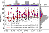 |
Fig. A.1. Stellar masses vs redshift for all MHUDF SFGs. The dashed black line indicates the mass completeness limit of the survey, which is reasonably complete for 0.2 < z < 1.5 down to log(M★/M⊙) = 8.6. The dashed red line shows the completeness of the parent sample from Paper I. The grey points show all SFGs observed in the MHUDF survey, the red-outlined points correspond to the galaxies analysed in Paper I, and the blue points indicate the galaxies studied in this work. The histograms on the top and right display the redshift and stellar-mass distributions, respectively, colour-coded to match the main panel. |
Appendix B: Methodology
Based on the disk-halo decomposition from Paper I,
 (B.1)
(B.1)
we calculated the baryonic acceleration due to the baryonic mass distribution at every radius as
 (B.2)
(B.2)
and the total acceleration as
 (B.3)
(B.3)
Here vdisk(r), vHI(r), and vbulge(r) denote the contributions of the stellar disk, neutral atomic gas, and bulge2 to the RC, respectively, while vDM(r) represents the contribution of the DM halo. The circular velocity, vc(r), is corrected for pressure support (asymmetric drift) following Dalcanton & Stilp (2010), such that vc2(r) = v⊥2(r)+vAD2(r), where v⊥(r) is the observed rotation velocity and vAD(r) is the pressure support correction. We note that all velocity terms are intrinsic, i.e. corrected for any instrumental effects, including seeing.
We briefly summarise here the main ingredients of the 3D disk–halo decomposition (see Paper I for full details). The DM halo was parametrised using the best-fitting DM density profile from Paper I, namely DC14 (Di Cintio et al. 2014). For the neutral gas component, we used a parametric model which assumes a constant H I surface mass density, leading to  . The bulge, if present, was modelled as a Hernquist (1990) spheroidal component. The disk contribution was parametrised from the observed ionised gas surface brightness profiles using a Multi-Gaussian Expansion modelling (Emsellem et al. 1994), whereas the normalisation of vdisk(r) was given by M★. Importantly, M★ itself was not fixed by photometric priors. Instead, it was dynamically inferred in our 3D forward modelling. Within the DC14 framework, the disk-halo degeneracy is mitigated by fitting for log(M★/Mhalo) together with the virial velocity. This allows the stellar mass to be constrained directly by the kinematics.
For illustration, we show in Fig. B.1 the 3D disk–halo decomposition for two galaxies from our sample. We note that all catalogues and data products from our disk–halo decomposition, including the RCs, can be found on the DARK website.3 For MXDF 1266 (left, M★,SED = 109.05 M⊙), the RC is dominated by the DM component, indicating a strongly submaximal disk compared to local higher-mass spirals (e.g. Lelli et al. 2016). On average, we find that most of our sample has DM fractions larger than 50% within Re (i.e. they are submaximal), as shown in Paper I. In contrast, the higher-mass galaxy, MOSAIC 905 (right, M★,SED = 1010.3 M⊙), is dominated by the stellar component within 2Re.
 |
Fig. B.1. Examples of the 3D disk-halo decomposition for the two galaxies from the sample. The solid black line represents the circular velocity vc(r) corrected for pressure support. The solid green curve represents the RC of the DM component. The solid orange and blue curves represent the disk and cold gas components, respectively. The light shaded regions show the 95% CI. The dotted brown line represents the stellar component measured using the multi-Gaussian expansion modelling of resolved stellar mass maps obtained from pixel-by-pixel SED fitting, while the dash-dotted green curve shows the DM component obtained independently from a 1D disk–halo decomposition. All velocities are intrinsic, i.e. corrected for inclination and instrumental effects, including seeing (PSF). The black dotted line shows the physical extent of a MUSE spaxel. |
The 1σ errors in the velocity components were derived from the 68% CI of the MCMC chains. Specifically, for each model parameter, we computed the 16th and 84th percentiles of the posterior distributions, providing the lower and upper bounds of the CI. To estimate the uncertainties in the baryonic and total accelerations, we propagated the errors from the velocity components using standard error propagation techniques.
To minimise the impact of observational uncertainties, particularly in regions where the rotation and acceleration profiles are poorly resolved, we excluded measurements in the innermost regions (r < 2 kpc) from the final fits to the RAR. Due to the finite spatial resolution of the MUSE instrument (0.2″spaxels, black dotted lines in Fig. B.1), measurements in these innermost regions are affected by resolution limitations that might bias our final results. A similar approach was taken in Vărăşteanu et al. (2025). We note, however, that excluding measurements within the central 2 kpc for both the MHUDF and SPARC (Lelli et al. 2017) samples changes the inferred a0 by less than 10%.
Appendix C: Robustness tests and systematic uncertainties on disk masses
In this appendix, we assess the robustness of our results with respect to the main modelling assumptions. We emphasise that our measurement of the RAR at intermediate z is not strictly identical to the traditional local-Universe approach, as it relies on 3D forward modelling. While this technique represents the state of the art for intermediate- to high-z galaxy dynamics, it necessarily introduces a degree of model dependence, stemming from assumptions about the halo profile, disk geometry and gas distribution, among other factors. In this framework, both the total acceleration, atot(r), and the baryonic acceleration, abar(r), are derived from the same underlying model rather than independently, as is typically done at z ∼ 0.
Nonetheless, we note that in Paper I, we presented a series of consistency checks supporting the robustness of our disk–halo decomposition. Specifically: (i) The total circular velocity, vc(r), was independently measured using the traditional 2D line-fitting algorithm CAMEL (Epinat et al. 2012), yielding results in good agreement with those obtained from the 3D parametric modelling (rendering vc(r) effectively model-independent). (ii) The stellar disk contribution, vdisk(r), was independently derived via a Multi-Gaussian Expansion (Emsellem et al. 1994) modelling applied to resolved stellar-mass maps obtained from pixel-by-pixel SED fitting across ∼ 19 Hubble Space Telescope and James Webb Space Telescope bands, again showing good agreement (as illustrated by the brown dotted curves in Fig. B.1). (iii) For the unknown neutral gas contribution, vHI(r), we explored a range of plausible H I surface-density profiles–given their lack of direct constraints–and found that our results are consistent across various assumed profile shapes. (iv) Finally, we performed a fully independent 1D disk–halo decomposition by computing the baryonic contribution to the RC. This was achieved by solving the Poisson equation for the surface-density distribution of the stellar and cold gas components (i.e. by solving Eq. 4 of Casertano 1983). This 1D approach yielded results consistent with those from the 3D modelling (as illustrated by the green dash-dotted curves in Fig. B.1).
Given the central role of M★ in our results, it is important to note the dynamically inferred stellar masses are in good agreement with independent SED-based estimates (Fig. 11 of Paper I), showing that the potential systematic uncertainties in M★ are negligible. In addition, we computed the rest-frame K-band mass-to-light ratios (M/LK) of our sample, using photometric data from the Hubble Space Telescope and James Webb Space Telescope (see Paper I), and compared them to independent measurements at similar redshifts from Drory et al. (2004). Figure C.1(left) shows that the M/LK of our sample are fully consistent with typical values reported at higher redshifts accounting for the mass dependence, and are systematically lower than those adopted for SPARC at z = 0, which have M/LK ∼ 0.6 in the K-band (corresponding to M/L ∼ 0.5 at 3.6 μm, McGaugh et al. 2016).
 |
Fig. C.1. Left: Average mass-to-light ratios (M/L) in the K-band as a function of redshift for the MHUDF sample split into two M★ bins, the low-M★ bin (yellow) and high-M★ bin (orange), along with the evolution inferred for a sample of more than 5000 K-selected galaxies in Drory et al. (2004). The red star shows the M/L-K ratio adopted for the SPARC sample. Right: Impact of systematic disk mass offsets on the inferred a0(z). The black points correspond to the fiducial fits shown in Fig 3. The blue points show the inferred a0(z) assuming a global shift of +0.2 dex in the mass budget of the sample, while the green points show the same, but when assuming a global shift of +0.45 dex . The red star and dotted lines show the canonical a0(z = 0) inferred for the SPARC sample. |
To further assess the impact of systematic uncertainties in the disk mass estimates on the RAR, we also explore how global systematic shifts in the M★ would affect the inferred a0(z). Specifically, we recompute the RAR after applying uniform offsets to M★ across the sample. We find that reconciling our measurements with the canonical value a0(0) = 1.2 × 10⁻¹⁰ m s−2 at all redshifts would require systematically larger stellar masses, with offsets ranging from ∼ + 0.2 dex in the lowest-redshift bins to ∼ + 0.45 dex in the highest (Fig. C.1, right). As argued above and discussed in Paper I, such large shifts are not supported by independent consistency checks.
We note that in order to improve our modelling, direct constraints on the gas components will be required. However, as discussed in Paper I, given typical molecular gas fractions of ∼30-50% at z ∼ 1 (Freundlich et al. 2019), this would introduce a systematic uncertainty of ∼0.2 dex in the total disk mass.
Finally, in Appendices D and E, we explored the RAR from RC decompositions using different parametric models in the ΛCDM and MOND frameworks, respectively, finding consistent results with those presented in the main text. Together, these tests demonstrate that our results are not driven by any single modelling assumption, but instead, most likely, reflect a genuine physical trend.
Appendix D: Robustness tests: RAR from different DM halo models in ΛCDM
To ensure that our conclusions on the redshift evolution of the RAR are not driven by methodological choices, we investigated how variations in our modelling assumptions influence the recovered accelerations abar(r) and atot(r). In Paper I we tested six DM density profiles in our disk–halo decomposition: (1) DC14 (Di Cintio et al. 2014), which links the halo profile shape to the stellar-to-halo mass ratio; (2) NFW (Navarro et al. 1997); (3) Burkert (Burkert 1995; (4) Dekel–Zhao (Freundlich et al. 2020); (5) Einasto (Navarro et al. 2004); and (6) coreNFW (Read et al. 2016). Our analysis showed that DC14 provides the best population-level fit, and we refer to the Bayesian model comparison in Paper I for details.
In this section, we adopted a galaxy-by-galaxy approach: for each system, we selected the profile that yields the best Bayesian evidence in the pairwise comparisons. Each galaxy was therefore assigned its own preferred model (e.g. DC14 for some, NFW for others). Using these best-fitting models for each galaxy, we recomputed abar(r) and atot(r) (as detailed in Appendix B). The resulting RAR tracks are shown as coloured points in Fig. D.1. We then refited the RAR for the full sample (Eq. 1), treating the characteristic acceleration scale as a free parameter (as in Sect. 3.1); the best-fit relation is shown as the purple curve. Additionally, in Fig. 2, we also show the best-fit value of a0|z ∼ 1 obtained in this framework as the cyan data point. We find
 (D.1)
(D.1)
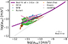 |
Fig. D.1. RAR of our intermediate-z sample, with abar and atot derived from the model RCs corresponding to each galaxy’s best-fitting ΛCDM halo profile. The coloured points indicate the halo profile used in the disk–halo decomposition. The cross in the lower right corner indicates the mean 1σ uncertainties on the data points. The dotted black line shows the 1:1 relation. The purple curve represents the best-fit RAR, with |

a result that is consistent, within the errors, with the value derived in the main text (Eq. 2), where the DC14 profile is applied uniformly to the full sample (purple data point in Fig. 2). Figure 2 illustrates that regardless of the model used to derive the total and the baryonic accelerations, the a0|z ∼ 1 value inferred from the RAR is offset from the z = 0 canonical value.
Following the same procedure presented in Sect. 3.2, we fit the RAR in this framework using the z-dependent acceleration scale (Eq. 1 substituting a0 with Eq. 3), and obtain
 (D.2)
(D.2)
which agrees within 1σ with the results presented in the main text when using DC14 uniformly for the whole sample.
Overall, these tests demonstrate that our results are fairly robust against the choice of DM profile: whether using DC14 uniformly or adopting the best-fitting model for each galaxy individually, the recovered redshift evolution of the RAR remains consistent. In the next section, we discuss the RAR derived from the MOND framework.
Appendix E: Robustness tests: RAR from MOND models
To investigate the RAR in the MOND framework, we first need to refit our MHUDF data directly with MOND parametric models, and then re-analyse the RAR from these new fits as in Sect. 3. To refit our data, we extended our 3D modelling framework, GALPAK3D (Bouché et al. 2015), to MOND (Milgrom 1983a) 4 using the interpolation functions defined in Sect. 3.3 of Famaey & Durakovic (2026). Specifically, we used two interpolation function families (Milgrom 1983c, McGaugh et al. 2016),
![Mathematical equation: $$ \begin{aligned}&\mathrm {n-family}: \nu _n(x) = \left[ \frac{1 + \sqrt{1 + 4 (x / a_0)^{-n}}}{2} \right]^{1/n} and \end{aligned} $$](/articles/aa/full_html/2026/05/aa59230-26/aa59230-26-eq17.gif) (E.1)
(E.1)
 (E.2)
(E.2)
which relate the total and baryonic accelerations as
 (E.3)
(E.3)
Briefly, in our implementation within GALPAK3D, the Newtonian baryonic acceleration abar(r) is computed directly from the disk, gas and, where applicable, bulge parametric models described in Paper I (and briefly detailed in Appendix B, and thus, does not depend on any MOND-specific parameters). The code then evaluates the total acceleration atot(r) using Eq. E.3. Again, corrections for pressure support, following Dalcanton & Stilp (2010), were applied to the RCs.
The free parameters of the model are the same as in Paper I, with the addition of the MOND-specific parameters, namely n or δ, depending on the interpolation function, and the acceleration scale, a0. We adopt the same priors as in Paper I for all shared parameters. For the n-family model (Eq. E.1), we use a flat prior 0.7 < n < 1.3 , while for the δ-family model (Eq. E.2), we use a similar prior: 0.7 < δ < 1.3. These values are motivated by Desmond et al. (2024), who showed that the best fits to galaxy RCs were systematically close to n ∼ 1 or δ ∼ 1. We note that δ = 1 immediately gives back the usual form of Eq. 1.5 We find that the two MOND models (E.1 and E.2) perform similarly well, with a Bayes factor −2 < Δ log(𝒵) < 2, meaning that they are indistinguishable, and we therefore quote results for the δ-family (Eq. E.2, with δ ∼ 1, i.e. effectively Eq. 1) in the remainder of this appendix.
Before discussing the RAR in the MOND framework, we attempted to quantify the redshift evolution of a0(z) from the individual fits to our MUSE data cubes with: (i) a0 free in each galaxy, with a broad flat prior 10−11 < a0 < 10−9; (ii) a0 fixed to the z = 0 canonical value; and (iii) with the redshift evolution a0(z) (Eq. 3), where a1 is a free parameter for each galaxy (with a broad flat prior −1 × 10⁻⁹ < a1 < 1 × 10⁻⁹) and a0(0) is kept fixed to the z = 0 value.
Regarding (i), a0 was treated as a free parameter in the kinematic modelling of the individual MUSE cubes, and we do not recover a single, well-defined characteristic acceleration for the sample. Instead, the inferred a0|z ∼ 1 values display broad galaxy-to-galaxy variations, ranging from 1.3 × 10⁻¹¹ to 9.6 × 10⁻¹⁰ m/s2, with a median value of a0|z ∼ 1 = 2.27 × 10⁻¹⁰ m/s2 (close to the value inferred in the main text in the ΛCDM framework - Eq. 2). It is worth noting that similar results were obtained by Rodrigues et al. (2018), who used Bayesian inference on the SPARC and THINGS samples to show that the probability of a single, universal acceleration scale common to all galaxies is effectively zero (but see also McGaugh et al. (2018) on the role of inclination and M/L uncertainties and priors on this statistical result).
We tested whether the acceleration scales inferred from our fits to the individual data cubes are consistent with being at or below the canonical SPARC value, by performing a one-sided Kolmogorov–Smirnov (KS) test. The fiducial value was modelled as a Gaussian distribution centred on a0 = 1.2 × 10⁻¹⁰ m/s2 with a width equal to the measurement error 0.26 × 10⁻¹⁰ reported in McGaugh et al. (2016). Our measurement uncertainties were incorporated by generating 10000 Monte Carlo realisations of the sample. In every realisation, the null hypothesis is rejected at a confidence level of 99%, with a median statistic of D = 0.55 and a median p − value = 5.5 · 10−20, indicating that the inferred values are systematically higher than the canonical a0(0) value.
Regarding (ii), when a0 is fixed to a0(0) = 1.2 × 10⁻¹⁰ m/s2 in the kinematic modelling, we found that the fits are worse, with the Bayes factor indicating positive evidence (Δlog(𝒵) < −2) for the models with a0 as a free parameter. We find that the model with free a0 (i.e. model i) performs as well or better than that for a fixed a0 (i.e. model ii) for ≳ 70% of the sample. Similar results were obtained when comparing the model with z-varying a0 (i.e. model iii) to the one with fixed a0. We also note that the dynamically inferred M★ using the model with fixed a0 are overestimated by ∼0.28 dex with respect to the ones obtained in the main text using DC14, and are likewise elevated compared to independent SED-based estimates (although it does bring the M/L closer to those assumed in the SPARC database at z = 0).
Regarding (iii), we show the resulting a1 values from the individual fits in Fig. E.1 (solid histogram). This figure reveals that the inferred a1 values are predominantly positive, suggesting a positive correlation between the characteristic acceleration scale and redshift, and that the peak of the a1 distribution is near the value (vertical line) obtained with the z-dependent fit to the RAR discussed in the main text (see Sect. 3.2: Eq. 4, Fig. 3). While individual a1 values carry measurement uncertainties, we quantify the significance of the overall positive trend using a one-sample KS test (described below), which incorporates these uncertainties.
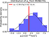 |
Fig. E.1. Distribution of the MOND acceleration parameter a1. The purple histogram shows the recovered a1 values from individual galaxy fits. The vertical red line marks the reference value obtained from the RAR in the main text, |

To quantify the statistical significance of this apparent offset from zero, we tested whether the a1 values are consistent with being drawn from a zero-mean Gaussian distribution. This was achieved by performing a one-sample KS test against a standard normal null cumulative distribution function. Our measurement uncertainties were incorporated by generating 10000 Monte Carlo realisations of the sample. In every realisation, the null hypothesis is rejected at the 99% confidence level, with a median KS statistic of D = 0.30 and a median p-value of 1.2 × 10⁻⁵. This indicates that the distribution of a1 is inconsistent with a zero-mean Gaussian.
Taken together, these results indicate that the individual fits of our intermediate-z galaxies do favour a positive a1 value when fitted in a MOND framework, which agrees with the evolution inferred from the RAR when the data is fitted with DM halos (Sect. 3.2), hinting at a positive correlation between the characteristic acceleration scale and redshift.
Finally, for consistency, we re-analyse the RAR from these new fits, using the results from the MOND model (i), i.e. with a0 free in each galaxy and δ ∼ 1, following the methodology presented in Sect. 3. First, we derive abar(r) and atot(r) as described in Appendix B from the individual model RCs. The resulting RAR is shown in Fig. E.2. We then fit the resolved RAR tracks of our sample with Eq. 1, leaving a0 as a free parameter (using the same methodology as in Sect. 3.1), and we show the result as the purple curve in Fig. E.2 and as the blue point in Fig. 2:
 (E.4)
(E.4)
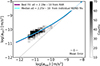 |
Fig. E.2. RAR of our intermediate-z sample, where abar and atot are derived from the RCs modelled in the MOND framework. The cross in the lower right corner indicates the mean 1σ uncertainties on the data points. The dotted black line shows the 1:1 relation. The purple curve represents the best-fit RAR, with |

The recovered a0|z ∼ 1 value is in fairly good agreement with the values of a0|z ∼ 1 obtained previously when the data were fitted with DM halos (Eq. 2, purple data point in Fig. 2), and is larger than the canonical z = 0 value (red star in Fig. 2). In Fig. E.2, we also plot as the cyan curve Eq.1 using for the characteristic acceleration scale the median value inferred for the sample from the individual MOND fits on the data cubes, i.e. a0|z ∼ 1 = 2.27 × 10⁻¹⁰ m/s2, which close to the a0|z ∼ 1 inferred from the fit to the RAR.
Following the procedure presented in Sect. 3.2, we also fit the RAR extracted from the MOND framework using the z-dependent acceleration scale (Eq. 1 substituting a0 with Eq. 3), and obtain
 (E.5)
(E.5)
To test whether this result is consistent with the values inferred from individual MOND fits, we also performed a direct linear regression of the best-fit a0 values from each galaxy as a function of z, which yields a slope  and an intercept
  , in fairly good agreement with the z-dependent fit to the RAR presented above (Eq. E.5), and with the values obtained in the main text (Eq. 4). Together, these results reinforce the presence of a systematic increase of the characteristic acceleration scale with redshift as we found previously when the data were fitted with DM halos (Sect. 3.2 and Appendix D).
We end this appendix by noting that these MOND fits underperform compared to the DM-based models (Appendix D) for over 60% of the sample using the Bayesian model comparison test as in Paper I.
Appendix F: Quantifying the z-evolution of the RAR
To complement the z-dependent RAR fit presented in Sect. 3.2, we show the full posterior distributions of all fitted parameters in Fig. F.1. The fit was performed on the whole sample using the MNR method implemented in Roxy (Bartlett & Desmond 2023), by replacing a0 in Eq. 1 with the redshift-dependent form defined in Eq. 3. In addition to the primary parameters, a0(0) and a1, the corner plot displays the intrinsic scatter of the relation, σintr, and the Gaussian hyperparameters μgauss and wgauss. Here, μgauss and wgauss represent the mean and standard deviation of the Gaussian prior on the true log(abar) values. The hyperparameters are also marginalised over when inferring a0(0) and a1. The 2D contours reveal no significant correlations, confirming that a0(0) and a1 are well constrained.
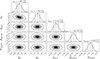 |
Fig. F.1. Corner plot showing the posterior distributions of the parameters from the redshift-dependent fit to the RAR for the full sample. The acceleration scale is replaced by a0(z) = a0(0)+a1 ⋅ z in the MOND-inspired interpolation function (Eq. 1). The Gaussian hyperparameters μgauss and wgauss define the mean and width of the Gaussian prior on the true log(abar) values, as implemented in Roxy, while σintr represents the intrinsic scatter of the RAR. The units of a0 and a1 are 10−10 m/s2, while for μgauss, wgauss, and σintr the units are in dex. The contours indicate the 68% and 95% confidence levels. |
This linear relation, using the best-fit values of a0(0) and a1 is shown as the purple line in Fig. 3. We note that this global fit is obtained from a single likelihood analysis of all individual data points and is not a regression through the a0 values obtained from the binned analysis, i.e. the black data points shown in Fig. 3. Because data points enter the fit with their full measurement uncertainties, higher-z measurements typically carry less statistical weight, and small offsets between the global relation and the binned estimates are therefore expected.
All Figures
|
Fig. 1. RAR for the MHUDF sample. The purple curve shows the best-fit RAR at 0.33 < z < 1.44 using Eq. (1), while the red and green curves show the McGaugh et al. (2016) relation at z = 0 and the Vărăşteanu et al. (2025) relation at z < 0.08, respectively. The black dotted line indicates the 1:1 relation. The histogram in the inset displays the residuals with respect to our fit. The cross in the upper left corner indicates the mean 1σ uncertainties. |
| In the text | |
|
Fig. 2. Best-fit a0 values obtained by fitting Eq. (1) on the full sample, using the resolved RAR tracks derived under different modelling assumptions. The purple data point shows a0|z ∼ 1 obtained using the DC14 halo profile applied uniformly to the full sample (Sect. 3.1). The cyan point shows a0|z ∼ 1 derived from a galaxy-by-galaxy best-fitting ΛCDM model, where each galaxy is assigned the DM profile that maximises its Bayesian evidence (Appendix D). The blue point shows a0|z ∼ 1 recovered from the MOND-based framework (Appendix E). The red star indicates the fiducial a0|z ∼ 0 from McGaugh et al. (2016), while the green star shows the result from Vărăşteanu et al. (2025). |
| In the text | |
|
Fig. 3. Redshift evolution of the characteristic acceleration scale. In each quantile-based z bin (blue bars), we fit the RAR with Eq. (1) to derive a0, with uncertainties shown as grey error bars. The star marks the SPARC z = 0 value. The purple line shows the predicted evolution, using the best-fitting parameters from the global z-dependent fit to the RAR for the full sample (i.e. using Eq. (1) where a0 was substituted with Eq. (3); see Eq. (4)). The red line shows the same, but including SPARC in the fit. The coloured shaded region shows the 1σ errors for the fits. |
| In the text | |
|
Fig. A.1. Stellar masses vs redshift for all MHUDF SFGs. The dashed black line indicates the mass completeness limit of the survey, which is reasonably complete for 0.2 < z < 1.5 down to log(M★/M⊙) = 8.6. The dashed red line shows the completeness of the parent sample from Paper I. The grey points show all SFGs observed in the MHUDF survey, the red-outlined points correspond to the galaxies analysed in Paper I, and the blue points indicate the galaxies studied in this work. The histograms on the top and right display the redshift and stellar-mass distributions, respectively, colour-coded to match the main panel. |
| In the text | |
|
Fig. B.1. Examples of the 3D disk-halo decomposition for the two galaxies from the sample. The solid black line represents the circular velocity vc(r) corrected for pressure support. The solid green curve represents the RC of the DM component. The solid orange and blue curves represent the disk and cold gas components, respectively. The light shaded regions show the 95% CI. The dotted brown line represents the stellar component measured using the multi-Gaussian expansion modelling of resolved stellar mass maps obtained from pixel-by-pixel SED fitting, while the dash-dotted green curve shows the DM component obtained independently from a 1D disk–halo decomposition. All velocities are intrinsic, i.e. corrected for inclination and instrumental effects, including seeing (PSF). The black dotted line shows the physical extent of a MUSE spaxel. |
| In the text | |
|
Fig. C.1. Left: Average mass-to-light ratios (M/L) in the K-band as a function of redshift for the MHUDF sample split into two M★ bins, the low-M★ bin (yellow) and high-M★ bin (orange), along with the evolution inferred for a sample of more than 5000 K-selected galaxies in Drory et al. (2004). The red star shows the M/L-K ratio adopted for the SPARC sample. Right: Impact of systematic disk mass offsets on the inferred a0(z). The black points correspond to the fiducial fits shown in Fig 3. The blue points show the inferred a0(z) assuming a global shift of +0.2 dex in the mass budget of the sample, while the green points show the same, but when assuming a global shift of +0.45 dex . The red star and dotted lines show the canonical a0(z = 0) inferred for the SPARC sample. |
| In the text | |
|
Fig. D.1. RAR of our intermediate-z sample, with abar and atot derived from the model RCs corresponding to each galaxy’s best-fitting ΛCDM halo profile. The coloured points indicate the halo profile used in the disk–halo decomposition. The cross in the lower right corner indicates the mean 1σ uncertainties on the data points. The dotted black line shows the 1:1 relation. The purple curve represents the best-fit RAR, with |
| In the text | |
|
Fig. E.1. Distribution of the MOND acceleration parameter a1. The purple histogram shows the recovered a1 values from individual galaxy fits. The vertical red line marks the reference value obtained from the RAR in the main text, |
| In the text | |
|
Fig. E.2. RAR of our intermediate-z sample, where abar and atot are derived from the RCs modelled in the MOND framework. The cross in the lower right corner indicates the mean 1σ uncertainties on the data points. The dotted black line shows the 1:1 relation. The purple curve represents the best-fit RAR, with |
| In the text | |
|
Fig. F.1. Corner plot showing the posterior distributions of the parameters from the redshift-dependent fit to the RAR for the full sample. The acceleration scale is replaced by a0(z) = a0(0)+a1 ⋅ z in the MOND-inspired interpolation function (Eq. 1). The Gaussian hyperparameters μgauss and wgauss define the mean and width of the Gaussian prior on the true log(abar) values, as implemented in Roxy, while σintr represents the intrinsic scatter of the RAR. The units of a0 and a1 are 10−10 m/s2, while for μgauss, wgauss, and σintr the units are in dex. The contours indicate the 68% and 95% confidence levels. |
| In the text | |
Current usage metrics show cumulative count of Article Views (full-text article views including HTML views, PDF and ePub downloads, according to the available data) and Abstracts Views on Vision4Press platform.
Data correspond to usage on the plateform after 2015. The current usage metrics is available 48-96 hours after online publication and is updated daily on week days.
Initial download of the metrics may take a while.