| Issue |
A&A
Volume 709, May 2026
|
|
|---|---|---|
| Article Number | A155 | |
| Number of page(s) | 15 | |
| Section | Cosmology (including clusters of galaxies) | |
| DOI | https://doi.org/10.1051/0004-6361/202558679 | |
| Published online | 13 May 2026 | |
Gas rotation and turbulence in the galaxy cluster Abell 2029
1
Dipartimento di Fisica e Astronomia “Augusto Righi” – Alma Mater Studiorum – Università di Bologna, Via Gobetti 93/2, 40129 Bologna, Italy
2
INAF, Osservatorio di Astrofisica e Scienza dello Spazio, Via Gobetti 93/3, 40129 Bologna, Italy
3
SRON Netherlands Institute for Space Research, Niels Bohrweg 4, 2333 CA, Leiden, The Netherlands
4
INFN, Sezione di Bologna, Viale Berti Pichat 6/2, 40127 Bologna, Italy
5
Department of Physics, University of Arkansas, 825 W Dickson st, Fayetteville, AR, USA
6
MIT Kavli Institute for Astrophysics and Space Research, 70 Vassar st., Cambridge, MA, USA
7
Department of Physics and Astronomy, The University of Alabama in Huntsville, Huntsville, AL 35899, USA
★ Corresponding author: This email address is being protected from spambots. You need JavaScript enabled to view it.
Received:
19
December
2025
Accepted:
19
March
2026
Abstract
Aims. We constrain the rotation and turbulent support of the intracluster medium (ICM) in Abell 2029 (A2029) using dynamical equilibrium models and a combination of state-of-the-art X-ray and microwave datasets.
Methods. The rotating turbulent ICM in the model has a composite polytropic distribution in equilibrium in a spherically symmetric, cosmologically motivated dark halo. The profile of rotation velocity and the distribution of turbulent velocity dispersion are described with flexible functional forms, which are consistent with the properties of synthetic clusters formed in cosmological simulations. Adopting realistic profiles for the metallicity distribution of the ICM and for the point spread function of XRISM and XMM-Newton, we tuned the observables of the intrinsic quantities of the plasma in our model via a Markov chain Monte Carlo algorithm to reproduce the radial profiles of the thermodynamic quantities as derived from the spectral analysis of the XMM-Newton and Planck maps and the measurements of the line-of-sight (LOS) nonthermal velocity dispersion and redshift (probing the LOS velocity) in the XRISM pointings.
Results. Our model accurately reproduces the measurements of redshift and LOS nonthermal velocity dispersion, and this was further demonstrated by simulating and analyzing synthetic counterparts of the XRISM spectra, in accordance with the posterior distributions we obtained. We measured the turbulence-to-total pressure ratio to be ≈2% across the 0–650 kpc radial range, and, under the hypothesis that rotation is the only bulk motion, we report a rotation-to-dispersion velocity ratio peaking at 0.15 between 200–600 kpc. The hydrostatic-to-total mass ratio is ≈0.97 at r2500, i.e., the radius enclosing an overdensity of 2500 times the average value. Further constraints on the presence and amount of rotation could be obtained through a full azimuthal coverage of A2029 with XRISM.
Key words: galaxies: clusters: general / galaxies: clusters: intracluster medium / galaxies: clusters: individual: Abell 2029 / X-rays: galaxies: clusters
© The Authors 2026
 Open Access article, published by EDP Sciences, under the terms of the Creative Commons Attribution License (https://creativecommons.org/licenses/by/4.0), which permits unrestricted use, distribution, and reproduction in any medium, provided the original work is properly cited.
This article is published in open access under the Subscribe to Open model. This email address is being protected from spambots. You need JavaScript enabled to view it. to support open access publication.
1. Introduction
Improving the accuracy in estimating the mass of galaxy clusters would reduce the systematics in the determination of the parameters that define the cosmological background (e.g., Pratt et al. 2019, for a review). Even though the matter content of galaxy clusters is dominated by dark matter, they are permeated by a hot, rarefied optically thin plasma known as the intracluster medium (ICM). The ICM manifests itself primarily in the X-ray band via both Bremsstrahlung and heavy-metal line emission (e.g., Sanders 2023, for a review), and in the microwave band, it manifests via weak distortions in the blackbody spectrum of the cosmic microwave background (CMB) caused by thermal and nonthermal motions of the ICM relative to the CMB rest frame (Sunyaev & Zeldovich 1972, 1980). A key step to improving the accuracy of dynamical mass estimates based on X-ray observations of the ICM is to go beyond the hydrostatic-equilibrium assumption (e.g., Pratt et al. 2019). However, the modest energy resolution of X-ray Charge Coupled Device (CCD) spectrometers, such as those aboard Chandra and XMM-Newton, and the limited sensitivity of microwave detectors have prevented characterization of the velocity field of the ICM, except for a small number of nearby clusters, whose measurements are nonetheless poor in precision (e.g., Sanders et al. 2020; Gatuzz et al. 2022b,a; Sanders 2023; Gatuzz et al. 2024). The launch of the XRISM satellite1 (Tashiro et al. 2018) following the short-lived Hitomi Soft X-ray Spectrometer marked the beginning of the era of high-resolution X-ray spectroscopy, which is capable of detecting shifts in the centroids and broadenings of the X-ray emission lines corresponding to ICM velocities down to ∼ 10 km s−1 in the inner regions of galaxy clusters. Thanks to the growing sample of clusters observed by Hitomi and XRISM (Hitomi Collaboration 2016; XRISM Collaboration 2025a,b,c) and the joint analysis of X-ray, Sunyaev-Zeldovich (SZ), and strong gravitational lensing data (Sayers et al. 2021; Chappuis et al. 2025), the low contribution of nonthermal motions to the ICM dynamics in their central regions is increasingly becoming solid evidence. However, the poor signal-to-noise ratio in the available data has so far limited these types of studies to a small sample of nearby massive clusters.
Some authors have attempted to address the specific question of whether and to what extent the ICM rotates. Bartalesi et al. (2025, hereafter B25), based on X-ray data of a sample of massive galaxy clusters, find that there is room for nonnegligible rotation in the ICM, with a typical peak rotation speed of ≈300 km s−1. Velocities of the ICM also imprint weak distortions in the CMB spectrum, known as the kinetic Sunyaev-Zeldovich (kSZ) effect, which can be observed in the microwave band, particularly with the upcoming Simons Observatory (Abitbol et al. 2025). The rotational component of kSZ has recently been detected at a 3.6σ confidence level through the analysis of the signal in the Planck images combined with the SDSS redshifts of the member galaxies in 25 nearby galaxy clusters (Goldstein & Hill 2025). The kinematics of the ICM has long been studied in clusters formed in cosmological hydrodynamical simulations, where rotation and turbulence play a minor yet relevant role in supporting the ICM against the cluster gravity. While the rotation of the ICM is expected to peak at intermediate radii (e.g., Baldi et al. 2017; Altamura et al. 2023), turbulence support is predicted to increase outward (e.g., Lau et al. 2013; Nelson et al. 2014; Angelinelli et al. 2020, hereafter A20). The XRISM spectra have the unprecedented potential to test these predictions, although they probe only spatially limited regions of nearby clusters. Significant azimuthal variations similar to those formed in cosmological simulations are expected in real systems (Nelson et al. 2014).
Abell 2029 (hereafter, A2029) is a massive nearby cluster at a redshift of z0 ≈ 0.0779, as inferred from the optical spectroscopy of the brightest cluster galaxy (BCG; XRISM Collaboration 2025b). The peak of the ICM emission lies close to its centroid (Eckert et al. 2022b), and no relative displacement nor motion between the BCG and ICM has been observed (XRISM Collaboration 2025b). The X-ray isophotes are well approximated by an elliptical shape that we estimate from the XMM-Newton soft images to have an emission-weighted average ellipticity of ≈0.08. Therefore, we can consider A2029 an exceptionally poorly disturbed cluster and, thus, a very close representation of a symmetric ICM in equilibrium within the potential well. It was one of the targets of XMM Cluster Outskirts Project (X-COP), a large observational campaign aimed at characterizing the profiles of the thermodynamic quantities of the ICM from the inner regions out to the outskirts by leveraging the joint analysis of the X-ray and SZ data (Eckert et al. 2017). For A2029, this campaign yielded a high-quality dataset of density, temperature, and thermal pressure profiles extending from the center to the outskirts (Ghirardini et al. 2019a, hereafter G19), which has been exploited by Ettori et al. (2019) and Eckert et al. (2022a) to derive hydrostatic-equilibrium models for A2029. More recently, during the verification phase of the XRISM mission, A2029 was observed with the microcalorimeter spectrometer XRISM/Resolve through three pointings along the northwest branch, with a total exposure of ≈500 ks. The spectra extracted from these three pointings revealed a low but still significant contribution from the nonthermal motions in the ICM, as compared to the temperatures measured from the same spectra (XRISM Collaboration 2025d, hereafter X25a). In this paper, we study the properties of A2029 as inferred by applying hydrodynamical-equilibrium models of the same family as those presented in B25, which include rotation and turbulence of the plasma, to data from the X-COP project and observed by XRISM/Resolve.
Given that XRISM is characterized by a large extent of the point spread function (PSF; ≈1.3 arcmin full width at half maximum), counts measured in the X-ray spectrum originate from photons emitted by the ICM in the plane-of-the-sky regions surrounding the pointing under analysis. If not properly accounted for, this effect, known as spatial-spectral mixing, introduces potentially significant contamination to the physical information encoded in the spectra. The most accurate, albeit computationally intensive, method to address this during the spectral forward-fitting involves adopting a thermal model with both spatial (in the plane of the sky) and spectral (in energy) dependence and stochastically simulating the paths of X-ray photons from the plane of the sky to the XRISM/Resolve focal plane. This technique, known as Monte Carlo spectral simulation, forward-folds the model through the instrument’s response characteristics. In the case of N adjacent pointings, it is standard to model the spectrum extracted from the j-th pointing as a combination of contributions from all i-th regions corresponding to the available pointings, where i, j = {1, …, N}. Assuming a Chandra broadband surface brightness map (treated as energy-independent), we ran Monte Carlo simulations to build a N × N matrix of specific ancillary response functions (ARFs), with the generic element ARFi, j. Multiplying the thermal emission model for the generic i-th region by ARFi, j yields an estimation of the fractional contribution of photons originating from the i-th region to the observed j-th spectrum. The N spectra were then simultaneously fit to infer the parameters of each i-th thermal model, primarily the shifts and broadening of the X-ray emission lines (e.g., Hitomi Collaboration 2018; XRISM Collaboration 2025a, and also X25a). Several factors may complicate or limit this approach: for example, the poor signal-to-noise ratio in the spectra extracted from the outer pointings, the small number of X-ray emission lines detected with high significance (in the outermost pointing of A2029 only three lines are detected at a 3σ confidence level in the energy range 2–10 keV; Sarkar et al. 2025), and the reduced contrast between the emission lines and the continuum in the presence of a ∼ 100 km s−1 line-of-sight (LOS) nonthermal velocity dispersion. The fluxes of the X-ray emission lines, necessary for the ICM velocity measurements, are determined by a combination of emission measure, temperature, and metallicity of each fluid element contributing to the observed spectrum. Thus, an accurate model-data comparison should simultaneously account for all of these effects.
Motivated by these issues, but limited by the huge computational cost of running a spectral simulation for every model evaluation in the fitting procedure, we adopted a two-step strategy. (i) In the Bayesian framework of model-data comparison, we tuned the average observable quantities of our model in the exposure regions to reproduce those inferred from the observational data from XMM, Planck, and XRISM/Resolve. (ii) From the optimized model, via a Monte Carlo spectral simulation we generated XRISM/Resolve-like observations of our A2029 model for the same pointings as for the real data. We then evaluated whether the synthetic XRISM/Resolve data reproduces the observed line shifts and broadenings as measured from the real data. For the sake of consistency with the mock observations, we redid the spectral reduction and analysis of the XRISM/Resolve data.
The paper is organized as follows. Sects. 2 and 3 detail the observational data and the model used for our analysis, respectively. The method and results of the joint fitting to X-COP and XRISM/Resolve data are presented in Sect. 4. In Sect. 5, we generate and compare synthetic spectra with the real ones. In Sect. 6 we summarize our work and the main results we obtained. In this work, we assume a flat Λ cold dark matter cosmological model with the present-day matter density parameter Ωm, 0 = 0.3 and Hubble constant H0 = 70 km s−1 Mpc−1. We define MΔ as the mass enclosed within a sphere of radius rΔ, where the average density is Δ times the average density of the Universe, ρcrit. We used the Heasoft package version 6.35, XSPEC software version 12.0, with the default atomic database AtomDB, and the calibration files of XRISM/Resolve from the CalDB v8 repository.
2. Observational data
This section outlines the observational datasets that we compare to our model in our analysis of A2029. Sect. 2.1 describes the reduction and analysis of the X-ray high-resolution spectra obtained with XRISM/Resolve. Sect. 2.2 details the measurements reported by G19 as part of the X-COP project and obtained from XMM-Newton observations at modest spectral resolution in the X-rays and from modeling of the SZ effect signal from Planck data.
2.1. Resolve data
During the verification phase of the XRISM mission, A2029 was observed by XRISM/Resolve with three (3 arcmin)×(3 arcmin) pointings (approximately, 270 kpc × 270 kpc at z0 = 0.0779) aligned along a contiguous arm in the northeast direction out to 668 kpc, which is close to r2500 ≈ 680 kpc (see Figure 1 of X25a). We refer to these pointings with an index m = {1, 2, 3}, where m = 1 indicates the central one and m= 3 the outermost one.
We began the data reduction process using the cleaned event files. We excluded events from pixel 12 (used for gain reconstruction) and pixel 27 (which exhibited unexpected scale jumps; see X25a, for details). We applied the standard screening procedure recommended in xapipeline and implemented in the Heasoft software. We extracted the high-resolution primary photon counts integrated over all remaining detector pixels, producing the spectral file for the m-th pointing. Using archival night Earth data and applying the same screening, we generated the non-X-ray background NXBm using rslnxbgen. Next, we built a new screened event file by excluding all the events of the m-th spectral file with PI values outside the 6000–20 000 range. From this file, we generated the redistribution matrix file (RMFm) using rslmkrmf2 and the ARFm of a point-like source being in the center of the XRISM/Resolve field of view (FoV) using xaarfgen. Given that the X-ray background is significantly lower than the thermal emission in all the observations, as evidenced in Fig. 2 of X25a, we neglected it in our analysis. As discussed in Sect. 2 of X25a, for the m-th pointing the systematic uncertainties on the position of the emitting lines in the (6–7) keV range and their broadening is measured to be equal to or lower than ±0.15 eV and ±6 km s−1, respectively.
We began the spectral analysis for the generic m-th pointing with its corresponding reduced spectrum. Using the grppha task of Heasoft, we binned it to ensure at least one count per bin in each bin3. In XSPEC we subtracted from each of them the corresponding non-X-ray background with the command backgrnd. We accounted for the galactic absorption with the model tbabs (Wilms et al. 2000), fixing the column density, NH, to 3 × 1020 cm−2 as recommended by X25a. We then fit the m-th spectrum in the energy range 3 − 10 keV with the thermal emission model for a uniform and homogeneous plasma in collisional-ionization equilibrium (CIE), bapec4 (Smith et al. 2001). Given that no significant parameter correlations are expected as shown by the spectral simulations of Bartalesi et al. (2024) (hereafter, B24, see their Sect. 5.2), we estimated their 1σ errors as those obtained from the diagonal terms of the covariance matrix, using the Levenberg-Marquardt algorithm as implemented in XSPEC. Table 1 reports the measurements of the redshift, zu, m, and LOS nonthermal velocity dispersion, σv, m, for the three pointings (m = 1, 2, 3), which we compared to the model in Sect. 4. The velocity of the uniform and homogeneous plasma with respect to z0 in the m-th pointing, um (positive for receding ICM), and the barycentric velocity of the Earth, vbaryc, m, determine zu, m, according to (e.g., Roncarelli et al. 2018)
 (1)
(1)
Measurements from the XRISM/Resolve spectra.
Here, c is the light speed and vobs, m = vbaryc, m + um, with vbaryc, m = 26 km s−1 for m = {1, 2} and vbaryc, 3 = −27 km s−1. As discussed in Sect. 2 of X25a (see their Table 3), the plasma in the m = {2, 3} spectra is significantly blueshifted with respect to z0 (see also the differences between zu, m and z0 in Table 1 for m = {2, 3}). When we compared our model with the Resolve data, we therefore assumed approaching (i.e., negative) rotation velocities of the plasma.
2.2. Data from XMM and Planck observations
We now present the SZ data and X-ray spectral results for A2029 obtained from the spectral analysis of G19. These data are available on the X-COP website5.
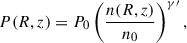
A2029 was observed with XMM-Newton through multiple pointings forming a mosaic. Assuming the cluster center to coincide with the peak of the X-ray surface brightness map, the mosaic covers a symmetric region around the cluster center, extending out to a projected radial distance of approximately 1488 kpc. G19 extracted 14 X-ray spectra, each from a circular annulus indexed with i, with inner and outer radii  and
and  , respectively (see Sect. 2.4 G19, for details). Each spectrum was fit using the apec emission model (a version of bapec without LOS nonthermal velocity broadening; see Sect. 2.1; Smith et al. 2001), yielding measurements of the normalization of the thermal continuum, Normi, the temperature, Ti, and the metallicity, Zi, of an uniform and homogeneous plasma in CIE. G19 also computed the brightness
![Mathematical equation: $$ \begin{aligned} \mathcal{N} _{i}= \frac{Norm_{i}}{\pi \left[ \left(\hat{R}_{i + 1}/ [\mathrm {arcmin}] \right)^2 - \left(\hat{R}_{i}/ [\mathrm {arcmin}] \right)^2 \right]}\cdot \end{aligned} $$](/articles/aa/full_html/2026/05/aa58679-25/aa58679-25-eq4.gif) (2)
(2)
The measurements of 𝒩i and Ti taken from the X-COP website are compared to our model in Sect. 46.
The Planck observation of A2029 results in a SZ signal map that resembles a square box in the plane of the sky, centered at the center of A2029 and with a side length of 7 Mpc. G19 modeled the SZ signal map, under the assumption that the thermal SZ effect dominates the signal (i.e., the relation between the “SZ pressure” and the Compton-parameter in Eq. (3) of G19 holds). Assuming spherical symmetry of the ICM distribution and adopting a realistic profile for the azimuthally averaged Planck PSF, they performed a geometric deprojection of the SZ signal, obtaining measurements of the “SZ pressure” in ten concentric spherical shells (see Sect. 2.5 of G19, for details). Given that, as discussed in detail in G19, the innermost three shells have radial widths smaller than the full width at half maximum of the Planck PSF, we exclude them from our analysis. In the X-COP website, a covariant matrix accounts for the statistical errors and the cross-correlations between the values of PSZ, j at all j. Given that the diagonal terms of the covariance matrix dominate, we include only these diagonal terms in the error budget of these measurements. In Sect. 4, we compare our model to the measurements of the thermal “SZ pressure”, PSZ, j, in seven spherical shells, indexed by j = {1, …, 7} and ranging from ≈800 kpc out to 3.5 Mpc.
3. Model of pressure-supported rotating ICM
Sections 3.1 and 3.2 detail, respectively, the intrinsic and observable properties of the axisymmetric cluster model with turbulent and rotating plasma used in our analysis. The turbulence is assumed to be isotropic and the rotation is such that the surfaces of constant angular velocity are cylinders.
3.1. Intrinsic properties of the model
We adopt a cylindrical reference frame (R, ϕ, z), with the origin at the minimum of the gravitational potential Φ. As in B25, the self-gravity of the plasma is neglected. Φ(r), with  the spherical radius, is a spherically symmetric Navarro-Frenk-White (NFW; Navarro et al. 1996) potential, fully specified by the virial mass M200 and concentration c200. The rotation curve of the plasma is (e.g., Bianconi et al. 2013; B25)
 (3)
(3)
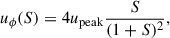
where S = R/Rpeak, upeak and Rpeak are the peak rotation speed and its radius, respectively. Baldi et al. (2017) showed that this functional form reproduces the average rotation speed profile of the ICM in clusters formed in a cosmological simulation. The full expression for the effective potential Φeff(R, z) in our model is provided in Equations (24) and (25) of B24.
The plasma number density and the total (thermal plus turbulent) pressure of a polytropic distribution in equilibrium in the axisymmetric potential Φeff are (e.g., Tassoul 1978)
![Mathematical equation: $$ \begin{aligned} n(R, z) = n_0 \left\{ 1 - \frac{\gamma \prime - 1}{\gamma \prime } \frac{\rho _0}{P_0} \left[\Phi _{\rm {eff}}(R, z) - \Phi _{\rm {eff,0}}\right] \right\} ^{\frac{1}{\gamma \prime - 1}} \end{aligned} $$](/articles/aa/full_html/2026/05/aa58679-25/aa58679-25-eq7.gif) (4)
(4)
and
 (5)
(5)
respectively, where Φeff,0 = Φeff(R0, 0), n0 = n(R0, 0), P0 = P(R0, 0), γ′ is the polytropic exponent and R0 is a generic radius in the equatorial plane. Here, ρ0 = ρ(R0, 0), where ρ = nμmp is the gas mass density. mp is the proton mass and μ = 0.6 the mean molecular weight, assuming a metallicity of 0.3 times the solar value throughout the cluster.
We considered a composite polytropic distribution with three distinct polytropic exponents:  ,
,  , and
, and  , such that
  . The transitions occur at radii RCEN (from
  to
to  ) and R★ (from
  to
to  ) in the equatorial plane. In Eqs. (4) and (5), the reference potentials for the transitions in the meridional plane are Φeff,0 = {Φeff,CEN, Φeff,★} for R0 = {RCEN,R★}, respectively, where Φeff,CEN = Φeff(RCEN, 0) and Φeff,★ = Φeff(R★, 0). The corresponding reference plasma properties are n0 = n★ and P0 = P★ for R0 = R★, and n0 = n(RCEN, 0) and P0 = P(RCEN, 0) for R0 = RCEN. Accordingly, γ′ takes the value of
  ,
,  or
or  for Φeff(R, z) <Φeff,CEN, Φeff,CEN ≤ Φeff(R, z) < Φeff,★ and Φeff(R, z) ≥ Φeff,★, respectively. The two-exponent composite-polytropic distribution of B24 and B25 is recovered in the limit case
  .
.
As in B25, the turbulent pressure is  , where Tgas is the plasma temperature and kB the Boltzmann constant. The distribution of the turbulent-pressure-to-total-pressure ratio follows
![Mathematical equation: $$ \begin{aligned} \alpha _{\rm {turb}}(P) = (\alpha _{\rm {inf}}- \alpha _0) \frac{\ln \left[1 + P / (\xi P_\star ) \right]}{P / (\xi P_\star )} + \alpha _0. \end{aligned} $$](/articles/aa/full_html/2026/05/aa58679-25/aa58679-25-eq22.gif) (6)
(6)
where α0 and αinf are, respectively, the asymptotic values for P → ∞ and P → 0, and ξ defines the transition between α0 and αinf. This expression can provide a good representation of the median profile of the turbulent support of the ICM in clusters formed in the cosmological simulation analyzed by Angelinelli et al. (2020) (see Sect. 3.1 of B25).
We define the parameter  as the equivalent temperature associated with the total pressure support at the reference point (R★, 0) in the meridional plane. This model has 14 parameters:
  ,
,  ,
,  , R★, RCEN, n★, T★, M200, c200, upeak, Rpeak, ξ, αinf, and α0.
3.2. From the intrinsic to the observable quantities of the model
We adopted a Cartesian reference system (x, y, z), with the origin located at the minimum of Φ. In our model, this point coincides with the point with the highest value of the plasma density. We fixed the redshift of the point with the highest plasma density in our model to z0. We assumed that our axisymmetric model is observed with the symmetry and rotation axis z in the plane of the sky, i.e. in the configuration that maximizes the component of the rotation speed of the plasma along the LOS. The x-axis is chosen to lie along the LOS. The y-axis in the plane of the sky is oriented along the NE–SW direction of A2029 (see Fig. 1 of X25a), i.e. along the direction sampled with the Resolve pointings, with positive values in the NE sector. For the sake of simplicity, we approximate the FoV of Resolve as a square with the two perpendicular sides of length 3 arcmin, parallel to either the y-axis or the z-axis, and with centers in the plane-of-the-sky points (0, 0), (3 arcmin, 0) and (6 arcmin, 0) for m = {1, 2, 3}, respectively. In this simplified configuration, only the m = 0 pointing is symmetric with respect to the rotation axis z.
We considered a generic quantity Q(R, z) dependent only on the intrinsic quantities in the model, as described in Sect. 3.1. We then introduced the polar coordinates in the y-z plane  and
and  . In our analysis, we used only quantities evaluated at z = 0. The integral of Q(R, 0) along the LOS is
 (7)
(7)
where  . Hereafter, unless stated otherwise, we report the projected quantities of the model approximated as circularly symmetric, with profiles
  .
.
In Appendix A.1, we describe how we convolved  with a circularly symmetric PSF profile to obtain
  when we approximated the evaluation of the PSF profile at z = 0 and
  in the general case. When
  is weighted over a realistic circularly symmetric projected metallicity profile of A2029, as detailed in Appendix A.2, we obtain
  .
.
We now consider the i-th circular annulus in the plane of the sky, with inner and outer radii  and
and  , respectively. The integral of the quantity
  , with w = {0, K, A}, in the i-th circular annulus is (see Eq. (D.3) of B25)
![Mathematical equation: $$ \begin{aligned} I_{i,w}[Q] = 2\pi \int _{\hat{R}_{i}}^{\hat{R}_{i + 1}} \hat{R}\mathrm{d} \hat{R}Q_{w}(\hat{R}), \end{aligned} $$](/articles/aa/full_html/2026/05/aa58679-25/aa58679-25-eq40.gif) (8)
(8)
where QLOS, QK and QA are defined above.
Now, we consider in the plane of the sky the m-th rectangle with a side of length yup, m − ylow, m parallel to y-axis and the other of length zup, m = 1.5 arcmin (for all m) parallel to the z-axis. For m = {1, 2, 3}, we define ylow, m = {0, 1.5, 4.5} arcmin and yup, m = {1.5, 4.5, 7.5} arcmin, respectively (at z0, 1 arcmin ≈88 kpc). The integral of QZ (see Appendix A.2) in the m-th rectangle is
![Mathematical equation: $$ \begin{aligned} S_{m}[Q] = \int _{0}^{z_{\mathrm{up},m}} \mathrm{d} z \int _{y_{\mathrm{low},m}}^{y_{\mathrm{up},m}} \mathrm{d} y Q_{\mathrm{Z} }\left(\sqrt{y^2 + z^2}\right). \end{aligned} $$](/articles/aa/full_html/2026/05/aa58679-25/aa58679-25-eq41.gif) (9)
(9)
The analog of the normalization of the thermal continuum measured from our model in the i-th circular annulus in the plane of the sky, with inner and outer radii  and
and  , respectively, is
![Mathematical equation: $$ \begin{aligned} Norm_{i,w}= C I_{i,w}\left[n_{\rm {H}}n_{\rm {e}}\right], \end{aligned} $$](/articles/aa/full_html/2026/05/aa58679-25/aa58679-25-eq44.gif) (10)
(10)
where nH and ne are the hydrogen-equivalent and electron number densities of the plasma. Given that metallicity gradients have a negligible impact on the plasma distribution in equilibrium in the gravitational potential, we simplify the model by assuming a constant metallicity of 0.3 times the solar value. This implies nH = 1.17ne and ne = n/1.94, with n obtained from Eq. (4). In our model, we assume n(R, z) = 0 for x, y, z > rSZ, where RSZ is the outer radius of the outermost spherical shell in which the SZ data have been extracted. ![Mathematical equation: $ C= 10^{-14} / \left [ 4\pi {D_{\rm{ang}}}^2 (1+z_0)^2 \right] $](/articles/aa/full_html/2026/05/aa58679-25/aa58679-25-eq45.gif) , with Dang the angular distance of the cluster, is the normalization factor adopted in XSPEC. As accurate approximation to the spectroscopically measured temperature in the presence of a nonneglible temperature gradient in the ICM, Mazzotta et al. (2004) proposed the spectroscopic-like temperature, which is measured from our model in the i-th circular annulus in the plane of the sky as
, with Dang the angular distance of the cluster, is the normalization factor adopted in XSPEC. As accurate approximation to the spectroscopically measured temperature in the presence of a nonneglible temperature gradient in the ICM, Mazzotta et al. (2004) proposed the spectroscopic-like temperature, which is measured from our model in the i-th circular annulus in the plane of the sky as
![Mathematical equation: $$ \begin{aligned} T_{i,w}=\frac{I_{i,w}\left[n_{\rm {H}}n_{\rm {e}}T_{\rm {gas}}^{3/4}\right]}{I_{i,w}\left[n_{\rm {H}}n_{\rm {e}}T_{\rm {gas}}^{-1/4}\right]}, \end{aligned} $$](/articles/aa/full_html/2026/05/aa58679-25/aa58679-25-eq46.gif) (11)
(11)
where Tgas is obtained as described in Sect. 3.1. In a set of high-resolution X-ray spectral simulations for a cluster formed in a cosmological simulation, Roncarelli et al. (2018) found the emission-weighted LOS velocity and velocity dispersion as accurate approximations of the corresponding measurements inferred with the bapec model.
We now consider the velocity vector of the plasma in our axisymmetric model, defined at a generic point (x, y, z) as  , where ux = uϕ(R)cos ϕ, uy = uϕ(R)sinϕ and uϕ is the rotation speed of the plasma in Eq. (3).
  and
and  are the unit vectors defining the x and y directions. In our configuration for the model (see above), the LOS component of u corresponds to ux, which for y ≥ 0 is equal to uϕRl/R, where
  for w = {0, A}, respectively. The emission-weighted LOS rotation speed measured from our model in the i-th circular annulus is
![Mathematical equation: $$ \begin{aligned} u_{i,w}= \frac{I_{i,w}[n_{\rm {H}}n_{\rm {e}}u_\phi R_{l}/ R]}{I_{i,w}[n_{\rm {H}}n_{\rm {e}}]}\cdot \end{aligned} $$](/articles/aa/full_html/2026/05/aa58679-25/aa58679-25-eq51.gif) (12)
(12)
When measured from our model in the m-th rectangle in the plane of the sky, the emission-weighted LOS rotation speed is
![Mathematical equation: $$ \begin{aligned} u_{\mathrm{ew},m}= \frac{S_{m}[n_{\rm {H}}n_{\rm {e}}u_\phi \bar{R}/ R]}{S_{m}[n_{\rm {H}}n_{\rm {e}}]}\cdot \end{aligned} $$](/articles/aa/full_html/2026/05/aa58679-25/aa58679-25-eq52.gif) (13)
(13)
In addition to the thermal velocity dispersion accounted for in the bapec emission model, the contributions at any (x, y, z) in our axisymmetric model to the LOS velocity dispersion evaluated at (y, z) come from the 1D turbulent velocity dispersion,  and the spread in ux(R, ϕ) along the x-axis. The emission-weighted nonthermal LOS velocity dispersions of the plasma as measured from our model in the i-th circular annulus and in the m-th rectangle in the plane of the sky are
![Mathematical equation: $$ \begin{aligned} \sigma _{\mathrm{v},i}= \frac{I_{i,0}\left[n_{\rm {H}}n_{\rm {e}}\sqrt{\sigma _{\rm {turb,1D}}^2 + \left(u_\phi \hat{R}/ R - u_{i,0} \right)^2} \right]}{I_{i,0}\left[n_{\rm {H}}n_{\rm {e}}\right]} \end{aligned} $$](/articles/aa/full_html/2026/05/aa58679-25/aa58679-25-eq54.gif) (14)
(14)
and
![Mathematical equation: $$ \begin{aligned} \sigma _{\mathrm{v,ew},m}= \frac{S_{m}\left[n_{\rm {H}}n_{\rm {e}}\sqrt{\sigma _{\rm {turb,1D}}^2 + \left(u_\phi \bar{R}/ R - u_{i,0}\right)^2} \right]}{S_{m}[n_{\rm {H}}n_{\rm {e}}]}, \end{aligned} $$](/articles/aa/full_html/2026/05/aa58679-25/aa58679-25-eq55.gif) (15)
(15)
respectively.
The PSZ, j in the j-th spherical shell, with inner and outer radii rj and rj + 1, respectively, is evaluated in our model following Sect. 3.2 of B25:
 (16)
(16)
where η is a dimensionless parameter accounting for the possible systematic offset between the electron pressure of the ICM and that measured from the Compton y-parameter maps.
4. Joint fitting of X-ray data from XMM and Resolve and of SZ data from Planck
Our model, presented in Sect. 3, is tuned to reproduce via a Markov chain Monte Carlo (MCMC) algorithm the measurements of the normalization of the thermal continuum, spectroscopic temperature, SZ pressure, redshift, and LOS nonthermal velocity dispersion obtained from XMM, Planck and XRISM data (see Sect. 2). Sect. 4.1 describes the statistical method, while Sect. 4.2 presents the results.
4.1. Statistical method
Assuming K(d) for XMM in Eq. (A.2) (see Appendix A.1) and using Eqs. (10), (11) and (16), we evaluate Normi, K, Ti = Ti, K and PSZ, j of the plasma in the model in the i-th circular annulus in the plane of the sky and j-th spherical shell, respectively (we recall that the normalization of the PSZ, j profile is regulated by η, defined in Sect. 3.2). Using Eq. (2) with Normi = Normi, K, we then compute 𝒩i from our model in the i-th circular annulus. Given the axial symmetry of the model, we limit the evaluation of σv, m and zu, m to y ≥ 0. Assuming K(d) for XRISM in Eq. (A.5) and using Eqs. (13) and (15), we evaluate uew, m and σv,ew, m from the model in the m-th rectangular region, respectively. Given that the m = 1 integration region in the y-z plane is symmetric with respect to the z-axis (which in our model is assumed to be the rotation axis), the rotation manifests itself as a contribution to the LOS velocity dispersion. This implies zu, 1 = z0 and  . In the m = {2, 3} pointings, which are not symmetric with respect to the z-axis, the rotation of the plasma in our model manifests itself as a shifting of the X-ray emission lines measured via the redshift zu, m that we obtain from Eq. (1) with um = −uew, m. In these cases, σv, m = σv,ew, m.
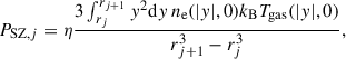
The statistical errors, σstat, on the observed 𝒩i, Ti and PSZ, j are obtained as the average between the upper and lower 1σ errors reported in the X-COP website. The statistical errors on the observed zu, m and σv, m are taken from Table 1. Following B25, we introduce three parameters, ϵN, ϵT, and ϵSZ, to account for a systematic contribution, ϵσstat, with ϵ = {ϵN,ϵT,ϵSZ}, to the uncertainty in the measurements of 𝒩i, Ti and PSZ, j7, respectively. ϵN, ϵT and ϵSZ are assumed to have the same values in all the radial bins. We denote each datum, whether 𝒩i, Ti, PSZ, j, zu, m and σv, m, with Dq, b where q = {1, 2, 3, 4, 5}, respectively, and b indicates the spatial bin corresponding to this datum. We assumed the generic Dq, b to have a normal distribution with median equal to the corresponding value computed from the model and standard deviation  for q = {1, 2, 3} and σstat for q = {4, 5}. It follows that the generic likelihood of the datum Dq, b,
  , is a normal distribution with the same median and standard deviation as described above.
The 18 free parameters in the MCMC sampling are  ,
,  , ν★ ≡ log(n★/[10−3cm−3]), Tequiv,★, R★, M200, lnc200, upeak, Rpeak, log ξ, αinf, α0, η, log ϵN, log ϵT and log ϵSZ (see Sect. 3.1, for the definition of the model parameters). We assume uniform prior distributions on all these parameters within the ranges listed in Table 2. We briefly comment on the lower bound of the prior on the radius Rpeak where the rotation curve peaks. There is a growing consensus that turbulence is the main driver of the re-acceleration of relativistic electrons, which manifests observationally in A2029 as a radio mini-halo, an extended synchrotron emission detected at low radio frequencies and in the inner regions (Govoni et al. 2009; Murgia et al. 2009). Based on this interpretation, we expect a significant turbulent contribution to the observed σv, 1, although also the rotation can contribute to σv, 1 (see above). We realize this scenario in our model by conservatively setting the lower bound of the uniform prior on Rpeak approximately to the radial extent of the first Resolve pointing (≈150 kpc). The MCMC algorithm maximizes the logarithmic posterior distribution of the generic parameter vector
  :
: ![Mathematical equation: $ \ln \mathcal P ({\boldsymbol \theta}) = \sum_{q = 1}^{5} \sum_{b} \ln \left[\mathcal L \left({D_{q,b}}\right)\right] $](/articles/aa/full_html/2026/05/aa58679-25/aa58679-25-eq63.gif) , if all the values θ1, …, θ18 are within the corresponding prior ranges, and
, if all the values θ1, …, θ18 are within the corresponding prior ranges, and  , otherwise.
Lower and upper bounds of the uniform prior distributions of the MCMC parameters and their marginal posterior credible interval.
4.2. Results from the posterior distribution of our model
When the MCMC algorithm converges to a stationary posterior8, we draw the posterior sampling that we use for our analysis. The relative frequency of the values of the parameters in the posterior sampling can be visualized in the corner plot presented in Appendix C. The credible interval obtained from the marginal posterior sampling of each parameter is reported in Table 2. For the analysis of the results of the MCMC run, from the posterior sampling we randomly extract 100 parameter vectors that we consider as a representative set of the posterior distribution of our model.
Following Sect. 5 of B25, we evaluated the accuracy of our model in reproducing the observational measurements through the residual, defined at each spatial radial bin as the difference between the observational measurement and the corresponding model value, normalized to the latter. The comparison of the values computed from the model for this representative set of the posterior sampling with those obtained by modeling the signal from X-ray and microwave observations is presented in Fig. 1. The values of 𝒩i, Ti and PSZ, j in our model reproduce well the corresponding values for all the values of i and j, with median residuals of ≈0.005, 0.001 and 0.007, respectively. However, we note that, in the radial range (300–700) kpc, corresponding to i = {7, …, 11}, the values of 𝒩i and Ti between the median model and the observational constraints differ by a factor up to 3.2 times the total (statistical plus systematic) uncertainty, probably due to local fluctuations either in the density or temperature profiles, whereas the pressure profile, obtained by deprojecting and combining gas density and temperature, is well modeled within 1σ uncertainty. In Sect. 3.1 we introduced a three-zone polytropic distribution, with parameters  and RCEN (the transition radius from the central regions, with polytropic index
  , to those intermediate with
  ) in addition to those used by B24 and B259 (see their Sect. 3). The MCMC run constrains the marginal posterior distribution of RCEN to a well limited radial range, approximately corresponding to ≈100 kpc (≈0.05 r200) from the center, and the marginal posterior distribution of
  to values more than 10σ discrepant from the median
  (see Table 2). This implies that the density and temperature measurements in the core of A2029 require two polytropic components transitioning at a radius of ≈0.05 r200. We note that, consistently with our results, Ghirardini et al. (2019b) find polytropic index increasing with increasing radius not only for A2029, but also for the other three cool-core clusters in their X-COP sample. The parameter η (see Sect. 3.2) inferred in our model, 0.96 ± 0.1, is consistent within 1σ credible interval with the median of the η distribution for the other X-COP clusters, inferred by B25 (see their Appendix A). In addition, the consistency of η with unity, which is the expected value for a spherically symmetric ICM distribution, implies that current data support the absence of offset between the X-ray and SZ-derived thermal pressure profiles (e.g., Kozmanyan et al. 2019). The median values of ϵN, ϵT and ϵSZ inferred from our model are 0.40, 0.13 and 0.06, respectively (see the corner plot in Appendix C). These values indicate that the contribution of the systematic errors to the total error budget is subdominant with respect to the statistical uncertainties. The median inferred value of ϵN is larger than those of ϵT and ϵSZ but consistent with the lower end of the distribution of the corresponding parameter reported in Sect. 5.1 of B25. In all the rectangular pointings, the values of zu, m and σv, m from the intrinsic properties of our model are consistent with the observed ones, with median residuals of 0.001. In Sect. 5, generating and analyzing synthetic counterparts of all the XRISM/Resolve observed spectra for the ICM in our model, we derive mock measurements of zu, m and σv, m that are compared with those inferred here.
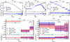 |
Fig. 1. Profiles (upper part of each panel) and residuals (lower part of each panel) of the brightness ( |


From the posterior sampling, we computed a few relevant quantities for the interpretation of the results. At a given point in the equatorial plane, we evaluate the rotation velocity, uϕ(R), through Eq. (3), σturb,1D}(R, 0) (defined in Sect. 3.2) and the 1D velocity dispersion of the plasma, ![Mathematical equation: $ {\sigma_{\rm{gas,1D}}}(R, 0) = \sqrt{P(R, 0) / \left[{\upmu}{\mathrm{m}_{\mathrm{p}}} n(R, 0)\right]} $](/articles/aa/full_html/2026/05/aa58679-25/aa58679-25-eq75.gif) , where P(R, 0) and n(R, 0) are obtained as described in Sect. 3.1. As a measure of the dynamical importance of rotation, we computed, as a function of radius R, the ratio between uϕ(R) and σgas,1D(R, 0) in the equatorial plane, uϕ/σgas,1D. We compute the turbulent-pressure-to-total-pressure ratio αturb, defined by Eq. (6), to quantify the dynamical importance of the turbulence.
, where P(R, 0) and n(R, 0) are obtained as described in Sect. 3.1. As a measure of the dynamical importance of rotation, we computed, as a function of radius R, the ratio between uϕ(R) and σgas,1D(R, 0) in the equatorial plane, uϕ/σgas,1D. We compute the turbulent-pressure-to-total-pressure ratio αturb, defined by Eq. (6), to quantify the dynamical importance of the turbulence.
Figure 2 shows uϕ, uϕ/σgas,1D, σturb,1D, and αturb for the representative set of the posterior sampling mentioned above as a function of the cylindrical radius R. We limit ourselves to R in the range (0–668) kpc, corresponding to the range along the positive y-direction sampled by the three XRISM/Resolve pointings. Both σturb,1D and αturb exhibit nearly radial constant profiles, with median values of 100 km s−1 and 0.02, respectively. Instead, the median profiles of both uϕ and uϕ/σgas,1D increase outward, reaching a median peak of 200 km s−1 and of 0.15 at R between 200 and 600 kpc. The broad 16th–84th percentile interval for Rpeak, spanning (250–540) kpc (see Fig. C.1), indicates that the current XRISM/Resolve data put weak constraints on the position of the uϕ peak. In Fig. 2, we also plot the profiles representative of the average properties of clusters formed in cosmological N-body hydrodynamical simulations. In particular, we take the average uϕ profile of a maximally rotating sample selected within the MUSIC-2 sample10 and the median αturb profile of the Itasca sample from B17 and A2011, respectively. Similarly to our uϕ, profile, the B17 profile increases outward, but their median peak of uϕ≈ 400 km s−1 in the plotted range is inconsistent to a 1σ credible interval with our inference. Instead, although the shape of our αturb profile seems not too different from that of A20, the latter slightly increases outward and is inconsistent to a 1σ credible interval with our inferred values.
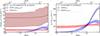 |
Fig. 2. Left panel: radial profiles of squared rotation-velocity-to-velocity-dispersion ratio and turbulent-to-total pressure ratio for A2029. Right panel: radial profiles of turbulent velocity dispersion and rotation velocity for A2029. We overplot the median and average profiles of turbulence (left panel) and rotation velocity (right panel) measured in simulated clusters by A20 and B17 (dark red and dark blue regions; see text, for details), respectively. The dashed lines indicate the median profiles; the shaded regions represent the 16th–84th percentile interval profiles. The A20 and B17 profiles are obtained as in Figs. 2 of B25 and 3 of B24, respectively. The 16th–84th percentile interval of B17 profile refers to the uncertainty in the posterior distribution of our model parameters. |
In X25a, the same spectral data of XRISM/Resolve used in this work are analyzed, and an effective nonthermal velocity dispersion (obtained by adding in quadrature the measured velocity dispersion and the bulk motion) is combined with the thermal component to construct a total pressure in equilibrium in an NFW potential. Our αturb is consistent within 1.5σ credible interval with the corresponding median value of the nonthermal-to-total pressure ratio (see their Fig. 6). However, our median profile does not support the outward-decreasing trend they report. The improvements in the underlying physical model and in the accuracy of the modeling of the PSF effect (see Sect. A.1), as demonstrated by the comparison with the results of the spectral simulations in Sect. 5, may explain why our model has a flatter profile than that inferred by X25a.
For the Monte Carlo spectral simulations run in Sect. 5.1, we use the “extflat” mode in the software HeaSim that assumes circular symmetry of the distribution of the quantities of our model in the plane of the sky. Given that the characteristic of the rotation is a dipole-like pattern in the map of the projected LOS rotation velocity, with positive values on one side of the cluster and negative on the opposite side, this assumption appears to be less justified for the rotation observables. This dipole-like pattern can be approximately modeled by considering Eqs. (A.8) and (A.9) instead of Eqs. (13) and (15) in the derivation of zu, m and σv, m in the analysis above. Using Eqs. (A.8) and (A.9) and assuming the same prior as in Table 2, we refit our model to the same observational measurements via a MCMC sampling. We find that the rotation and turbulence profiles, obtained from the latter inference, are similar to those of Fig. 2.
5. Comparison with the results of the spectral simulations
The Heasim software, part of the standard HEASoft package, is an event generator specifically developed for Monte Carlo spectral simulations with high-energy focusing telescopes, including XRISM. For a pointing on the sky, it produces a synthetic event file that records the photons generated according to an input X-ray emissivity and registered through an XRISM/Resolve-like instrument, making it an ideal tool for forward-folding the diffuse X-ray emission associated with our dynamical model for A2029. For the representative set of the posterior sampling extracted in Sect. 4.2, we want to produce synthetic counterparts of all three XRISM/Resolve spectra under consideration and to measure the shifts and broadenings of their emission lines. Section 5.1 details the procedure used to generate and analyze synthetic counterparts of all the XRISM/Resolve event files for the three pointings (see Sect. 2.1) for the generic parameter vector θ of our model. Sect. 5.2 presents and discusses the results of the analysis of the synthetic spectra for values of θ belonging to the representative set of the posterior distribution.
5.1. Setup of the spectral simulations
Assuming that the position of the minimum of the gravitational potential of our model coincides with the sky coordinates of the m = 1 pointing center, we define a circular region extending out to 11.2 arcmin (≈950 kpc at z0) from the center in the plane of the sky. This region is divided into 90 circularly symmetric, concentric annuli, linearly spaced in radius. Consistent with Sect. 3, the i-th annulus has inner and outer radii  and
and  , respectively. At any given pointing m and annulus i, fixing NH to the same value as in Sect. 2.1, we compute in XSPEC the emission model tbabs×bapecm, i, with the parameters Normi, Ti, Zi, zu, m, i and σv, m, i defined for a given θ as follows. Note that the quantities without the subscript m do not depend on the characteristics of each pointing. We take Normi = Normi, 0 and Ti = Ti, 0, where Normi, 0 and Ti, 0 are obtained from Eqs. (10) and (11), respectively. Zi is evaluated at the radius
  according to Eq. (A.4). We derive ui, 0 and σv, i from Eqs. (12) and (14), respectively. We recall that the rotation manifests itself as a contribution to σv, m and zu, m in the m = 1 and m = {2, 3} pointings, respectively (see Sect. 4.1, for details). For m = 1 and a given i, um = 0 in Eq. (1) and
  . It is important to note that in this Section the value of um in Eq. (1) depends on both the pointing m and the annulus i. For m = {2, 3} and a given i, um = −ui, 0 in Eq. (1), and σv, m, i = σv, i.
As standard in the framework for forward-folding the emission from an extended source through the instrumental responses, the vignetting12 and PSF models are treated separately from the ARF. We take the ARFm of a point-like source being in the center of the Resolve FoV for the m-th pointing from Sect. 2.1. It already accounts for the photon loss of a point-like source due to PSF scattering outside the detector. Also HeaSim simulates this effect in a manner appropriate for the extended emission model we provide (see below). If we were to use the standard ARFm for the HeaSim simulations, we would model twice the PSF photon scattering. To avoid this, we use for the HeaSim simulations a corrected ARF of a point-like source, defined as ARFfc, m = ARFm/0.804, where 0.804 is the fraction of the PSF model, for a centered point-like source, lying inside the detector region13. For the m-th mock observation, Heasim uses RMFm, ARFfc, m and NXBm14 (see Sect. 2.1), the energy-dependent PSF and vignetting files from the Cycle 1 calibration files15. The sky coordinates are fixed to the RA and DEC values recorded in the corresponding m-th event file. To have similar relative error on the inferred values of the redshift in the three pointings, we rescale the exposure time to be set in the HeaSim spectral simulation for a given mock observation by the emissivity.
For the m-th pointing and the i-th annulus, we generate a photon distribution in position and in energy,  , via a Monte Carlo sampling, using the “extflat” mode of HeaSim that considers the emission model tbabs × bapecm, i to be uniformly distributed over all the i-th plane-of-the-sky annulus and to vanish elsewhere. Then, the ray-tracing simulations, run with Heasim, redistribute the photon distribution
 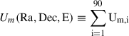 in position in the focal plane of the detector and in energy according to the Resolve characteristics. The simulation results in an event file for each value of m containing the counts that a Resolve-like instrument would measure from the polytropic distribution of turbulent and rotating ICM defined by θ.
Considering all the counts reported in the m-th synthetic event file except for those detected in pixel 12, we extract the m-th spectrum. Following the same procedure as for the real m-th spectrum (see Sect. 2.1, for details), we bin and, then, fit the m-th mock spectrum to infer zu, m and σv, m of a uniform and homogeneous plasma in CIE. We repeat the procedure described above for each pointing for each selected θ.
5.2. Results of the spectral simulations
In addition to the metallicity, the density and temperature of the ICM, which mainly shape the spectral continuum in the X-rays, regulate the fluxes of the emission lines, whose shifts and broadenings encode the spectral signatures of rotation and turbulence that we want to constrain with XRISM/Resolve data in Sect. 4.2. For a given θ, as the model provides a distribution of the density and temperature, which was constrained in Sect. 4.2 to reproduce the XMM measurements, the model provides, via the generation of the photon distribution  , precise predictions on the count rate as a function of the spectral energy in the m-th XRISM/Resolve pointing. In line with the statistical approach adopted for our study, in this Section we compare the median count rate within the m-th synthetic spectra of a representative set of the posterior distribution with the corresponding observed value in each energy bin. Though our approach in principle allows reconstruction of the emission observed in the three XRISM/Resolve pointings according to the XMM observations, the detailed investigation of the match between the XMM and XRISM/Resolve observations lies beyond the scope of this work.
In addition to Um, the combination of RMFm, ARFfc, m, NXBm and the model for the PSF (see Sect. 5.1, for details) determines the count rate in the m-th mock spectrum. Now, we report the systematics in these components of the spectral simulation that can introduce offsets between the m-th count rates observed by XRISM/Resolve and inferred using the posterior of our model. The requirement for the precision of in-flight calibration of the XRISM/Resolve effective area is ±10%, both over a broad energy range, as well as within several narrower energy bins (of a few keVs size) (see Miller et al. 2021). This work is ongoing, and current discrepancies between XMM and XRISM Resolve and Xtend can be up to ±20%, as reported by XRISM Collaboration (2025e), leading to offsets between the XRISM/Resolve and XMM count rates ranging from 0.8 to 1.2. We recall that HeaSim assumes a PSF model that reproduces the on-ground azimuthally averaged measurements for the Soft X-ray Imager of the mission Hitomi. Given that the PSF distribution is expected to scatter out of the central pointing a significant fraction of the photons originating from the central regions of a cool-core cluster with a very peaked density profile, such as A2029, the PSF uncertainties16 can also realistically produce an offset in the range (0.9–1.1) for m = 1 and (0.95–1.05) for m = {2, 3}.
For the sake of simplicity, in Sect. 5.1, we assumed the X-ray emission to be circularly symmetric in the plane of the sky. Under this assumption, the ratio between the total observed and mock count rates in the (3–10) keV energy range, Rcount, m, is17 1.18 ± 0.01, 1.17 ± 0.02 and 1.09 ± 0.02 for m = {1, 2, 3}, respectively. Note that the quoted errors are only statistical, while as argued above, systematic uncertainties at the level of 20–30% dominate the error budget, but are hard to quantify at this time. However, the XMM mosaic map analyzed by G19 shows enhanced emission in the NE azimuthal sector, the region covered by all XRISM/Resolve pointings. For each pointing, we adopt a correction factor, Raz, m, defined in Appendix B as the ratio between the count rate in the NE sector and the azimuthally averaged value, independently of the spectral energy. After multiplying the mock count rate in each energy bin by Raz, m, the corrected Rcount, m becomes 1.04 ± 0.02 and 0.93 ± 0.02 for m = 2 and m = 3, respectively. For the central pointing (m = 1), the azimuthal variations in the X-ray emission are unlikely to produce an offset in Rcount, 1 as substantial as for m = {2, 3}. In conclusion, the corrected Rcount, m is consistent with unity, i.e. no offset between predicted and observed count rates, within the combined systematic (due to PSF model and effective area measurements) and statistical uncertainties for any m.
Figure 3 presents for each pointing the comparison between the mock and observed count rates in spectral energy bins in the (3–10) keV (the total count rates are reported in the legend). We find no statistical evidence for either a trend of the ratio between observed and mock count rates with the spectral energy or an offset in energy bins of a few keV. The best-fit metallicity measured in each mock spectrum is consistent within a 2σ confidence interval with the corresponding observed value.
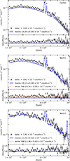 |
Fig. 3. Count rates (upper part of each panel) and residuals (lower part of each panel) of the m = {1, 2, 3} (top, middle and bottom panels, respectively) XRISM/Resolve pointings of A2029 as a function of the spectral energy. The median count rate of the mock spectrum and its 16th–84th percentile interval are represented by the dashed blue line and blue shaded region, respectively. The observational data are the black dots, whereas the black vertical error bars indicate the 1σ uncertainties and the horizontal error bars the bin extent. The value of Raz, m for m = {2, 3} (see text) is indicated by the horizontal dotted red line in the residual panels. |
Now that we have established that the density, temperature and metallicity distributions of the plasma in our model are consistent with the X-ray emission resolved by XRISM/Resolve in the three spectra, we compare the line shifts and broadenings between the m-th synthetic and observed spectrum. The values of zu, m and σv, m, obtained by fitting the emission model for a uniform and homogeneous plasma in CIE to the m-th spectral data, quantify the average shift and broadening of the X-ray emission lines in the m-th spectrum. The middle panels of Fig. 1 show that the mock measurements of zu, m and σv, m reproduce the corresponding XRISM/Resolve values, with median residuals of 0.001, respectively, which are consistent with those reported in Sect. 4.2. This comparison demonstrates that the profiles of turbulence and rotation shown in Fig. 2 remain accurate in reproducing the observed values of zu, m and σv, m in the m-th XRISM/Resolve spectrum even when we use the more accurate, but computationally more expensive procedure carried out in this Section.
6. Summary and conclusions
We have presented an axisymmetric equilibrium model that reproduces the observed properties of the ICM in the galaxy cluster A2029. Building on the formalism used by B24 and B25, the model describes a composite-polytropic distribution of a rotating and turbulent plasma in equilibrium in the gravitational potential of a spherically symmetric NFW dark matter halo. The profile of rotation velocity and the distribution of the turbulent velocity dispersion are described with relatively flexible functional forms that are consistent with the corresponding average radial profiles derived from the analyses of the MUSIC-2 and Itasca samples of clusters formed in cosmological simulations by B17 and A20, respectively (see Sect. 3.1).
We reduced and conducted spectral analysis of the data from the three XRISM/Resolve pointings for A2029, which were acquired during the performance verification phase of the mission and sampled its northeast direction out to r2500 ≈ 669 kpc. In addition to the measurements of the LOS nonthermal velocity dispersion (σv) and redshift (zu, probing the LOS component of the ICM velocity) in the three XRISM spectra, we considered the measurements of the normalization of the thermal continuum (which scales with the gas density squared) of the spectroscopic plasma temperature and of the SZ-derived thermal pressure as obtained by G19 in the radial bins defined in the XMM-Newton and Planck maps (see Sect. 2).
When performing the comparison with observational data, we assumed that our model is observed edge-on, in particular with the rotation and symmetry axis orthogonal to the NE direction, and we fixed the systemic redshift of our model to that of BCG (z0). We fit the radial metallicity profile of Mernier et al. (2017) to the XMM measurements of G19 and assumed the best-fit profile throughout our entire analysis. In the derivation of zu and σv from the model, we weighted the kinematic observables over this metallicity distribution in the plane of the sky, and assuming realistic circularly symmetric profiles for the PSFs of XRISM and XMM, we convolved the observable quantities of our model with them. Under these assumptions, from the intrinsic properties of the plasma in our model, we computed the observable quantities that approximate those recovered from the spectral analysis (see Sect. 3.2). Via an MCMC sampling, we fit this model simultaneously to all the aforementioned observational measurements to infer the posterior distribution of the model parameters (see Sect. 4).
According to the posterior distribution of our model, under the same assumptions of metallicity and PSF profiles, we generated an ensemble of synthetic spectral counterparts for the three XRISM/Resolve pointings of our model. After showing that the synthetic spectrum of each pointing is consistent (within the systematic uncertainties) with the corresponding observed spectrum, we conducted the spectral analysis of the mock data as for the observed ones (see Sect. 5).
The main results of our work are the following.
-
Our model accurately reproduces the observational measurements of zu and σv in the three pointings for A2029, as further demonstrated by comparing the measurements of zu and σv from synthetic and observed XRISM/Resolve spectra (see Sect. 5.2).
-
The inferred turbulent-to-total pressure ratio has a flat profile across all the radial range (0–650 kpc), with a median value of ≈0.02, and the inferred rotation-velocity-to-velocity-dispersion ratio peaks at a distance on the NE direction from the center in the range 250–650 kpc, with a median value of 0.15 (see Sect. 4.2).
-
Following Sect. 4.3 of B24, we evaluated the ratio between the hydrostatic mass and the true mass of our halo model, which at R = r2500 ≈ 669 kpc is 0.97 ± 0.01.
Some of the assumptions underlying our analysis, such as rotation as the only bulk motion contributing to the LOS velocity observed in the off-center XRISM pointings and the position angle of the rotation axis, will soon be tested with an approved XRISM/Resolve pointing toward the eastern region of A202918. Further constraints on the presence and amount of rotation could be obtained through a full azimuthal coverage of A2029 with XRISM.
The orientation of the rotation axis in the three-dimensional space is difficult to constrain observationally. In our analysis, we arbitrarily assumed that the rotation axis is orthogonal to the LOS. This choice of the LOS is convenient not only because it simplifies the computation of the observables (see Eqs. (10)–(16)), but also because it allowed us (under the assumption of rotation as the only bulk motion) to put a lower limit on the intrinsic rotation speed for a given LOS velocity. For any other LOS, the inferred intrinsic rotation speed would tend to be higher. An extreme case would be that of an LOS parallel to the rotation axis with no rotation-induced line centroid shift regardless of the intrinsic rotation speed.
X25c find that clusters observed by XRISM/Resolve in regions not strongly affected by AGN feedback – namely, those outside the central few hundred kiloparsecs in cool-core systems or throughout non-cool-core clusters – typically exhibit turbulent-to-total pressure ratios lower than the medians of their counterparts formed in three cosmological simulations (TNG-Cluster, GADGET-X, and GIZMO-Simba). Nevertheless, these measured ratios generally remain within the 68% scatter of simulated values, except for the two outer pointings of A2029. In those cases, the median turbulent-to-total pressure ratios, which are below 0.01 (see Fig. 5 of X25c), have a probability of less than 1% of occurring within the simulated cluster population (see their Section 4.2 for discussion). Our inferred rotation and turbulence profiles for the ICM in A2029 lie significantly below those originally derived by B17 and A20 (see Sect. 4.2 and Fig. 2). Consequently, our complementary analysis supports the X25c finding that the turbulent support in observed clusters tends to fall below that measured in these simulations. However, our flat profile of the turbulent-to-total velocity dispersion ratio, with a median value above 0.01, reduces the tension between A2029 and its simulated analogs in the outer pointings reported by X25c. Our turbulent-to-total pressure ratio places A2029 at the lower end of the simulated cluster distribution, consistent with the behavior of all other objects observed in regions not strongly influenced by AGN feedback. The accurate forward-modeling of the PSF scattering effect in deriving the model quantities analogous to the measurements may explain differences from the results of X25a, which were adopted by X25c. These discrepancies further highlight the importance of employing more sophisticated model–data comparison methods, such as those presented in this work, potentially including Monte Carlo spectral simulations.
Using optical data, Castellani et al. (2025) investigated the possible rotation of the galactic component in A2029. They detected a statistically significant dipole-like pattern in the redshift distribution of the member galaxies, from a few tens of kiloparsecs from the center out to beyond r500: the galaxies tend to be approaching in the northern regions and receding in the southern regions. Interpreting this pattern as the rotation of the system of member galaxies, they derived a rotation axis along the NW–SE direction, which is broadly consistent with what is assumed in our analysis. The measured peak rotation velocity and rotation-velocity-to-velocity-dispersion ratio, 220 km s−1 and 0.18, respectively, agree within the 1σ credible interval with our inferred values. The formation history of A2029 likely determines the relationship between the rotational properties of its main baryonic components. For example, Roettiger & Flores (2000) predict a rotating plasma and a static galactic component in an off-axis post-merger cluster. If future XRISM/Resolve observations confirm our results, they would indicate a remarkable agreement between the rotational properties of the galactic and plasma components of A2029 and offer valuable constraints on its formation scenario.
The validity of hydrostatic mass estimates of galaxy clusters at ∼ Megaparsec radii, crucial for cosmological parameter inference, could be robustly assessed through spatially resolved high-resolution X-ray spectroscopy of cluster outskirts. Such measurements are expected to be feasible with future missions such as ESA’s NewAthena (Cruise et al. 2025) and the Chinese mission HUBS (Bregman et al. 2023).
Acknowledgments
We thank the referee for the constructive comments that helped improve the paper. T.B. thanks the financial support from the European Union NextGenerationEU. S.E. thanks the financial contribution from Theory Grant/Bando INAF per la Ricerca Fondamentale 2024 on “Constraining the nonthermal pressure in galaxy clusters with high-resolution X-ray spectroscopy” (1.05.24.05.10). This work extensively used the Python packages Numpy (Harris et al. 2020), Scipy (Virtanen et al. 2020), Matplotlib (Hunter 2007), emcee (Foreman-Mackey et al. 2013), Cython (Behnel et al. 2011) and Astropy (Price-Whelan et al. 2018) and the HEaSArch softwares Xspec and HeaSim.
References
- Abitbol, M., Abril-Cabezas, I., Adachi, S., et al. 2025, JCAP, 2025, 034 [Google Scholar]
- Altamura, E., Kay, S. T., Chluba, J., & Towler, I. 2023, MNRAS, 524, 2262 [NASA ADS] [CrossRef] [Google Scholar]
- Angelinelli, M., Vazza, F., Giocoli, C., et al. 2020, MNRAS, 495, 864 [NASA ADS] [CrossRef] [Google Scholar]
- Baldi, A. S., De Petris, M., Sembolini, F., et al. 2017, MNRAS, 465, 2584 [NASA ADS] [CrossRef] [Google Scholar]
- Bartalesi, T., Ettori, S., & Nipoti, C. 2024, A&A, 682, A31 [NASA ADS] [CrossRef] [EDP Sciences] [Google Scholar]
- Bartalesi, T., Ettori, S., & Nipoti, C. 2025, A&A, 697, A17 [NASA ADS] [CrossRef] [EDP Sciences] [Google Scholar]
- Behnel, S., Bradshaw, R., Citro, C., et al. 2011, Comput. Sci. Eng., 13, 31 [Google Scholar]
- Bianconi, M., Ettori, S., & Nipoti, C. 2013, MNRAS, 434, 1565 [NASA ADS] [CrossRef] [Google Scholar]
- Bregman, J., Cen, R., Chen, Y., et al. 2023, Sci. China: Phys. Mech. Astron., 66, 299513 [NASA ADS] [CrossRef] [Google Scholar]
- Castellani, D., Ferrami, G., Grillo, C., & Bertin, G. 2025, A&A, 701, A250 [NASA ADS] [CrossRef] [EDP Sciences] [Google Scholar]
- Chappuis, L., Eckert, D., Sereno, M., et al. 2025, A&A, 699, A141 [NASA ADS] [CrossRef] [EDP Sciences] [Google Scholar]
- Croston, J. H., Arnaud, M., Pointecouteau, E., & Pratt, G. W. 2006, A&A, 459, 1007 [NASA ADS] [CrossRef] [EDP Sciences] [Google Scholar]
- Cruise, M., Guainazzi, M., Aird, J., et al. 2025, Nat. Astron., 9, 36 [Google Scholar]
- Eckert, D., Ettori, S., Pointecouteau, E., et al. 2017, Astron. Nachr., 338, 293 [Google Scholar]
- Eckert, D., Ettori, S., Pointecouteau, E., van der Burg, R. F. J., & Loubser, S. I. 2022a, A&A, 662, A123 [NASA ADS] [CrossRef] [EDP Sciences] [Google Scholar]
- Eckert, D., Ettori, S., Robertson, A., et al. 2022b, A&A, 666, A41 [NASA ADS] [CrossRef] [EDP Sciences] [Google Scholar]
- Ettori, S., Ghirardini, V., Eckert, D., et al. 2019, A&A, 621, A39 [NASA ADS] [CrossRef] [EDP Sciences] [Google Scholar]
- Foreman-Mackey, D., Hogg, D. W., Lang, D., & Goodman, J. 2013, PASP, 125, 306 [Google Scholar]
- Gatuzz, E., Sanders, J. S., Canning, R., et al. 2022a, MNRAS, 513, 1932 [NASA ADS] [CrossRef] [Google Scholar]
- Gatuzz, E., Sanders, J. S., Dennerl, K., et al. 2022b, MNRAS, 511, 4511 [NASA ADS] [CrossRef] [Google Scholar]
- Gatuzz, E., Sanders, J., Liu, A., et al. 2024, A&A, 692, A108 [NASA ADS] [CrossRef] [EDP Sciences] [Google Scholar]
- Ghirardini, V., Eckert, D., Ettori, S., et al. 2019a, ApJ, 621, A41 [Google Scholar]
- Ghirardini, V., Ettori, S., Eckert, D., & Molendi, S. 2019b, A&A, 627, A19 [NASA ADS] [CrossRef] [EDP Sciences] [Google Scholar]
- Goldstein, S., & Hill, J. C. 2025, ArXiv e-prints [arXiv:2512.10951] [Google Scholar]
- Govoni, F., Murgia, M., Markevitch, M., et al. 2009, A&A, 499, 371 [NASA ADS] [CrossRef] [EDP Sciences] [Google Scholar]
- Harris, C. R., Millman, K. J., van der Walt, S. J., et al. 2020, Nature, 585, 357 [NASA ADS] [CrossRef] [Google Scholar]
- Hitomi Collaboration (Aharonian, F., et al.) 2016, Nature, 535, 117 [Google Scholar]
- Hitomi Collaboration (Aharonian, F., et al.) 2018, PASJ, 70, 9 [NASA ADS] [Google Scholar]
- Hunter, J. D. 2007, Comput. Sci. Eng., 9, 90 [NASA ADS] [CrossRef] [Google Scholar]
- Kaastra, J. S. 2017, A&A, 605, A51 [NASA ADS] [CrossRef] [EDP Sciences] [Google Scholar]
- Kozmanyan, A., Bourdin, H., Mazzotta, P., Rasia, E., & Sereno, M. 2019, A&A, 621, A34 [NASA ADS] [CrossRef] [EDP Sciences] [Google Scholar]
- Lau, E. T., Nagai, D., & Nelson, K. 2013, ApJ, 777, 151 [NASA ADS] [CrossRef] [Google Scholar]
- Mazzotta, P., Rasia, E., Moscardini, L., & Tormen, G. 2004, MNRAS, 354, 10 [NASA ADS] [CrossRef] [Google Scholar]
- Mernier, F., de Plaa, J., Kaastra, J. S., et al. 2017, A&A, 603, A80 [NASA ADS] [CrossRef] [EDP Sciences] [Google Scholar]
- Miller, E. D., Sawada, M., Guainazzi, M., et al. 2021, SPIE Conf. Ser., 11444, 1144426 [Google Scholar]
- Murgia, M., Govoni, F., Markevitch, M., et al. 2009, A&A, 499, 679 [NASA ADS] [CrossRef] [EDP Sciences] [Google Scholar]
- Navarro, J. F., Frenk, C. S., & White, S. D. M. 1996, ApJ, 462, 563 [Google Scholar]
- Nelson, K., Lau, E. T., Nagai, D., Rudd, D. H., & Yu, L. 2014, ApJ, 782, 107 [NASA ADS] [CrossRef] [Google Scholar]
- Pratt, G. W., Arnaud, M., Biviano, A., et al. 2019, SSR, 215, 25 [NASA ADS] [Google Scholar]
- Price-Whelan, A. M., Sipőcz, B. M., Günther, H. M., et al. 2018, AJ, 156, 123 [NASA ADS] [CrossRef] [Google Scholar]
- Read, A. M., Rosen, S. R., Saxton, R. D., & Ramirez, J. 2011, A&A, 534, A34 [NASA ADS] [CrossRef] [EDP Sciences] [Google Scholar]
- Roettiger, K., & Flores, R. 2000, ApJ, 538, 92 [Google Scholar]
- Roncarelli, M., Gaspari, M., Ettori, S., et al. 2018, ApJ, 618, A39 [Google Scholar]
- Sanders, J. S. 2023, ArXiv e-prints [arXiv:2301.12791] [Google Scholar]
- Sanders, J. S., Dennerl, K., Russell, H. R., et al. 2020, A&A, 633, A42 [EDP Sciences] [Google Scholar]
- Sarkar, A., Miller, E., Ota, N., et al. 2025, PASJ, 77, S254 [Google Scholar]
- Sayers, J., Sereno, M., Ettori, S., et al. 2021, MNRAS, 505, 4338 [NASA ADS] [CrossRef] [Google Scholar]
- Sembolini, F., Yepes, G., De Petris, M., et al. 2013, MNRAS, 429, 323 [NASA ADS] [CrossRef] [Google Scholar]
- Smith, R. K., Brickhouse, N. S., Liedahl, D. A., & Raymond, J. C. 2001, ApJ, 556, L91 [Google Scholar]
- Štofanová, L., Simionescu, A., & Kaastra, J. S. 2025, A&A, 694, A149 [NASA ADS] [CrossRef] [EDP Sciences] [Google Scholar]
- Sunyaev, R. A., & Zeldovich, Y. B. 1972, Comm. Astrophys. Space Phys., 4, 173 [Google Scholar]
- Sunyaev, R. A., & Zeldovich, Y. B. 1980, MNRAS, 190, 413 [NASA ADS] [CrossRef] [Google Scholar]
- Tashiro, M., Maejima, H., Toda, K., et al. 2018, SPIE Conf. Ser., 10699, 1069922 [Google Scholar]
- Tassoul, J.-L. 1978, Theory of Rotating Stars [Google Scholar]
- Vazza, F., Jones, T. W., Brüggen, M., et al. 2017, MNRAS, 464, 210 [Google Scholar]
- Virtanen, P., Gommers, R., Oliphant, T. E., et al. 2020, Nat. Methods, 17, 261 [Google Scholar]
- Wilms, J., Allen, A., & McCray, R. 2000, ApJ, 542, 914 [Google Scholar]
- XRISM Collaboration (Audard, M., et al.) 2025a, Nature, 638, 365 [Google Scholar]
- XRISM Collaboration (Audard, M., et al.) 2025b, ApJ, 982, L5 [Google Scholar]
- XRISM Collaboration (Audard, M., et al.) 2025c, ApJ, 985, L20 [Google Scholar]
- XRISM Collaboration (Audard, M., et al.) 2025d, PASJ, 77, S242 [Google Scholar]
- XRISM Collaboration (Audard, M., et al.) 2025e, A&A, 702, A147 [Google Scholar]
- XRISM Collaboration (Audard, M., et al.) 2025f, ApJ, 993, L11 [Google Scholar]
The procedure we follow to generate RMFm is detailed at the link https://heasarc.gsfc.nasa.gov/docs/xrism/analysis/ttwof/index.html
Given that X25a binned the reduced spectrum using the optimal binning algorithm of Kaastra (2017) as implemented in the ftgrouppha task of the Heasoft package, we verified that the difference in the inferred values of zu, m and σv, m (see below) between these two binnings does not exceed the corresponding 1σ statistical error.
The spectral analyses of XMM-Newton and XRISM/Resolve data provide independent constraints on the normalization of the thermal continuum (proportional to the density squared) and the temperature of the ICM in the inner regions of A2029. However, given that both quantities may be subject to uncertainties in the cross-calibration of the telescope effective areas, the instrumental PSF and in the NXB modeling, in the comparison with our model, we adopt only the XMM-Newton measurements, which additionally offer more complete azimuthal coverage of the cluster in the plane of the sky (see text). Sect. 5.2 discusses in part the consistency of the properties of the plasma in our model, which reproduces the XMM spectral results, with the XRISM/Resolve spectral data.
These nuisance parameters cover a wide range of possible systematics, related both to intrinsic source properties and instrument calibration. These include, for instance, the presence of unresolved clumps in the XMM maps as well as uncertainties in the PSFs of XMM and Planck.
Using the same sampler as in B25 (see their Appendix B, for details), we run the MCMC algorithm for 10 000 iterations with 500 chains. Empirically, we find that the posterior becomes stationary after 3000 iterations, but we conservatively assume that the iteration 5000 is the endpoint of the burn-in phase. The posterior sampling is obtained by selecting all the  for all the chains every 700 iterations, starting from the endpoint of the burn-in phase.
The parameter Rbreak of B24 and B25 was renamed as R★ in this work.
The MUSIC-2 sample (Sembolini et al. 2013) is composed by 258 clusters with M200 > 7 × 10¹⁴ M⊙ re-simulated with a zoom-in technique in a cosmological environment. B17 classified as rotating clusters those with a spin parameter (see their Eq. (2), for its definition) larger than 0.07, which are the 4% of the Sembolini et al. (2013) population. We present the average properties of this rotating population in the radiative run, which refers to the simulation including radiative cooling and subgrid models for feedback from active galactic nuclei and from massive stars. However, as discussed in B17, the average rotational properties of these systems are similar to those of the rotating population in the non-radiative run.
The Itasca (Vazza et al. 2017) sample is composed by nine clusters with 0.5 < M100/(1014 M⊙) < 4 that were re-simulated with a higher resolution in the cosmological environment. Taking snapshots of these clusters at redshift 0 < z < 2, separated by at least one dynamical time of the cluster, they built a sample of 68 clusters and showed that its mass function closely resembles that predicted at z= 0.
The vignetting is the decrease in the measured count rate switching from on-axis to off-axis observations of a point-like source.
This value is reported in the xaarfgen log output when run for every m (see Sect. 2.1).
We recall that this background file has been built while excluding the pixel 27 that, instead, in the simulation is included.
For sake of completeness, we report that, based on a comparison of pixel-to-pixel relative count rates and with the corresponding predictions of ray-tracing simulations, X25a conservatively quantified that the uncertainties in the XRISM/Resolve PSF can introduce an offset within the range 0.7–1.3 (see their Sect. 3.2).
The relative error on Rcount, m is estimated by adding in quadrature the relative uncertainties of broadband mock and observed count rates. We note that the statistical uncertainty of the count rate of each synthetic spectrum has two contributions: the Poisson noise introduced in the spectral simulation and the uncertainty in the parameter values in the posterior.
As described in Sect. 3.2, we assume a rotation axis in the plane of the sky orthogonal to the A2029 arm sampled with performance verification phase pointings and aligned with this forthcoming pointing. In the latter, our model predicts an LOS velocity close to zero and an LOS nonthermal velocity dispersion similar to or higher than in the m = 2 spectrum.
For a reference model, we tested values of dmax increased by 1.1 for both XMM and XRISM PSF profiles, finding insignificant differences from the profiles of Fig. 1.
These PSF data represent azimuthally averaged values taken from the on-ground measurements for the Soft X-ray Imager on board of Hitomi mission, the twin predecessor of the XTEND imager on board the XRISM mission. Given the similarity in the instrumentation design of XRISM/XTEND and XRISM/Resolve, their PSFs are expected to be nearly identical.
r500 ≈ 1488 kpc is the value obtained using ![Mathematical equation: $ {r_{500}}= \left[3 M_{500} / (2000\pi G {\rho_{\rm{crit}}}) \right]^{1/3} $](/articles/aa/full_html/2026/05/aa58679-25/aa58679-25-eq84.gif) from the median hydrostatic M500 reported in Table 1 of Ettori et al. (2019).
from the median hydrostatic M500 reported in Table 1 of Ettori et al. (2019).
Appendix A: Convolution with the instrumental point spread function and weighting over the metallicity
A.1. Point spread function convolution of the observable quantities
To emulate the effect of photon scattering caused by the telescope PSF on the observable quantities derived from spectral analysis, we convolve the spatial distributions of the corresponding quantities of our model in the plane of the sky with a circularly symmetric PSF profile.
To this purpose, we define the function
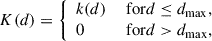 (A.1)
(A.1)
where k(d) is the PSF profile, dmax a truncation radius and d the distance between two points in the plane of the sky. When convolved with K,  becomes
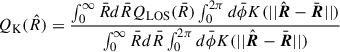 (A.2)
(A.2)
where  and
and  are two distinct position vectors in the y-z plane.
To reduce the computational cost, it can be convenient to limit the evaluation of  to z = 0 and approximate Eq. (A.2) as
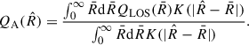 (A.3)
(A.3)
We fix dmax to 1.15 arcmin and 5.75 arcmin for XMM and XRISM, respectively19. We assume for XMM ![Mathematical equation: $ k(d) = 1/[1 + (d / {R_{\rm{c}}})^2]^\alpha $](/articles/aa/full_html/2026/05/aa58679-25/aa58679-25-eq92.gif) , where Rc = 0.145 arcmin (≈ 12.8 kpc at z0) and α = 1.68, as best-fit King-profile values to the Read et al. (2011) PSF measurements obtained by combining the three XMM-Newton cameras with weight of 0.25 for MOS and 0.5 for pn as in Croston et al. (2006). For XRISM/Resolve, we construct k by interpolating with a cubic spline the PSF measurements reported in the HeaSim support files20. Given that in the comparison with the model we take only the measurements of zu and σv from the results of the XRISM/Resolve spectral analysis (see Sect. 4.1), we use the PSF data only for 8 keV photons, the energy closest to the Fe-K complex (6 – 7) keV, which dominates the spectral features used to derive those measurements.
, where Rc = 0.145 arcmin (≈ 12.8 kpc at z0) and α = 1.68, as best-fit King-profile values to the Read et al. (2011) PSF measurements obtained by combining the three XMM-Newton cameras with weight of 0.25 for MOS and 0.5 for pn as in Croston et al. (2006). For XRISM/Resolve, we construct k by interpolating with a cubic spline the PSF measurements reported in the HeaSim support files20. Given that in the comparison with the model we take only the measurements of zu and σv from the results of the XRISM/Resolve spectral analysis (see Sect. 4.1), we use the PSF data only for 8 keV photons, the energy closest to the Fe-K complex (6 – 7) keV, which dominates the spectral features used to derive those measurements.
A.2. Metallicity profile
We assume that the projected distribution of the metals of A2029 in the plane of the sky is circularly symmetric, with profile (Mernier et al. 2017; Štofanová et al. 2025)
![Mathematical equation: $$ \begin{aligned} Z(\hat{R}) = \frac{A}{[1 + \hat{R}/ (r_{500} B)]^C} \left\{ 1-D\exp \left[-\frac{\hat{R}}{r_{500} F} \left(1+\frac{\hat{R}}{r_{500} E}\right) \right] \right\} + G, \end{aligned} $$](/articles/aa/full_html/2026/05/aa58679-25/aa58679-25-eq93.gif) (A.4)
(A.4)
where r500 = 1448 kpc21, and A, B, C, D, E, F and G are free parameters. We evaluate eq. (A.4) at the radius  for the generic i-th circular annulus, with inner and outer radii
  and
and  . Maximizing a Gaussian log-likelihood, we fit it to the G19 measurements. Fig. A.1 shows the inferred profile, with best-fit parameters A = 1.34, B = 5.15 × 10⁻³, C = 4.81 × 10⁻¹, D = 4.14 × 10⁻¹, E = 1.69 × 10⁻¹, F = 2.10 × 10⁻² and G = 9.68 × 10⁻², compared with the G19 measurements. Throughout this work, we assume that the metallicity distribution in the plane of the sky follows eq. (A.4) with these best-fit parameter values.
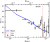 |
Fig. A.1. Model metallicity (blue line) as a function of the projected radius |

When weighted over  and convolved with K(d) via eq. (A.3) (see sect. A.1, for details),
  becomes
 (A.5)
(A.5)
A.3. 1D convolution of rotational properties
The 1D convolution of the generic projected quantity QLOS (defined in Eq. (7)), weighted over the projected metallicity profile Z (taken from Eq. (A.5)), is
 (A.6)
(A.6)
where K is defined in Eq. (A.1). The 1D integration in the segment of length equal to the extent of the FoV of XRISM/Resolve for y ≥ 0 is
![Mathematical equation: $$ \begin{aligned} L_{m}[Q] = \int _{y_{\mathrm{low},m}}^{y_{\mathrm{up},m}} dy Q_{\mathrm{L} }(y) \end{aligned} $$](/articles/aa/full_html/2026/05/aa58679-25/aa58679-25-eq102.gif) (A.7)
(A.7)
Here Eqs. (13) and (15) become
![Mathematical equation: $$ \begin{aligned} u_{\mathrm{ew},m}= L_{m}[n_{\rm {H}}n_{\rm {e}}u_\phi \bar{y}/R] / L_{m}[n_{\rm {H}}n_{\rm {e}}] \end{aligned} $$](/articles/aa/full_html/2026/05/aa58679-25/aa58679-25-eq103.gif) (A.8)
(A.8)
and
![Mathematical equation: $$ \begin{aligned} \sigma _{\mathrm{v}, m}= \sqrt{\frac{S_{m}\left[n_{\rm {H}}n_{\rm {e}}\sigma _{\rm {turb,1D}}^2\right]}{S_{m}[n_{\rm {H}}n_{\rm {e}}]} + \frac{L_{m}\left[n_{\rm {H}}n_{\rm {e}}\left(u_\phi \bar{y} / R - u_{i,0}\right)^2\right]}{L_{m}[n_{\rm {H}}n_{\rm {e}}]}}, \end{aligned} $$](/articles/aa/full_html/2026/05/aa58679-25/aa58679-25-eq104.gif) (A.9)
(A.9)
respectively. Here, Sm is the operator defined in Eq. (9).
Appendix B: Underestimation of the spectral flux from a sector analysis
We now quantify the enhancement in the surface-brightness value in the NE direction, i.e. the direction of m = {2, 3} pointings. At any projected radius,  , we consider a value for the azimuthally averaged surface-brightness,
  , and a value extracted from a NE sector,
  . Using Eq. (9) with
  , we compute this average enhancement in the emission region corresponding to n-th Resolve pointing, Pn. For sake of simplicity, to estimate the PSF photon scattering, we adopt the ARF matrix from Table 3 of X25a, denoted as ARFm, n, where the index n indicates the emission region and m the observed spectrum. Thus, the correction factor is Raz, m = ARFm, nPn.
Appendix C: Corner plot
Fig. C.1 is the corner plot of the posterior distribution analyzed in Sect. 4.2.
 |
Fig. C.1. Marginal (diagonal panels) and two-parameters joint (off-diagonal panels) distributions of all the free parameters in the MCMC run ( |


All Tables
Lower and upper bounds of the uniform prior distributions of the MCMC parameters and their marginal posterior credible interval.
All Figures
|
Fig. 1. Profiles (upper part of each panel) and residuals (lower part of each panel) of the brightness ( |
| In the text | |
|
Fig. 2. Left panel: radial profiles of squared rotation-velocity-to-velocity-dispersion ratio and turbulent-to-total pressure ratio for A2029. Right panel: radial profiles of turbulent velocity dispersion and rotation velocity for A2029. We overplot the median and average profiles of turbulence (left panel) and rotation velocity (right panel) measured in simulated clusters by A20 and B17 (dark red and dark blue regions; see text, for details), respectively. The dashed lines indicate the median profiles; the shaded regions represent the 16th–84th percentile interval profiles. The A20 and B17 profiles are obtained as in Figs. 2 of B25 and 3 of B24, respectively. The 16th–84th percentile interval of B17 profile refers to the uncertainty in the posterior distribution of our model parameters. |
| In the text | |
|
Fig. 3. Count rates (upper part of each panel) and residuals (lower part of each panel) of the m = {1, 2, 3} (top, middle and bottom panels, respectively) XRISM/Resolve pointings of A2029 as a function of the spectral energy. The median count rate of the mock spectrum and its 16th–84th percentile interval are represented by the dashed blue line and blue shaded region, respectively. The observational data are the black dots, whereas the black vertical error bars indicate the 1σ uncertainties and the horizontal error bars the bin extent. The value of Raz, m for m = {2, 3} (see text) is indicated by the horizontal dotted red line in the residual panels. |
| In the text | |
|
Fig. A.1. Model metallicity (blue line) as a function of the projected radius |
| In the text | |
|
Fig. C.1. Marginal (diagonal panels) and two-parameters joint (off-diagonal panels) distributions of all the free parameters in the MCMC run ( |
| In the text | |
Current usage metrics show cumulative count of Article Views (full-text article views including HTML views, PDF and ePub downloads, according to the available data) and Abstracts Views on Vision4Press platform.
Data correspond to usage on the plateform after 2015. The current usage metrics is available 48-96 hours after online publication and is updated daily on week days.
Initial download of the metrics may take a while.