| Issue |
A&A
Volume 697, May 2025
|
|
|---|---|---|
| Article Number | A17 | |
| Number of page(s) | 14 | |
| Section | Cosmology (including clusters of galaxies) | |
| DOI | https://doi.org/10.1051/0004-6361/202553720 | |
| Published online | 30 April 2025 | |
Searching for rotation in X-COP galaxy clusters
1
Dipartimento di Fisica e Astronomia “Augusto Righi” – Alma Mater Studiorum – Università di Bologna, Via Gobetti 93/2, 40129 Bologna, Italy
2
INAF, Osservatorio di Astrofisica e Scienza dello Spazio, Via Gobetti 93/3, 40129 Bologna, Italy
3
INFN, Sezione di Bologna, Viale Berti Pichat 6/2, 40127 Bologna, Italy
⋆ Corresponding author: tommaso.bartalesi3@unibo.it
Received:
10
January
2025
Accepted:
13
March
2025
Aims. We searched for evidence of rotational support by analyzing the thermodynamic profiles of the intracluster medium (ICM) of a sample of nearby, massive galaxy clusters.
Methods. For each object of the XMM-Newton Cluster Outskirts Project (X-COP) sample, we present axisymmetric models of a rotating ICM with composite polytropic distributions, in equilibrium in spherically symmetric dark halos, exploring cases both with and without turbulent support in the ICM. The profile of rotation velocity and the distribution of turbulent velocity dispersion are described with flexible functional forms, consistent with the properties of synthetic clusters formed in cosmological simulations. The models are tuned via a Markov chain Monte Carlo algorithm to reproduce the radial profiles of the thermodynamic variables as resolved in the XMM-Newton and Planck maps, and to be consistent with the mass distributions estimated either from weak lensing observations (when available) or under the assumption of a “universal” baryon fraction value.
Results. Our models indicate that there is room for non-negligible rotation in the ICM of massive clusters, with a typical peak rotation speed ≈300 km s−1 and a peak rotation-velocity-to-velocity-dispersion ratio uϕ/σgas,1D ≈ 0.3. According to our models, the ICM in Abell 2255 can have a rotation speed as high as 500 km s−1, corresponding to uϕ/σgas,1D ≈ 0.4, at a distance of 100 kpc from the center, where the X-ray emissivity is still high. This makes Abell 2255 a very promising candidate for the presence of rotation in the ICM that could be detected with the currently operating XRISM observatory, as we demonstrate by computing and analyzing a mock X-ray spectrum.
Key words: galaxies: clusters: general / galaxies: clusters: intracluster medium / galaxies: clusters: individual: Abell 2255 / X-rays: galaxies: clusters
© The Authors 2025
 Open Access article, published by EDP Sciences, under the terms of the Creative Commons Attribution License (https://creativecommons.org/licenses/by/4.0), which permits unrestricted use, distribution, and reproduction in any medium, provided the original work is properly cited.
This article is published in open access under the Subscribe to Open model. Subscribe to A&A to support open access publication.
1. Introduction
Clusters of galaxies are permeated by hot (∼107 − 108 K), rarefied (∼10−2 − 10−4 ions per cm3), optically thin gas, known as the intracluster medium (ICM), which is believed to be approximately in equilibrium in the total gravitational potential of the system, dominated by the dark-matter halo. The study of the ICM is key to measuring the parameters that define the cosmological background (e.g., Pratt et al. 2019) and to understanding non-gravitational physical processes, such as the mechanisms that prevent gas from cooling and forming stars in the cluster core. A major limitation to the determination of the cosmological parameters and to the understanding of the ongoing heating mechanisms in the ICM is the difficulty in gathering information on the velocity field (that is, the turbulent and bulk motions) of the gas.
The ICM emits in X-rays via thermal bremsstrahlung and the emission lines of the heavy metals (e.g., Sanders 2023, for a review), and distorts the cosmic microwave background (CMB) through the inverse Compton scattering of ICM electrons, known as the Sunyaev-Zeldovich (SZ; Sunyaev & Zeldovich 1972) effect (see Mroczkowski et al. 2019, for a review). Our current understanding of the ICM thus comes from spectral analyses of the broadband X-ray thermal continuum and assessment of the main CMB distortions. In recent years, several observational campaigns have aimed to advance our understanding of the thermodynamic properties of the ICM from the center out to the outskirts of clusters. These efforts have been focused on nearby, massive clusters, leveraging the joint power of X-ray and SZ effect data from the XMM-Newton and Planck observatories, respectively.
The limited sensitivity of microwave detectors to the weak distortions in the CMB spectrum caused by the bulk and turbulent motions of electrons in the ICM, known as the kinetic SZ effect (see Baldi et al. 2018; Mroczkowski et al. 2019; Altamura et al. 2023), and the degeneracy of this signal with the intrinsic properties of the ICM (like the gas density and geometry) has prevented the characterization of the velocity field in a large sample of objects. Though the poor spectral resolution of X-ray CCD-like spectrometers (such as XMM-Newton) has hindered the detection of the broadening and shifting of the X-ray emitting lines, several attempts have constrained the motions of the ICM to a few hundred km s−1 in the inner regions, except for a few merging systems with velocities above 500 km s−1 (e.g., Tamura et al. 2014; Liu & Tozzi 2019; Sanders et al. 2020; Gatuzz et al. 2022a,b, 2024). Overall, due to the limitations of the available instruments, we have relatively little information about the bulk and turbulent motions in the ICM both in the inner region, where, according to numerical simulations, galaxy-scale processes routinely inject significant kinetic energy into the ICM, and near the virial radius, where substantial kinetic energy is expected to be injected by large-scale structure processes (e.g., Vazza et al. 2012; Angelinelli et al. 2020).
Precious information on nonthermal motions in the ICM came from the spectra obtained by the X-ray Multi-Mirror Reflecting Grating Spectrometer (RGS) on board XMM-Newton in the 0.3−2.5 keV energy range. However, due to the slitless nature of the detector, the extent of the source contributes to the line width. By assuming that the objects under examination (typically the cores of galaxy clusters) are point sources, upper limits of ≈500 km s−1 on the velocity broadening have been obtained (Sanders et al. 2011; Pinto et al. 2015; Bambic et al. 2018; Sanders 2023, for a review).
With the advent of the high-spectral-resolution X-ray spectrometer Resolve on board the X-ray Imaging and Spectroscopy Mission (XRISM; Tashiro et al. 2018), measurements of the bulk and turbulent motions in the ICM are now possible (see, e.g., Ota et al. 2018; Bartalesi et al. 2024, hereafter B24). However, due to the relatively small collective area and field of view (FoV) of XRISM, they are limited to the cores of nearby, massive clusters, where the signal is higher. The published measurements of the turbulent velocity dispersion of 164 ± 10 km s−1 (obtained with Hitomi, the predecessor of XRISM; Hitomi Collaboration 2016) and 169 ± 10 km s−1 (Miller et al. 2025) in the cores of the massive clusters Perseus and A2029, respectively, placed an upper limit of 0.04 on the nonthermal-to-total energy ratio in the central regions of these objects, which is an indication of dynamically unimportant turbulence in the inner regions of massive galaxy clusters.
Our current knowledge on the mass distribution of galaxy clusters primarily comes from gravitational lensing and, specifically in the outskirts, from statistical measurements of the weak lensing (WL) signal, that is, the mild distortion of the shape of background galaxies (for a review see Umetsu 2020). However, WL mass measurements for nearby massive objects can be complicated due to their large angular size in the sky. Given that the median value of the baryon fraction and the scatter around it agree far beyond the core between samples of clusters formed in cosmological hydrodynamical simulations with different solvers and sub-grid models, an independent, albeit indirect, estimate of the cluster mass can be obtained by assuming a “universal” value of the gas mass fraction as inferred from these simulations (Ghirardini et al. 2018; Eckert et al. 2019; Ettori & Eckert 2022). Since the first measurements of the mass of galaxy clusters were obtained, solid evidence has been found that the masses obtained under the assumption of hydrostatic equilibrium are biased low compared to the WL masses (e.g., Pratt et al. 2019; Ettori et al. 2019). This mass discrepancy, the so-called hydrostatic mass bias, has been attributed to our inability to account for some unresolved, residual kinetic energy in the ICM. This discrepancy can potentially explain much of the current tension in determining cosmological parameters: between those obtained from cluster halo abundances calibrated on hydrostatic masses and those inferred from modeling the primary anisotropies of the CMB (Planck Collaboration XXIX 2014).
The results of hydrodynamic cosmological simulations indicate that both rotation and turbulence are expected to contribute to the velocity field of the ICM (e.g., Lau et al. 2009; Suto et al. 2013; Baldi et al. 2017; Braspenning et al. 2025). However, there is no general consensus on how the nonthermal support is expected to be split between rotation and turbulence, because of the dependence on the specific implementation of some baryonic physics processes in hydrodynamic codes. For instance, as far as rotation is concerned, this uncertainty in the predictions of cosmological simulations is illustrated by Fig. 3 of B24, where the average ICM rotation velocity profiles obtained in two different cosmological simulations are shown (see also Suto et al. 2013; Braspenning et al. 2025).
The possibility that the ICM rotates significantly is interesting also for reasons that go beyond gauging the nonthermal support in clusters. In particular, given that the ICM is weakly magnetized (e.g., Bruggen 2013), the rotation of the ICM could be relevant to the energy balance of the gas in galaxy clusters because the magnetorotational instability (Balbus & Hawley 1991) could be at work in a magnetized rotating ICM (Nipoti & Posti 2014; Nipoti et al. 2015). The nonlinear evolution of the magnetorotational instability is expected to lead to turbulent heating, which could contribute to regulating the thermal evolution of the ICM, cooperating with feedback from active galactic nuclei in offsetting the radiative cooling of the ICM in the central regions of cool-core clusters (e.g., McNamara & Nulsen 2012; Hlavacek-Larrondo et al. 2022).
In an attempt to improve our understanding of the velocity field of the ICM, in this paper we present cluster models that allow for the presence of rotation and turbulence in the ICM. Using a Bayesian model-data comparison, these models are tuned to reproduce the radial profiles of the thermodynamic properties of the ICM as resolved in the XMM-Newton and Planck maps for the clusters of the XMM-Newton Cluster Outskirts Project (X-COP) sample (Eckert et al. 2017), and to be consistent with the available virial mass estimates. Among the studied clusters, A2255 turns out to be the most promising object in which ICM rotation could be detectable with currently available X-ray spectrometers: we present a mock spectrum of an XRISM pointing in the center of this cluster based on our model with turbulent and rotating ICM.
The paper is organized as follows. In Sects. 2 and 3 we describe, respectively, the observational data and the models; Sect. 4 details the statistical method used in our analysis; in Sect. 5, we present the results of our analysis, we compare them with those of previous works, and we show and discuss the mock spectrum of A2255; Sect. 6 summarizes our main findings. Throughout this work, we assume a flat Λ cold dark matter (CDM) cosmological model1, with present-day matter density parameter Ωm, 0 = 0.3 and Hubble constant H0 = 70 km s−1 Mpc−1. We indicate with MΔ the mass enclosed within a sphere and centered in the cluster center with a radius rΔ such that the average density in the sphere is Δ times the critical density of the Universe, ρcrit ≡ 3H2(z)/(8πG), where H(z) is the Hubble parameter. In the Bayesian analysis, we adopt the 68% highest posterior density interval (HPDI2) as the 1σ credible interval of the marginal posterior (e.g., Sect. 2.3 of Gelman et al. 2013).
2. Published data from X-ray, SZ, and WL analyses of X-COP clusters
We analyzed the clusters belonging to the sample of X-COP, a large observational campaign designed to advance our understanding of the virialization region of galaxy clusters (Eckert et al. 2017). The X-COP sample consists of 12 nearby (0.04 < z < 0.09), massive (2 × 10¹⁴ M⊙ ≲ M500 ≲ 3 × 10¹⁵ M⊙) galaxy clusters. The clusters were selected to have the highest signal-to-noise ratio of the SZ effect as resolved in the Planck maps (Planck Collaboration XXIX 2014). The cluster sample was further refined by excluding the objects that appeared significantly disturbed. The remaining clusters were followed up with XMM-Newton to obtain detailed spectral data out to ∼r500. As discussed in Eckert et al. (2022a), in clusters with a very peaked density profile near the cluster center, the point spread function (PSF) of XMM-Newton contaminates the spectra extracted from a given radial bin with some emission coming from neighboring bins. Given that in the model-data comparison we neglect this effect, in this work we excluded A2029, which has a very peaked central density profile. Thus, our sample of observed clusters consists of the 11 objects listed in Table 1.
Priors on M200 and lnc200 of our models.
2.1. ICM thermodynamic properties from X-rays
We present here the properties of the X-COP clusters derived from the X-ray spectral analysis of Ghirardini et al. (2019, hereafter G19) and available at the X-COP website3.
For each cluster, Nbins,X X-ray spectra were extracted from the relative XMM-Newton mosaic: the i-th spectrum is taken in a circular annulus with inner and outer radii  and
and  , respectively, assuming as center the peak of the X-ray surface brightness map and out to approximately r500 (see G19, for details). G19 fitted the i-th spectrum with the plasma emission code apec (Astrophysical Plasma Emission Code4; Smith et al. 2001), as implemented in the software for the spectral analysis XSPEC (Arnaud 1996). For our study, the main results of each spectral analysis are the normalization of the thermal emission Norm and the spectroscopic temperature Tsp. In the model-data comparison, we excluded the bins covering a region partly or totally within 50 kpc from the cluster center, where the presence of a central brightest cluster galaxy and the interplay between gas cooling and heating, not accounted for in our models, could be relevant.
We adopted a Cartesian reference system with origin in the cluster center, where r = (x, y, z) is the position vector in the 3D space, such that the x-axis is along the line of sight. In the apec emission code, Norm is a function of the 3D density distribution of the plasma. In the i-th cylindrical shell, with radii  and
and  , and having the x-axis as symmetry axis, we can write it as

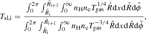
where  is the azimuthal angle in the plane of the sky, ne(r) and nH(r) are the electron number density of the ICM and the equivalent number density of the hydrogen nuclei, respectively, and C = 10−14/[4πDang2(1+z0)2], with Dang and z0 the angular distance and systemic redshift of the cluster, respectively, is the normalization factor adopted in XSPEC. In our analysis we compared our models with the quantity
![$$ \begin{aligned} {\mathcal{N} }_{\mathrm{i}}= \frac{Norm_{\mathrm{i}}}{\pi \left[\left({\hat{R}}_{\mathrm{i + 1} }/[\mathrm{arcmin}]\right)^2 - \left(\hat{R}_{\mathrm{i} }/[\mathrm{arcmin}]\right)^2\right]}, \end{aligned} $$](/articles/aa/full_html/2025/05/aa53720-25/aa53720-25-eq8.gif)
whose values are provided by G19.
2.2. ICM thermodynamic properties from the SZ effect
We present here the properties of the X-COP clusters as inferred from the SZ effect signal in the Planck maps by G19 and reported in the X-COP website.
G19 analyzed the Compton y-parameter maps, under the assumption that the relation between the “SZ pressure”, PSZ, and the y-parameter in Eq. (3) of G19 holds. Radial profiles were extracted in Nbins,SZ circular bins, and then deconvolved by the Planck PSF and geometrically deprojected under the assumption of spherical symmetry. It follows that they recovered the SZ pressure as the average in the j-th spherical shell with radii rj and rj + 1, PSZ,j, where j = {1, …, Nbins,SZ} (see Sect. 2.5 of G19, for details). In this analysis, a covariant matrix accounts for the errors and the cross-correlations between the values of PSZ,j at all j. Given that the diagonal terms of the covariance matrix are dominant, we neglected the off-diagonal terms and considered only the errors from the diagonal terms in the model-data comparison. Given that the sizes of the three central radial bins in PSZ,j, as widely discussed in G19, are smaller than the PSF of Planck, we excluded them from the model-data comparison. The used PSZ data range from ∼0.5r500 out to ∼3r500 in all the clusters.
2.3. Cluster mass distribution
The spherically averaged mass density profile of the observed clusters and those formed in cosmological simulations are routinely described by the virial mass M200 and by the concentration c200 = r200/r−2, where r−2 is the radius at which the logarithmic slope of the density profile is −2.
We took the distribution of M200 measured from WL analysis, when available, as the reference estimate of the cluster mass. Specifically, we took from Col. 4 of Table A.2 of Herbonnet et al. (2020) the average and the 1σ scatter of WL mass estimates for the clusters A85, A1785, A2142, and Zw1215. These values defined our a priori normal distribution of M200 for each of these clusters. For the remaining clusters, we assumed the a priori normal distribution of M200 as follows. We took the median of the M200 from Table 2 in Eckert et al. (2019), who estimated the M200 distributions of each cluster of the X-COP sample using a correction for the hydrostatic masses based on the assumption of the universal baryon fraction. We conservatively adopted as the standard deviation (normalized to the median M200) σ = (σubf2+σWL2)1/2, where σubf is (for each cluster) the average between the upper and lower relative uncertainties on M200 (taking the data from Table 2 of Eckert et al. 2019), and σWL is the average relative uncertainty on WL estimates of M200 for the aforementioned five clusters with WL measurements.
We assumed a Gaussian prior distribution of lnc200. For each cluster the median lnc200 is obtained from the median M200, using the mass-concentration relation in Eq. (5) of Ragagnin et al. (2021), with coefficients given by their Eq. (7) evaluated for the cosmological parameters adopted in this work. Following Ragagnin et al. (2021), for all clusters we assumed 0.38 as the standard deviation of the prior distribution of lnc200.
3. Models for a pressure-supported rotating ICM
We present here two families of axisymmetric cluster models with rotating ICM that we applied to our sample of clusters: in one family the ICM is assumed to have no turbulence, while in the other the turbulence of the ICM is accounted for. Models without turbulence, though idealized, are interesting, because they allow us to estimate the maximum room for rotation in the ICM, and could be not too unrealistic, if the negligible turbulence support, measured in the central regions of the Perseus cluster and A2029 (Hitomi Collaboration 2016; Miller et al. 2025), is confirmed at larger distances from the center and in other clusters.
Both families belong to the class of models presented by B24 (see also Bianconi et al. 2013; Nipoti et al. 2015), in which a pressure-supported and rotating ICM has a composite polytropic distribution (e.g., Curry & McKee 2000) and is in equilibrium in the gravitational potential of a dark-matter halo (the self-gravity of the gas is neglected). While B24 considered also oblate and prolate dark halos, here, for the sake of simplicity, we limited ourselves to the case of spherical dark halos: in particular, we adopted a spherical Navarro-Frenk-White (NFW; Navarro et al. 1996) gravitational potential, which is fully determined by the parameters M200 and c200 (see, e.g., Sect. 2.2 of B24). We generalized the formalism of B24 by interpreting the gas pressure p as
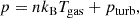
where n is the gas number density and pturb is the turbulent pressure, which we parameterized as pturb = αturbp, with αturb = αturb(p) a dimensionless quantity in the range 0 ≤ αturb < 1, representing the fraction of turbulent pressure support. The ICM temperature is thus given by
3.1. Intrinsic properties of the models
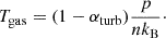
Here we describe the intrinsic properties of the models adopting a cylindrical coordinate system (R, ϕ, z). Given that the gas distribution is barotropic, the gas rotation velocity uϕ depends only on R: as in B24, we assumed
where S ≡ R/Rpeak, Rpeak is the radius at which uϕ is maximum and5upeak ≡ uϕ(Rpeak). This functional form of uϕ(R) is relatively flexible and is able to reproduce the average rotation velocity profiles of the ICM found in cosmological simulations for clusters with masses comparable to those of X-COP clusters (see B24).
In the composite polytropic models here adopted, the gas number density distribution is
![$$ \begin{aligned} n(R,z)=n_\star \left[1- \frac{\gamma \prime -1}{\gamma \prime } \frac{n_\star \mu m_{\rm p}}{p_{\star }} \Delta \Phi _{\mathrm{eff}}(R,z)\right]^{\frac{1}{\gamma \prime -1}}, \end{aligned} $$](/articles/aa/full_html/2025/05/aa53720-25/aa53720-25-eq12.gif)
and the pressure distribution is
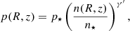
with γ′=γ′IN and γ′=γ′OUT in the inner and outer regions of the cluster, respectively. The effective potential Φeff, depending on M200, c200, upeak and Rpeak, is defined in Eqs. (24) and (25) of Bartalesi et al. (2024). In the above equations, n⋆ = n(Rbreak, 0) and p⋆ = p(Rbreak, 0), with Rbreak the radius in the equatorial plane where the value of the polytropic index changes; μ is the mean molecular weight and mp is the proton mass. We assumed a position-independent metallicity of 0.3 times the solar value, for which μ = 0.6 and n/ne = 1.94, or ne = 1.17nH in a fully ionized plasma. For models both with and without turbulence, we found it convenient to define the parameter T⋆ ≡ p⋆/(n⋆kB), which is the gas temperature at (Rbreak, 0) when αturb = 0 and can be interpreted as an equivalent gas temperature at (Rbreak, 0) when αturb ≠ 0.
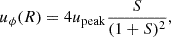
In models with turbulent ICM (0 ≤ αturb < 1) we adopted the following law to describe the dependence of αturb on p:
![$$ \begin{aligned} \alpha _{\mathrm{turb}}(p) = (\alpha _{\mathrm{inf}}- \alpha _0) \frac{\ln \left[1 + p/(\xi p_\star )\right]}{p/(\xi p_\star )} + \alpha _0, \end{aligned} $$](/articles/aa/full_html/2025/05/aa53720-25/aa53720-25-eq14.gif)
where ξ is a dimensionless parameter. In Eq. (8), α0 and αinf are the asymptotic values of αturb for p ≫ ξp⋆ and p ≪ ξp⋆, respectively (the transition between the two regimes occurs where the pressure has values around ξp⋆). Given that, for a pressure-supported cluster, the pressure decreases outward, αturb increases outward if αinf > α0. The contribution to the ICM support against cluster gravity from turbulent motions is routinely measured as a spherically averaged αturb profile in clusters formed in cosmological simulations. Using a multi-scale filtering technique (see Vazza et al. 2012), which is believed to isolate the uncorrelated component of the velocity field of the ICM, Angelinelli et al. (2020, hereafter A20) accurately estimated the profiles of αturb for a sample of 68 clusters formed in a cosmological, non-radiative simulation without active galactic nucleus or stellar feedback. They, then, presented a functional form in their Eq. (11) that successfully reproduces the outward increasing radial dependence of the median αturb profile of these clusters. The functional form of αturb presented in Eq. (8) is thought to generalize that of A20 to nonspherical analyses, in particular to axisymmetric systems for the scope of this work.
In summary, the family of models without turbulence (αturb = 0) has 9 free parameters: γ′IN, γ′OUT, n⋆, T⋆, Rbreak, M200, c200, Rpeak, and upeak. The family of models with turbulence has 12 free parameters: αinf, α0 and ξ, in addition to the nine parameters of the other family.
3.2. From models to observational data
We define here the quantities, obtained from the intrinsic properties of our models (see Sect. 3.1), that can be compared with the observational data detailed in Sect. 2. We use the Cartesian reference system and the radial grids  and rj introduced in Sect. 2.
In the apec emission code, Tsp is formally the temperature of an isothermal emitting plasma (see Sect. 2.1). Given that the ICM in our model is multi-temperature, we adopted, as an approximation of Tsp, the spectroscopic-like temperature Tsl (see Mazzotta et al. 2004, for details) so that we could compare the Tsl derived from our models to Tsp. Tsl in the i-th cylindrical shell, with radii  and
and  , is
, is
where Tgas is the intrinsic temperature of the ICM. The SZ pressure, obtained from the intrinsic properties of the ICM in our models, is assumed to be the average of the thermal pressure distribution of the ICM in the j-th spherical shell, with radii rj and rj + 1,
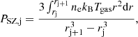
where r is the spherical radius and kB the Boltzmann constant.
In the comparison between the models and the observed dataset, we assumed that our axisymmetric models are observed edge-on, that is, with line of sight x orthogonal to the symmetry and rotation axis z. As we have seen in Sect. 2, the observational data we want to compare with are measurements of quantities in either circular annuli or in spherical shells centered in the cluster center. Though we could perform analogous measurements for our models starting from Eqs. (1), (9), and (10), in order to save computational time in the model-data comparison, we approximated such measurements with estimates obtained by considering only properties of the models in the equatorial plane (z = 0). The details of this approximation, which turns out to be sufficiently good for our purposes, are given in Appendix D. In particular, imposing that the gas density is zero when |x|> rNSZ or |y|> rNSZ, where rNSZ is the outer radius of the outermost spherical shell, we applied the approximations (D.3) and (D.4) to our models. Thus, Eqs. (1) and (9) become, respectively,
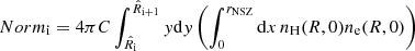
and
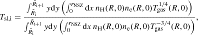
with  ; Eq. (10) becomes
where η is a parameter accounting for the possible systematic offset between the electron pressure of the ICM and that measured from the Compton y-parameter maps (see Appendix A).
4. The statistical method
For each cluster of our sample we computed both αturb = 0 and αturb ≥ 0 models. Taking mass distributions based on available estimates (see Sect. 2.3), these models, presented in Sect. 3, are tuned to reproduce the radial profiles of 𝒩, Tsp and PSZ as resolved in the XMM-Newton and Planck maps (see Sects. 2.1 and 2.2) via a Markov chain Monte Carlo (MCMC) method. This section details the statistical method: we present the form of the likelihood and the prior distributions in Sects. 4.1 and 4.2, respectively, and the method used to estimate the posterior distribution of the model in Sect. 4.3. The details of the MCMC algorithm are described in Appendix B.
4.1. Likelihood
Using the models described in Sect. 3, we reconstructed the intrinsic properties of the ICM (density, turbulent and thermal pressures, and rotation speed) and the gravitational potential in which it is in equilibrium. From the model of the intrinsic quantities of the ICM, we evaluated the radial profile of 𝒩, Tsl and PSZ as described in Sect. 3.2 (we recall that the normalization of the PSZ profile is regulated by η, which is one of the free parameters of the MCMC). The statistical errors, σstat, on the observed 𝒩, Tsp and PSZ are obtained as the average between the upper and lower 1σ errors reported in the data analyses. We considered three parameters, ϵN, ϵT, and ϵSZ, to account for a systematic contribution, ϵσstat with ϵ = {ϵN, ϵT, ϵSZ}, to the uncertainty in the values of 𝒩, Tsp and PSZ, respectively. ϵN, ϵT and ϵSZ are assumed to have the same values in all the radial bins. Specifically, we assumed each datum of 𝒩, Tsp and PSZ to be randomly generated from a normal distribution with a median equal to the corresponding 𝒩, Tsl and PSZ in the model and a standard deviation equal to  . It follows that the generic likelihood of each datum Qm, im, ℒ(Qm, im), where Qm with m = {1, 2, 3} indicates 𝒩, Tsp, or PSZ, respectively, and im the radial bin in which Qm was extracted, is a normal distribution with the same median and standard deviation as described above. The radial bins used in the fitting are defined in Sects. 2.1 and 2.2.
4.2. Prior distributions
Let us consider the marginal prior of the generic parameter θh, π(θh), where h = {1, …, H} with H the number of the parameters in the fitting. We found it convenient to use ν⋆ ≡ log[n⋆/(10−3 cm−3)] as the MCMC parameter instead of n⋆. In addition to the parameters of the models (see Sect. 3.1), for the joint analysis of the X-ray and SZ data we introduced the four parameters η, ϵN, ϵT and ϵSZ (see Sect. 4.1), so for the αturb = 0 models we have H = 13 parameters (γ′IN, γ′OUT, ν⋆, T⋆, Rbreak, log ϵN, log ϵT, upeak, Rpeak, η, log ϵSZ, M200, and lnc200), while for the αturb ≥ 0 models we have H = 16 parameters (log ξ, αinf and α0, in addition to those of the αturb = 0 models).
We assumed π(M200) and π(lnc200) to be Gaussian, with the medians and standard deviations reported for each cluster in Table 1 (see also Sect. 2.3). For all the other parameters we assumed a uniform prior distribution, with upper and lower bounds reported in Table 2. The choice of the upper and lower bounds of the parameters regulating the turbulent support (log ξ, α0 and αinf) requires a brief comment. The parameter log ξ sets the distance from the center where there is a transition between an inner region (p ≫ ξp⋆) in which αturb → α0 and an outer region (p ≪ ξp⋆) in which αturb → αinf. We adopted a prior on log ξ uniform in the range [−1.5, 0]. This is motivated by the expectation (based on the properties of the SRM model from B24) that values of log ξ in the range [−1.5, 0] map the radial range (0.15−1)r200, which ensures the transition does not occur within the cluster core (log ξ = 0 sets the transition in the αturb profile at R ≈ Rbreak in the equatorial plane). For our models applied to the X-COP clusters, a turbulent velocity dispersion higher than σRGS = 500 km s−1 at a distance smaller than ≈150 kpc would violate the 90% upper limit on the broadening of the X-ray emitting lines from RGS data. We thus set the upper bound of π(α0) to α0,RGS = σRGS2/[σRGS2+kBT0/(μmp)], where T0 is the best-fit observed spectroscopic temperature in the innermost annulus of each cluster (taken from G19). αinf accounts for the turbulent support at large radii, which is observationally unconstrained. We thus assume 0.95 as upper bound of π(αinf), which corresponds to dominant turbulent pressure in the outskirts (see Sect. 3.1). We set the lower bounds of π(α0) and π(αinf) to 0, to conservatively include the possibility of negligible turbulence.
Lower and upper bounds of the uniform prior distributions of the MCMC parameters γ′IN, γ′OUT, ν⋆, T⋆, Rbreak, log ϵN, log ϵT, upeak, Rpeak, η, and log ϵSZ (common to models both with and without turbulence), and of the parameters log ξ, αinf, and α0 (used only in the model with turbulence).
4.3. Posterior distributions
According to Bayes’ theorem, the posterior distribution of the parameter vector θ = (θ1, …, θH), 𝒫(θ), is obtained from ![$ \ln {\mathcal{P}}= \sum_{h = 1}^{H} \mathcal \ln \left[\pi(\theta_{h})\right] + \sum_{m = 1}^{3} \sum_{i_{m}} \ln \left[\mathcal{L}(Q_{i_m})\right] $](/articles/aa/full_html/2025/05/aa53720-25/aa53720-25-eq25.gif) , where π(θh) and ℒ(Qm) are described in Sects. 4.1 and 4.2, respectively. The MCMC algorithm individually maximizes ln𝒫 of each cluster. When it converges to a stationary posterior, we obtain the discrete posterior consisting of a sample of the parameter vector (see Appendix B for details). The relative frequency of the values of the parameters in this sample can be visualized in corner plots, which we present for the parameters M200, lnc200, upeak, Rpeak and α0 (if αturb ≠ 0) for all clusters in Appendix E.
, where π(θh) and ℒ(Qm) are described in Sects. 4.1 and 4.2, respectively. The MCMC algorithm individually maximizes ln𝒫 of each cluster. When it converges to a stationary posterior, we obtain the discrete posterior consisting of a sample of the parameter vector (see Appendix B for details). The relative frequency of the values of the parameters in this sample can be visualized in corner plots, which we present for the parameters M200, lnc200, upeak, Rpeak and α0 (if αturb ≠ 0) for all clusters in Appendix E.
We chose to characterize the marginal posterior distributions using the 68% HPDI as a credible interval (see Sect. 1), which is very similar to the interval between the 16th and 84th percentiles for symmetric distributions, but tends to be more meaningful than the 16th and 84th percentiles for highly skewed distributions. For the sake of conciseness, in the following we refer to the lower and upper bounds of the 68% HPDI credible interval on the marginal posterior distribution on a parameter, simply as the lower and upper limits on that parameter.
For each parameter vector belonging to our sampling of the posterior distribution (see above), we computed a few relevant quantities for each cluster, needed for the interpretation of the results presented in Sect. 5. In particular, we derived the profiles of 𝒩, Tsl and PSZ as described in Sect. 3.2, and the rotation curve using Eq. (5). The 1D velocity dispersion of the gas particles at a given point in the equatorial plane is given by ![$ {\sigma_{\text{gas,1D}}}(R, 0) = \sqrt{p(R, 0)/\left[\mu {m_{\text{p}}}n(R, 0)\right]} $](/articles/aa/full_html/2025/05/aa53720-25/aa53720-25-eq26.gif) . As a measure of the dynamical importance of rotation, we computed, as a function of radius R, the ratio between the gas rotation velocity uϕ(R) and the gas velocity dispersion σgas,1D(R, 0) in the equatorial plane, uϕ/σgas,1D. Given that we are interested in the effect of the turbulence when fitting the thermodynamic data with a rotating ICM model, in the αturb ≥ 0 models, we also derived the αturb(p) profile through Eq. (8) once we had obtained the pressure profile (see Sect. 3.1). The 1D turbulent velocity dispersion in the equatorial plane is then given by
. As a measure of the dynamical importance of rotation, we computed, as a function of radius R, the ratio between the gas rotation velocity uϕ(R) and the gas velocity dispersion σgas,1D(R, 0) in the equatorial plane, uϕ/σgas,1D. Given that we are interested in the effect of the turbulence when fitting the thermodynamic data with a rotating ICM model, in the αturb ≥ 0 models, we also derived the αturb(p) profile through Eq. (8) once we had obtained the pressure profile (see Sect. 3.1). The 1D turbulent velocity dispersion in the equatorial plane is then given by  , where p = p(R, 0).
In Appendix E we show for each cluster the profiles of 𝒩, Tsl, and PSZ for the αturb = 0 model. The 𝒩, Tsl and PSZ profiles of the αturb ≠ 0 models, not shown, are virtually indistinguishable from the corresponding profiles of the αturb = 0 models. We also show for each cluster the uϕ profile of the αturb = 0 model, and the uϕ/σgas,1D and αturb profiles of the αturb ≥ 0 model.
5. Results
We present here the results obtained by applying our models, presented in Sect. 3, to the observed thermodynamic profiles of the X-COP objects through the statistical method described in Sect. 4, focusing in particular on the radial distribution of the ICM rotation and turbulence.
5.1. Models of rotating ICM without turbulence
Our models are able to closely reproduce the observed properties of the ICM (Sect. 2) of all the clusters of our sample from a radius comparable to the brightest cluster galaxy size out to ∼3r500, the outermost radial bin in the PlanckPSZ profile (see Appendix E). The residuals between the median of the model and the data are, as a rule, not larger than 6% in the radial profiles of 𝒩, Tsp and PSZ (the only exceptions are A644 and A2319, for which the residuals are between 6% and 10%). The median value of ϵN inferred in the sample is 4.5 (the median ϵN in each cluster ranges from 1, in Zw1215, to 10, in A85). The values of ϵT and ϵSZ are lower than 1 in all the clusters of the sample, apart from the ϵT in A644, A1644, and A2319, whose medians range from 2 to 4. The median errors inferred as  are plotted in the thermodynamic profiles in Appendix E.
For all the clusters, the posterior distribution 𝒫 of upeak is unimodal, with a credible interval that encloses the mode (see the corner plots in Appendix E). In most cases, the range between the lower and upper limits of upeak is wide, implying that the uncertainty on the inferred values of upeak is large. The posterior lower limit of upeak is very close to the lower bound of π(upeak), except for three clusters (A1795, A2255, and A2319).
Considering our full sample of objects, we characterized the distribution of the profiles of any quantity, say q(R), by defining 1σ lower and upper limits of as follows. At any radius R in the equatorial plane, we define the 1σ lower limit as the median of the 16th percentiles of the distribution of q evaluated at R in each cluster model. The 1σ upper limit is defined in the same way, but by taking the 84% percentiles.
Figure 1 summarizes the rotation properties of our models of the clusters of our sample. In the left panel, we show the median uϕ/σgas,1D profiles of the clusters (see Sect. 4.3). A common trend emerges: this population of clusters exhibits a slightly outward-increasing median profile of uϕ/σgas,1D. However, the lower limit of the population (lower bound of the gray band in the plot) has everywhere uϕ/σgas,1D < 0.2, corresponding to ρuϕ2/p < 0.04, which indicates a negligible rotation support. In the right panel, where we show the median profiles of the rotation velocity in the cluster models, the lower limit of the population (lower bound of the gray band in the plot) corresponds to velocity everywhere below 100 km s−1. The population upper limit of the uϕ/σgas,1D profile (upper bound of the gray band in the left panel) significantly increases outward up to nearly 0.9 (corresponding to a rotation velocity of ≈600 km s−1; see the right panel).
Taking the difference between the population upper and lower limits as a measure of the 1σ scatter, we find that the scatter in uϕ/σgas,1D and in uϕ is up to 0.7 and 500 km s−1, respectively, implying that the determination of the properties of the population in our models is very uncertain. Three clusters have median uϕ/σgas,1D and uϕ profiles significantly higher than the 1σ upper limit of the population: A1795 and A2319 have high uϕ/σgas,1D and uϕ in the outskirts (with uϕ higher than 1000 km s−1), while A2255 at intermediate radii (with uϕ ≈ 500 km s−1).
We conclude that, if turbulence in the ICM is negligible throughout the cluster (which is an hypothesis consistent with the currently available measurements in the central regions of the Perseus cluster and A2029; Hitomi Collaboration 2016; Miller et al. 2025), the current data of the X-COP clusters leave room for an important rotation in the ICM (especially in the three clusters A1795, A2319 and A2255), even if in most cases they are also consistent within the 68% credible interval with negligible rotation of the ICM.
In the next section we consider the case in which the contribution of ICM turbulence is accounted for in the models.
5.2. Models of rotating ICM with turbulence
When applying the αturb ≥ 0 model to the clusters of our sample, we find that the posterior distributions of the parameters γ′IN, γ′OUT, ν⋆, Rbreak, log ϵN, log ϵT, η, log ϵSZ, M200 and lnc200 are very similar to the case of the αturb = 0 model. We find instead significant differences in the posterior distributions of the parameters T⋆, upeak and Rpeak. This confirms the expectation that the X-ray and SZ data alone are insufficient to distinguish between the two forms of nonthermal support considered in our study. However, the functional forms adopted for the radial profiles of rotation and turbulence play a pivotal role in separating the rotational contribution to nonthermal support from that from turbulence. In all the clusters, the upper limit of upeak for αturb ≥ 0 tends to be lower than for αturb = 0, which indicates that rotation is less important when the ICM is turbulent. This is expected, because turbulence contributes to the pressure support against gravity, thus reducing the room for rotational support.
Figure 2 summarizes the properties of the αturb ≥ 0 models for the clusters of our sample. As shown in the upper-left panel, when αturb ≠ 0 the population upper limit on uϕ/σgas,1D (upper bound of the gray band in the plot) is ≈0.6 (corresponding to a rotation speed of ≈500 km s−1; see the upper-right panel), smaller than ≈0.9 found when αturb = 0, but still indicating room for significant rotation support, even in the presence of turbulence. Conversely, as shown in the lower panels of Fig. 2, the 1σ scatter of the turbulent-to-total-pressure ratio (αturb, in its left panel) and 1D turbulence velocity dispersion (σturb,1D, in its right panel) in the population ranges from ≈0.05 and 200 km s−1 up to 0.4 and 500 km s−1, characterized by a very significant rise of population upper limit of αturb in the outskirts.
It is particularly interesting to compare αturb = 0 and αturb ≥ 0 models of the clusters whose αturb = 0 model shows significant rotation, namely A1795, A2319, and A2255. The models of A1795 and A2319 have similar properties. The αturb = 0 models of both objects have a posterior lower limit of upeak around 850 km s−1, much higher than the lower bound of the prior of upeak (see the corner plot in Figs. 4 and 7 of Appendix E, respectively). This corresponds to a median uϕ/σgas,1D exceeding 1 in the outskirts and thus significantly deviating from the average properties of the population (see the right panel of Fig. 1). Instead, when αturb ≥ 0, the models of A1795 and A2319 have posterior lower limit of upeak coincident with the lower bound of π(upeak) (50 km s−1). This translates into a median uϕ/σgas,1D profile, with a value below 0.4 in the outskirts, that everywhere falls within the 1σ interval of the population (see the upper-left panel of Fig. 2). The lower-left panel of Fig. 2 shows the median turbulent-to-total pressure ratio profile αturb(R) of our clusters. A1795 and A2319 have αturb significantly increasing outward, with αturb > 0.5 in the outskirts, standing out from the 1σ band of the considered cluster population. We can interpret this as a significant shift of the nonthermal support from rotation to turbulence in the outer regions.
In the αturb ≥ 0 model, A2255 exhibits the highest median uϕ/σgas,1D profile in a region close to the center, making it the most promising candidate for detecting rotation in the ICM with XRISM/Resolve. The credible interval of 𝒫(upeak) in the αturb ≥ 0 model consists of two separate intervals corresponding to relatively low and high values of upeak, centered at 100 km s−1 and 600 km s−1, respectively. 𝒫(upeak) is relatively flat, from the lower bound of the low-upeak credible interval (that is the lower bound of the prior) to the upper bound of the high-upeak credible interval, which is approximately equal to the 1σ upper limit of upeak in the αturb = 0 model. Given the relatively high rotation velocity of the ICM in the inner or intermediate regions, this cluster warrants further investigation through a dedicated XRISM pointing in its center. In Sect. 5.4 we propose an observational strategy with XRISM/Resolve to validate the rotation peak of 500 km s−1 at a distance of 200 kpc from the center.
In Appendix C we compare the flattening of the X-ray surface brightness distribution measured in our models with the measurements of the X-COP clusters. We found that the αturb = 0 models (being more flattened) tend to perform better than the αturb ≥ 0 models in reproducing the observed distribution of the axial ratios estimated from the X-ray maps. This might indicate that the ICM turbulence support is not as high as inferred with our analysis. However, it must be stressed that in our models, where the gravitational potential is spherically symmetric, only the rotation determines the flattening of the X-ray surface brightness distribution. The flattening of the ICM can also be influenced by the shape of the dark-matter halo, which can deviate significantly from spherical symmetry (e.g., Allgood et al. 2006). This is widely discussed in B24, where models of the rotating ICM in equilibrium in both prolate and oblate halos were studied.
5.3. Comparison with the published studies on ICM motions
To our knowledge, the present work is the first attempt to reproduce the temperature, density and pressure profiles of the observed clusters with models with rotating and turbulent ICM, consistent with the available mass estimates. Here we compare our results with published works presenting constraints on the contribution of nonthermal pressure support from observed datasets, where the nonthermal component is totally ascribed to turbulence, and on the turbulent support in clusters formed from cosmological hydrodynamic simulations.
Ettori & Eckert (2022, hereafter E22) present constraints on the contribution of a nonthermal component to the total pressure, which is assumed to be in hydrostatic equilibrium in the gravitational potential of the X-COP clusters. The nonthermal pressure is parametrized as a power-law dependence upon the gas density with the normalization and the slope as free parameters. These free parameters are constrained by requiring that the gas mass fraction at an overdensity of 500 and 200 ρcrit matches a “universal” value, which was derived from cosmological simulations, accounting for the baryonic mass fraction and subtracting a statistical contribution for stellar mass (see also Eckert et al. 2019). By construction, the model is sensitive to the regions where a gas mass fraction measurement (based on the initial assumption that the total pressure support is only thermal) is available, and it can only account for nonthermal pressure support in systems where the observed gas fraction exceeds the universal value.
For the sake of simplicity, we compare our αturb = 0 rotation velocity profile, which contains the entire information on the nonthermal support, with the 1D turbulent velocity dispersion profiles obtained in E22 for the same cluster (see their Eq. 21). In the regions where the gas mass fractions are available (r ∼ r500 − r200), the 1D turbulent velocity dispersion profiles of E22 for most clusters lies within the range between the 16th and 84th percentiles of our reconstructed rotation velocity profiles. However, in A1795 the 1D turbulent velocity dispersion profile from E22 is significantly lower than the 16th percentile of our rotation velocity profile. Although a detailed investigation of the cause of this discrepancy is beyond the scope of this comparison, we suggest a potential inconsistency in the mass estimates6 rather than issues related to the different modeling. Overall, in E22, A2255 and A2142 show a central 1D velocity dispersion of about 400 km s−1, and are therefore promising candidates for a detectable ICM rotation. While A2142 was found with low nonthermal support in the central regions in our model (see the left panel of Fig. 1), we confirm the high level of nonthermal support near the center of A2255.
In B24, we compared the rotation curves of our models with those recovered from some cosmologically simulated clusters. Given that the inferred constraint on the turbulence in our models impacts the inferred rotation, we investigate here how our constraints on the turbulent component of the ICM velocity field relate to the predictions of A20, who accurately recovered the turbulent part of the ICM velocity field in their simulated sample (see Sect. 3.1, for details). In the lower-left panel of Fig. 2, we overlay the median profile of αturb from A20. This average profile is well in agreement with our median results, lying within the interval between the 16th and 84th percentiles of the distribution of the αturb profiles in the X-COP population from ∼50 kpc out to ∼3r500, although local tensions in specific cases are expected and observed (see the plots in Appendix E).
 |
Fig. 1. Equatorial plane velocity profiles of the ICM in the αturb = 0 models of the clusters of our sample. Left panel: Ratio between the gas rotation velocity and velocity dispersion (measured in the equatorial plane) as a function of the cylindrical radius normalized to the virial radius, r200 = 3M200/[800πρcrit]1/3, computed using the median value of M200 for each cluster. Right panel: Gas rotation velocity as a function of the cylindrical radius in physical units. In both panels the dashed lines are the median profiles of the individual clusters (as indicated in the legend), whereas the gray band represents the interval between the 16th and 84th percentiles of the distribution of the profiles of the entire sample of clusters. |
 |
Fig. 2. Equatorial plane rotation and turbulence profiles of the ICM in the αturb ≠ 0 models of the clusters of our sample. Upper panels: Same as Fig. 1 but for models with αturb ≥ 0. Lower left panel: Median turbulent-to-total pressure ratio, αturb, as a function of the cylindrical radius normalized to the virial radius, r200 (see the caption of Fig. 1), for the same models as in the upper panels. Lower right panel: 1D turbulent velocity dispersion as a function of the cylindrical radius in physical units for the same models as in the upper panels. The color coding and the meaning of the gray bands are the same as in Fig. 1. In the lower right panel, we overplot the αturb profile measured in simulations by A20 (solid black line; the profile was taken from their Eq. (11), with a0, a1, and a2 equal to their best-fit values, as reported in the first row of their Table 1, and assuming r200, m/r200 ≈ 1.67). |
5.4. Detecting the ICM rotation with XRISM: Abell 2255
In this section we study the capability of high-resolution (eV-scale) X-ray spectroscopy to detect and characterize the rotation of the ICM. In particular, the X-ray calorimeter Resolve on board the XRISM mission7 is the only currently available instrument that can offer such a spectral resolution; however, it has a limited collecting area and FoV, meaning it can only efficiently capture the brightest regions. In B24, we studied the significance of the measurement of the rotation through the estimates of the centroid of the iron emission lines, the impact of the line broadening on these estimates and its cross-correlations with the other fitting parameters in the analyses of a set of XRISM/Resolve mock spectra generated from three realistic (but generic) rotating ICM models. Here, we present a feasibility study applied to A2255, the most interesting target because of its highest median rotation velocity (≈500 km s−1 as inferred from the αturb ≠ 0 model) near the center in the considered sample of objects.
A2255 is a disturbed, non-cool-core system at redshift z0 = 0.0809, settled in the North Ecliptic Pole SuperCluster. It shows a flat X-ray surface-brightness profile in its core and an X-ray morphology extended along the E–W axis (Sakelliou & Ponman 2006), which could indicate the presence of rotation. Spectral analysis of XMM-Newton data shows that the temperature distribution presents azimuthal variations. These characteristics were interpreted as due to a shock moving along the E–W direction with Mach number ∼1.24 and with a core crossing occurred ∼0.15 Gyr ago (Sakelliou & Ponman 2006). Also, some properties inferred from multiwavelength observations, such as the fact that the X-ray centroid of the cluster does not coincide with the position of the brightest galaxy, are consistent with the merger scenario (Burns et al. 1995). While there is currently no solid evidence of a radio counterpart of E–W shock, many relics were detected in the outskirts (some seen in projection), and a radio halo was detected in the center (Pizzo et al. 2008; Pizzo & de Bruyn 2009). Recent deep radio observations of A2255 suggested that very composite mechanisms, including seed particles injected by radio galaxies and spread in the ICM by turbulent motions and weak shocks, are at work at the same time to generate the radio halo (Botteon et al. 2020, 2022). Interestingly, Roettiger & Flores (2000), using a hydrodynamical N-body simulation, found that off-axis mergers are an efficient mechanism for transferring angular momentum to the ICM, which suggests that large-scale rotation of the ICM could be present in post-merging objects (see also Roettiger et al. 1998).
We simulate a pointing with XRISM/Resolve centered on the core of A2255 and including a rotation speed of 500 km s−1. When we extract a spectrum from the entire FoV of Resolve, consisting of 6 × 6 pixels covering an area ≈3 × 3 arcmin2, and affected by a PSF with a half-power diameter of about 1.3 arcmin (≈130 kpc, at the redshift of A2255), both turbulent and rotational motions would contribute to the measured broadening of the X-ray emission lines. To associate the rotation with the shifting of the centroids of the X-ray emitting lines and decouple it from the turbulent motions in the ICM, we consider the following observational strategy. We assume that, if the ICM rotation is present in the Resolve exposure, it can be resolved by looking at the different redshift measured in two complementary spectra extracted from the single observation. To evaluate this, we divide the FoV into two complementary sectors of 3 × 6 pixels. We simulate the ICM emission using the thermal plasma emission model bapec8 with a 6.2 keV temperature, the value spectroscopically measured with an XMM exposure of the central regions (see G19) and abundance equal to 0.3 times the solar abundance in Anders & Grevesse (1989) (see Ghizzardi et al. 2021, for details). The normalization is set to the fraction (∼20%) of the 0.5−2 keV band luminosity estimated within the hydrostatic r500 that falls within the Resolve FoV using a β model (Cavaliere & Fusco-Femiano 1978) with parameters the scale radius rc = 0.15r500 and the exponent β = 0.65. Given that we are considering half of the Resolve FoV, the normalization of the bapec model is defined as half of the estimated flux. In the simulated spectrum, the nominal redshift z0 is modified as  (Roncarelli et al. 2018), where c is the light speed. Given that the peak of the rotation lies within the 3 × 6 sector, in this equation we considered the peak rotation velocity, upeak (positive for a receding ICM). For z0 = 0.0809 and upeak ∼ ±500 km s−1, zu = 0.0791 and 0.0827, respectively. The most prominent emission line complex, key to accurately recovering the redshift of the ICM, is that of iron (Fe XXVI) at rest-frame energy equal to 6.7 keV. The centroid of it should be shifted, in the observer’s frame, to (6.188, 6.199, 6.209) keV for a rotation of +500, 0, −500 km/s, respectively. These values correspond to differences in the locations of the Fe XXVI lines of ΔE ≈ 10 − 21 eV that cannot be resolved with CCD-like spectral resolution (like for XMM), but are well above the Resolve spectral resolution and accuracy of about 4.8 and 0.2 eV, respectively. We include a broadening of the X-ray emission lines equal to the median turbulent velocity dispersion (≈300 km s−1) inferred from our model. All the spectra are absorbed by the expected Galactic column density of 2.5 × 1020 cm−2. This parameter is kept fixed in the following spectral analysis. Using the responses for the closed Gate-Valve configuration, and adding an instrumental and a cosmic background and a Poissonian noise, we simulate in XSPEC the 1.8−10 keV spectrum of the rotating ICM, as shown in Fig. 3. Importantly, the instrumental background is significantly lower than the thermal model, and the cosmic background adds a relatively small contribution to the flux of the 6.1−6.2 keV emission line complex. We proceed by fitting the broadband (1.8−10 keV) spectrum, fixing the best-fit value of the temperature, and fitting the region around the Fe XXV–XXVI complex again. We obtain that a minimum exposure of 100 ks is required to reach accuracy and precision of < 1% on the measurement of the redshift, allowing us to identify the centroid of the redshifted emission lines at more than 5σ level of confidence for a rotation greater than ±400 km s−1 (ΔE ≈ 17 eV), and at > 3σ for a rotation down to ±200 km/s (ΔE ≈ 8.2 eV). The temperature, line broadening and metallicity are consistently measured with an accuracy on the order of 10−20%. The PSF is not an issue when determining the centroid of the emitting lines in two different sectors. Moreover, based on the analysis of the spectral simulations presented in B24, no significant cross-correlation between the bapec parameters affects our reconstruction, which assures us that it is possible to find evidence of a rotating ICM in A2255.
 |
Fig. 3. Simulated spectrum (black crosses), with an exposure of 100 ks, in half of the Resolve FoV with the best-fit bapec model overplotted. The thermal model only is shown with the green line, the instrumental background in blue, and the thermal model plus the instrumental and cosmic background in red. The most prominent lines are the Fe XXV and Fe XXVI complexes in the range 6−7 keV. |
6. Conclusions
We have presented equilibrium models with a rotating ICM for 11 galaxy clusters from the X-COP sample. In the models, based on those of B24, the gas has an axisymmetric composite polytropic distribution, in equilibrium in the gravitational potential of a spherical NFW dark-matter halo. For each cluster we considered both the case of a turbulent ICM (αturb ≥ 0) and the case of an ICM with negligible turbulence (αturb = 0). The profile of rotation velocity and the distribution of turbulent velocity dispersion are described with flexible functional forms that are able to reproduce the radial profiles obtained from the spherically averaged analyses of clusters formed in cosmological simulations.
We considered the observed profiles of the normalization of the thermal continuum (which scales with the gas density squared), of the spectroscopic gas temperature, and of the SZ-derived pressure as obtained by G19 using XMM-Newton and Planck measurements. We constrained the cluster gravitational potentials using estimates of the virial mass inferred either from the WL analysis by Herbonnet et al. (2020) or under the assumption of the “universal” value of the baryon fraction from Eckert et al. (2019). For each cluster in our sample, we used an MCMC method to infer the posterior distributions of the parameters of the models using observational data on the thermodynamic profiles and the aforementioned constraints on the gravitational potential. In the comparison with the observational datasets, we assumed that we were observing our cluster models with a line of sight orthogonal to the rotation and symmetry axis.
Rotation of the ICM has not been detected so far, but rotation-induced shifts in the centroids of X-ray emission lines could be measured with the currently operating XRISM/Resolve X-ray spectrometer. To assess the feasibility of such rotation-velocity measurements, for our rotating-ICM model of the cluster Abell 2255, we computed and analyzed a mock spectrum of a central exposure with XRISM/Resolve. Our main findings are the following:
-
Our models closely reproduce the observed radial profiles of the thermodynamic quantities of the ICM with median residuals of ≈5%.
-
According to our αturb = 0 models, there is room for non-negligible rotation in the ICM of massive clusters. In our sample of clusters, the median rotation-velocity-to-velocity-dispersion ratio, uϕ/σgas,1D, increases from ≈0.1 at R = 0.1r200 to ≈0.4 at R = r200. Significant deviation from this trend is found in Abell 2255, with a median uϕ/σgas,1D of ≈0.5 (uϕ ≈ 600 km s−1) at 0.1r200.
-
The room for ICM rotation is also significant when the contribution of turbulence to the pressure support is accounted for. On average, the αturb ≥ 0 models of the clusters of our sample have outward-increasing median uϕ/σgas,1D profiles going from ≈0.1 at 0.1r200 to ≈0.3 at r200. A2255 has a median uϕ/σgas,1D of ≈0.4 (uϕ ≈ 500 km s−1) at 0.1r200, making it a very promising candidate for detectable rotation in the ICM.
-
We show that in A2255 a rotation velocity of 400 km s−1 at a distance of 100 kpc from the center (as predicted by our model) can be detected at more than a 5σ level of confidence with a 100 ks central exposure with XRISM/Resolve.
The analysis presented in this paper has some limitations. For instance, we neglected the effect of bulk motions, any ICM inflows and outflows, and the relative motion between the ICM and the dark-matter distributions, commonly known as sloshing. Moreover, in the presence of sharp temperature variations along the line of sight, which might be the case in mergers, the estimate of the temperature based on the spectroscopic-like temperature may be inaccurate. This can bias the reconstruction of the cluster mass profile in our model and by extension its rotation curve. Moreover, in our model we are working under the assumption that the peak of the ICM emission coincides with the minimum of the cluster gravitational potential. Any offset between the two in real clusters can bias the mass profile reconstruction.
Nonetheless, as reported in Sect. 2, by construction the X-COP clusters lack evidence of large-scale morphological disturbances (for instance, as induced by major mergers and coherent bulk motions) both in their X-ray emission maps and in the spectral analysis, and are the closest representation of a symmetric ICM in equilibrium with the underlying potential in the nearby Universe (Ghirardini et al. 2019). This guarantees an accurate reconstruction of the gas density and temperature distribution in these systems through an azimuthally averaged analysis, which also included a treatment of some possible residual systematic effects that were considered as an additive term in the error budget and radially constant. However, disturbances limited to local regions, on scales of a few hundred kiloparsecs or less, are observed: for instance, the centroid of the X-ray emission in A2255 differs from the X-ray peak significantly (the value of the centroid shift is the second highest one, just below what is measured in the well-known merging object A2319; see Table 2 in Eckert et al. 2022b). This effect is partially mitigated by using large radial bins in our analysis, and by excluding the central regions where this offset should have the largest impact on the reconstructed mass profile.
Additional sources of systematics can come from the inaccuracy or non-universality of the “universal value” of the baryon fraction (see Sect. 5.1 of Eckert et al. 2019, for a discussion). This could bias the marginal priors on M200 and c200 and, consequently, the inferred rotation curve of the ICM. However, we conservatively added in quadrature the typical WL error to that of these mass estimates.
In parallel to the rotation of the ICM, the rotation of the cluster galactic component has also been an object of study. Hwang & Lee (2007) searched for the presence of rotation in the galactic components of a sample of 56 clusters. They identified 12 clusters exhibiting observational characteristics (such as a rotation-velocity-to-velocity-dispersion-ratio between 0.5 and 0.7 and a significant velocity gradient across the entire plane of the sky) that a dynamically significant rotation would induce. However, none of these clusters are included in the X-COP sample. Stronger indications of the rotation of member galaxies have been found in the inner regions of the clusters Abell S1013, MACS J1206.2−0847 and A2107, with rotation-velocity-to-velocity-dispersion ratios of ≈0.15 (Ferrami et al. 2023) and ≈0.6 (Song et al. 2018), respectively. It is worth mentioning that the ICM can have a non-negligible rotational support even in the absence of dynamically unimportant rotational motions in the galactic component, as shown in the simulated cluster discussed in Roettiger & Flores (2000), where the collisional ICM significantly rotates whereas the collisionless galactic and dark matter components do not. Robust determination of the angular momentum in the galactic and hot-gas components of galaxy clusters, from optical and X-ray spectroscopy, respectively, would provide further constraints on models that describe the formation and evolution of cosmic structures.
Improved spectral (and spatial) resolution in the X-ray band, as expected with the proposed European (NewAthena9) and Chinese (HUBS10) missions, will open a new era in the study of the ICM velocity field (see Roncarelli et al. 2018; Clerc et al. 2019; Zhang et al. 2024). At the same time, more sophisticated models will be needed to reproduce, simultaneously, the radial profiles of the thermodynamic quantities and the shifting and broadening of the emitting lines of the ICM as resolved spatially and spectroscopically in the X-ray bands. These models will provide robust assessments of the contribution of the bulk motions to the energy budget of the ICM and of the underlying mass distribution of galaxy clusters, with important implications for our knowledge of the thermal balance of the ICM and cosmological structure formation.
Data availability
Appendix E is available on the Zenodo repository at the link https://doi.org/10.5281/zenodo.15037889
We assume the flat ΛCDM model as implemented in the python library Astropy (Astropy Collaboration 2018).
The HPDI is estimated using the Arviz python library (Kumar et al. 2019).
The inferred M200 of our αturb = 0 model for A1795, (1.37 ± 0.27) × 1015 M⊙, differs from that of E22, 0.71 × 10¹⁵ M⊙ (as inferred from the hydrostatic bias reported in their paper), by 2.5σ. We verified that, assuming 0.71 × 10¹⁵ M⊙ as median of the prior distribution of M200, we find a profile of uϕ consistent with the σturb,1D profile of E22.
The pdf of the entire sample is computed as follows. We defined a normal pdf individually for each cluster, with the median and standard deviation corresponding to the median and the average between the 16th and 84th percentiles of the η distribution of each cluster, respectively. Then we summed these 11 individual pdfs and divided the resulting function by 11.
Acknowledgments
We thank the anonymous referee for very useful comments that helped improve the article. We thank Dominique Eckert for helpful discussions on data analysis. T.B. acknowledges funding from the European Union NextGenerationEU. S.E. acknowledges the financial contribution from the contracts Prin-MUR 2022 supported by Next Generation EU (n.20227RNLY3 The concordance cosmological model: stress-tests with galaxy clusters), ASI-INAF Athena 2019-27-HH.0, “Attività di Studio per la comunità scientifica di Astrofisica delle Alte Energie e Fisica Astroparticellare” (Accordo Attuativo ASI-INAF n. 2017-14-H.0), and from the European Union’s Horizon 2020 Programme under the AHEAD2020 project (grant agreement n. 871158).
References
- Allgood, B., Flores, R. A., Primack, J. R., et al. 2006, MNRAS, 367, 1781 [NASA ADS] [CrossRef] [Google Scholar]
- Altamura, E., Kay, S. T., Chluba, J., & Towler, I. 2023, MNRAS, 524, 2262 [NASA ADS] [CrossRef] [Google Scholar]
- Anders, E., & Grevesse, N. 1989, Geochim. Cosmochim. Acta, 53, 197 [Google Scholar]
- Angelinelli, M., Vazza, F., Giocoli, C., et al. 2020, MNRAS, 495, 864 [NASA ADS] [CrossRef] [Google Scholar]
- Arnaud, K. A. 1996, ASP Conf. Ser., 101, 17 [Google Scholar]
- Astropy Collaboration (Price-Whelan, A. M., et al.) 2018, AJ, 156, 123 [Google Scholar]
- Balbus, S. A., & Hawley, J. F. 1991, ApJ, 376, 214 [Google Scholar]
- Baldi, A. S., De Petris, M., Sembolini, F., et al. 2017, MNRAS, 465, 2584 [NASA ADS] [CrossRef] [Google Scholar]
- Baldi, A. S., De Petris, M., Sembolini, F., et al. 2018, MNRAS, 479, 4028 [NASA ADS] [CrossRef] [Google Scholar]
- Bambic, C. J., Pinto, C., Fabian, A. C., Sanders, J., & Reynolds, C. S. 2018, MNRAS, 478, L44 [NASA ADS] [CrossRef] [Google Scholar]
- Bartalesi, T., Ettori, S., & Nipoti, C. 2024, A&A, 682, A31 [NASA ADS] [CrossRef] [EDP Sciences] [Google Scholar]
- Bianconi, M., Ettori, S., & Nipoti, C. 2013, MNRAS, 434, 1565 [NASA ADS] [CrossRef] [Google Scholar]
- Botteon, A., Brunetti, G., van Weeren, R. J., et al. 2020, ApJ, 897, 93 [Google Scholar]
- Botteon, A., van Weeren, R. J., Brunetti, G., et al. 2022, Sci. Adv., 8, eabq7623 [NASA ADS] [CrossRef] [Google Scholar]
- Braspenning, J., Schaye, J., Schaller, M., Kugel, R., & Kay, S. T. 2025, MNRAS, 536, 3784 [Google Scholar]
- Bruggen, M. 2013, Astron. Nachr., 334, 543 [NASA ADS] [CrossRef] [Google Scholar]
- Burns, J. O., Roettiger, K., Pinkney, J., et al. 1995, ApJ, 446, 583 [Google Scholar]
- Cavagnolo, K. W., Donahue, M., Voit, G. M., & Sun, M. 2009, ApJS, 182, 12 [Google Scholar]
- Cavaliere, A., & Fusco-Femiano, R. 1978, A&A, 70, 677 [NASA ADS] [Google Scholar]
- Clerc, N., Cucchetti, E., Pointecouteau, E., & Peille, P. 2019, A&A, 629, A143 [NASA ADS] [CrossRef] [EDP Sciences] [Google Scholar]
- Curry, C. L., & McKee, C. F. 2000, ApJ, 528, 734 [CrossRef] [Google Scholar]
- Eckert, D., Ettori, S., Pointecouteau, E., et al. 2017, Astron. Nachr., 338, 293 [Google Scholar]
- Eckert, D., Ghirardini, V., Ettori, S., et al. 2019, A&A, 621, A40 [NASA ADS] [CrossRef] [EDP Sciences] [Google Scholar]
- Eckert, D., Ettori, S., Pointecouteau, E., van der Burg, R. F. J., & Loubser, S. I. 2022a, A&A, 662, A123 [NASA ADS] [CrossRef] [EDP Sciences] [Google Scholar]
- Eckert, D., Ettori, S., Robertson, A., et al. 2022b, A&A, 666, A41 [NASA ADS] [CrossRef] [EDP Sciences] [Google Scholar]
- Ettori, S., & Eckert, D. 2022, A&A, 657, L1 [NASA ADS] [CrossRef] [EDP Sciences] [Google Scholar]
- Ettori, S., Ghirardini, V., Eckert, D., et al. 2019, A&A, 621, A39 [NASA ADS] [CrossRef] [EDP Sciences] [Google Scholar]
- Ferrami, G., Bertin, G., Grillo, C., Mercurio, A., & Rosati, P. 2023, A&A, 676, A66 [NASA ADS] [CrossRef] [EDP Sciences] [Google Scholar]
- Foreman-Mackey, D., Hogg, D. W., Lang, D., & Goodman, J. 2013, PASP, 125, 306 [Google Scholar]
- Gatuzz, E., Sanders, J. S., Canning, R., et al. 2022a, MNRAS, 513, 1932 [NASA ADS] [CrossRef] [Google Scholar]
- Gatuzz, E., Sanders, J. S., Dennerl, K., et al. 2022b, MNRAS, 511, 4511 [NASA ADS] [CrossRef] [Google Scholar]
- Gatuzz, E., Sanders, J., Liu, A., et al. 2024, A&A, 692, A108 [NASA ADS] [CrossRef] [EDP Sciences] [Google Scholar]
- Gelman, A., Carlin, J., Stern, H., et al. 2013, Bayesian Data Analysis, 3rd edn. (London: Chapman& Hall/CRC) [Google Scholar]
- Ghirardini, V., Ettori, S., Eckert, D., et al. 2018, A&A, 614, A7 [NASA ADS] [CrossRef] [EDP Sciences] [Google Scholar]
- Ghirardini, V., Eckert, D., Ettori, S., et al. 2019, ApJ, 621, A41 [Google Scholar]
- Ghizzardi, S., Molendi, S., van der Burg, R., et al. 2021, A&A, 646, A92 [NASA ADS] [CrossRef] [EDP Sciences] [Google Scholar]
- Goodman, J., & Weare, J. 2010, Commun. Appl. Math. Comput. Sci., 5, 65 [Google Scholar]
- Herbonnet, R., Sifón, C., Hoekstra, H., et al. 2020, MNRAS, 497, 4684 [NASA ADS] [CrossRef] [Google Scholar]
- Hitomi Collaboration (Aharonian, F., et al.) 2016, Nature, 535, 117 [Google Scholar]
- Hlavacek-Larrondo, J., Li, Y., & Churazov, E. 2022, Handbook of X-ray and Gamma-ray Astrophysics, 5 [Google Scholar]
- Hwang, H. S., & Lee, M. G. 2007, ApJ, 662, 236 [NASA ADS] [CrossRef] [Google Scholar]
- Kozmanyan, A., Bourdin, H., Mazzotta, P., Rasia, E., & Sereno, M. 2019, A&A, 621, A34 [NASA ADS] [CrossRef] [EDP Sciences] [Google Scholar]
- Kumar, R., Carroll, C., Hartikainen, A., & Martin, O. 2019, J. Open Source Softw., 4, 1143 [Google Scholar]
- Lau, E. T., Kravtsov, A. V., & Nagai, D. 2009, ApJ, 705, 1129 [NASA ADS] [CrossRef] [Google Scholar]
- Liu, A., & Tozzi, P. 2019, MNRAS, 485, 3909 [NASA ADS] [CrossRef] [Google Scholar]
- Mazzotta, P., Rasia, E., Moscardini, L., & Tormen, G. 2004, MNRAS, 354, 10 [NASA ADS] [CrossRef] [Google Scholar]
- McNamara, B. R., & Nulsen, P. E. J. 2012, New J. Phys., 14, 055023 [NASA ADS] [CrossRef] [Google Scholar]
- Miller, E., Ota, N., Bartalesi, T., et al. 2025, American Astronomical Society Meeting Abstracts, 245, 469.01 [Google Scholar]
- Mroczkowski, T., Nagai, D., Basu, K., et al. 2019, Space Sci. Rev., 215, 17 [Google Scholar]
- Navarro, J. F., Frenk, C. S., & White, S. D. M. 1996, ApJ, 462, 563 [Google Scholar]
- Nelson, B., Ford, E. B., & Payne, M. J. 2013, ApJS, 210, 11 [NASA ADS] [CrossRef] [Google Scholar]
- Nipoti, C., & Posti, L. 2014, ApJ, 792, 21 [NASA ADS] [CrossRef] [Google Scholar]
- Nipoti, C., Posti, L., Ettori, S., & Bianconi, M. 2015, J. Plasma Phys., 81, 495810508 [NASA ADS] [CrossRef] [Google Scholar]
- Ota, N., Nagai, D., & Lau, E. T. 2018, PASJ, 70, 51 [NASA ADS] [CrossRef] [Google Scholar]
- Pinto, C., Sanders, J. S., Werner, N., et al. 2015, A&A, 575, A38 [NASA ADS] [CrossRef] [EDP Sciences] [Google Scholar]
- Pizzo, R. F., & de Bruyn, A. G. 2009, A&A, 507, 639 [NASA ADS] [CrossRef] [EDP Sciences] [Google Scholar]
- Pizzo, R. F., de Bruyn, A. G., Feretti, L., & Govoni, F. 2008, A&A, 481, L91 [NASA ADS] [CrossRef] [EDP Sciences] [Google Scholar]
- Planck Collaboration XXIX. 2014, A&A, 571, A29 [NASA ADS] [CrossRef] [EDP Sciences] [Google Scholar]
- Pratt, G. W., Arnaud, M., Biviano, A., et al. 2019, Space Sci. Rev., 215, 25 [Google Scholar]
- Ragagnin, A., Saro, A., Singh, P., & Dolag, K. 2021, MNRAS, 500, 5056 [Google Scholar]
- Roettiger, K., & Flores, R. 2000, ApJ, 538, 92 [Google Scholar]
- Roettiger, K., Stone, J. M., & Mushotzky, R. F. 1998, ApJ, 493, 62 [NASA ADS] [CrossRef] [Google Scholar]
- Roncarelli, M., Gaspari, M., Ettori, S., et al. 2018, ApJ, 618, A39 [Google Scholar]
- Sakelliou, I., & Ponman, T. J. 2006, MNRAS, 367, 1409 [Google Scholar]
- Sanders, J. S. 2023, ArXiv e-prints [arXiv:2301.12791] [Google Scholar]
- Sanders, J. S., Fabian, A. C., & Smith, R. K. 2011, MNRAS, 410, 1797 [NASA ADS] [Google Scholar]
- Sanders, J. S., Dennerl, K., Russell, H. R., et al. 2020, A&A, 633, A42 [EDP Sciences] [Google Scholar]
- Smith, R. K., Brickhouse, N. S., Liedahl, D. A., & Raymond, J. C. 2001, ApJ, 556, L91 [Google Scholar]
- Song, H., Hwang, H. S., Park, C., Smith, R., & Einasto, M. 2018, ApJ, 869, 124 [Google Scholar]
- Sunyaev, R. A., & Zeldovich, Y. B. 1972, Comments Astrophys. Space Phys., 4, 173 [NASA ADS] [EDP Sciences] [Google Scholar]
- Suto, D., Kawahara, H., Kitayama, T., et al. 2013, ApJ, 767, 79 [NASA ADS] [CrossRef] [Google Scholar]
- Tamura, T., Yamasaki, N. Y., Iizuka, R., et al. 2014, ApJ, 782, 38 [NASA ADS] [CrossRef] [Google Scholar]
- Tashiro, M., Maejima, H., Toda, K., et al. 2018, SPIE Conf. Ser., 10699, 1069922 [Google Scholar]
- Umetsu, K. 2020, A&ARv, 28, 7 [Google Scholar]
- Vazza, F., Roediger, E., & Brüggen, M. 2012, A&A, 544, A103 [NASA ADS] [CrossRef] [EDP Sciences] [Google Scholar]
- Zhang, C., Zhuravleva, I., Markevitch, M., et al. 2024, MNRAS, 530, 4234 [NASA ADS] [CrossRef] [Google Scholar]
Appendix A: Offset between X-ray and SZ data
We present here the method used to account for the possible systematic offset between X-ray and SZ data. The joint fitting to X-ray and SZ data was performed under the assumption of a nuisance parameter (e.g., G19) η = PSZ/(nekBT), where ne and T are inferred from the fitting to 𝒩 and Tsp data (see Sect. 2.1). For each cluster, we inferred the marginal posterior of η: the corresponding 16th-84th percentile intervals are shown in the lower panel of Fig. A.1. In the upper panel of Fig. A.1, we plot the distribution of η in the entire sample11 obtained for the αturb ≥ 0 models: we inferred a median value of 1.03 and a 1σ scatter12 of 0.05. The result for the αturb = 0 model is similar, with a median value of 1.02 and a 1σ scatter of 0.06. η = 1 is the expected value when the clusters have random orientations in the plane of the sky and random shapes of the 3D ICM distribution (e.g., Kozmanyan et al. 2019). The fact that in both models η = 1 lies in the interval between the 16th and 84th percentiles of the distribution of η inferred in the entire sample is an indication of the goodness of our joint analysis.
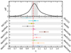 |
Fig. A.1. Upper panel: Probability density function (pdf) of the systematic offset parameter, η, in our cluster sample. The gray band ranges between the 16th and 84th percentile of η in the entire sample. Bottom panel: Median η of each cluster (as indicated in the vertical axes) according to the αturb ≥ 0 model, with error bars corresponding to the 16th and 84th percentiles. For reference, η = 1 (no offset) is indicated with a red vertical line. |
Appendix B: Set-up of the Markov chain Monte Carlo method
Using the emcee13 sampler (Foreman-Mackey et al. 2013), we ran the Markov chain and drew the samples of the parameter vector for each cluster model from the posterior 𝒫. Empirically, we noticed that a combination of Nelson et al. (2013) and Goodman & Weare (2010) moves, as implemented in the emcee sampler, reduces the autocorrelation between successive iterations and optimizes the exploration of the parameter space. We ran the MCMC for 60000 iterations with 500 chains. It is standard to consider the end of the burn-in phase when 𝒫 is found to be stationary as the iteration number increases. The burn-in phase is longer when αturb ≥ 0 than when αturb = 0, but as a rule it lasts less than 5000 steps. In few cases the number of steps of the burn-in phase is higher: ≈15000 for both models of A2319. To be conservative, in all cases we discarded the first 40000 steps. We then applied a thinning of 700 steps to build the posterior sample.
Appendix C: Flattening of the X-ray surface-brightness distributions
Most X-ray surface brightness distributions of the X-COP clusters as resolved in the XMM-Newton maps exhibit clear evidence of a deviation from circular symmetry. Because of the presence of rotation, our models of the X-COP clusters have oblate axisymmetric density distributions, even if the gravitational potential is assumed spherically symmetric. As we assumed that the models are observed edge-on, their surface brightness distributions are flattened. Here we compare the flattening of the models with that observed in the XMM maps.
For the models we evaluated the surface-brightness distribution in each point of the plane of the sky (y, z) as
where ni = n − ne and Λ is the cooling function, which we assume to be independent of temperature (and then of position), as appropriate when considering the soft X-ray band typically used for imaging. We limited ourselves to the region in the plane of the sky, defined by 1 kpc  and 1 kpc
  , where
  is the outer radius of the Nbins,X-th radial bin in the plane of the sky (see Sect. 2.1).
Following B24 (see their Sect. 4.2), we use as measure the flattening of the X-ray 2D surface brightness distribution the axial ratio of isophotes, ζ, computed from the eigenvalues of the 2 × 2 matrix containing the centroids in y, z and yz weighted over the surface brightness. For each cluster model, we randomly extracted 100 parameter vectors from the posterior sample and computed ζ for each parameter vector.
In the upper panel of Fig. C.1, we compare the distribution of ζ in our models to those directly measured in the real clusters. The ζ distribution of the αturb = 0 models (with median 0.91) is more similar to the observed distribution of ζ (with median 0.90) than that of the αturb ≥ 0 models (with median 0.97). However, we note in the αturb = 0 distribution a non-negligible tail at ζ < 0.75 with no counterpart in the observed distribution. The lower panel of Fig. C.1, where we compare the ζ measurements in the models individually with the observed ζ of each cluster, shows that the models of A1795 and A2319 perform better when αturb ≥ 0 than when αturb = 0, while for the other clusters the intervals between the 16th and 84th percentiles in the two models have substantial overlap. In A644 and A2142, neither the αturb = 0 nor αturb ≥ 0 models reproduce the observed ζ at the 1σ confidence level. This might indicate that, in addition to the rotation of the ICM, other properties not accounted for by our models, such as deviations from spherical symmetry of the gravitational potential, non-negligibly contribute to the observed flattenings.
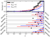 |
Fig. C.1. Observed and model axial ratio, ζ, of the X-ray surface-brightness distributions of the clusters of our sample. Upper panel: Observed distribution of ζ (black) compared to the distributions of ζ of the αturb = 0 (red) and αturb ≥ 0 (blue) models. Lower panel: Observed (squares) ζ compared with the median values of ζ obtained for each cluster (as indicated in the vertical axis) for the αturb = 0 (circles) and αturb ≥ 0 (triangles) models. The error bars indicate the 16th and 84th percentiles measured in our models. The observed data points have very small 1σ uncertainties (δζ/ζ ∼ 10−3), which are not shown in the plot. |
Appendix D: Geometrical approximations in the model-data comparison
Let us consider a generic quantity Q(R, z) that depends on the intrinsic properties of the ICM in an axisymmetric cluster model represented in cylindrical coordinates (R, ϕ, z). In addition to the cylindrical coordinate system, we adopt also a Cartesian system with the same z axis, and with x and y related to R and ϕ by  and ϕ = arctan(x/y). Taking x parallel to the line of sight, we also define a system of polar coordinates in the plane of the sky
  , related to y and z by
  and
and  . For comparison with the observations we need to evaluate integrals of Q over a cylindrical shell with symmetry axis along the line of sight x, and with inner and outer radii
  and
and  , respectively:
where  . We also need to evaluate integrals over spherical shells with inner and outer radii rj and rj + 1, respectively:
Given that our models are neither spherically symmetric nor circularly symmetric in the plane of the sky, the numerical calculation of Eqs. (D.1) and (D.2) is computationally expensive and would represent the bottleneck of our MCMC algorithm. We thus chose to replace Eqs. (D.1) and (D.2) with less time-consuming approximations.
We limited the evaluation of Q to z = 0 plane. Assuming  and Q(R, z)≈Q(R, 0), Eqs. (D.1) and (D.2) become
and
respectively.
All Tables
Lower and upper bounds of the uniform prior distributions of the MCMC parameters γ′IN, γ′OUT, ν⋆, T⋆, Rbreak, log ϵN, log ϵT, upeak, Rpeak, η, and log ϵSZ (common to models both with and without turbulence), and of the parameters log ξ, αinf, and α0 (used only in the model with turbulence).
All Figures
|
Fig. 1. Equatorial plane velocity profiles of the ICM in the αturb = 0 models of the clusters of our sample. Left panel: Ratio between the gas rotation velocity and velocity dispersion (measured in the equatorial plane) as a function of the cylindrical radius normalized to the virial radius, r200 = 3M200/[800πρcrit]1/3, computed using the median value of M200 for each cluster. Right panel: Gas rotation velocity as a function of the cylindrical radius in physical units. In both panels the dashed lines are the median profiles of the individual clusters (as indicated in the legend), whereas the gray band represents the interval between the 16th and 84th percentiles of the distribution of the profiles of the entire sample of clusters. |
| In the text | |
|
Fig. 2. Equatorial plane rotation and turbulence profiles of the ICM in the αturb ≠ 0 models of the clusters of our sample. Upper panels: Same as Fig. 1 but for models with αturb ≥ 0. Lower left panel: Median turbulent-to-total pressure ratio, αturb, as a function of the cylindrical radius normalized to the virial radius, r200 (see the caption of Fig. 1), for the same models as in the upper panels. Lower right panel: 1D turbulent velocity dispersion as a function of the cylindrical radius in physical units for the same models as in the upper panels. The color coding and the meaning of the gray bands are the same as in Fig. 1. In the lower right panel, we overplot the αturb profile measured in simulations by A20 (solid black line; the profile was taken from their Eq. (11), with a0, a1, and a2 equal to their best-fit values, as reported in the first row of their Table 1, and assuming r200, m/r200 ≈ 1.67). |
| In the text | |
|
Fig. 3. Simulated spectrum (black crosses), with an exposure of 100 ks, in half of the Resolve FoV with the best-fit bapec model overplotted. The thermal model only is shown with the green line, the instrumental background in blue, and the thermal model plus the instrumental and cosmic background in red. The most prominent lines are the Fe XXV and Fe XXVI complexes in the range 6−7 keV. |
| In the text | |
|
Fig. A.1. Upper panel: Probability density function (pdf) of the systematic offset parameter, η, in our cluster sample. The gray band ranges between the 16th and 84th percentile of η in the entire sample. Bottom panel: Median η of each cluster (as indicated in the vertical axes) according to the αturb ≥ 0 model, with error bars corresponding to the 16th and 84th percentiles. For reference, η = 1 (no offset) is indicated with a red vertical line. |
| In the text | |
|
Fig. C.1. Observed and model axial ratio, ζ, of the X-ray surface-brightness distributions of the clusters of our sample. Upper panel: Observed distribution of ζ (black) compared to the distributions of ζ of the αturb = 0 (red) and αturb ≥ 0 (blue) models. Lower panel: Observed (squares) ζ compared with the median values of ζ obtained for each cluster (as indicated in the vertical axis) for the αturb = 0 (circles) and αturb ≥ 0 (triangles) models. The error bars indicate the 16th and 84th percentiles measured in our models. The observed data points have very small 1σ uncertainties (δζ/ζ ∼ 10−3), which are not shown in the plot. |
| In the text | |
Current usage metrics show cumulative count of Article Views (full-text article views including HTML views, PDF and ePub downloads, according to the available data) and Abstracts Views on Vision4Press platform.
Data correspond to usage on the plateform after 2015. The current usage metrics is available 48-96 hours after online publication and is updated daily on week days.
Initial download of the metrics may take a while.