


| Issue |
A&A
Volume 709, May 2026
|
|
|---|---|---|
| Article Number | A275 | |
| Number of page(s) | 21 | |
| Section | Stellar atmospheres | |
| DOI | https://doi.org/10.1051/0004-6361/202557865 | |
| Published online | 27 May 2026 | |
The average X-ray spectrum of the volume-complete M-, F-, G-, and K-type star sample within 10 pc of the Sun
1
Max-Planck-Institut für extraterrestrische Physik,
Gießenbachstraße 1,
85748
Garching bei München,
Germany
2
INAF – Osservatorio Astronomico di Brera,
Via E. Bianchi 46,
23807
Merate (LC),
Italy
3
Como Lake centre for AstroPhysics (CLAP), DiSAT, Università dell’Insubria,
via Valleggio 11,
22100
Como,
Italy
4
Institut für Astronomie und Astrophysik, Eberhard Karls Universität Tübingen,
Sand 1,
72076
Tübingen,
Germany
5
Dr. Karl Remeis Observatory, Erlangen Centre for Astroparticle Physics,
Friedrich-Alexander-Universität Erlangen-Nürnberg Sternwartstraße 7,
96049
Bamberg,
Germany
6
Hamburger Sternwarte,
Gojenbergsweg 112,
21029
Hamburg,
Germany
7
Department of Astronomy, University of Science and Technology of China,
Hefei
230026,
China
8
School of Astronomy and Space Science, University of Science and Technology of China,
Hefei
230026,
China
9
Max-Planck-Institut für Radioastronomie,
Auf dem Hügel 69,
53121
Bonn,
Germany
10
Max-Planck-Institut für Astrophysik,
Karl-Schwarzschild-Straße 1,
85748
Garching,
Germany
★ Corresponding author: This email address is being protected from spambots. You need JavaScript enabled to view it.
Received:
28
October
2025
Accepted:
23
February
2026
Abstract
Context. The F-, G-, K-, and M-type stars are the most abundant stellar population in the Milky Way and are expected to contribute to its diffuse X-ray emission. Yet their intrinsic average X-ray spectrum remains poorly constrained due to their faint X-ray luminosities, leaving their collective role in the X-ray background of the Milky Way uncertain.
Aims. We aim to derive a distance-normalised average X-ray spectrum for nearby M dwarfs and F, G, and K stars and to characterise their ensemble spectral properties.
Methods. We analysed the volume-complete sample of M dwarfs (M0-M6) and F, G, and K stars within 10 pc of the Sun using data from the eROSITA all-sky survey aboard the Spectrum-Roentgen-Gamma (SRG) mission (eRASS:4). Individual spectra were normalised by exposure and distance and then stacked to produce representative averages. From these spectra, we derived characteristic X-ray luminosities, which are helpful for estimating the contribution of late-type stars to the soft, diffuse X-ray emission of the Galaxy. Results. The distance-normalised emission measures yield an average X-ray luminosity of (2.6 ± 0.1) × 1027 erg/s for M-type stars, and (15 ± 3) × 1027 erg/s for F-, G-, and K-type stars in 0.2-2.0 keV. The 10-pc average spectra could be well described by a sum of three and two thermal models. The fitted temperatures and abundances remain consistent across M-star sub-groups, while early-M stars are, surprisingly, less luminous on average than mid-to-late-M types. These results offer new insights into the collective X-ray properties of nearby stars in the volume-complete context, and provide motivation to further explore the link with the unresolved soft X-ray background of the Galaxy.
Key words: stars: coronae / stars: late-type / stars: low-mass / X-rays: stars
© The Authors 2026
 Open Access article, published by EDP Sciences, under the terms of the Creative Commons Attribution License (https://creativecommons.org/licenses/by/4.0), which permits unrestricted use, distribution, and reproduction in any medium, provided the original work is properly cited.
This article is published in open access under the Subscribe to Open model.
Open Access funding provided by Max Planck Society.
1 Introduction
Late-type main-sequence stars, such as F-, G-, K-, and M-type stars, are the most numerous stellar type in the Milky Way. M dwarfs alone account for about 70% of the entire stellar population, yet they contribute only about 35% of the total stellar mass. FGK-type stars, though less common (∼23%), provide a comparable fraction of stellar mass (∼35%) (Reid & Gizis 1997; Bochanski et al. 2010; Golovin et al. 2023; Kirkpatrick et al. 2024). Their X-ray emission arises from magnetically heated coronae, where plasma is confined and energised by magnetic fields generated through convection and rotation (Parker 1993; Güdel 2004). Understanding this emission is crucial, as it serves as a proxy for their dynamo and shapes the environments of surrounding planets. Individually, these stars appear as faint X-ray sources even at close distances, but their sheer numbers suggest that they contribute significantly to the soft X-ray background, including the local hot bubble and Galactic halo (Yeung et al. 2024; Ponti et al., in prep.).
A systematic census of the X-ray emission from nearby late-type stars was first carried out with the ROSAT All-Sky Survey, led by Schmitt & Liefke (2004) who compiled the ROSAT/NEXXUS catalogue of all stars in the solar neighbourhood. Deeper observations involving XMM-Newton and Chandra, combined with ROSAT, have since enabled detailed spectral investigations of individual stars. Multi-temperature collisionally ionized thermal model has provided good fits to these stellar coronae, such as in AD Leonis, EV Lac, and EQ Pegasi (Raymond & Smith 1977; Mewe 1991; Robrade & Schmitt 2005).
More recent efforts have been directed towards fully characterising the X-ray properties of volume-limited samples through systematic surveys with the help of Gaia. Based on the Gaia 10-pc catalogue (Reylé et al. 2021), Caramazza et al. (2023) conducted the census of X-ray observations of M dwarfs within the closest 10 pc using ROSAT, XMM-Newton, and eROSITA, probing the faintest levels of coronal emission. Zhu & Preibisch (2025) and Locatelli et al. (2025) also combined the archival X-ray data to study the distribution of luminosity of nearby stars of F to M type in different volumes. Together, these studies provide important constraints on the prevalence and distribution of stellar X-ray activity, with an emphasis on individual luminosity measurements and their relation to other stellar properties.
In this work, we built on these efforts by deriving a distance-normalised stacked X-ray spectrum from the complete, volumelimited sample of nearby late-type stars using data from the four sky surveys of eROSITA (eRASS:4; see Section 3). Our stellar sample is based on the Gaia 10-pc catalogue (Reylé et al. 2021), with the M-dwarf sub-sample (M0-M4) and their coordinates provided by Caramazza et al. (2023), and the complementary M4-M6 and FGK-dwarf lists supplied by Stelzer (priv. comm.). We extracted spectra from the merged eROSITA eRASS:4 event files and stacked them to yield an emissivity-weighted average luminosity for M stars and FGK stars separately.
The paper is structured as follows. The data-selection procedure is described in Section 2; Section 3 presents the data processing; Section 4 explains the stacking approach; Section 6 introduces model fitting and spectral analysis for the averaged spectrum of M0-M6 stars within 10 pc; Section 7 discusses the spectral analysis of FGK-type stars within 10 pc; and finally, Section 9 summarises the results.
2 Sample selection
As mentioned above, we used the volume-complete Gaia-based catalogue of stars within 10 pc of the Sun (Reylé et al. 2021) as the master sample. From this, we adopted the F, G, K, and M0-M6 spectral type (SpT) sub-sample defined by Stelzer et al.(in prep.), which, following Caramazza et al. (2023), assigned a SpT based on Gaia eDR3 GBP - GRP colours using the conversion table compiled by E. Mamajek1. We then restricted the selection to stars located in the western Galactic hemisphere (l ≥ 180°, hereafter WGH), which is accessible to the SRG/eROSITA_DE collaboration.
2.1 Sample overview
Table 1 summarises the number of stars for the sample selection. In total, the 10-pc Gaia catalogue contains 225 M0-M6-type stars and 57 FGK-type stars, of which 109 are M stars, and 32 FGK stars are located in the WGH.
We removed four M stars (IDs 35, 45, 51, and 208; index from Table H.1) and two FGK stars (ID 0 and ID 43; index from Table H.2) due to close proximity to other SpT X-ray sources (‘crowded field’ sources in Table 1). In addition, two M stars (ID 137, 157) were excluded from the final sample due to optical loading. We mark pairs of the same SpT stars separated by less than 5″ as ‘close pairs’ and extracted a single spectrum from a common region encompassing both sources to avoid duplication (see Appendix C for details on the spectral extraction). Eventually, 103 M stars remained after excluding the two stars affected by optical loading (see also Appendix A), constituting the final M-dwarf sample used in this work. We did not exclude FGK stars affected by optical loading (22 of the 32), as excluding them would have severely reduced the completeness of the sample. The final FGK sample to be stacked still comprises 30 stars. In Sect. 2.2 and Appendix A, we compare these 22 optically bright FGK stars’ X-ray fluxes with those of the nine optically faint FGK stars and discuss how the impact of optical loading depends on optical brightness.
In Figure 1, we present the eRASS1-detected (Merloni et al. 2024) M-type and F-, G-, and K-type stars that are used in our sample, showing X-ray luminosity versus Gaia colour (left panel) and total observed counts versus distance for all stars, regardless of whether they were detected in eRASS1 (right panel). Five FGK stars, α Cen A, α Cen B, Procyon A, and HD 156384 A and B, are not shown in Figure 1 as they lack Gaia measurements due to brightness saturation (Reylé et al. (2021). The sample used in this paper has a wider SpT range for M stars (M0-M6) compared to that of Caramazza et al. (2023), which measured the X-ray luminosity of all the detected M0-M4 stars within 10 pc in both the eastern and western hemispheres. According to the luminosity distribution, M stars (M0-M4) in the eastern Galactic hemisphere (EGH) appear to host more high-luminosity sources than the western Galactic hemisphere (WGH). Several of the most luminous M stars, such as AU Mic, AT Mic A, and GJ 867 A and B, are in fact located in the EGH. On average, M stars in the EGH are about 4.7 times more luminous than those in the WGH. For FGK stars (Stelzer, in prep.), the average luminosity in the WGH is slightly higher than in the EGH, i.e. by a factor of about 1.3. Therefore, if one estimates the average luminosity from the EGH, the result can be larger than the one we obtain in this work as our data are limited to the WGH. In Appendix H, we provide the identifiers, coordinates, distances, spectral types, the eRASS1 detection flag (Merloni et al. 2024), and the selection flag of the individual stars used in this work.
Sample selection in this work based on Gaia 10-pc M-type and F-, G-, and K-type stars (Stelzer, priv. comm.).
2.2 Optical loading
In X-ray astronomy, optical loading refers to the interference caused by non-X-ray radiation, such as optical or ultraviolet light, on X-ray detectors (Lumb 2000). While these detectors are primarily designed to detect X-rays, they can also exhibit sensitivity to other types of radiation, which can introduce noise and false signals, particularly in the soft X-ray regime (Ramstedt et al. 2012; Ishikawa et al. 2019). Optical loading can artificially enhance the soft X-ray signal and potentially shift the measured energy of events across the entire spectrum.
To mitigate this effect, we adopted the FLAG_OPT indicator from the eRASS1 catalogue (Merloni et al. 2024), which flags sources potentially affected by optical loading. A source is assigned FLAG_OPT = 1 if it is located within 15″ of a bright optical star (including the source itself) that meets any of the following brightness thresholds: B, V, or G < 4.5 mag, or J < 3 mag. However, the optical-loading threshold also depends on the survey depth; while G<4.5 mag was used for eRASS1, a threshold of G<5.0 mag is more appropriate for eRASS:4 (J. Robrade, priv. comm.).
In Figure 2, we can see no M stars in our sample suffering from optical loading (G < 5), in contrast to more than half of the FGK stars. This result was expected, as the FGK stars are stronger optical emitters than M-dwarf stars. However, as noted earlier, two M-dwarf stars were excluded due to optical loading: GJ 166 C based on its FLAG_OPT indicator; and GJ 442 B, which is part of a visual binary with a separation of 22″ from the bright G-type primary star (GJ 442 A) affected by optical loading.
A detailed explanation of this effect, based on current knowledge of SRG/eROSITA and supported by spectral analysis, is provided in Appendix A. Figure A.2 compares M dwarfs and FGK dwarfs with different G-band magnitudes, showing that M stars’ spectra are consistent and confirming that optical loading has a negligible impact on the M-dwarf sample. In contrast, for FGK stars, a similar test reveals differences on both luminosity and spectral shape, which could originate from optical-loading effects (and the intrinsic luminosity scatter for this limited sample). In Figures A.1a–A.1d, we show three selected FGK stars (G < 5) as examples to examine the possible impact of optical loading by comparing photon-event pattern selections (single, s) with the combined double+triple+quadruple selection (dtq). To obtain a representative average luminosity, we retained all FGK stars but truncated the soft-energy range (<0.35 keV) in this study.
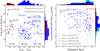 |
Fig. 1 Left: X-ray luminosity (0.1-2.4 keV) versus Gaia GBP-GRP colour for the eRASS1-detected M- and FGK-type stars (Merloni et al. 2024) in the western Galactic hemisphere of the 10-pc Gaia sample. Filled blue circles: eRASS1-detected M dwarfs (l ≥ 180°); filled red circles: eRASS1-detected FGK stars (l ≥ 180°). Notable sources are labeled. Right: eRASS:4 total observed counts in 0.2-2.0 keV versus the distance from the Sun for the 10-pc Gaia sample in the western Galactic hemisphere, with detections and non-detections for M dwarfs (blue, cyan) and FGK stars (brown, coral). |
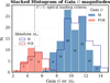 |
Fig. 2 Histogram of Gaia G apparent (G, filled bars) and absolute (MG, outlined bars) magnitudes of the M-type (blue) and FGK-type (red) stars used in this study. The G mag and parallax were taken from Reylé et al. (2021). Five stars with Gaia- saturated magnitudes are not shown here. The vertical dashed line marks the optical loading threshold adopted in this work (G > 5; Robrade, priv. comm.). |
3 Data processing
The eROSITA survey detected most of the late-type stars in the 10-pc Gaia sample (about 75% in eRASS1; Merloni et al. 2024; and over 90% in eRASS:4, in prep.) and scanned all its stars four times over two years, from 2019 December 11 to 2021 December 19. The eROSITA/eRASS:4 data were processed using the standard eROSITA Science Analysis Software System (eSASS), version eSASSusers_240410, developed by the German eROSITA consortium (Brunner et al. 2022). For this study, we used event files from five telescope modules (TMs) with on-chip filters (TM1,2,3,4,6), the combination of which is referred to as TM8. Two modules (TM5 and TM7) lack on-chip optical filters and suffer from light leaks (Predehl et al. 2021), so they were excluded from this study. Using the eSASS task evtool, event files from all four eRASS surveys were combined to create a single event set. All the spectra were collected with all valid patterns (PAT15) when not explicitly mentioned.
4 Method: Spectral stacking
To stack the spectra of stars in the sample, the extraction region for each source was first adjusted to account for proper motion, aligning all positions to a standard reference epoch, 2020 December 15 (Merloni et al. 2012). A single spectrum was generated for each star by merging data from all four eRASS observations (see Appendix C for further details on the extraction procedure). In cases where two stars fell too close together (within 25″), only one combined spectrum was extracted, and both the source and background fluxes were scaled by a factor of two. Each resulting spectrum was then normalized to a reference distance of 10 pc using a scaling factor of (di/10 pc)2, where di is the distance to the star. The background subtraction was performed locally for each source.
Below, we present the full equation used to compute the average rates along with the associated uncertainty:
![Mathematical equation: C_{\text{net,total}} &= \sum_{i=1}^{N} \left[ \left(C_{\text{src},i} - C_{\text{bkg},i} \cdot S_i \right) \left( \frac{d_i}{10\,\text{pc}} \right)^2 \right]\label{eq:AC_C} ,\\](/articles/aa/full_html/2026/05/aa57865-25/aa57865-25-eq1.png) (1)
(1)
 (2)
(2)
 (3)
(3)
Csrc,i and Cbkg,i denote the counts of source region and background from the i-th star, < R > is the averaged count rate of the i-th star, di is its distance in pc, Ti is the exposure time processed by srctool, N is the total number of stars in the sample, and Si is the scaling factor between a source region and background region. The uncertainties in the stacked spectrum, < ER>, reflect the combined Gaussian errors propagated from the individual source spectra. Depending on the definition of stacking, there are multiple ways to combine spectra. The approach described in Eq. (2), which we refer to as the ‘averaging count’ (AC) method, is what we mainly used in this work. Since individual rate varies, the average rate can be more strongly influenced by stars with longer exposures. While approximately 90% of the stars have similar exposure times (processed by srctool) within one standard deviation, a few sources located near the ecliptic pole have significantly longer exposures and therefore might receive much higher weights. To ensure that these high-weight sources do not bias the average spectrum, we also performed additional stacking without them. A comparison of the results with and without these stars is presented in Appendix B.
Alternatively, we could apply the ‘averaging rate’ (AR) method for spectral stacking (Eqs. (4)-(6)). Instead of summing total counts and dividing by total exposure time, this approach computes the average of the count rates across individual sources for each energy channel. Specifically, for each star, the count rate is distance-corrected and then averaged over all sources. The method is mathematically expressed as
 (4)
(4)
 (5)
(5)
 (6)
(6)
where the denotation is the same as Eqs. (1)-(3). This approach normalises counts by exposure before averaging, which ensures each source contributes according to its count rate. However, because standard error propagation assumes statistical independence, it can lead to overestimated uncertainties when stacking spectra with correlated measurements or shared systematics. To mitigate this, we adopted a Gaussian noise assumption, which provides a lower bound on the uncertainties, acknowledging that this likely underestimates the actual statistical error. In Appendix B, we compare the resulting fits and luminosities from this method with those obtained using the AC approach. The differences between them are treated as a source of systematic uncertainty in the final luminosity estimates.
In Appendix B, we compare the best-fit parameters and luminosities obtained from the AC and AR methods, as well as when excluding highly exposed sources, confirming that the stacking procedure does not significantly affect the overall spectral shape.
Given that the effective area of the detector varies with vignetting and masking in the source region, an averaged effective area was computed in each PI channel. While this method is not theoretically optimal, it provides a practical and reproducible approach. Figure 3 presents a statistical comparison of the effective area of TM8 for the sample of 103 M stars and 30 FGK stars. The box plot displays the distribution of the mean effective area. In each box, the solid horizontal line represents the mean value of the sample, while the dashed line indicates the median value. Variations in the effective area amongst sources were mainly caused by masking nearby point sources, with the maximum discrepancies reaching approximately 10% for both samples, as illustrated in the box plot.
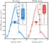 |
Fig. 3 Comparison of effective area of TM8. The box plot represents the statistical distribution of the mean effective area over the 0.2-2.0 keV range. The solid horizontal lines within each box indicate the average value, while the dashed horizontal line (in the zoomed-in plot) represents the median. The sample includes all 103 M stars and 30 FGK stars used in this study. |
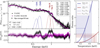 |
Fig. 4 Left panel: averaged 10-pc M-dwarf spectrum with different models. All the models are labelled in the legend, where names follow the XSPEC convention, and the letter G stands for the Gaussian components used to fit single emission lines (dotted lines). Right panel: temperature versus line ratio assuming a single thermal component. The dark red and navy lines show the expected O VIII/OVII and NeX/NeIX ratios from AtomDB. Vertical dashed and dotted lines mark ratios derived from Gaussian normalisations in Table 2. |
5 Analysis: Spectral fitting
The spectral fitting was performed using the pyXspec software (Arnaud 1996). The fitting process assumed elemental abundances from Asplund et al. (2009) and photoelectric absorption cross-sections from Verner et al. (1996). χ2 minimisation was used for the fitting.
Our analysis assumed that the emitting plasma is in collisional ionisation equilibrium (CIE) (Raymond & Smith 1977; Güdel 2004). The analysis begins with a single-temperature, collisionally ionised plasma model, i.e. Astrophysical Plasma Emission Code model (APEC and VAPEC; Smith et al. 2001), which describes a collisionally ionised plasma in stellar coronae of thermal equilibrium. It then progresses towards more complex models, including multi-temperature (2T-APEC and 3T-APEC) (Smith et al. 2001) and variable abundance models (1T-VAPEC, 2T-VAPEC, and 3T-VAPEC). The elemental abundances are tied across all thermal components.
We denote the overall metallicity by Z and the abundance of a specific element by AX. The metal abundance (AX) is defined as  . With the VAPEC model, we allowed O, Ne, Si, and Fe to vary independently; all other elements (He, C, N, Mg, Al, S, Ar, Ca, Ni) were tied together and allowed to vary as a single free parameter. Alpha elements such as oxygen, neon, and silicon were primarily considered (Bensby et al. 2014; Jofré et al. 2015; Montes et al. 2018). We verified that we could not obtain improvement in the fit by untying any of the abundances of the other elements. More parameter initializations are listed in Appendix D.
To assess the relative quality of spectral fits, we employed the Fisher test (F-test), the Bayesian information criterion (BIC; Schwarz 1978), and the Akaike information criterion (AIC; Akaike 1974). The F-test evaluates whether the addition of extra parameters significantly improves the fit, assuming nested models and Gaussian errors. The AIC and BIC are both informationtheoretic criteria that balance model goodness of fit against complexity, with the BIC applying a penalty for the complex models. In our case, we adopted AIC=2k +  and BIC=k ln(N) +
  , where k is the number of free parameters and N is the number of data channels.
6 Results: M-dwarf sample
In this section, we describe how we fitted the average X-ray spectrum of M dwarfs. Unless stated otherwise, the M-star spectra were fitted within the energy range of 0.2-2.0keV, where the signal-to-noise ratio (S/N) of the stacked spectra, which is scaled to 10 pc, exceeds one.
The results of the fitting procedure for the sequence of models are summarized in Table 2, while the corresponding multi-temperature spectral fits are presented in Figure 5. The uncertainties correspond to 90% confidence intervals for a single parameter assuming chi-squared statistics. The bootstrap uncertainties (90% CI) are reported as the second term in the brackets of the corresponding parameter. The F tests between models are provided in Table 3.
Model parameters and values for M-dwarf averaged spectrum.
6.1 Single-temperature plasma models
The single temperature APEC model yielded a poor fit ( = 2.12) with kT = 0.66 ± 0.02 keV and an unusually low abundance of Zall = 0.061 ± 0.006 Z⊙, which is lower than the typical values found in stellar coronae: Z ≈ 0.3-0.4 Z⊙ (e.g. Favata et al. 2004, and Robrade & Schmitt 2005).
This is likely a spectral modelling bias related to stacking, similar to the ‘artificial Fe bias’ reported in studies of galaxy group and cluster, where a multi-temperature plasma (with different thermal components) was modelled using a singletemperature APEC model (Buote 2000; Sanders & Fabian 2011).
Residuals at 0.5-0.7 keV and 0.9-1.1 keV align with known strong emission lines, such as O VII, O VIII, Ne IX, and Ne X. This is demonstrated by the improved fit obtained by adding four Gaussian components at energies close to those of the brightest emission lines. In addition, treating the normalizations of the added Gaussian components as line intensities, we derived the O VIII/O VII ratio (blue dotted lines) and Ne X/Ne IX (red dotted lines). Those ratios, however, were inconsistent with theoretical ratios expected from a single temperature plasma, as shown in the right panel of Figure 4. This hinted at the need for an additional temperature component.
6.2 Multi-temperature plasma models
A dual-temperature APEC model (2T-APEC:  = 0.93) provided a significant improvement over the single-temperature APEC model and performed better than the single VAPEC model, as indicated by the F-test (see Table 3) and the AIC and BIC criteria. This suggests that the improvement in the fit is primarily driven by the inclusion of a second thermal component rather than by adjustments to the elemental abundances. The two plasma temperatures are kT1 = 0.27 ± 0.01 keV and kT2 = 0.94 ± 0.03 keV, with a tied abundance of Zall = 0.28 ± 0.04. Though it is a relatively good fit, the residuals in the upper left panel of Figure 5 show the presence of a significant excess below 0.3 keV and a bump near 1.9 keV.
Adding a third temperature component (3T-APEC:  = 0.91) further improved the fit (see F test in Table 3; see AIC and BIC in Table 2). The additional cooler component has a poorly constrained temperature and normalization: kT1 = 0.1 ± 0.1 keV and N1 =
  . From the upper left panel in Figure 5, we can see this component contributes only a tiny range of energies to the spectrum (<0.3 keV), effectively coming up (only) for the low-energy excess seen in the 2T-APEC model. In fact, the fitted temperatures of the second and third components are consistent with those obtained in the 2T-APEC model. Adding this component yields only a modest improvement, and the F test does not support it as statistically significant (p value=0.024).
We further applied 2T- and 3T-VAPEC models, with the elemental abundances linked between the two or three components. As mentioned in Sect. 5, the abundances of elements O, Ne, Si, and Fe were allowed to vary freely, while all other elements were tied together to vary. According to the statistical estimators, the 2T-VAPEC model ( = 0.92) provided a comparably good fit to that of the 2T-APEC model, but it requires four additional free parameters, making it the less favoured choice.
The 3T-VAPEC model ( = 0.84) appeared mildly overfitted, requiring an additional third component at a very soft temperature of 0.09 ± 0.09 keV, which is not constrained at all. Varying the elemental abundances alone does not resolve the soft excess and only shuffles the relative strength of the elements or components of the fit (see Appendix D).
This poorly constrained, very soft component is atypical for M stars and may instead reflect calibration uncertainties at the lowest energies. After updating to the most recent response files, calibrated using soft neutron-star spectra, its significance is already reduced compared to the previous version. We therefore restricted the subsequent analysis to two-temperature models and adopted the 2T-APEC model as our baseline. This model provides a simple description while retaining the key feature that its two components at 0.27 keV and 0.96 keV are also consistently required in the 2T-VAPEC and 3T-APEC models. We used the 2T-APEC model as the best fit for the following sub-group analysis of the M-star sample.
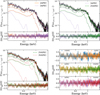 |
Fig. 5 Model fitting of the averaged X-ray spectra (0.2-2.0 keV) of 103 M-dwarf stars using multi-temperature thermal plasma models. The top left, top right and bottom left panels show comparisons between two-temperature and three-temperature APEC models (labelled as 2APEC and 3T-APEC), and as variable-abundance counterparts (2T-VAPEC and 3T-VAPEC). The corresponding residuals are shown. The bottom right panel presents a comparative view of residuals amongst four models to assess the fit quality. |
6.3 Luminous M dwarfs versus the remaining sample
The X-ray-luminous stars potentially skew the spectral characteristics from the average spectral shape. In this section, we examined how AD Leonis and other very luminous stars affect the features of stacked average spectra. As shown in the left panel of Figure 1, AD Leo (AD Leo or BD+20 2465) stands out as the most luminous in our sample, lying near the upper envelope of the luminosity distribution. Although its colour corresponds to an early-M type (M3.5V), its X-ray luminosity is nearly an order of magnitude higher than that of typical M0-M4 stars, which is consistent with its well-known status as a magnetically active flare star (Stelzer et al. 2022). Following AD Leo are YZ CMi and G 41-14 AB, which are themselves about two times more luminous than AP Col. We therefore defined these four brightest M stars as the M4L group. Hence, we define two groups of stars: AD Leo to the remaining 102 M dwarfs with lower luminosity (M102R), and the four most luminous M stars (M4L) with the remaining 99 less luminous M stars (M99R).
Figure 6a shows the average X-ray spectra of the four groups, with the best-fit models from Table 4 overlaid. The 2T-APEC model was applied to the data over 0.2-2.5 keV, a broader range than in the other analysis of this work, to examine the harder spectrum that is expected for active stars. The average spectrum of M102R was scaled up by a factor of 30 to match the distance-normalised flux of AD Leo at 0.7 keV, while the M4L spectrum was scaled down by a factor of 20 to align with the flux of M99L at the same energy. From the ratio panel in the bottom of Figure 6a (flux normalised at 0.7 keV), we observed that AD Leo closely resembles M102R in the intermediate energy range (0.3-0.9 keV). The deviations increase at higher energies (>0.9 keV) and AD Leo exhibits overall harder spectrum. A similar trend is seen for M4L when compared with M99R.
The best-fitting parameters are listed in Table 4. The average spectra of M99R, M102R, and M4L are well described by two components with temperatures of ~0.27 and 0.92-1.03 keV, yielding good fits with  < 0.8 that indicate slight over-fitting. The fits for spectra of AD Leo were fitted with components at 0.26, 0.94, and 1.5 keV. The fitting of AD Leo is marginally acceptable:
  = 1.3. The residuals scatter at 0.45-0.6 keV.
The M102R, M99R, and M4L samples have remarkably consistent best-fitting parameters (T and Z) in relation to each other and with the whole M-star sample in Table 2. All spectra share a consistent intermediate-temperature component (~0.27 keV) and hotter components at (~0.9 keV). Those two contribute the majority of the emission. Only AD Leo exhibits an additional high-temperature component around 1.5 keV and higher coronal abundances ( ) compared to the rest of the groups. The relatively poor fit of AD Leo may reflect its distinct magnetic activity that is not fully captured at the current energy resolution. Despite its individual peculiarities, both AD Leo’s and M4L’s overall spectral shapes remain broadly similar to those of other M dwarfs in the central energy range. By comparing with the best fit of all M stars in Table 2, we conclude that either excluding AD Leo or the four most luminous stars from the stacked sample, does not significantly alter any parameter except for the overall normalisation.
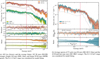 |
Fig. 6 Comparison between X-ray brightness sub-groups and sub-spectral-type groups. All spectra are normalised to a distance of 10 pc and aligned at 0.7 keV for comparison. Each spectrum is fitted with a 2T-APEC model. The residual ( |

F-test statistics of models for average M star.
Fitting parameters for different luminosity groups.
Fitting parameters for average spectra of M0-M3.5 and M4-M6.5 sub-groups.
6.4 Early-type M dwarfs versus late-type M dwarfs
The structural differences between early-type and late-type M dwarfs are particularly relevant for analysing their X-ray spectral properties. Early-type M dwarfs possess a radiative core, whereas mid- and late-type M dwarfs are fully convective. This can influence their X-ray emission characteristics, which may be obscured if the two groups are combined in the analysis.
To investigate this distinction, we divided the 10 pc sample of M dwarfs into M0-M3.5 (early-type) and M4-M6.5 (mid- and late-type) groups. For clarity and to minimise potential biases, we excluded a pair of M stars, CD −37 10765 A (M3V) and B (M5V), which belong to different sub-spectral-type groups and are not distinguishable in X-rays. The final sample comprises 57 stars of sub-type M0-M3.5 and 44 stars of sub-type M4-M6.5, with two stars excluded.
Figure 6b presents the X-ray spectra of the two groups; M0-M3.5 exhibit lower flux than M4-6.5 in the studied energy range; hence, we scaled up the flux of the M0-M3.5 group by a factor of 1.73 to match the flux of the M4-M6.5 group at 0.7 keV for comparison. The top panel shows the fit using the two-temperature 2T-APEC model (see also in Table 5), and the middle panel displays the residuals of the fits. The bottom panel of Figure 6b shows the ratio between the scaled spectrum of the M0-M3.5 group and that of the M4-M6.5 group.
By visual inspection, the spectra reveal overall consistency in spectral shape despite the different luminosities, especially in the 0.5-2.0 keV range from the ratio plot. The mismatch rises in the very soft (<0.5 keV) band as the early-type M dwarfs display a relatively softer flux than the mid- and late-type ones.
Table 5 summarises the spectral fits for M0-M3.5- and M4-M6.5-type M dwarfs using 3T-APEC models. Both fits achieve low reduced χ2. The metal abundances are consistent between the two groups. The temperatures of the intermediate and hot components (kT1 and kT2) are in good agreement between the two groups. Interestingly, the M0-M3.5 stars in our sample are approximately 40% fainter in X-ray luminosity compared to their M4-M6.5 counterparts, contrary to conventional expectations. Early-type M dwarfs, in which a radiative core remains beneath their convective envelopes, are generally thought to sustain higher coronal temperatures and produce more energetic flares, leading to stronger X-ray emission, particularly at harder energies. Late-type M dwarfs, on the other hand, are fully convective and often exhibit saturated magnetic activity. While this can maintain a high X-ray luminosity relative to their bolometric output, they are not usually expected to surpass earlier types in absolute luminosity due to LX - M* dependence (see e.g. Magaudda et al. 2022; Magaudda et al. 2020). The observed trend suggests that additional effects, such as sample selection biases or flare activity, may contribute to the emission. It would therefore be valuable to test the luminosity-spectral-type relation with larger samples and assess whether the 10-pc stars are systematically different from the common Galactic population.
7 Results: F-, G-, and K-type star sample
In this section, we describe how we applied the same spectral fitting approach used for the M dwarfs to the stacked spectra of FGK-type stars within the 10-pc WGH sample. The spectrum shown in Figure 7 is constructed from 30 FGK-type dwarf stars, all included in the eROSITA_DE sky survey. While this dataset comprehensively measures nearby FGK-type stars, the limited sample size may not fully capture the diversity of coronal properties present within this stellar class. FGK dwarfs are brighter than M dwarfs in the optical and ultraviolet bands. A high optical and UV brightness potentially introduces optical loading on the SRG/eROSITA detectors. This effect alters the information on the detected photons (number, energy, and detection pattern) and becomes increasingly important at lower energies. In fact, a significant number of these FGK stars are potentially affected by optical loading. To retain all 30 FGK-type stars in the analysis, we restricted our spectral fitting to energies above 0.35 keV. By doing so, we mitigated the influence of optical loading, whose effect is only significant at lower energies (see Appendix A). We note that this treatment largely helped to reduce the flux excess at the soft end; however, it is important to note that the blueshift caused by optical loading affects the entire energy range. We present spectra affected by and free from optical loading below 0.35 keV in Appendix A, and we tested them with the 3T model.
The parameters obtained from all fitted models are summarised in Table 6. Similarly to the M-dwarf case, the fit using a single-temperature APEC model (1T-APEC) yields statistically unacceptable results, with a reduced chi-squared of  . The same considerations are valid when adding complexity to this simple model. We thus do not discuss this model further. The 1T-VAPEC model, which allows metal abundances to vary, also provides a poor fit with
  . Together with the inadequate fit of the 1T-APEC model, this result suggests that a single-temperature description is insufficient—even when elemental abundances are allowed to vary. Therefore, we added a second APEC model (2T-APEC; top left panel in Figure 7), which significantly improved the fit, reducing the chi-squared by
  for two additional d.o.f. (see Table 6).
The 2T-VAPEC model further improves the fit compared to both the 1T-VAPEC model and the 2T-APEC model in relation to the F test (see Table 7). The best-fit temperatures for the two components are 0.22 ± 0.01 keV and 0.60 ± 0.02 keV, with corresponding abundances of  , and
, and  , and a shared abundance of
  for the rest of the elements.
Instead of leaving the metal abundances free to vary, another way to add complexity with respect to the 2T-APEC model is to introduce a third thermal component (with linked abundance across all components). This 3T-APEC fit ( ) also shows improvement relative to the 2T-APEC model. The F-test comparison, F(2,96.36), also supports the 3T-APEC model over the 2T-APEC configurations. The best-fit temperatures from the 3T-APEC model are kT1 = 0.09 ± 0.01 keV, kT2 = 0.35 ± 0.02 keV, and kT3 = 0.79 ± 0.03 keV, with a shared abundance of
  . The presence of the very soft component (kT1 = 0.09 ± 0.01) could be a residual effect of optical loading.
An F test comparing the 2T-VAPEC and 3T-APEC fits yields (F(2,17.61)=8.1), exceeding the 3σ threshold and favouring 2T-VAPEC over 3T-APEC. This indicates that improving the 2T-APEC description by allowing metal abundances to vary is more effective than adding an extra thermal component. At the same time, while 3T-VAPEC improves upon 3T-APEC, it does not outperform 2T-VAPEC: the comparison between 3T-VAPEC and 2T-VAPEC gives (F(2,5.77)=2.7) (p = 0.069), below 3σ significance. Considering ∆AIC and ∆BIC alongside the F tests, we adopted 2T-VAPEC as the conservative model for the subsequent discussion.
Although this analysis includes all FGK stars within the 10pc WGH, the limited sample size may not provide a sufficiently comprehensive spectroscopic view of the unified properties of local FGK stars. Further studies employing higher resolution spectra and/or larger samples will be essential to refine these preliminary findings, especially regarding the softest end of the energy band considered here.
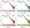 |
Fig. 7 Model fitting of averaged X-ray spectra of 30 FGK stars (0.35-2.0 keV) using multi-temperature thermal plasma models. The four panels compare the performance of two-temperature and three-temperature APEC and VAPEC models, with corresponding residuals shown below each spectrum. The corresponding residuals are shown. |
8 Results: Average luminosities
In Table 8, we report the flux and luminosity in different energy bands for the eROSITA_DE stacked 10 pc (WGH) M-dwarf spectrum based on the 2T-APEC and 2T-VAPEC models. The flux from component 0.27 keV and 0.94 keV is reported in 0.2-2.0 keV and extrapolated for 0.1-2.4 keV, which is the band pass of the ROSAT PSPC. We also derived FGK average luminosities for the 2T-VAPEC and 3T-VAPEC models in Table 9. We define and report conservative uncertainties for flux and luminosity by accounting for the differences between the AC and AR stacking methods. Specifically, the quoted uncertainties were taken as the envelope (union) of the 90% χ2 statistical confidence and intervals and the systematic offset between results produced by the AC and AR methods. This provides a lower bound on the total uncertainty compared to that derived from model fitting.
In the 0.2-2.0 keV band, M dwarfs exhibit an average luminosity of (2.6 ± 0.1) × 1027 erg s−1 (2T-APEC), while FGK stars have (15 ± 3) × 1027 erg s−1 (2T-VAPEC). Thus, the averaged FGK star in 10 pc (WGH) is more than five times brighter than an M dwarf in this energy range. In Figure 8, we present the spectra of M stars and FGK stars overlaid with their respective model fits. By comparing the M-star and FGK-star spectra in the bottom panel of Figure 8, we find the overall similarity, except the primary difference arising in the 0.7-0.9 keV energy range.
In Figure F.1, we also show that there is no significant systematic variation in the average luminosity is observed across the four eRASS epochs.
Independent of the ten-WGH sample considered in this work, early-type M stars (M0-M4) in the EGH appear to host more high-luminosity sources than the WGH. Across the combined WGH+EGH 10-pc Gaia sample, M dwarfs can exhibit a mean luminosity of up to ~6 × 1027 erg s−1, as inferred from Caramazza et al. (2023). By comparison, the FGK sample shows no measurable hemispheric dependence in its average luminosity.
Model parameters and values for F-, G-, and K-dwarf-averaged spectra.
F-test statistics of models for the average FGK star.
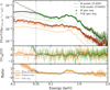 |
Fig. 8 Comparison of spectra of 103 M stars (orange) and 30 FGK stars (green) in the 10-pc Gaia sample. Models 2T-apec and 2T-VAPEC were applied, respectively. The middle panel displays the residual of the fit. The bottom panel shows the ratio between the average FGK and 5.55 times brighter M-star spectra. The scale comes from the ratio of luminosity in 0.2-2.0 keV. The Poisson noise is applied. |
Fluxes and luminosities of stacked M-star spectra.
Fluxes and luminosities of stacked FGK-star spectra.
9 Conclusions
In this study, we produced the highest signal-to-noise distance- normalised spectrum of M dwarfs and FGK-type stars by stacking over the volume-complete sample of stars within 10 pc in the western Galactic hemisphere, using data from the first four X-ray surveys of the sky performed by the SRG/eROSITA instrument (eRASS1 to 4). The average X-ray luminosity of WGH in 0.2-2.0 keV is of (2.6 ± 0.1) × 1027 erg/s for 10 pc M-type stars, and (15 ± 3) × 1027 erg/s for F-, G-, and K-type stars. When considering the entire 10-pc Gaia sample in both WGH and EGH, the average luminosity for the M star sample could be as high as ∼6 × 1027 erg/s, cross-estimated from Caramazza et al. (2023), whereas the average luminosity of FGK stars shows no significant difference between the two hemispheres. The luminosities derived here are in good agreement across all four eRASS surveys. The stacked spectra are well reproduced by collisionally ionised plasma components at different temperatures. The fitted temperature structure and abundances remain consistent despite the presence of the most luminous outliers in the brightness distribution. Specifically, all M-star sub-samples tested exhibit the same two thermal components, at approximately 0.27 keV and 0.94 keV. Additional softer or harder components are required depending on the energy range considered and ongoing flaring activity. Apart from the emission measure, no evidence of systematic differences in the fitted parameters are found between the stacked spectra of early-type (M0-M3.5) and mid-to-late-type (M4-M6.5) M dwarfs. Interestingly, the early M stars appear on average less luminous than the mid- and late-M stars, in contrast to the expected LX-M* trend (Magaudda et al. 2022).
Our study provides insights into nearby low-mass stars’ X-ray luminosity properties. In this work, we used the highest statistics from the four eROSITA All-Sky Surveys combined. Potential improvement may come from the availability of models to account for optical loading.
Data availability
The catalogue is available at the CDS via https://cdsarc.cds.unistra.fr/viz-bin/cat/J/A+A/709/A275
Acknowledgements
This work is based on data from eROSITA, the soft X-ray instrument aboard SRG, a joint Russian-German science mission supported by the Russian Space Agency (Roskosmos), in the interests of the Russian Academy of Sciences represented by its Space Research Institute (IKI), and the Deutsches Zentrum für Luft und Raumfahrt (DLR). The SRG spacecraft was built by Lavochkin Association (NPOL) and its subcontractors, and is operated by NPOL with support from the Max Planck Institute for Extraterrestrial Physics (MPE). The development and construction of the eROSITA X-ray instrument was led by MPE, with contributions from the Dr. Karl Remeis Observatory Bamberg & ECAP (FAU Erlangen-Nuernberg), the University of Hamburg Observatory, the Leibniz Institute for Astrophysics Potsdam (AIP), and the Institute for Astronomy and Astrophysics of the University of Tübingen, with the support of DLR and the Max Planck Society. The Argelander Institute for Astronomy of the University of Bonn and the Ludwig Maximilians Universität Munich also participated in the science preparation for eROSITA. The eROSITA data shown here were processed using the eSASS/NRTA software system developed by the German eROSITA consortium. We acknowledge financial support from the European Research Council (ERC) under the European Union’s Horizon 2020 research and innovation program Hot-Milk (grant agreement No. 865637). GP acknowledges support from Bando per il Finanziamento della Ricerca Fondamentale 2022 dell’Istituto Nazionale di Astrofisica (INAF): GO Large program and from the Framework per l’Attrazione e il Rafforzamento delle Eccellenze (FARE) per la ricerca in Italia (R20L5S39T9). MF and MY acknowledge support from the Deutsche Forschungsgemeinschaft through the grant FR 1691/2-1. W.B. acknowledges support from the Deutsche Forschungsgemeinschaft through the project BE 1649/11-1 and BE 1649/11-2 within the Research Unit FOR 2990 (eRO-STEP).
References
- Akaike, H. 1974, IEEE Trans. Automatic Control, 19, 716 [CrossRef] [Google Scholar]
- Arnaud, K. A. 1996, in Astronomical Society of the Pacific Conference Series, 101, Astronomical Data Analysis Software and Systems V, eds. G. H. Jacoby, & J. Barnes, 17 [Google Scholar]
- Asplund, M., Grevesse, N., Sauval, A. J., & Scott, P. 2009, ARA&A, 47, 4811 [Google Scholar]
- Bensby, T., Feltzing, S., & Oey, M. S. 2014, A&A, 562, A71 [NASA ADS] [CrossRef] [EDP Sciences] [Google Scholar]
- Bochanski, J. J., Hawley, S. L., Covey, K. R., et al. 2010, AJ, 139, 2679 [NASA ADS] [CrossRef] [Google Scholar]
- Brunner, H., Liu, T., Lamer, G., et al. 2022, A&A, 661, A1 [NASA ADS] [CrossRef] [EDP Sciences] [Google Scholar]
- Buote, D. A. 2000, ApJ, 539, 172 [NASA ADS] [CrossRef] [Google Scholar]
- Caramazza, M., Stelzer, B., Magaudda, E., et al. 2023, A&A, 676, A14 [NASA ADS] [CrossRef] [EDP Sciences] [Google Scholar]
- Dennerl, K., Andritschke, R., Bräuninger, H., et al. 2020, SPIE Conf. Ser., 11444, 114444Q [NASA ADS] [Google Scholar]
- Favata, F., Micela, G., Baliunas, S. L., et al. 2004, A&A, 418, L13 [NASA ADS] [CrossRef] [EDP Sciences] [Google Scholar]
- Golovin, A., Reffert, S., Just, A., et al. 2023, A&A, 670, A19 [NASA ADS] [CrossRef] [EDP Sciences] [Google Scholar]
- Güdel, M. 2004, A&A Rev., 12, 71 [Google Scholar]
- Ishikawa, K., Ezoe, Y., Ohashi, T., Kimura, T., & Miyoshi, Y. 2019, Proc. Int. Symp. Planet. Sci., 2011 [Google Scholar]
- Jofré, P., Heiter, U., Soubiran, C., et al. 2015, A&A, 582, A81 [Google Scholar]
- Kirkpatrick, J. D., Marocco, F., Gelino, C. R., et al. 2024, ApJS, 271, 551 [Google Scholar]
- Locatelli, N., Ponti, G., Magaudda, E., & Stelzer, B. 2025, A&A, 702, A2371 [Google Scholar]
- Lumb, D. 2000, PHS Tools - EPIC Optical Loading [Google Scholar]
- Magaudda, E., Stelzer, B., Covey, K. R., et al. 2020, A&A, 638, A20 [NASA ADS] [CrossRef] [EDP Sciences] [Google Scholar]
- Magaudda, E., Stelzer, B., Raetz, S., et al. 2022, A&A, 661, A29 [NASA ADS] [CrossRef] [EDP Sciences] [Google Scholar]
- Meidinger, N., Andritschke, R., Dennerl, K., et al. 2021, J. Astron. Telesc. Instrum. Syst., 7, 025004 [Google Scholar]
- Merloni, A., Predehl, P., Becker, W., et al. 2012, arXiv e-prints [arXiv:1209.3114] [Google Scholar]
- Merloni, A., Lamer, G., Liu, T., et al. 2024, A&A, 682, A34 [NASA ADS] [CrossRef] [EDP Sciences] [Google Scholar]
- Mewe, R. 1991, A&A Rev., 3, 127 [Google Scholar]
- Montes, D., González-Peinado, R., Tabernero, H. M., et al. 2018, MNRAS, 479, 1332 [Google Scholar]
- Neves, V., Bonfils, X., Santos, N. C., et al. 2012, A&A, 538, A25 [NASA ADS] [CrossRef] [EDP Sciences] [Google Scholar]
- Parker, E. N. 1993, ApJ, 408, 707 [NASA ADS] [CrossRef] [Google Scholar]
- Predehl, P., Andritschke, R., Arefiev, V., et al. 2021, A&A, 647, A1 [EDP Sciences] [Google Scholar]
- Ramstedt, S., Montez, R., Kastner, J., & Vlemmings, W. H. T. 2012, A&A, 543, A147 [NASA ADS] [CrossRef] [EDP Sciences] [Google Scholar]
- Raymond, J. C., & Smith, B. W. 1977, ApJS, 35, 419 [NASA ADS] [CrossRef] [Google Scholar]
- Reid, I. N., & Gizis, J. E. 1997, AJ, 113, 2246 [NASA ADS] [CrossRef] [Google Scholar]
- Reylé, C., Jardine, K., Fouqué, P., et al. 2021, A&A, 650, A201 [Google Scholar]
- Robrade, J., & Schmitt, J. H. M. M. 2005, A&A, 435, 1073 [NASA ADS] [CrossRef] [EDP Sciences] [Google Scholar]
- Sanders, J. S., & Fabian, A. C. 2011, MNRAS, 412, L35 [NASA ADS] [CrossRef] [Google Scholar]
- Schmitt, J. H. M. M., & Liefke, C. 2004, A&A, 417, 651 [NASA ADS] [CrossRef] [EDP Sciences] [Google Scholar]
- Schwarz, G. 1978, Ann. Statist., 6, 461 [Google Scholar]
- Smith, R. K., Brickhouse, N. S., Liedahl, D. A., & Raymond, J. C. 2001, ApJ, 556, L91 [Google Scholar]
- Stelzer, B., Caramazza, M., Raetz, S., Argiroffi, C., & Coffaro, M. 2022, A&A, 667, L9 [NASA ADS] [CrossRef] [EDP Sciences] [Google Scholar]
- Verner, D. A., Ferland, G. J., Korista, K. T., & Yakovlev, D. G. 1996, ApJ, 465, 487 [Google Scholar]
- Woolf, V. M., & Wallerstein, G. 2005, MNRAS, 356, 963 [NASA ADS] [CrossRef] [Google Scholar]
- Yeung, M. C. H., Ponti, G., Freyberg, M. J., et al. 2024, A&A, 690, A399 [NASA ADS] [CrossRef] [EDP Sciences] [Google Scholar]
- Zhu, E., & Preibisch, T. 2025, A&A, 694, A93 [NASA ADS] [CrossRef] [EDP Sciences] [Google Scholar]
Appendix A The impact of optical loading on the spectrum of bright stars
When an X-ray photon reaches the depletion layer of an X-ray CCD, it creates electron-hole pairs there (Dennerl et al. 2020; Meidinger et al. 2021). The same may happen when an optical photon reaches this layer. In contrast to an X-ray photon, however, where the number of released electrons can be utilized for spectroscopy, the absorption of a single optical photon releases typically only one electron. This charge alone is not high enough to get included into the telemetry stream, because it is below the low energy threshold, which needs to be applied in order to prevent telemetry overload due to electronic noise. In the case of celestial sources which are both optically and X-ray bright, however, the similar (though not identical) optical and X-ray point-spread function (PSF) favour the case that the charge clouds created by the optical and X-ray photons get superimposed within the integration time of a particular CCD frame. In the following we discuss the consequences of that case.
For better clarity we start with a simplified example, which considers the presence of only one X-ray and one optical photon and assumes absence of electronic noise. In that case, the observed spectrum is modified due to the additional charge generated by the optical photon in two ways:
energy: the spectrum gets ‘blue-shifted’, and because of the Poissonian nature of the additional charge, it gets (somewhat) smeared; while these effects are most apparent at low energies, they affect the whole spectrum.
flux: the geometry and extent of the charge cloud get modified, causing a change of the reconstructed flux.
While the consequences of optical loading on the energy is straightforward, its impact on the flux requires a more detailed investigation. We need to consider that the charge cloud created by an X-ray photon may extend over up to four pixels, which we refer to as ‘singles (s)’, ‘doubles (d)’, ‘triples (t)’, and ‘quadruples (q)’. The triples and quadruples have to meet the following criteria in order to have been generated by an X-ray photon: the triples must be L-shaped, with the main pixel (the one containing the dominant charge component) at the corner, and the quadruples must be quadratic, with the main pixel essentially opposite to the pixel containing the minimum charge. Only such triples and quadruples are considered as ‘valid’ and are used for reconstructing the flux (for the singles and doubles there is no restriction on their validity other than that they must be sufficiently far away from an insensitive area). The additional charge generated by an optical photon can then modify the pixel pattern in several ways:
it neither changes the pattern size nor the validity of the pattern: then only the energy is affected, but not the flux (when taking the energy shift into account); this holds also for the pattern-specific flux, derived, e.g., from considering only singles.
it increases the pattern size, but keeps the pattern valid: then the energy and the pattern-specific flux are affected, but not the ‘sdtq’ flux; the increase of the pattern size is caused by raising the charge in a neighbouring pixel above the low energy threshold.
it makes the pattern invalid: then the X-ray photon gets lost and the flux is reduced, but the energy scale is not affected.
If we consider the presence of several optical photons (optical pile-up), then this situation stays unaffected as long as the optical photon flux is not high enough to generate charge above the low energy threshold without an X-ray photon. However, when this happens, the affected pixels have to be masked out in order to avoid saturation of telemetry. Therefore, this case does not need further consideration. Similarly, the presence of several X-ray photons (X-ray pile-up) as well as the combination of optical and X-ray pile-up does not need to be considered here, because it might prevent a spectroscopic analysis.
What still needs to be considered is the presence of electronic noise, which is steeply rising towards the low energy threshold (which is the reason why such a threshold needs to be applied). Superposition with the charge released by optical photons causes its spectrum to get ‘blue-shifted’ in a similar way as an X-ray spectrum, making it appear amplified and creating the impression of the presence of an additional soft ‘optical’ component. While to some extent this effect is mitigated by considering the local background in the spectral analysis, an apparent soft energy component may remain. For completeness we mention that there is in addition particle induced background present, which may also be affected by optical loading. This component, however, is comparatively faint.
Appendix A.1 Between patterns and TMs
The effects described above can be utilized for studying the eROSITA spectra for evidence of optical loading. In the following we present FGK spectra which are divided by the effective area (indicated by ‘cm−2’) for better clarity as significant number of FGK stars are optically bright, with G-band magnitudes below 5, potentially causing strong optical loading.
Figure A.1a investigates the effect 1 by comparing patternspecific spectra: ‘s’ (black) with ‘dtq’ (red). The fact that ‘s’ is only slightly below ‘dtq’ indicates that the pattern size and validity of the patterns are not much affected, indicating only minor optical loading. In contrast, Figure A.1b presents a case where ‘s’ is considerably below ‘dtq’, which is evidence for substantial optical loading. Subdividing the ‘dtq’ spectrum of Figure A.1b into the individual ‘d’, ‘t’, and ‘q’ components (Figure A.1c) shows that the apparent spectral flux increases with pattern size up to triples. This is consistent with effect 2: if the charge cloud created by the absorption of an X-ray photon is distributed over more pixels, then the probability that an optical photon hits a pixel in that cloud is increased. This, however, does not apply to quadruples, because any extension beyond four pixels makes a pattern invalid, leading to a loss of flux (effect 3). This loss, however, is quite small, because the probability that quadruples are created by an X-ray photon below 0.5 keV is less than 3%.
Another way of checking for optical loading is to compare the spectra between TM8 and TM9, as they differ in the thickness of the Al layer in the optical blocking filter, which is 200 nm for TM8 and 100 nm for TM9 (Meidinger et al. 2021). Thus, TM9 is more sensitive to optical flux than TM8. Figure A.1d shows that for source #13 (the same as in Figure A.1a) the ‘sdtq’ spectra for TM8 and TM9 (when divided by the effective area) are similar. This indicates that the derived luminosity is not much affected by optical loading (effect 2), consistent with the conclusion above, which was based on a comparison between the ‘s’ and ‘dtq’ spectra forTM8 (effect 1, Figure A.1a). For source#34 (Figure A.1e), however, TM9 is clearly below TM8, and for source #38 (Figure A.1f), TM9 is considerably below TM8 a clear indication for optical loading. Source #13, #34 and #38 are eps Eri (K2V star with G3.5 mag), π3 Ori (F6V star with G3.2 mag), and β Hy (G0V subgiant with G2.7 mag). We conclude that for FGK stars fainter than ∼3.5 mag, our broad-band flux values are essentially unaffected by optical loading.
Appendix A.2 Optically bright and faint M stars
In Section 6, we conclude the best-fit modeling of average M stars is 3T-APEC, though the softest component is with strangely low temperature (0.04 keV) and unconstrained normalization. Although optical loading was suspected initially for this soft component, all M dwarfs are fainter than the suggested optical loading threshold G = 5. The only two cases with companion stars brighter than G5 mag were removed from the sample.
Here we divide the M-dwarf sample into optically-bright and optically-faint groups using more conservative G-band magnitude cuts (G = 10). The counts spectra of two groups are presented in Figure A.2, in the middle panels shows the ratio between optically-bright and -faint. All spectra are binned with minimal 20 counts in each channel. To facilitate the comparison, the spectrum of the M-Gfaint sample has been scaled up by a factor of 1.9 to match the flux level of the optically-bright M subset at 0.7 keV. The ratio shows not soft excess for optically-bright groups and the two spectra are remarkable similar cross the band. We therefore conclude that the M-dwarf sample is not affected by optical loading. Instead, it likely originates from genuine emission that might be associated with deep coronal layers or cool regions.
Appendix A.3 Optically bright and faint FGK stars
To investigate the impact of optical loading, in Figure A.2 we compare the stacked spectra of the 22 optically-bright FGK sample (green: G<5) with that of a subset of 9 less optically bright FGK stars (violet: G>5). For display it is scaled up by 4.3 times to match the optically-bright FGK subset at 0.7 keV (ratio normalized to 1 at 0.7 keV).
The ratio in the bottom panel of Figure A.2 between the two spectra already reveals noticeable differences: below 0.35 keV, the G-bright spectrum shows a strong excess with a ratio exceeding 2. We show as well the energy up to 2.5 keV for comparing. In addition, a slight mismatch around the emission lines above 1 keV may be related to the energy-shift effect of optical loading (as discussed in Effect 1 above).
We fit both spectra the 3T-APEC model in 0.2-2.5 keV. In Table A.1, we list the best-fit parameters: The fitted parameters for the optically bright and optically faint FGK stars are not consistent. The optically bright FGK group shows temperature and abundance values that are consistent with those of the full FGK sample, whereas the optically faint FGK group yields different temperature components. Moreover, a very soft component is required to fit the optically bright FGK spectra but is not required in the optically faint group (unconstrained normalization). This suggests that the optically bright FGK stars may dominate the average (all) FGK spectral shape and, ideally, should be excluded when aiming to isolate the impact of optical loading. However, the 10-pc optically faint FGK subset comprises only nine stars and therefore provides insufficient statistics. For such a small sample, fitting a three-temperature APEC model is likely to be driven by intrinsic source-to-source differences rather than by the effect of optical loading. This limitation highlights the need for a larger volume-limited sample in future work.
Appendix A.4 Test of removing central optical ‘plle-up’
To evaluate the impact of optical loading near the PSF core, we performed a test by excluding the central 5″ region of all FGK and M dwarf sources prior to stacking their spectra. This method aims to reduce potential optical pile-up or loading effects concentrated in the image centre.
Fitting parameters for optically bright and faint FGK stars.
Figures A.3 and A.4 show a comparison between the original stacked spectra and those obtained after central-region removal, for FGK stars and M dwarfs, respectively.
For the FGK stars, we observe a ∼20% decrease in flux within the soft X-ray band (0.2-0.35 keV), while no significant (lower than 3%) changes are seen at higher energies. Combined with the pattern-based tests indicating the presence of optical loading, this result suggests that the FGK sample is primarily affected in the soft band. In contrast, the M dwarf spectra is lowed by 25% across the full energy range.
Appendix B Impact of different stacking method
Best-fit parameters for M stars using different stacking strategies.
Table B.1 and Table B.2 compare the spectral fitting results of the 3T-APEC model obtained using different stacking methods for M and FGK stars. Additionally, we also generated a version of the average spectrum excluding highly exposed sources (for M star is those with exposure times exceeding 3000 seconds, for FGK is 1400 seconds), referred to as T_lt_xxxx for both Averaging Counts (AC) method and Averaging Rates (AR) method.
The AR methods yield significantly larger reduced chi-squared values compared to those from the AC method. This is expected, as the error bars in the AR method are likely underestimated due to the assumption of Gaussian noise rather than Poisson statistics. Across all approaches, the best-fit temperatures and metallicities remain broadly consistent, indicating robustness in the overall spectral shape. The total luminosities obtained using the AC and AR methods are 2.6 × 1027 and 2.53 × 1027ergs−1 for M stars, and 12.1 × 1027 and 14 × 1027 ergs−1 for FGK stars. The discrepancy is only seen for the FGK sample. We interpret it as a systematic effect arising from the choice of stacking procedure, likely amplified by intrinsic star-to-star differences within the sample, as discussed in Section 4. When comparing luminosities, we find that excluding the highly exposed sources in the AC method does not significantly alter the spectral shape but increases the total luminosity by approximately 10% in the 0.2-2.0 keV band for M stars and 8% for FGK stars.
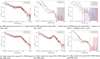 |
Fig. A.1 Event-pattern and -TM selection effects for three optically bright stars: eps Eri (#13, K2V star with G3.5 mag), π3 Ori (#34; F6V star with G3.2 mag), andβ Hy (#38; G0V subgiant with G2.7 mag). |
Best-fit parameters for FGK stars using different stacking strategies.
Appendix C Spectrum extraction for individual sources
The extraction of source and background was carried out with srctool (Brunner et al. 2022), with source and background radius adaptively chosen for detected source (exttype=AUTO) and fixed radius (source radius: 45″, background annulus radius: 60″, 99″) for the undetected sources (exttype=POINT). The fixed 45″ sources radius is about 3 time of the HEW of SRG/eROSITA survey mode. For the detected sources, the automatically determined source and background radii take into account the PSF, the detected counts, the background level, and the detection likelihood. A few customized settings for the AUTO mode of srctool we used are listed in Table C.12.
Amongst these settings, the most important is SRCTOOL_ AUTOREG_BACK_TO_SRC_AREA_RATIO, which defines the background region to be three times larger than the source region. The detection status of the stars was determined by cross-matching with the eRASS:1 catalogue (Merloni et al. 2024), selecting the nearest source within 15″, followed by visual inspection. In cases where additional X-ray sources were present within the extraction region, they were masked using circular regions with radii equal to twice the APERTURE radius from the catalogue to minimize contamination from nearby sources.
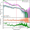 |
Fig. A.2 X-ray stacked spectra for the optically-bright M dwarf stars (orange: mG < 10), optically-faint (blue: mG > 10) M dwarf stars, optically-bright FGK dwarf stars (green: mG < 5) and optically-faint (violet: mG > 5) FGK dwarf stars. The middle and bottom panels display the ratio between the two groups of spectra. |
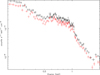 |
Fig. A.3 Comparison between the original M stacked spectrum (black) and that obtained after excluding the central 5″ region from each source (red). |
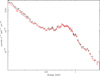 |
Fig. A.4 Comparison between the original FGK stacked spectrum (black) and that obtained after excluding the central 5″ region from each source (red). |
Appendix D More configuration of elemental abundance for VAPEC
Here we show the result from fitting M dwarf stars with 1T-VAPEC and 2T-VAPEC (Table D.1 and D.2 respectively) using different initializations for the metal abundances. Parameters fixed to a number or to another parameter are shown by the = symbol. We adopt model C in the main text because it provides good fits for both the M- and FGK-star samples without imposing an arbitrary fixed He abundance or yielding unphysical parameter values. We note, however, that alternative model configurations may also be plausible.
SRCTOOL autoregistration parameters.
Fits of M dwarf with 1T-VAPEC using different initializations for the metal abundances.
Appendix E bootstrap resampling
Besides the fit uncertainty, we perform a bootstrap resampling to estimate the uncertainty on the fit values by computing their scatter across the different realizations. This is a repeatable resampling from the full stars that form the same volume. In practice, we do 1000 realization. After stacking and fitting again every realization, we derive systematic uncertainties on each parameter by [5%, 95%] confidence intervals (90% CI) from the obtained distribution of their values. The corresponding values are reported in the fit summary tables presented as Table 2 for M stars and Table 6 for FGK stars.
Fits of FGK dwarf with 2T-VAPEC using different initializations for the metal abundances.
Appendix F Luminosity in single eRASS
Figure F.1 shows the variation in the average X-ray luminosity of nearby M (top) and FGK (bottom) dwarfs across the four eROSITA all-sky surveys (eRASS1 to eRASS4). The overall consistency indicates that the mean luminosities derived for the 10-pc M- and FGK-dwarf samples defined in WGH are stable over time and not significantly affected by temporal variability.
Appendix G Assessing log-normal DEM models for M and FGK spectra
We test to fit the average spectra with a multi-temperature plasma model that represents the emission as a log-normal distribution of APEC components, namely lognorm3. It approximates the differential emission measure by summing N discrete temperature components (default N=21) with temperatures evenly spaced in lnT. Each component is weighted by ![Mathematical equation: $w_i \propto \exp\!\left[-\frac{1}{2}\left(\frac{\ln T_i-\ln T_{\rm c}}{\ln\sigma}\right)^2\right]$](/articles/aa/full_html/2026/05/aa57865-25/aa57865-25-eq183.png) . As the width parameter decreases, the distribution approaches a single-temperature apec model. In Table G.1, we show that the single-lognorm fits improve upon the 1T-APEC and 1T-VAPEC models, but the overall fit quality remains poor. While the two-lognorm model provides acceptable fits for both stellar groups, it does not outperform the 2T-APEC model and yields poorly constrained width parameters (logsigma). We therefore find no statistically compelling evidence that lognorm models are required to describe the spectra.
. As the width parameter decreases, the distribution approaches a single-temperature apec model. In Table G.1, we show that the single-lognorm fits improve upon the 1T-APEC and 1T-VAPEC models, but the overall fit quality remains poor. While the two-lognorm model provides acceptable fits for both stellar groups, it does not outperform the 2T-APEC model and yields poorly constrained width parameters (logsigma). We therefore find no statistically compelling evidence that lognorm models are required to describe the spectra.
A further insight from the single-lognorm fits is that they help explain the unrealistically low abundances obtained in the 1T case. For the M-star spectrum, the 1T-APEC fit yields Z=0.061, well below the ∼0.1-1 Z⊙ found in optical and infrared studies of local M dwarfs (Montes et al. 2018; Neves et al. 2012; Woolf & Wallerstein 2005). This experiment with lognorm supports the interpretation that the extremely low metallicity is an artefact of modelling an intrinsically multi-temperature spectrum with an oversimplified 1T model.
Appendix H Table of all stars
Table H.1 and Table H.2 list the full set of stars included in our analysis and initially identified and catalogued by Caramazza et al. (2023). For each object, the table provides the identifier, coordinates (RA and DEC) at J2020, distance in parsecs, spectral type, Gaia G-band magnitude, and a flag indicating whether the source is detected in the eRASS1 catalogue (denoted as IF_ERASS. The final column gives additional comments, including cross-matches with commonly known catalogue names. Distance in pc are computed as 1000/PARALLAX (mas), where the parallax values are taken from Gaia EDR3 (Reylé et al. 2021). Their 10 pc sample also includes stars slightly beyond 10 pc (e.g. 10.2 pc), whose parallax uncertainties make them statistically consistent with being within 10 pc.
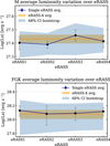 |
Fig. F.1 Average X-ray luminosity variation of nearby M (top) and FGK (bottom) dwarfs over the four eROSITA all-sky surveys (eRASS1 to eRASS4). Blue points represent the average luminosity from individual eRASS epochs, with vertical bars indicating the methodological uncertainties. The orange horizontal band shows the average luminosity obtained from the combined eRASS:4 spectra, while the shaded blue area indicates the 68% confidence interval estimated via bootstrap resampling. |
Fits using model lognorm.
Gaia 10 pc M stars. Rate_e1 denotes the eRASS1 catalogue count rate (Merloni et al. 2024), taken from the column ML_RATE_0_e1, i.e., the 0.2-2.3 keV band rate. a: Flag A - field crowded; Flag B - optical loading; Flag C- close pair. Detailed definition see Section 2.
Gaia 10 pc FGK stars. Rate_e1 denotes the eRASS1 catalogue count rate (Merloni et al. 2024), taken from the column ML_RATE_0_e1, i.e., the 0.2-2.3 keV band rate. Flag A: field crowded; Flag B: optical loading; Flag C: close pair.
All Tables
Sample selection in this work based on Gaia 10-pc M-type and F-, G-, and K-type stars (Stelzer, priv. comm.).
Fits of M dwarf with 1T-VAPEC using different initializations for the metal abundances.
Fits of FGK dwarf with 2T-VAPEC using different initializations for the metal abundances.
Gaia 10 pc M stars. Rate_e1 denotes the eRASS1 catalogue count rate (Merloni et al. 2024), taken from the column ML_RATE_0_e1, i.e., the 0.2-2.3 keV band rate. a: Flag A - field crowded; Flag B - optical loading; Flag C- close pair. Detailed definition see Section 2.
Gaia 10 pc FGK stars. Rate_e1 denotes the eRASS1 catalogue count rate (Merloni et al. 2024), taken from the column ML_RATE_0_e1, i.e., the 0.2-2.3 keV band rate. Flag A: field crowded; Flag B: optical loading; Flag C: close pair.
All Figures
|
Fig. 1 Left: X-ray luminosity (0.1-2.4 keV) versus Gaia GBP-GRP colour for the eRASS1-detected M- and FGK-type stars (Merloni et al. 2024) in the western Galactic hemisphere of the 10-pc Gaia sample. Filled blue circles: eRASS1-detected M dwarfs (l ≥ 180°); filled red circles: eRASS1-detected FGK stars (l ≥ 180°). Notable sources are labeled. Right: eRASS:4 total observed counts in 0.2-2.0 keV versus the distance from the Sun for the 10-pc Gaia sample in the western Galactic hemisphere, with detections and non-detections for M dwarfs (blue, cyan) and FGK stars (brown, coral). |
| In the text | |
|
Fig. 2 Histogram of Gaia G apparent (G, filled bars) and absolute (MG, outlined bars) magnitudes of the M-type (blue) and FGK-type (red) stars used in this study. The G mag and parallax were taken from Reylé et al. (2021). Five stars with Gaia- saturated magnitudes are not shown here. The vertical dashed line marks the optical loading threshold adopted in this work (G > 5; Robrade, priv. comm.). |
| In the text | |
|
Fig. 3 Comparison of effective area of TM8. The box plot represents the statistical distribution of the mean effective area over the 0.2-2.0 keV range. The solid horizontal lines within each box indicate the average value, while the dashed horizontal line (in the zoomed-in plot) represents the median. The sample includes all 103 M stars and 30 FGK stars used in this study. |
| In the text | |
|
Fig. 4 Left panel: averaged 10-pc M-dwarf spectrum with different models. All the models are labelled in the legend, where names follow the XSPEC convention, and the letter G stands for the Gaussian components used to fit single emission lines (dotted lines). Right panel: temperature versus line ratio assuming a single thermal component. The dark red and navy lines show the expected O VIII/OVII and NeX/NeIX ratios from AtomDB. Vertical dashed and dotted lines mark ratios derived from Gaussian normalisations in Table 2. |
| In the text | |
|
Fig. 5 Model fitting of the averaged X-ray spectra (0.2-2.0 keV) of 103 M-dwarf stars using multi-temperature thermal plasma models. The top left, top right and bottom left panels show comparisons between two-temperature and three-temperature APEC models (labelled as 2APEC and 3T-APEC), and as variable-abundance counterparts (2T-VAPEC and 3T-VAPEC). The corresponding residuals are shown. The bottom right panel presents a comparative view of residuals amongst four models to assess the fit quality. |
| In the text | |
|
Fig. 6 Comparison between X-ray brightness sub-groups and sub-spectral-type groups. All spectra are normalised to a distance of 10 pc and aligned at 0.7 keV for comparison. Each spectrum is fitted with a 2T-APEC model. The residual ( |
| In the text | |
|
Fig. 7 Model fitting of averaged X-ray spectra of 30 FGK stars (0.35-2.0 keV) using multi-temperature thermal plasma models. The four panels compare the performance of two-temperature and three-temperature APEC and VAPEC models, with corresponding residuals shown below each spectrum. The corresponding residuals are shown. |
| In the text | |
|
Fig. 8 Comparison of spectra of 103 M stars (orange) and 30 FGK stars (green) in the 10-pc Gaia sample. Models 2T-apec and 2T-VAPEC were applied, respectively. The middle panel displays the residual of the fit. The bottom panel shows the ratio between the average FGK and 5.55 times brighter M-star spectra. The scale comes from the ratio of luminosity in 0.2-2.0 keV. The Poisson noise is applied. |
| In the text | |
|
Fig. A.1 Event-pattern and -TM selection effects for three optically bright stars: eps Eri (#13, K2V star with G3.5 mag), π3 Ori (#34; F6V star with G3.2 mag), andβ Hy (#38; G0V subgiant with G2.7 mag). |
| In the text | |
|
Fig. A.2 X-ray stacked spectra for the optically-bright M dwarf stars (orange: mG < 10), optically-faint (blue: mG > 10) M dwarf stars, optically-bright FGK dwarf stars (green: mG < 5) and optically-faint (violet: mG > 5) FGK dwarf stars. The middle and bottom panels display the ratio between the two groups of spectra. |
| In the text | |
|
Fig. A.3 Comparison between the original M stacked spectrum (black) and that obtained after excluding the central 5″ region from each source (red). |
| In the text | |
|
Fig. A.4 Comparison between the original FGK stacked spectrum (black) and that obtained after excluding the central 5″ region from each source (red). |
| In the text | |
|
Fig. F.1 Average X-ray luminosity variation of nearby M (top) and FGK (bottom) dwarfs over the four eROSITA all-sky surveys (eRASS1 to eRASS4). Blue points represent the average luminosity from individual eRASS epochs, with vertical bars indicating the methodological uncertainties. The orange horizontal band shows the average luminosity obtained from the combined eRASS:4 spectra, while the shaded blue area indicates the 68% confidence interval estimated via bootstrap resampling. |
| In the text | |
Current usage metrics show cumulative count of Article Views (full-text article views including HTML views, PDF and ePub downloads, according to the available data) and Abstracts Views on Vision4Press platform.
Data correspond to usage on the plateform after 2015. The current usage metrics is available 48-96 hours after online publication and is updated daily on week days.
Initial download of the metrics may take a while.