© The Authors 2026

1. Introduction

The Kepler mission observed many stars, which enabled the detection and interpretation of solar-like oscillations in red giants. Solar-like oscillations are stochastically excited by the turbulent convection in the outer layers of the stars. The restoring force of the radial oscillation (ℓ = 0) modes is the pressure gradient. These oscillations are referred to as pressure (p) modes. In the case of non-radial modes (ℓ > 0), the pressure modes in the outer parts of the star couple with modes in the core of the red-giant stars where buoyancy is the restoring force. These oscillations are referred to as mixed modes. The set of radial and non-radial modes are thus sensitive to different parts of the stars, which provides a wealth of information on the stellar structure (e.g. Bedding et al. 2011; Beck et al. 2012; Stello et al. 2016; Mosser et al. 2017; Hekker et al. 2018; Pinçon et al. 2020; Lindsay et al. 2023).

An essential ingredient in the use of oscillations to determine the internal stellar structure is the identification of the radial order (n), the spherical degree (ℓ), and, for non-radial modes, the azimuthal order (m). In the case of solar-like oscillations in red-giant stars, the frequencies of low-degree (ℓ = 0, 1, 2, 3) modes appear in a pattern that shows similarities – though with some changes due to the appearance of mixed modes – with the low-degree mode pattern observed in the Sun. This pattern can be described by the asymptotic relation as developed by Tassoul (1980), as the observed low-degree modes are in the asymptotic limit with ℓ ≪ n. However, the radial order of the observed modes decreases with evolution, and hence for red-giant stars it becomes questionable if the asymptotic approximation is still valid. In practice, this means that increasing deviations from the asymptotic relation are expected with the evolution of stars on the red-giant branch (RGB). These deviations reduce again in the core-helium-burning phase as the observed oscillations in these stars occur at higher radial orders compared to the oscillations in stars high on the RGB.

To account for the expected deviations from the asymptotics, Mosser et al. (2011) adapted the asymptotic relation developed by Tassoul (1980) by adding a second-order term (indicated in blue),

$$\begin{array}{c}\hfill {\nu }_{n,\ell }=\mathrm{\Delta }\nu (n+\frac{\ell }{2}+{ϵ}_{\mathrm{p}}+\mathit{blue}\frac{\alpha }{2}{(n-n_{\max })}^2)+d_{0,\ell },\end{array}$$(1)

for the eigenfrequencies ν_n, ℓ, where Δν is the asymptotic large-frequency separation – i.e. the typical frequency difference between modes of the same degree and consecutive radial order –, ϵ_p is a phase term, and d_0, ℓ a small correction to the leading order asymptotics, which is zero for ℓ = 0 modes. In the second-order term, indicated in blue, α accounts for the frequency-dependent deviation from the regular pattern set by Δν and is often referred to as ‘curvature’. Finally, n_max is the radial order¹ of the frequency of maximum oscillation power (ν_max). See Fig. 1 for a so-called échelle diagram in which the curvature is illustrated.

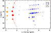Fig. 1. Échelle diagram of KIC 2443903 with the degrees of the modes indicated with different colours as per the legend. The curvature, i.e. not straight, vertical orientation of the radial modes is highlighted with the dashed red line.

Mosser et al. (2011, 2012, 2013a,b) have derived several prescriptions for α in stars with Δν < 20 μHz. The most recent one is

$$\begin{array}{c}\hfill \alpha =0.015\mathrm{\Delta }{\nu }^{-0.32}=0.09n_{\max }^{-0.96}\approx 2a_{\mathrm{RG}}{n}_{\max }^{-1},\end{array}$$(2)

where $\mathrm{\Delta }\nu \propto {\nu }_{\max }^{0.75}$ (e.g. Hekker et al. 2011), and the value of a_RG = 0.038 ± 0.002 was obtained from a fit; see Mosser et al. (2013a,b) for more details and Vrard et al. (2015) for an application.

In this work, we aim to take the next step in the determination and interpretation of the curvature. Our first aim is to determine α and Δν in a homogeneous manner for all red giants that exhibit a sufficient number of detected radial modes (see Sect. 2 for a more precise discussion of the criteria). We then compare the curvature values obtained from observed red giants with curvature values obtained from models (Sects. 3 and 4). Finally, we computed the sensitivity of the curvature to the internal structure of the stars (Sect. 5) and linked this to features of the internal structure (Sect. 6). We provide our discussion and conclusions in Sect. 7.

2. Analysis of curvature in observations

For the observations, we used the Kepler light curves prepared with the method described by Handberg & Lund (2014) for the 6661 stars from the APOKASC Data Release 2 (DR2) catalogue (Pinsonneault et al. 2018). To be sure that we were comparing like for like, we only used stars for which the available time series is at least 1200 days long, with a filling factor larger than 65%, throughout this study. These time-series data were subsequently analysed using the Tools for the Automated Characterisation of Oscillations (TACO) code (Themeßl et al. 2020; Hekker et al., in prep.). In TACO, the time-series data are converted to the frequency domain using a Fourier transformation. TACO then performs a global fit to the resulting power density spectrum (PDS) following the prescription in Kallinger et al. (2014). This global fit includes three Lorentzian-like functions each, with an exponent of four to account for background signal (instrumentation and granulation at different scales), white noise, and a Gaussian-shaped oscillation power excess. The PDS is subsequently normalised by the background and white-noise part of this global fit. This left us with a normalised PDS, where the oscillations are the dominant signal. Finally, TACO fits all significant peaks in the relevant frequency range of the PDS and locates the radial modes in this normalised spectrum using the regularity in the frequencies of the oscillation modes as expressed in Eq. (1).

For a meaningful comparison of the values of α between different stars, as well as between stars and models, we compiled a sample of stars that have at least six radial modes observed and identified. For stars with more than six radial modes, we used the six modes closest to ν_max. This provides us with a homogeneous sample. The selection of six modes is empirically determined and provides a balance between having enough stars with enough radial modes identified and having robust determinations of α; i.e. a sufficient number of modes to measure the curvature.

Based on these requirements and omitting some stars with unusual features, such as high complexity (Choi et al. 2025) in their PDSs, we present here a sample of 2242 RGB stars and 1698 core-helium-burning (CHeB) stars. The evolutionary stages were taken from the APOKASC DR2 catalogue (Elsworth et al. 2019).

2.1. Determination of α

The second-order term in Eq. (1) introduces two additional parameters (α & n_max). To avoid explicit correlations with other parameters such as ν_max, we opted to eliminate n_max from the fitting. We therefore rewrote Eq. (1) for radial modes, i.e. ℓ = 0, as a general second-order equation:

$$\begin{array}{c}\hfill {\nu }_{n,\ell =0}=A{n}^2+Bn+C,\end{array}$$(3)

with

$$\begin{array}{cc}\hfill A& =\mathrm{\Delta }\nu \frac{\alpha }{2}\hfill \end{array}$$(4)

$$\begin{array}{cc}\hfill B& =\mathrm{\Delta }\nu (1-\alpha n_{\max })\hfill \end{array}$$(5)

$$\begin{array}{cc}\hfill C& =\mathrm{\Delta }\nu ({ϵ}_p+\frac{\alpha n_{\max }^2}{2}).\hfill \end{array}$$(6)

To obtain α, we fitted the radial mode frequencies using Eq. (3) to obtain values for A, B, and C. To use A to derive an estimate of α, we need a value for Δν, which we determined from a linear fit of the frequencies to the radial orders (ν_{n, ℓ = 0} = Δν(n + ϵ_p)). In essence, this minimises the variance in ν modulo Δν; i.e. the ridges in an échelle diagram (see Fig. 1) are assumed to be vertical straight lines to first order. We note that this is a different way of fitting the universal pattern (Eq. (1)) as compared to earlier works by, for example, Mosser et al. (2013a), which may alter the values obtained for α as well as Δν. The approach we adopted here does not require a value of n_max, though it implicitly leads to the curvature being somewhere around the mean value of n. This implicit value of n_max only depends on the oscillation frequencies used and not on the determination and uncertainties in ν_max.

2.2. The α–Δν relation

In Fig. 2 we show the values of α derived using Eq. (3) as a function of Δν for RGB stars as well as for stars in the CHeB phase. Based on the morphology of the points in the left panel of Fig. 2, we fitted a linear relation in log α as a function of Δν, i.e.

$$\begin{array}{c}\hfill log\alpha =d_1\mathrm{\Delta }\nu +d_2.\end{array}$$(7)

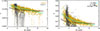Fig. 2. Curvature (α) as a function of the large frequency separation, with α plotted on a logarithmic scale (left) and a linear scale (right). See the legend for the meanings of the colours.

In Table 1 we list the values of d₁ and d₂ for both RGB and CHeB stars.

In Fig. 2 we also show the α − Δν relationship proposed by Mosser et al. (2012); see Eq. (2). We note that this fit overestimates the values at higher Δν and underestimates α at lower values of Δν. It should, however, be noted that the formulation for α versus Δν proposed by Mosser et al. (2012) was derived over a decade ago, at a time when the time-series data available were of a shorter duration than those used in this study. This may have led to a smaller number of radial modes being detected and higher uncertainties on the determined frequencies. Indeed, for higher values of α as found at low Δν, a fit to a smaller number of modes is likely to underestimate the value of α. It may well be that the six radial modes used in this work are also not sufficient to obtain the actual value of α in these cases. However, this issue remains elusive as the number of modes is limited for evolved stars due to the low radial order. Finally, as mentioned above, we fitted the universal pattern in a different way, which may impact both α and Δν.

2.3. Mass and metallicity dependence of α

Now that we have shown how α depends on Δν, we turn to other stellar parameters: mass and metallicity. In Fig. 3 we show the curvature versus large frequency separation colour-coded by mass and metallicity for the RGB and CHeB stars.

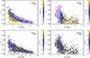Fig. 3. Curvature (α) as a function of the large-frequency separation (Δν) for RGB stars (left) and CHeB stars (right), colour-coded by mass (top) and metallicity (bottom).

2.3.1. Mass dependence.

For CHeB stars, it is well known that there is a strong dependence between mass and Δν (see e.g. Mosser et al. 2014), and indeed we recover this trend in Fig. 3. We do not find any particular variation in α with mass at fixed Δν. For the RGB stars, the situation is different. We find that at any value of Δν, α depends inversely on mass; i.e. α increases with decreasing stellar mass. We investigated this mass dependence using the models described later in this paper.

2.3.2. Metallicity dependence.

There does not seem to be any dependence of α on metallicity for either the RGB or the CHeB stars. Though, in the case of the CHeB stars, this might be due to observational biases, as this sample is dominated by stars with solar metallicity. Certainly for the higher mass stars in the secondary clump, the variation in metallicity is too small to draw any conclusions on a potential metallicity dependence of α. For the RGB stars, the spread in metallicity is larger than for the secondary clump, though it is still relatively narrow, with values between −0.6 and 0.4 dex. For these values, the metallicity independence seems robust.

3. Analysis of curvature in stellar models

To compare the curvature results from the observations with predictions, we also analysed stellar models for the curvature using the Modules for Experiments in Stellar Astrophysics (MESA) code, version r12778 (see Paxton et al. 2011, 2013, 2015, 2018, 2019; Jermyn et al. 2023, and references therein). We used the standard settings, i.e. the solar composition from Grevesse & Sauval (1998); the mixing-length parameter was kept to the value of two, as per the default; convective boundaries were chosen according to the Schwarzschild criterion, with no overshoot, no diffusion, nor settling of helium and heavy elements. The oscillation frequencies of radial modes were computed using GYRE (Townsend & Teitler 2013; Goldstein & Townsend 2020, and references therein). We computed solar metallicity tracks with masses of 0.8, 1.0, 1.3, 1.6, 1.9, and 2.2 M_⊙. Additionally, we computed 1.0 M_⊙ tracks with metallicities of [Fe/H] = −0.5, −0.2, 0.0, 0.2, and 0.35 dex.

To mimic the observations, we selected the six radial mode frequencies closest to ν_max. We subsequently used the selected frequencies to obtain α from Eq. (3). For the models, we computed ν_max from the scaling relation, i.e. ${\nu }_{\max }\propto M{R}^{-2}{T}_{\mathrm{eff}}^{-0.5}$, with M, R, and T_eff in solar units, where T_eff, ⊙ = 5777 K (Prša et al. 2016), and a reference value for ν_max of 3100 μHz (see Hekker 2020 and references therein for a discussion on the reference values for scaling relations).

To account for uncertainties, we perturbed ν_max randomly, assuming a 5% uncertainty. We imposed this perturbation to allow a change in the set of six modes that were selected and used to determine the curvature. Additionally, we introduced an uncertainty on the individual frequencies. For this, we used the quadratic uncertainty model centred around ν_max described by Ahlborn et al. (2025). To investigate the effect of these uncertainties on the derived values of α and Δν, we performed a Monte Carlo analysis for some individual models. We found that the resulting uncertainties in α and Δν align with typical observed uncertainties; see Appendix B for more details. We show the α versus Δν results for the stellar models in Fig. 4.

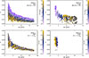Fig. 4. Same as Fig. 3 for results based on our stellar model computations. Note that in the top panels all models have solar metallicity, while in the bottom panels we show only one mass. The latter is the cause of the reduced frequency range of models in panel d.

Figure 4 shows that α typically increases with decreasing Δν for both the RGB and CHeB models. We discuss the mass and metallicity trends in these models below.

3.1. Mass dependence.

For the RGB stars, the models show a clear mass trend, with lower mass stars having more curvature (larger values of α) at the same Δν. To investigate this further, we performed linear fits in log α versus Δν for individual mass tracks; see Eq. (7). We did this by fitting both the slope (d₁) and the intercept (d₂), as well as by fixing the slope and only fitting the intercept. The value to which we fixed the slope was the value of d₁ obtained from a fit including all models of all mass tracks. We show the intercepts as a function of mass in Fig. 5. The intercept indeed decreases with mass (this trend is irrespective of the slope), confirming that the curvature decreases with stellar mass. For the CHeB stars, the well-known mass dependence with Δν was recovered (see Fig. 4).

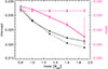Fig. 5. Intercepts (dark grey, left axis) and slopes (pink, right axis) of linear fits in log α versus Δν for RGB models as a function of mass. The points show the mean slope and intercept of fits for 1000 perturbations in which we perturbed both νmax and the individual frequencies within their uncertainties. The vertical bars indicate the spread in the results of these 1000 perturbations. The points connected by a solid line show the results of fits in which both the slope and the intercept were free parameters. The dashed lines connect points for fits with a fixed slope. See text for more details and Fig. C.1 for the fits to the different masses.

3.2. Metallicity dependence.

For the stars on the RGB nor for stars in the CHeB phase, is there a trend between metallicity and α.

4. Comparing α from observations and models

A comparison of the top rows of Figs. 3 and 4 shows that the models qualitatively confirm the trends seen in the observations. To quantify this, we selected two observational samples: a solar-metallicity ([Fe/H] = 0.0 ± 0.1 dex) sample, and a solar-mass (M = 1.0 ± 0.1 M_⊙) sample. We subsequently performed a coarse grid-based modelling in which we selected a model for each observed star in the two samples. For the solar-metallicity sample, we selected models from the [Fe/H] = 0 tracks that are closest to the observed mass and Δν. For the solar-mass sample, we selected models from the 1 M_⊙ tracks that are closest to the observed metallicity and Δν. In Fig. 6 we show the results for both the observed samples, as well as their respective models.

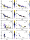Fig. 6. Curvature (α) as a function of the large frequency separation (Δν) for observations (left) and models (right), split for RGB stars (panels a–d) and CHeB stars (panels e–h), colour-coded by mass (panels a–b and e–f) and metallicity (panels c–d and g–h). The colour code is the same for both the observations and the models. The black lines indicate the RGB and CHeB fits from Fig. 2 and Eq. (7), with the coefficients from Table 1, except for panels c and d, where we use a fit through the selected observed values to account for the dependence of α on mass.

For the CHeB stars, we find that the fit through the data does indeed overlap with the models; however, the values of α for the solar metallicity models are somewhat higher than those observed. For RGB stars on the other hand, this picture is rather different; the models seem to be offset in α and have a different slope of α versus Δν. This is most pronounced in Fig. 6d, where the majority of the solar-mass models lie above the fit and the offset from the fit increases with increasing Δν.

It is known that the frequencies of stellar models must be corrected for the surface effect – the inability of the models to properly reproduce the conditions near the stellar surface (Kjeldsen et al. 2008; Ball & Gizon 2014). We therefore investigated if the discrepancy in α between the observations and the models is due to this phenomenon. We did this in two different ways. We first performed a quantitative analysis by including a surface correction δν_s with an arbitrary shape as a function of n into Eq. (1). From this, one can derive a relation between the modelled value of α (α_mod) and the corrected α (α_c), which should, in the ideal case, be the same as the observed α (α_obs):

$$\begin{array}{c}\hfill {\alpha }_{\mathrm{obs}}\approx {\alpha }_{\mathrm{c}}\approx {\alpha }_{\mathrm{mod}}\frac{\mathrm{\Delta }{\nu }_{\mathrm{mod}}}{\mathrm{\Delta }{\nu }_{\mathrm{obs}}}+\frac{1}{\mathrm{\Delta }{\nu }_{\mathrm{obs}}}\frac{d^2\delta {\nu }_s}{\mathrm{d}{n}^2};\end{array}$$(8)

see Appendix A for the derivation of Eq. (8). The known shape of the surface corrections implies that Δν_mod > Δν_obs (e.g. Ball & Gizon 2014). Thus, for the larger values of α_mod compared to α_obs to be explained by the surface effect, the second-order derivative of δν_s needs to be negative. We used the Sun, the main-sequence stars from Buchele et al. (2024, 2025), and RGB stars from Ball et al. (2018) to test this (see Appendix A for details). Indeed, we find that a negative value for this derivative is likely and thus that the surface effect could be responsible for the discrepancy between α_obs and α_mod. To take this qualitative result one step further and quantify if the surface correction is indeed the culprit, we also used surface-corrected models from Li et al. (2023) to investigate the impact of the surface correction on α.

Li et al. (2023) performed a study in which they computed the a₃ and a₋₁ coefficients for the surface effect described in Ball & Gizon (2014) based on stellar parameters, i.e. surface gravity, effective temperature, and metallicity. They also made a grid of models publicly available in which their surface effects are already included. Here, we used the models and frequencies from this grid and repeat the analysis of Sect. 3 with these models. We show the α − Δν relation for both the corrected and uncorrected frequencies as computed by Li et al. (2023) in Fig. 7. The uncorrected results of the top panel of Fig. 7 closely resemble Fig. 6d. For the surface-corrected results shown in the bottom panel of Fig. 7, the values of α are indeed reduced. However, the reduction seems to be too strong at lower values of Δν (i.e. Δν ≲ 7 μHz) and not strong enough for models with Δν ≳ 12 μHz. This could mean that the surface correction should be altered, or the surface correction is correct and there is some additional physics missing in the models. For the moment, we cannot distinguish between these options. However, if the latter assumption is true, it is important to know to which part of the star α is most sensitive. We discuss this in the next section.

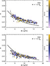Fig. 7. Same as Fig. 6d for uncorrected (top) and surface-corrected frequencies (bottom) using models from Li et al. (2023).

5. Dependence of the curvature on stellar structure features

To investigate to which part of the star the curvature is most sensitive, we used structure kernels following the approach described by Otí Floranes et al. (2005) and references therein. These authors examined the sensitivities of frequency ratios on the stellar structure. The idea is as follows: frequency differences between two sufficiently similar stellar models (or between an observed star and a sufficiently close model) can typically be expressed in terms of differences in two structure variables, for example squared sound speed (c²) and density (ρ). The frequency differences and structure differences are connected through kernel functions. These kernel functions quantify how changes to the stellar structure translate into changes in the pulsation frequencies; i.e. the kernel functions indicate the sensitivity of a structure parameter as a function of a given stellar coordinate. The latter is often (though not necessarily) expressed in fractional radius. Using these kernels, differences in frequencies can now be ‘translated’ into differences in internal structures through their kernels.

To find the sensitivity of α, we write Eq. (1) for ℓ = 0 modes and define x = n − n_max to obtain

$$\begin{array}{c}\hfill {\nu }_{x+n_{\max },0}=\mathrm{\Delta }\nu (x+n_{\max }+{ϵ}_p+\frac{\alpha }{2}{x}^2).\end{array}$$(9)

Taking the derivative with respect to x yields

$$\begin{array}{c}\hfill \frac{\mathrm{d}{\nu }_{x+n_{\max },0}}{\mathrm{d}x}=\mathrm{\Delta }\nu +\alpha \mathrm{\Delta }\nu x,\end{array}$$(10)

where n_max and ϵ_p are assumed to be constant with respect to x. To solve this equation, we need a value for n_max, which we obtained from n_max = ν_max/Δν − ϵ_p. We checked differences in values for Δν and α obtained from Eqs. (3) and (10). The differences in Δν are well below 1%. The differences in α are larger, though at least one order of magnitude smaller than the actual values. Equation (10) is a linear relationship:

$$\begin{array}{c}\hfill y={\beta }_0+{\beta }_{1}x,\end{array}$$(11)

with the intercept β₀ = Δν and the slope β₁ = αΔν. To obtain α, we can divide the slope (β₁) through the intercept (β₀):

$$\begin{array}{c}\hfill \alpha =\frac{\alpha \mathrm{\Delta }\nu }{\mathrm{\Delta }\nu }=\frac{{\beta }_1}{{\beta }_0}·\end{array}$$(12)

Following Otí Floranes et al. (2005), we wrote the linearised perturbations in α, denoted by δα, as a function of the perturbations in αΔν (δ(αΔν)) and Δν (δΔν) as

$$\begin{array}{c}\hfill \delta \alpha =\frac{1}{\mathrm{\Delta }\nu }(\delta (\alpha \mathrm{\Delta }\nu )-\alpha \delta \mathrm{\Delta }\nu ).\end{array}$$(13)

The kernel for differences in α, i.e. ${\underline{K}}_{\alpha }$, is therefore

$$\begin{array}{cc}\hfill {\underline{K}}_{\alpha }& =\frac{1}{\mathrm{\Delta }\nu }({\underline{K}}_{\alpha \mathrm{\Delta }\nu }-\alpha {\underline{K}}_{\mathrm{\Delta }\nu })\hfill \end{array}$$(14)

$$\begin{array}{cc}& =\frac{1}{\mathrm{\Delta }\nu }({\underline{K}}_{{\beta }_1}-\alpha {\underline{K}}_{{\beta }_0}),\hfill \end{array}$$(15)

where $\underline{K}\equiv [K^{c^2},K^{\rho }]$, with K^c2 and K^ρ being the sensitivity kernels for sound speed (c) and density (ρ), respectively (for the derivations of these kernels, see e.g. Gough & Thompson 1991; Kosovichev 1999; Basu 2016). These kernels were determined by the structure and mode frequencies of the models².

To obtain ${\underline{K}}_{{\beta }_0}$ and ${\underline{K}}_{{\beta }_1}$, we used the linear expression of Eq. (11) again. This linear regression can conveniently be written in matrix notation:

$$\begin{array}{c}\hfill \mathbf{Y}=\beta ·\mathbf{X},\end{array}$$(16)

with Y = (dν₁/dx₁, …, dν_N/dx_N)^T, X = (x₁, …x_N), and β = (β₀, β₁)^T. The values for Y were determined as the frequency differences between radial modes with consecutive radial orders, and X are the radial-order differences of these eigenfrequencies. For this analysis, we selected (from the models described in Sect. 3) a subset with two different masses (M = 1.0 and 1.9 M_⊙) and a sufficient number of radial modes. That is, we set N = 6 to include the six modes closest to ν_max, consistently with what was used for the observations and models presented in Sects. 2 and 3 of this work. Following Ahlborn et al. (2022), we determined β by means of linear regression, and the parameters are estimated as

$$\begin{array}{c}\hfill \beta ={({\mathbf{X}}^T·\mathbf{X})}^{-1}\mathbf{X}·\mathbf{Y}=\mathbf{C}·\mathbf{Y}.\end{array}$$(17)

The matrix C can be interpreted as a coefficient matrix, i.e. with the coefficients c_βj, determining the impact (weight) of each data point on the derived parameters β_j, while Y is the difference in consecutive frequencies. So, we can write this as

$$\begin{array}{c}\hfill {\beta }_j=\sum _{i\in \mathcal{M}}{c}_{{\beta }_j,i}({\nu }_{i+1}-{\nu }_i).\end{array}$$(18)

We can use this to construct sensitivity kernels for the slope (β₁) and the intercept (β₀):

$$\begin{array}{c}\hfill {\underline{K}}_{{\beta }_j}=\sum _{i\in \mathcal{M}}{c}_{{\beta }_j,i}({\underline{K}}_{i+1}(r)-{\underline{K}}_i(r)),\end{array}$$(19)

where ℳ refers to the mode set of interest, and ${\underline{K}}_i(r)$ are the kernel functions of each oscillation mode, i.

We computed ${\underline{K}}_{\alpha }$ for several models along both the 1 M_⊙ and 1.9 M_⊙ tracks (see right panel of Fig. 9). For a representative model, we show ${\underline{K}}_{\alpha }$ in Fig. 8. The largest amplitude in ${\underline{K}}_{\alpha }$ is located relatively close to the stellar surface and overlaps with the dip in Γ₁, indicating the He I and H I ionisation layer. This is the case for all models we investigated. For reference, we also show the radial eigenfunction of the radial mode closest to ν_max in Fig. 8. This shows that the period of the eigenfunction at the combined He I and H I ionisation layer is of the same order or larger than the extent of this layer.

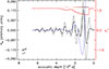Fig. 8. Kernels for α (${\underline{K}}_{\alpha }$) as a function of acoustic depth (black and grey) for a 1 M⊙ model with a νmax of about 76 μHz. For comparison, we also show Γ1, the first adiabatic exponent in red, as well as its deviation from 5/3 in the colour code just above it. For comparison, the dashed blue curve shows the radial eigenfunction of the radial mode closest to νmax in arbitrary units.

6. Dependence of α on characteristics of ionisation layers

In this section, we investigate if we can derive any information about the He I and H I ionisation layers from α. To do so, we first return to Eq. (1) and note that this equation was derived by Mosser et al. (2013a) as the observational counterpart of the asymptotic approximation by Houdek & Gough (2007). In Eq. (1), the curvature term replaces the degree independent part of the second-order term in Eq. (20) of Houdek & Gough (2007), which depends on the stratification near the surface (Gough 1986 and references therein). Indeed, Fig. 8 confirms the sensitivity of α to the near-surface layers. Additionally, in Fig. 8 we show that the local wavelength of the eigenfunction is of the same order as the extent of the He I and H I ionisation layers. As for other features that occur on length scales shorter than or comparable to the local wavelength, such as the previously studied He II ionisation layer (see e.g. Miglio et al. 2010; Mazumdar et al. 2014; Broomhall et al. 2014), we can treat the combined He I – H I ionisation layer as a glitch, despite it being a more borderline case. Such a glitch can be described as

$$\begin{array}{c}\hfill \delta \nu =A_{g}sin(4\pi {\tau }_g\nu +\varphi ),\end{array}$$(20)

with A_g being the amplitude, τ_g the period, and ϕ the phase, where the amplitude would to some extent correlate with the abundance of the hydrogen and helium in the ionisation zone (see Broomhall et al. 2014 for an analysis of helium abundances from the amplitudes of He II glitch signatures) and τ_g would correlate with the acoustic depth of these ionisation layers. We note here that the He II ionisation layer and base of the convection zone are located deeper in the star than the He I and H I layers. At these larger depths, α is much less sensitive, and these deeper features appear as variations with shorter periods (see e.g. the deviations of the red points from the dashed red line in Fig. 1), which can be neglected when studying α. To explore this further, we replaced the curvature term in Eq. (1) by Eq. (20) and obtained the following for radial modes:

$$\begin{array}{c}\hfill {\nu }_{n,0}=\mathrm{\Delta }\nu (n+{ϵ}_{\mathrm{p}})+A_{g}sin(4\pi {\tau }_g\nu +\varphi ).\end{array}$$(21)

To derive values for A_g and τ_g, we performed a Monte Carlo fit with 5000 iterations to perturbed frequencies of the same models as used in Sect. 5. We present the results of this fitting in Fig. 9, where we compare these values with the ones obtained through the methods described in Sects. 2 and 3. From this, we find that the values for τ_g are in line with the region close to the surface as identified by the kernel sensitivity; i.e. between 0.1 × 10⁴ s and 2 × 10⁴ s, as also shown in Fig. 8. Furthermore, the amplitudes (A_g) decrease with mass, while τ_g increases with mass, at a similar value for α (see Fig. 9).

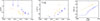Fig. 9. Amplitude (Ag, left) and acoustic depth (τg, centre) as a function of α for direct fits of Eq. (20) to the frequencies of models of 1 M⊙ (blue) and 1.9 M⊙ (orange). The bars indicate the 25th–75th percentiles of the distribution of the results of 5000 perturbations. The tracks evolve from left to right. The positions of the models in the Hertzsprung-Russell diagram are indicated with the dots in the right panel. The lines are the full tracks, shown to guide the eye.

To quantify this further, we attempted a Taylor expansion of the sinusoid up to the quadratic term to mimic Eq. (3), in Eq. (21), for which we converted the sinusoid to a cosine³ and used −A_gcosx = −A_g(1 − x²/2), with x = 4πτ_gν + ϕ and ν = Δν(n + ϵ_p) to obtain

$$\begin{array}{c}\hfill {\nu }_{n,0}=A_T{n}^2+B_{T}n+C_T,\end{array}$$(22)

with

$$\begin{array}{cc}\hfill A_T& =\frac{A_g}{2}{\left(4\pi {\tau }_g\mathrm{\Delta }\nu \right)}^2,\hfill \end{array}$$(23)

$$\begin{array}{cc}\hfill B_T& =\mathrm{\Delta }\nu +\frac{A_g}{2}\left(8\pi {\tau }_g\mathrm{\Delta }\nu (4\pi {\tau }_g\mathrm{\Delta }\nu {ϵ}_p+\varphi )\right),\hfill \end{array}$$(24)

$$\begin{array}{cc}\hfill C_T& =\mathrm{\Delta }\nu {ϵ}_p-A_g+\frac{A_g}{2}(4\pi {\tau }_g{ϵ}_p\mathrm{\Delta }\nu (4\pi {\tau }_g{ϵ}_p\mathrm{\Delta }\nu +2\varphi )+{\varphi }^2).\hfill \end{array}$$(25)

Equation (22) has the same shape as Eq. (3). As we derived α from the quadratic term in Eq. (3) only, we only included the quadratic term here. This provides

$$\begin{array}{c}\hfill \frac{A_g}{2}{\left(4\pi {\tau }_g\mathrm{\Delta }\nu \right)}^2=\frac{\alpha }{2}\mathrm{\Delta }\nu ;\end{array}$$(26)

thus,

$$\begin{array}{c}\hfill \alpha =A_g{(4\pi {\tau }_g)}^2\mathrm{\Delta }\nu .\end{array}$$(27)

As indeed both A_g and τ_g are included, this emphasises that α is determined by both the period and the amplitude of the He I and H I ionisation layers⁴. Upon checking this equality for the models, i.e α as determined in Sect. 3 and from using the right-hand side of Eq. (27), we indeed find reasonable agreement (see Fig. 10), empirically justifying the glitch approach. For higher values of α (α > 0.02), the agreement is not as good, potentially as for these higher values of α the six modes may not be enough to quantify the strong curvature and/or the glitch analysis with a Taylor expansion with only the quadratic term may no longer provide a proper approximation.

Fig. 10. Comparison of α determined via Eq. (3) versus the right-hand side of Eq. (27). The colours and lines have the same meanings as in Fig. 9.

These results, in which both the amplitude and the depth of the ionisation zones are intimately connected, prevent a direct determination of the location or the abundance of the near-surface ionisation zones from α. However, if this degeneracy can be lifted, and either the abundance or the location of the near-surface ionisation layers can be determined by other means, α can aid in finding the remaining unknown parameter.

7. Discussion and conclusions

In this paper, we present a way to obtain the curvature of the radial modes, i.e. the quadratic deviation of the modes from uniform spacing, in a homogeneous way. We did so without the need to compute the radial order of the frequency of maximum oscillation power (n_max) explicitly. The advantage of this approach is that the result relies only on the oscillation modes included. The observed values of the curvature have lower values than the ones obtained from stellar models. We investigated whether this is a result of the so-called surface effect. Indeed, if we include the surface effect, the overestimation of the models is reduced. However, a frequency-dependent offset remains. This may show that the surface correction needs to be improved, or it may be due to other physical shortcomings in the models. To investigate this further, we computed the sensitivity of the curvature, which is dominant in the combined He I and H I ionisation zone close to the stellar surface. The results of the sinusoidal approximation confirm this location. This proximity to the surface most likely means that this is entangled with the surface effect, although we clearly show that a state-of-the-art treatment of the surface effect does not fully mitigate the discrepancy between the observations and the models. From a Taylor expansion, we find that the curvature depends on both the amplitude and the period of the sinusoid. Hence, both the location and abundance of H and He play a role in the curvature.

Acknowledgments

We thank the referee and editor for their comments and work, which improved the manuscript significantly. We acknowledge funding from the ERC Consolidator Grant ‘DipolarSound’ (grant agreement # 101000296). SB is partially supported by NSF grant AST-2205026. YE acknowledges funding from the Science and Technology Facilities Council (STFC).

References

Appendix A: Surface effect

To gain insight in the direction and amount of the surface effect on α, we looked at the asymptotic description of radial modes (see Eq. (1)) and computed its derivatives to n:

$$\begin{array}{cc}\hfill {\nu }_n& =\mathrm{\Delta }\nu (n+{ϵ}_p+\frac{\alpha }{2}{(n-n_{\max })}^2),\hfill \end{array}$$(A.1)

$$\begin{array}{cc}\hfill \frac{\mathrm{d}{\nu }_n}{\mathrm{d}n}& =\mathrm{\Delta }\nu (1+\alpha (n-n_{\max })),\hfill \end{array}$$(A.2)

$$\begin{array}{cc}\hfill \frac{{\mathrm{d}}^2{\nu }_n}{\mathrm{d}{n}^2}& =\alpha \mathrm{\Delta }\nu .\hfill \end{array}$$(A.3)

We subsequently included a surface correction, δν_s, which is in this reasoning an arbitrary function of n which remains small enough such that the asymptotic description of radial modes is still valid. We call the corrected curvature, which should resemble the observations, α_c. From this, it follows that

$$\begin{array}{cc}\hfill {\nu }_n+\delta {\nu }_s& =\mathrm{\Delta }{\nu }_c(n+{ϵ}_{p,c}+\frac{{\alpha }_c}{2}{(n-n_{\max })}^2),\hfill \end{array}$$(A.4)

$$\begin{array}{cc}\hfill \frac{\mathrm{d}({\nu }_n+\delta {\nu }_s)}{\mathrm{d}n}& =\mathrm{\Delta }{\nu }_c(1+{\alpha }_c(n-n_{\max })),\hfill \end{array}$$(A.5)

$$\begin{array}{cc}\hfill \frac{{\mathrm{d}}^2({\nu }_n+\delta {\nu }_s)}{\mathrm{d}{n}^2}& ={\alpha }_c\mathrm{\Delta }{\nu }_c.\hfill \end{array}$$(A.6)

Now splitting the first term, we find

$$\begin{array}{cc}\hfill \frac{{\mathrm{d}}^2{\nu }_n}{\mathrm{d}{n}^2}+\frac{{\mathrm{d}}^2\delta {\nu }_s}{\mathrm{d}{n}^2}& ={\alpha }_c\mathrm{\Delta }{\nu }_c,\hfill \\ \hfill \alpha \mathrm{\Delta }\nu +\frac{{\mathrm{d}}^2\delta {\nu }_s}{\mathrm{d}{n}^2}& ={\alpha }_c\mathrm{\Delta }{\nu }_c.\hfill \end{array}$$(A.7)

Thus,

$$\begin{array}{c}\hfill {\alpha }_c=\alpha \frac{\mathrm{\Delta }\nu }{\mathrm{\Delta }{\nu }_c}+\frac{1}{\mathrm{\Delta }{\nu }_c}\frac{{\mathrm{d}}^2\delta {\nu }_s}{\mathrm{d}{n}^2}.\end{array}$$(A.8)

We investigated the value of d²δν_s/dn² from observational results. For this, we used solar data from BISON (Basu et al. 2009) and model S (Christensen-Dalsgaard et al. 1996), as well as data and models of main-sequence stars from (Buchele et al. 2024, 2025, and references therein), and red-giant stars with their models from Ball et al. (2018). For the Sun we computed the surface effect, using the formalism by Ball & Gizon (2014) and use 11 radial orders (n = [18, 28]) to compute α, Δν and the median value of d²δν_s/dn² across the different frequencies. For both other datasets, we used the surface corrected and uncorrected frequencies as per the publications. We did not adhere to the six radial modes, as we have done for the red-giant stars we analysed in this work for two reasons: 1) we are not interested in α, but in the second order derivative of the correction and 2) most of the fitted stars are main-sequence stars where more radial modes were observed and may also be necessary for a proper determination of α. Figure A.1 shows the results we obtain for the median value of d²δν_s/dn². Indeed, a negative value of d²δν_s/dn² is most likely, and becomes more likely with increasing Δν. This negative value could counteract the effect of the larger value of Δν in uncorrected models and lead to a smaller value of the corrected α compared to the uncorrected α.

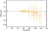Fig. A.1. Value of d2δνs/dn2 per star as a function of Δν. The solid dots indicate the median value, and the vertical lines the spread of d2δνs/dn2 as a function of frequency.

Appendix B: Monte Carlo test for individual models

Here, we investigated the spread obtained in Δν and α following the 5% uncertainty we induced on ν_max and the uncertainties on the individual frequencies as per Ahlborn et al. (2025). For this investigation, we take three models with different values of ν_max, see Fig. B.1. The induced spread on ν_max and the fact that the oscillations are chosen closest to ν_max, means that we select different sets of frequencies. This results in different values of Δν, each with narrow distributions with minimal or no overlap. Hence, the values are precise to roughly < 1%, consistent with observations, though valid for a specific set of frequencies. The values of α are also affected, although the different distributions tend to overlap.

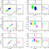Fig. B.1. For three models of one solar mass and solar metallicity, the results of Δν versus νmax (left) and α versus Δν (right) for 5000 perturbations of 5% uncertainty in νmax and the individual frequencies. The different colours indicate different sets of modes (see legend where the n value of the lowest frequency mode of the set is indicated) that are selected to be the ones closest to the perturbed νmax value. The vertical gray dashed line indicates the nominal value of νmax of the respective model. Histograms of the parameters are shown in the top and right panels, respectively, with the same colour code as the main panels.

Appendix C: Mass dependence of α

Here, we provide the α versus Δν values of models with the fits for different masses. The slopes and intercepts of the fits shown in Fig. C.1, have been summarised in Fig. 5.

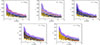Fig. C.1. Curvature, α, as a function of the large frequency separation Δν for RGB stars of solar metallicity, colour-coded by mass. In each panel, the mass that is indicated in the legend is shown on top of all other masses. The red solid and yellow dashed lines are fits to all models of that mass. For the solid line both the slope and the intercept were free parameters, while for the dashed line the slope was kept fixed to the slope of the fit to all models.

All Tables

All Figures

	Fig. 1. Échelle diagram of KIC 2443903 with the degrees of the modes indicated with different colours as per the legend. The curvature, i.e. not straight, vertical orientation of the radial modes is highlighted with the dashed red line.
In the text

	Fig. 2. Curvature (α) as a function of the large frequency separation, with α plotted on a logarithmic scale (left) and a linear scale (right). See the legend for the meanings of the colours.
In the text

	Fig. 3. Curvature (α) as a function of the large-frequency separation (Δν) for RGB stars (left) and CHeB stars (right), colour-coded by mass (top) and metallicity (bottom).
In the text

	Fig. 4. Same as Fig. 3 for results based on our stellar model computations. Note that in the top panels all models have solar metallicity, while in the bottom panels we show only one mass. The latter is the cause of the reduced frequency range of models in panel d.
In the text

Fig. 5. Intercepts (dark grey, left axis) and slopes (pink, right axis) of linear fits in log α versus Δν for RGB models as a function of mass. The points show the mean slope and intercept of fits for 1000 perturbations in which we perturbed both νmax and the individual frequencies within their uncertainties. The vertical bars indicate the spread in the results of these 1000 perturbations. The points connected by a solid line show the results of fits in which both the slope and the intercept were free parameters. The dashed lines connect points for fits with a fixed slope. See text for more details and Fig. C.1 for the fits to the different masses.

In the text

Fig. 6. Curvature (α) as a function of the large frequency separation (Δν) for observations (left) and models (right), split for RGB stars (panels a–d) and CHeB stars (panels e–h), colour-coded by mass (panels a–b and e–f) and metallicity (panels c–d and g–h). The colour code is the same for both the observations and the models. The black lines indicate the RGB and CHeB fits from Fig. 2 and Eq. (7), with the coefficients from Table 1, except for panels c and d, where we use a fit through the selected observed values to account for the dependence of α on mass.

In the text

	Fig. 7. Same as Fig. 6d for uncorrected (top) and surface-corrected frequencies (bottom) using models from Li et al. (2023).
In the text

Fig. 8. Kernels for α (${\underline{K}}_{\alpha }$) as a function of acoustic depth (black and grey) for a 1 M⊙ model with a νmax of about 76 μHz. For comparison, we also show Γ1, the first adiabatic exponent in red, as well as its deviation from 5/3 in the colour code just above it. For comparison, the dashed blue curve shows the radial eigenfunction of the radial mode closest to νmax in arbitrary units.

In the text

Fig. 9. Amplitude (Ag, left) and acoustic depth (τg, centre) as a function of α for direct fits of Eq. (20) to the frequencies of models of 1 M⊙ (blue) and 1.9 M⊙ (orange). The bars indicate the 25th–75th percentiles of the distribution of the results of 5000 perturbations. The tracks evolve from left to right. The positions of the models in the Hertzsprung-Russell diagram are indicated with the dots in the right panel. The lines are the full tracks, shown to guide the eye.

In the text

	Fig. 10. Comparison of α determined via Eq. (3) versus the right-hand side of Eq. (27). The colours and lines have the same meanings as in Fig. 9.
In the text

	Fig. A.1. Value of d2δνs/dn2 per star as a function of Δν. The solid dots indicate the median value, and the vertical lines the spread of d2δνs/dn2 as a function of frequency.
In the text

Fig. B.1. For three models of one solar mass and solar metallicity, the results of Δν versus νmax (left) and α versus Δν (right) for 5000 perturbations of 5% uncertainty in νmax and the individual frequencies. The different colours indicate different sets of modes (see legend where the n value of the lowest frequency mode of the set is indicated) that are selected to be the ones closest to the perturbed νmax value. The vertical gray dashed line indicates the nominal value of νmax of the respective model. Histograms of the parameters are shown in the top and right panels, respectively, with the same colour code as the main panels.

In the text

Fig. C.1. Curvature, α, as a function of the large frequency separation Δν for RGB stars of solar metallicity, colour-coded by mass. In each panel, the mass that is indicated in the legend is shown on top of all other masses. The red solid and yellow dashed lines are fits to all models of that mass. For the solid line both the slope and the intercept were free parameters, while for the dashed line the slope was kept fixed to the slope of the fit to all models.

In the text

References

- Ahlborn, F., Bellinger, E. P., Hekker, S., Basu, S., & Mokrytska, D. 2022, A&A, 668, A98 [NASA ADS] [CrossRef] [EDP Sciences] [Google Scholar]
- Ahlborn, F., Bellinger, E. P., Hekker, S., Basu, S., & Mokrytska, D. 2025, A&A, 693, A274 [NASA ADS] [CrossRef] [EDP Sciences] [Google Scholar]
- Ball, W. H., & Gizon, L. 2014, A&A, 568, A123 [NASA ADS] [CrossRef] [EDP Sciences] [Google Scholar]
- Ball, W. H., Themeßl, N., & Hekker, S. 2018, MNRAS, 478, 4697 [Google Scholar]
- Basu, S. 2016, Liv. Rev. Sol. Phys., 13, 2 [Google Scholar]
- Basu, S., Chaplin, W. J., Elsworth, Y., New, R., & Serenelli, A. M. 2009, ApJ, 699, 1403 [NASA ADS] [CrossRef] [Google Scholar]
- Beck, P. G., Montalban, J., Kallinger, T., et al. 2012, Nature, 481, 55 [Google Scholar]
- Bedding, T. R., Mosser, B., Huber, D., et al. 2011, Nature, 471, 608 [Google Scholar]
- Broomhall, A. M., Miglio, A., Montalbán, J., et al. 2014, MNRAS, 440, 1828 [NASA ADS] [CrossRef] [Google Scholar]
- Buchele, L., Bellinger, E. P., Hekker, S., et al. 2024, ApJ, 961, 198 [Google Scholar]
- Buchele, L., Bellinger, E. P., Hekker, S., & Basu, S. 2025, ApJ, 987, 97 [Google Scholar]
- Choi, J. Y., Espinoza-Rojas, F., Coppée, Q., & Hekker, S. 2025, A&A, 699, A180 [NASA ADS] [CrossRef] [EDP Sciences] [Google Scholar]
- Christensen-Dalsgaard, J., Dappen, W., Ajukov, S. V., et al. 1996, Science, 272, 1286 [Google Scholar]
- Elsworth, Y., Hekker, S., Johnson, J. A., et al. 2019, MNRAS, 489, 4641 [NASA ADS] [CrossRef] [Google Scholar]
- Goldstein, J., & Townsend, R. H. D. 2020, ApJ, 899, 116 [NASA ADS] [CrossRef] [Google Scholar]
- Gough, D. O. 1986, Highlights Astron., 7, 283 [Google Scholar]
- Gough, D. O., & Thompson, M. J. 1991, in Solar Interior and Atmosphere, eds. A. N. Cox, W. C. Livingston, & M. S. Matthews, 519 [Google Scholar]
- Grevesse, N., & Sauval, A. J. 1998, Space Sci. Rev., 85, 161 [Google Scholar]
- Handberg, R., & Lund, M. N. 2014, MNRAS, 445, 2698 [Google Scholar]
- Hekker, S. 2020, Front. Astron. Space Sci., 7, 3 [NASA ADS] [CrossRef] [Google Scholar]
- Hekker, S., Elsworth, Y., De Ridder, J., et al. 2011, A&A, 525, A131 [NASA ADS] [CrossRef] [EDP Sciences] [Google Scholar]
- Hekker, S., Elsworth, Y., & Angelou, G. C. 2018, A&A, 610, A80 [NASA ADS] [CrossRef] [EDP Sciences] [Google Scholar]
- Houdek, G., & Gough, D. O. 2007, MNRAS, 375, 861 [CrossRef] [Google Scholar]
- Jermyn, A. S., Bauer, E. B., Schwab, J., et al. 2023, ApJS, 265, 15 [NASA ADS] [CrossRef] [Google Scholar]
- Kallinger, T., De Ridder, J., Hekker, S., et al. 2014, A&A, 570, A41 [NASA ADS] [CrossRef] [EDP Sciences] [Google Scholar]
- Kjeldsen, H., Bedding, T. R., & Christensen-Dalsgaard, J. 2008, ApJ, 683, L175 [Google Scholar]
- Kosovichev, A. G. 1999, J. Comput. Appl. Math., 109, 1 [NASA ADS] [CrossRef] [Google Scholar]
- Li, Y., Bedding, T. R., Stello, D., et al. 2023, MNRAS, 523, 916 [NASA ADS] [CrossRef] [Google Scholar]
- Lindsay, C. J., Ong, J. M. J., & Basu, S. 2023, ApJ, 950, 19 [CrossRef] [Google Scholar]
- Mazumdar, A., Monteiro, M. J. P. F. G., Ballot, J., et al. 2014, ApJ, 782, 18 [NASA ADS] [CrossRef] [Google Scholar]
- Miglio, A., Montalbán, J., Carrier, F., et al. 2010, A&A, 520, L6 [CrossRef] [EDP Sciences] [Google Scholar]
- Mosser, B., Belkacem, K., Goupil, M. J., et al. 2011, A&A, 525, L9 [CrossRef] [EDP Sciences] [Google Scholar]
- Mosser, B., Goupil, M. J., Belkacem, K., et al. 2012, A&A, 548, A10 [NASA ADS] [CrossRef] [EDP Sciences] [Google Scholar]
- Mosser, B., Michel, E., Belkacem, K., et al. 2013a, A&A, 550, A126 [CrossRef] [EDP Sciences] [Google Scholar]
- Mosser, B., Dziembowski, W. A., Belkacem, K., et al. 2013b, A&A, 559, A137 [CrossRef] [EDP Sciences] [Google Scholar]
- Mosser, B., Benomar, O., Belkacem, K., et al. 2014, A&A, 572, L5 [NASA ADS] [CrossRef] [EDP Sciences] [Google Scholar]
- Mosser, B., Pinçon, C., Belkacem, K., Takata, M., & Vrard, M. 2017, A&A, 600, A1 [NASA ADS] [CrossRef] [EDP Sciences] [Google Scholar]
- Otí Floranes, H., Christensen-Dalsgaard, J., & Thompson, M. J. 2005, MNRAS, 356, 671 [CrossRef] [Google Scholar]
- Paxton, B., Bildsten, L., Dotter, A., et al. 2011, ApJS, 192, 3 [Google Scholar]
- Paxton, B., Cantiello, M., Arras, P., et al. 2013, ApJS, 208, 4 [Google Scholar]
- Paxton, B., Marchant, P., Schwab, J., et al. 2015, ApJS, 220, 15 [Google Scholar]
- Paxton, B., Schwab, J., Bauer, E. B., et al. 2018, ApJS, 234, 34 [NASA ADS] [CrossRef] [Google Scholar]
- Paxton, B., Smolec, R., Schwab, J., et al. 2019, ApJS, 243, 10 [Google Scholar]
- Pinçon, C., Goupil, M. J., & Belkacem, K. 2020, A&A, 634, A68 [Google Scholar]
- Pinsonneault, M. H., Elsworth, Y. P., Tayar, J., et al. 2018, ApJS, 239, 32 [Google Scholar]
- Prša, A., Harmanec, P., Torres, G., et al. 2016, AJ, 152, 41 [Google Scholar]
- Stello, D., Cantiello, M., Fuller, J., et al. 2016, Nature, 529, 364 [Google Scholar]
- Tassoul, M. 1980, ApJS, 43, 469 [Google Scholar]
- Themeßl, N., Kuszlewicz, J. S., García Saravia Ortiz de Montellano, A., & Hekker, S. 2020, in Stars and their Variability Observed from Space, eds. C. Neiner, W. W. Weiss, D. Baade, et al., 287 [Google Scholar]
- Townsend, R. H. D., & Teitler, S. A. 2013, MNRAS, 435, 3406 [Google Scholar]
- Vrard, M., Mosser, B., Barban, C., et al. 2015, A&A, 579, A84 [CrossRef] [EDP Sciences] [Google Scholar]
The value of nmax is not necessarily an integer.
In this work we were only interested in the radial modes; therefore, the dependence of mode degree ℓ has been omitted.
The π/2 factor to convert the sin of Eq. (20) to cos has been absorbed in the phase ϕ.
We note here that when applying this to observations, the surface effect has to be accounted for.