


| Issue |
A&A
Volume 711, July 2026
Euclid Quick Data Release (Q1)
|
|
|---|---|---|
| Article Number | A37 | |
| Number of page(s) | 17 | |
| Section | Catalogs and data | |
| DOI | https://doi.org/10.1051/0004-6361/202556980 | |
| Published online | 30 June 2026 | |
Euclid: Quick Data Release (Q1) – A photometric search for ultracool dwarfs in the Euclid Deep Fields★
1
Instituto de Astrofísica de Canarias, E-38205 La Laguna, Tenerife, Spain
2
Universidad de La Laguna, Dpto. Astrofísica, E-38206 La Laguna, Tenerife, Spain
3
Instituto de Astrofísica de Canarias, E-38205 La Laguna; Universidad de La Laguna, Dpto. Astrofísica, E-38206 La Laguna, Tenerife, Spain
4
Centro de Astrobiología (CAB), CSIC-INTA, ESAC Campus, Camino Bajo del Castillo s/n, 28692 Villanueva de la Cañada, Madrid, Spain
5
Departamento de Inteligencia Artificial, Universidad Nacional de Educación a Distancia (UNED), c/Juan del Rosal 16, E-28040 Madrid, Spain
6
Laboratoire d’Astrophysique de Bordeaux, CNRS and Université de Bordeaux, Allée Geoffroy St. Hilaire, 33165 Pessac, France
7
Institut universitaire de France (IUF), 1 rue Descartes, 75231 PARIS CEDEX 05, France
8
Department of Astronomy & Astrophysics, University of California at San Diego, 9500 Gilman Drive, La Jolla, CA 92093, USA
9
Department of Physics, International University, Ho Chi Minh City, Vietnam
10
Vietnam National University, Ho Chi Minh City, Vietnam
11
Ohio University, Physics & Astronomy Department, 1 Ohio University, Athens, OH 45701, USA
12
International Space University, 1 rue Jean-Dominique Cassini, 67400 Illkirch-Graffenstaden, France
13
Université de Strasbourg, CNRS, Observatoire astronomique de Strasbourg, UMR 7550, 67000 Strasbourg, France
14
Universite Marie et Louis Pasteur, CNRS, Observatoire des Sciences de l’Univers THETA Franche-Comte Bourgogne, Institut UTINAM, Observatoire de Besançon, BP 1615, 25010 Besançon Cedex, France
15
INAF-Osservatorio Astrofisico di Torino, Via Osservatorio 20, 10025 Pino Torinese (TO), Italy
16
Department of Physics, Astronomy and Mathematics, University of Hertfordshire, College Lane, Hatfield AL10 9AB, UK
17
Université Paris-Saclay, CNRS, Institut d’astrophysique spatiale, 91405 Orsay, France
18
ESAC/ESA, Camino Bajo del Castillo, s/n., Urb. Villafranca del Castillo, 28692 Villanueva de la Cañada, Madrid, Spain
19
School of Mathematics and Physics, University of Surrey, Guildford, Surrey GU2 7XH, UK
20
INAF-Osservatorio Astronomico di Brera, Via Brera 28, 20122 Milano, Italy
21
INAF-Osservatorio di Astrofisica e Scienza dello Spazio di Bologna, Via Piero Gobetti 93/3, 40129 Bologna, Italy
22
IFPU, Institute for Fundamental Physics of the Universe, via Beirut 2, 34151 Trieste, Italy
23
INAF-Osservatorio Astronomico di Trieste, Via G. B. Tiepolo 11, 34143 Trieste, Italy
24
INFN, Sezione di Trieste, Via Valerio 2, 34127 Trieste TS, Italy
25
SISSA, International School for Advanced Studies, Via Bonomea 265, 34136 Trieste TS, Italy
26
Dipartimento di Fisica e Astronomia, Università di Bologna, Via Gobetti 93/2, 40129 Bologna, Italy
27
INFN-Sezione di Bologna, Viale Berti Pichat 6/2, 40127 Bologna, Italy
28
INAF-Osservatorio Astronomico di Padova, Via dell’Osservatorio 5, 35122 Padova, Italy
29
Space Science Data Center, Italian Space Agency, via del Politecnico snc, 00133 Roma, Italy
30
Dipartimento di Fisica, Università di Genova, Via Dodecaneso 33, 16146 Genova, Italy
31
INFN-Sezione di Genova, Via Dodecaneso 33, 16146 Genova, Italy
32
Department of Physics “E. Pancini”, University Federico II, Via Cinthia 6, 80126 Napoli, Italy
33
INAF-Osservatorio Astronomico di Capodimonte, Via Moiariello 16, 80131 Napoli, Italy
34
Instituto de Astrofísica e Ciências do Espaço, Universidade do Porto, CAUP, Rua das Estrelas, PT4150-762 Porto, Portugal
35
Faculdade de Ciências da Universidade do Porto, Rua do Campo de Alegre, 4150-007 Porto, Portugal
36
Dipartimento di Fisica, Università degli Studi di Torino, Via P. Giuria 1, 10125 Torino, Italy
37
INFN-Sezione di Torino, Via P. Giuria 1, 10125 Torino, Italy
38
European Space Agency/ESTEC, Keplerlaan 1, 2201 AZ, Noordwijk, The Netherlands
39
Institute Lorentz, Leiden University, Niels Bohrweg 2, 2333 CA, Leiden, The Netherlands
40
Leiden Observatory, Leiden University, Einsteinweg 55, 2333 CC, Leiden, The Netherlands
41
INAF-IASF Milano, Via Alfonso Corti 12, 20133 Milano, Italy
42
Centro de Investigaciones Energéticas, Medioambientales y Tecnológicas (CIEMAT), Avenida Complutense 40, 28040 Madrid, Spain
43
Port d’Informació Científica, Campus UAB, C. Albareda s/n, 08193 Bellaterra (Barcelona), Spain
44
Institute for Theoretical Particle Physics and Cosmology (TTK), RWTH Aachen University, 52056 Aachen, Germany
45
INAF-Osservatorio Astronomico di Roma, Via Frascati 33, 00078 Monteporzio Catone, Italy
46
INFN section of Naples, Via Cinthia 6, 80126 Napoli, Italy
47
Institute for Astronomy, University of Hawaii, 2680 Woodlawn Drive, Honolulu, HI 96822, USA
48
Dipartimento di Fisica e Astronomia “Augusto Righi” – Alma Mater Studiorum Università di Bologna, Viale Berti Pichat 6/2, 40127 Bologna, Italy
49
Institute for Astronomy, University of Edinburgh, Royal Observatory, Blackford Hill, Edinburgh EH9 3HJ, UK
50
Jodrell Bank Centre for Astrophysics, Department of Physics and Astronomy, University of Manchester, Oxford Road, Manchester M13 9PL, UK
51
European Space Agency/ESRIN, Largo Galileo Galilei 1, 00044 Frascati, Roma, Italy
52
Université Claude Bernard Lyon 1, CNRS/IN2P3, IP2I Lyon, UMR 5822, Villeurbanne F-69100, France
53
Institut de Ciències del Cosmos (ICCUB), Universitat de Barcelona (IEEC-UB), Martí i Franquès 1, 08028 Barcelona, Spain
54
Institució Catalana de Recerca i Estudis Avançats (ICREA), Passeig de Lluís Companys 23, 08010 Barcelona, Spain
55
UCB Lyon 1, CNRS/IN2P3, IUF, IP2I Lyon, 4 rue Enrico Fermi, 69622 Villeurbanne, France
56
Mullard Space Science Laboratory, University College London, Holmbury St Mary, Dorking, Surrey RH5 6NT, UK
57
Canada-France-Hawaii Telescope, 65-1238 Mamalahoa Hwy, Kamuela, HI 96743, USA
58
Aix-Marseille Université, CNRS, CNES, LAM, Marseille, France
59
Departamento de Física, Faculdade de Ciências, Universidade de Lisboa, Edifício C8, Campo Grande, PT1749-016 Lisboa, Portugal
60
Instituto de Astrofísica e Ciências do Espaço, Faculdade de Ciências, Universidade de Lisboa, Campo Grande, 1749-016 Lisboa, Portugal
61
Department of Astronomy, University of Geneva, ch. d’Ecogia 16, 1290 Versoix, Switzerland
62
INFN-Padova, Via Marzolo 8, 35131 Padova, Italy
63
Aix-Marseille Université, CNRS/IN2P3, CPPM, Marseille, France
64
INAF-Istituto di Astrofisica e Planetologia Spaziali, via del Fosso del Cavaliere, 100, 00100 Roma, Italy
65
School of Physics, HH Wills Physics Laboratory, University of Bristol, Tyndall Avenue, Bristol BS8 1TL, UK
66
Universitäts-Sternwarte München, Fakultät für Physik, Ludwig-Maximilians-Universität München, Scheinerstr. 1, 81679 München, Germany
67
FRACTAL S.L.N.E., calle Tulipán 2, Portal 13 1A, 28231 Las Rozas de Madrid, Spain
68
Max Planck Institute for Extraterrestrial Physics, Giessenbachstr. 1, 85748 Garching, Germany
69
Institute of Theoretical Astrophysics, University of Oslo, P.O. Box 1029 Blindern, 0315 Oslo, Norway
70
Jet Propulsion Laboratory, California Institute of Technology, 4800 Oak Grove Drive, Pasadena, CA 91109, USA
71
Felix Hormuth Engineering, Goethestr. 17, 69181 Leimen, Germany
72
Technical University of Denmark, Elektrovej 327, 2800 Kgs. Lyngby, Denmark
73
Cosmic Dawn Center (DAWN), Denmark
74
Max-Planck-Institut für Astronomie, Königstuhl 17, 69117 Heidelberg, Germany
75
NASA Goddard Space Flight Center, Greenbelt, MD 20771, USA
76
Department of Physics and Helsinki Institute of Physics, Gustaf Hällströmin katu 2, University of Helsinki, 00014 Helsinki, Finland
77
Université de Genève, Département de Physique Théorique and Centre for Astroparticle Physics, 24 quai Ernest-Ansermet, CH-1211 Genève 4, Switzerland
78
Department of Physics, P.O. Box 64, University of Helsinki, 00014 Helsinki, Finland
79
Helsinki Institute of Physics, Gustaf Hällströmin katu 2, University of Helsinki, 00014 Helsinki, Finland
80
Centre de Calcul de l’IN2P3/CNRS, 21 avenue Pierre de Coubertin, 69627 Villeurbanne Cedex, France
81
Laboratoire d’etude de l’Univers et des phenomenes eXtremes, Observatoire de Paris, Université PSL, Sorbonne Université, CNRS, 92190 Meudon, France
82
SKAO, Jodrell Bank, Lower Withington, Macclesfield SK11 9FT, UK
83
Dipartimento di Fisica “Aldo Pontremoli”, Università degli Studi di Milano, Via Celoria 16, 20133 Milano, Italy
84
INFN-Sezione di Milano, Via Celoria 16, 20133 Milano, Italy
85
Universität Bonn, Argelander-Institut für Astronomie, Auf dem Hügel 71, 53121 Bonn, Germany
86
INFN-Sezione di Roma, Piazzale Aldo Moro, 2 – c/o Dipartimento di Fisica, Edificio G. Marconi, 00185, Roma, Italy
87
Dipartimento di Fisica e Astronomia “Augusto Righi” – Alma Mater Studiorum Università di Bologna, via Piero Gobetti 93/2, 40129 Bologna, Italy
88
Department of Physics, Institute for Computational Cosmology, Durham University, South Road, Durham DH1 3LE, UK
89
Université Paris Cité, CNRS, Astroparticule et Cosmologie, 75013 Paris, France
90
CNRS-UCB International Research Laboratory, Centre Pierre Binétruy, IRL2007, CPB-IN2P3, Berkeley, USA
91
Institut d’Astrophysique de Paris, 98bis Boulevard Arago, 75014 Paris, France
92
Institut d’Astrophysique de Paris, UMR 7095, CNRS, and Sorbonne Université, 98 bis boulevard Arago, 75014 Paris, France
93
Institute of Physics, Laboratory of Astrophysics, Ecole Polytechnique Fédérale de Lausanne (EPFL), Observatoire de Sauverny, 1290 Versoix, Switzerland
94
Aurora Technology for European Space Agency (ESA), Camino bajo del Castillo, s/n, Urbanizacion Villafranca del Castillo, Villanueva de la Cañada, 28692 Madrid, Spain
95
Institut de Física d’Altes Energies (IFAE), The Barcelona Institute of Science and Technology, Campus UAB, 08193 Bellaterra (Barcelona), Spain
96
DARK, Niels Bohr Institute, University of Copenhagen, Jagtvej 155, 2200 Copenhagen, Denmark
97
Waterloo Centre for Astrophysics, University of Waterloo, Waterloo, Ontario N2L 3G1, Canada
98
Department of Physics and Astronomy, University of Waterloo, Waterloo, Ontario N2L 3G1, Canada
99
Perimeter Institute for Theoretical Physics, Waterloo, Ontario N2L 2Y5, Canada
100
Université Paris-Saclay, Université Paris Cité, CEA, CNRS, AIM, 91191 Gif-sur-Yvette, France
101
Centre National d’Etudes Spatiales – Centre spatial de Toulouse, 18 avenue Edouard Belin, 31401 Toulouse Cedex 9, France
102
Institute of Space Science, Str. Atomistilor, nr. 409 Măgurele, Ilfov 077125, Romania
103
Consejo Superior de Investigaciones Cientificas, Calle Serrano 117, 28006 Madrid, Spain
104
Dipartimento di Fisica e Astronomia “G. Galilei”, Università di Padova, Via Marzolo 8, 35131 Padova, Italy
105
Institut für Theoretische Physik, University of Heidelberg, Philosophenweg 16, 69120 Heidelberg, Germany
106
Institut de Recherche en Astrophysique et Planétologie (IRAP), Université de Toulouse, CNRS, UPS, CNES, 14 Av. Edouard Belin, 31400 Toulouse, France
107
Université St Joseph; Faculty of Sciences, Beirut, Lebanon
108
Departamento de Física, FCFM, Universidad de Chile, Blanco Encalada 2008, Santiago, Chile
109
Institut d’Estudis Espacials de Catalunya (IEEC), Edifici RDIT, Campus UPC, 08860 Castelldefels, Barcelona, Spain
110
Satlantis, University Science Park, Sede Bld 48940, Leioa-Bilbao, Spain
111
Institute of Space Sciences (ICE, CSIC), Campus UAB, Carrer de Can Magrans, s/n, 08193 Barcelona, Spain
112
Instituto de Astrofísica e Ciências do Espaço, Faculdade de Ciências, Universidade de Lisboa, Tapada da Ajuda, 1349-018 Lisboa, Portugal
113
Cosmic Dawn Center (DAWN)
114
Niels Bohr Institute, University of Copenhagen, Jagtvej 128, 2200 Copenhagen, Denmark
115
Universidad Politécnica de Cartagena, Departamento de Electrónica y Tecnología de Computadoras, Plaza del Hospital 1, 30202 Cartagena, Spain
116
Centre for Information Technology, University of Groningen, P.O. Box 11044, 9700 CA, Groningen, The Netherlands
117
INFN-Bologna, Via Irnerio 46, 40126 Bologna, Italy
118
Kapteyn Astronomical Institute, University of Groningen, PO Box 800, 9700 AV, Groningen, The Netherlands
119
Infrared Processing and Analysis Center, California Institute of Technology, Pasadena, CA 91125, USA
120
ICL, Junia, Université Catholique de Lille, LITL, 59000 Lille, France
★★ Corresponding author: This email address is being protected from spambots. You need JavaScript enabled to view it.
Received:
25
August
2025
Accepted:
1
December
2025
Abstract
We present a catalogue of 5306 new ultracool dwarf (UCD) candidates in the three Euclid Deep Fields in the Q1 data release. They range from late M to late T dwarfs, and include 1200 L and T dwarfs. A total of 546 objects have been spectroscopically confirmed, including 329 L dwarfs and 26 T dwarfs. We also provide empirical Euclid colours as a function of spectral type. Our UCD selection criteria are based only on colour (IE − YE > 2.5). The combined requirement for optical detection and a stringent signal-to-noise ratio threshold ensure a high purity of the sample, but at the expense of completeness, especially for T dwarfs. The detections range from magnitudes 19 and 24 in the near-infrared bands, and extend down to 26 in the optical band. We discuss Euclid’s capability to identify UCD candidates based on its photometric passbands. The average surface density of detected UCDs on the sky is approximately 100 objects per deg2, including 20 L and T dwarfs per deg2. This leads to an expectation of at least 1.4 million UCDs in the final data release of the Euclid Wide Survey, including at least 300 000 L dwarfs, and more than 2600 T dwarfs, using the strict selection criteria from this work.
Key words: catalogs / brown dwarfs
Publisher note: the very beginning of the author list was corrected on 10 July 2026.
This paper is published on behalf of the Euclid Consortium.
© The Authors 2026
 Open Access article, published by EDP Sciences, under the terms of the Creative Commons Attribution License (https://creativecommons.org/licenses/by/4.0), which permits unrestricted use, distribution, and reproduction in any medium, provided the original work is properly cited.
This article is published in open access under the Subscribe to Open model. This email address is being protected from spambots. You need JavaScript enabled to view it. to support open access publication.
1. Introduction
Ultracool dwarfs (UCDs), comprising the lowest-mass stars, brown dwarfs, and free-floating planetary-mass objects, represent a continuum of properties linking stellar and planetary physics. Their formation mechanisms remain vigorously debated: with questions surrounding whether they form like stars, via the gravitational collapse and fragmentation of molecular clouds, or like planets, through disc instabilities or core accretion followed by ejection (Whitworth 2018; Miret-Roig et al. 2022; Palau et al. 2024). Despite their intrinsic faintness, they are abundant, making up a significant fraction of the Galaxy’s population. Yet, their census remains incomplete, particularly at the faint and metal-poor ends. Building large, homogeneous catalogues and developing robust photometric and astrometric diagnostics to distinguish UCDs from background contaminants are therefore crucial steps towards constraining their formation pathways. In turn, this will shed light on the broader processes of star and planet formation, helping to advance our understanding of the lowest-mass end of the initial mass function.
The advent of major wide area imaging and spectroscopic surveys from the ground and from space, at optical and infrared wavelengths, has enabled the discovery of hundreds of UCDs. Traditionally, these faint ultracool objects are first identified by photometric selection criteria using large survey catalogues (e.g. Sloan Digital Sky Survey (SDSS; York et al. 2000), Two-Micron All-Sky Survey (2MASS; Cutri et al. 2003; Skrutskie et al. 2006), Deep Near Infrared Survey of the Southern Sky (DENIS; Epchtein et al. 1997), UKIRT Infrared Deep Sky Survey (UKIDSS; Lawrence et al. 2007), Wide-field Infrared Survey Explorer (WISE; Wright et al. 2010), VISTA Hemisphere Survey (VHS; McMahon et al. 2013), Panoramic Survey Telescope and Rapid Response System (Pan-STARRS; Chambers et al. 2016), and the Dark Energy Survey (DES; Abbott et al. 2021)), and later confirmed spectroscopically (e.g. Kirkpatrick et al. 1999, 2000; Luhman 2014; Martín et al. 1999, 2010; Reylé 2018). For example, dal Ponte et al. (2023) extended the catalogue of Carnero Rosell et al. (2019) and identified almost 20 000 UCD candidates brighter than z ≤ 23 in DES. On the other hand, the Ultracool Sheet1 (Best et al. 2024) – the growing literature compilation of confirmed UCDs and imaged planets – contains more than 4000 objects, as of December 2024.
The Euclid space mission (Euclid Collaboration: Mellier et al. 2025) is a wide-field space telescope equipped with high-precision optical and near-infrared imaging and slitless spectroscopy. It is designed to observe distant galaxies to explore the composition and evolution of the dark Universe. At the same time, its high sensitivity and wide coverage enable the identification of thousands of new UCDs. This is made possible primarily by its sensitive Near-Infrared Photometer and Spectrometer (NISP, Euclid Collaboration: Jahnke et al. 2025), which observes wavelengths that are otherwise partially obscured by Earth’s atmosphere, such as water absorption bands. This spectral range also reveals key molecules in UCD atmospheres, such as methane. Euclid’s high sensitivity makes it possible to detect fainter objects than in previous wide-field surveys. The depth provided by the Q1 data allows us to probe about 3 magnitudes deeper at optical and near-infrared wavelengths than previous ground-based surveys. The limiting sensitivity in the optical is 26.7 (Euclid Collaboration: Mellier et al. 2025), and 24.4 (5σ point source) in the near-infrared, and this enables the detection of faint, free-floating planetary-mass objects. For example, the first scientific results of Euclid were derived from the Early Release Observations (ERO; Cuillandre et al. 2025), which included the photometric identification of new UCDs in the Sigma Orionis open cluster (Martín et al. 2025) and the LDN 1495 region of the Taurus molecular clouds (Bouy et al. 2025). Owing to the young age of these regions, such objects have likely planetary masses, down to a few Jupiter masses. Upon completion of the wide (Euclid Wide Survey, EWS) and deep (Euclid Deep Survey, EDS) surveys that will take over 5 years, it has been predicted that Euclid will have detected the largest ever number of UCDs, most of which will be present only in the near-infrared images (Solano et al. 2021). The resulting large catalogue will help us better understand the populations of UCDs and their formation scenarios, and help us refine the models of their interiors and complex atmospheres.
This work presents the first study to assess the potential of Euclid’s passbands to identify UCDs in its observations. By exploring the UCD parameter space using photometric data from the Euclid’s first Quick Data Release, Q1 (Euclid Quick Release Q1 2025), we evaluated its capability to detect UCDs on a large scale, comparing it with the spectroscopic search and analysis from Dominguez-Tagle et al. (2025) and Mohandasan et al. (2025). Our goal was to understand both the strengths and limitations of the photometric data in identifying UCDs. Since the depth of the Q1 matches that of the planned EWS, this study provides a direct estimate of the expected UCD yield in the final EWS at the end of the mission – representing a crucial step towards understanding the final survey’s potential.
To ensure high reliability, we searched for UCDs detected in both near-infrared and optical bands. The resulting catalogue has a relatively low contamination rate at the cost of completeness. Fainter detections in the near-infrared EDF observations will be examined in a follow-up study and in future repeated observations, which will probe even deeper.
This paper is structured as follows. In Sect. 2, we present the Euclid’s Q1 data along with known UCDs from the literature, which are included in this dataset and used as benchmarks. We describe the extraction of point sources from the Euclid catalogue in Sect. 3. Section 4 details the selection process for candidate UCDs in our dataset. In Sect. 6, we examine the properties of our candidate UCD catalogue, their spectral types and empirical colours, the catalogue’s limitations, and the expected number of UCD detections in the future Euclid observations. Finally, we draw our conclusions in Sect. 7. We provide lists of spectroscopically confirmed benchmark sources and T dwarfs, as well as our main photometric UCD candidates, in Appendix A.
2. Data
In this paper we utilise the three catalogues of the EDFs from the Q1 data release. They cover a total area of 63 deg2, distributed approximately as follows (see Euclid Collaboration: Aussel et al. 2026): EDF Fornax (EDF-F), 12 deg2; EDF North (EDF-N), 23 deg2; and EDF South (EDF-S), 28 deg2. This data release includes only the first visit of these fields, but they will be continuously observed many times during the lifetime of the mission, which will deepen the detection limit by another 2 magnitudes.
We exploited the merged catalogue (MER) that consists of photometric and morphological information of 39 million objects detected in all three fields. They were observed with two instruments, VIS (magnitude IE, Euclid Collaboration: Cropper et al. 2025), with one wide visible filter, and NISP, with three photometric filters that give magnitudes YE, JE, and HE. All four filters are broader than the standard ground-based photometric passbands; their widths range from 0.3 to 0.56 μm. Together, they cover wavelengths from about 0.5 to 2 μm, with almost no gaps. The passbands2 have the following central wavelengths: 0.67 μm in IE; 1.08 μm in YE; 1.37 μm in JE; and 1.77 μm in HE (Euclid Collaboration: Schirmer et al. 2022).
The MER catalogue provides magnitudes computed in a few different ways. In this work, we adopted aperture photometry computed within twice the full width at half maximum (FWHM), with magnitudes expressed in the AB photometric system. Our choice of flux type from the MER catalogue follows the work of Mohandasan et al. (2025), where the authors discuss the optimal flux measurement for point-like sources, and compare the magnitudes with ground-based photometry.
2.1. Reference UCDs in Euclid fields
Anticipating the first Euclid observations, Zhang et al. (2024) analysed the existing optical and infrared photometric catalogues to search for the UCDs in the EDFs. They used Pan-STARRS release 1, 2MASS, and the AllWISE survey (Cutri et al. 2021) to search for late M, L, and T dwarfs. Their photometric selection criteria were based on the work of Carnero Rosell et al. (2019), but generalised and less strict. They found 360 M, 152 L, and three T candidate dwarfs in the three EDFs. From this sample they selected eight UCD candidates of different spectral types and obtained spectra with EMIR the Espectrógrafo Multiobjeto Infra-Rojo (EMIR; Garzón et al. 2022) at the Gran Telescopio Canarias (GTC), and the Very Large Telescope (VLT)/Xshooter, which confirm their UCD nature.
3. Selection of point sources
The most common objects in Euclid’s catalogue are extragalactic. They are clearly extended when they are close enough, although they appear point-like when very distant. Fortunately, in our parameter space of choice, there is negligible overlap between the point-like galaxies and stars, and especially substellar objects (see Sect. 6.2). To isolate the point-like sources, we performed a series of simple morphology and data quality filters using measurements already available3 in the Q1 tables. Our criteria were stringent, leaving out some marginal objects, such as young UCDs, which might appear extended due to a potential circumsubstellar disc and infalling material. Our goal was to produce a catalogue that is as free of contaminants as possible, rather than aiming for completeness. Our selection was defined with the help of the benchmark ultracool objects from Table A.1.
The most restrictive requirements were applied to the morphology of the sources, since most of the objects in Euclid’s catalogue are galaxies. Due to POINT_LIKE_PROB (probability between 0 and 1 that the source is point-like) being available only for a subset of sources, due to the strong priority placed on purity in the MER catalogue (Euclid Collaboration: Romelli et al. 2026), we designed our own filters that are a little less restrictive and reach fainter magnitudes. To isolate point-like objects, we used the ELLIPTICITY and MUMAX_MINUS_MAG parameters. ELLIPTICITY is defined as 1 − B/A, where A and B are the semi-major and semi-minor axes of an elliptical object, respectively, and are computed directly by SourceExtractor (Bertin & Arnouts 1996). MUMAX_MINUS_MAG is a proxy for the better-known SPREAD_MODEL parameter (Mohr et al. 2012; Desai et al. 2012; Bouy et al. 2013), and is directly used for star–galaxy separation. It is defined as the difference between the peak surface brightness above the background (MUMAX in mag arcsec−2) and the magnitude (Euclid Collaboration: Romelli et al. 2026). Essentially, it compares the concentration of the light at the peak and the total magnitude. This difference distinguishes extended and point sources very efficiently, as is demonstrated in Fig. 1. We limited this parameter to values between −3.25 and −2.65 mag arcsec−2, and ELLIPTICITY to < 0.2.
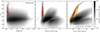 |
Fig. 1. Morphological filters differentiate between extended sources and point sources. The filtering criteria (red lines for ELLIPTICITY and MUMAX_MINUS_MAG) are based on the benchmark UCDs (red dots; Zhang et al. 2024). Grey dots are sources from the entire Euclid catalogue. The right panel shows that while KRON_RADIUS is not used in the procedure, it correlates well with luminosity for the point sources. |
The distribution of FWHM ranges from about 1 1 to 1
 5 for the majority of sources. Because one of the benchmarks is an outlier in this parameter (its det_quality_flag is 386, which means bad data quality) and lies beyond that limit, we formally introduced a
  filter to exclude it. This filter removed fewer than 1% of sources from the entire sample.
Saturated, blended, and contaminated sources, and those with similar problems, were excluded with the DET_QUALITY_FLAG smaller than 3. To limit ourselves only to the measurements of high quality, we eliminated all catalogue entries with a signal-to-noise ratio (S/N; defined as flux/flux error) of less than 4. This is the most restrictive selection criterion, which consequently shifts the completeness by 1–1.5 mag, and the limiting magnitude by several magnitudes, as is demonstrated in Fig. 2. The completeness limit in our resulting point-source catalogue, after all applied cuts, is 23.5 for the near-infrared bands and 24.5 in the visible, as is shown in Fig. 3. We imposed such a strict constraint in order to produce as clean a sample as possible, at the expense of the fainter sources, which will be explored in a follow-up work. We applied this filtering only to the IE, YE, and HE bands that are essential for our UCD science. The JE data remained unfiltered, because our UCD selection criteria, described below, are not based on the JE magnitude. This means that some of our sources might have bad pixels in the JE band, but since this magnitude is not used, it does not affect our results.
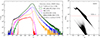 |
Fig. 2. Magnitude distributions and signal-to-noise characteristics of the point-source catalogue. Left: Magnitude distributions for each point-source selection filter (we do not plot the FWHM filter). The most limiting is the S/N requirement that raises the completeness and detection limits to ensure a high quality of the point-source catalogue. Right: Signal-to-noise ratio as a function of luminosity. A cut at S/N = 4 is imposed. |
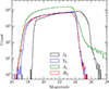 |
Fig. 3. Magnitude distributions in the point-source catalogue. Completeness limits are approximately 23.5 for the NISP bands and 24.5 for VIS. The filtering procedure was not applied to the JE band, since it was not used in the candidate selection from the colour-colour diagram. |
We present the set of filters that we use in Table 1. This simple but effective filtering resulted in a catalogue of 688 957 point sources, representing just under 2% of the initial sample.
Filters applied to isolate point sources.
We estimated magnitude and colour error bars for the point source catalogue by sampling 1000 flux values from a normal distribution centred on the measured flux, using the flux error as the standard deviation. These sampled fluxes were then converted to magnitudes, and the 16th and 84th percentiles of the resulting distribution were taken as the lower and upper bounds of the uncertainty.
3.1. Extinction estimation
We found an apparent relative offset between the EDF-N and the two southern fields in our IE − YE versus YE − HE diagrams. This is shown, for example, in Fig. 4, where we plot data from EDF-N and EDF-S. The difference is particularly noticeable in the densest regions, representing solar-like stars. The relative offsets of EDF-N with respect to EDF-S are 0.04 in IE − YE and 0.02 in YE − HE. This might be coming from differences in interstellar extinction. While the EDFs were carefully selected to be extinction-free, the average estimated4E(B − V) in the northern field (0.056) is more than 3 times higher than in EDF-S (0.017). This corresponds to median extinction values of AIE = 0.13, AYE = 0.06, and AHE = 0.03 in EDF-N, and AIE = 0.08, AYE = 0.02, and AHE = 0.009 in EDF-S. They are typically 2–3-times larger in EDF-N, depending on the wavelength. This difference could produce the relative offsets that we detected in the data.
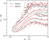 |
Fig. 4. Euclid colour-colour diagram. The offset between EDF-N and EDF-S is most prominent in the solar-like region at 0.1 < IE − YE < 0.4. |
However, the reddening values are upper limits, and the actual values for the UCDs, which are very close to us, are smaller. Additionally, the offsets between EDF-S and EDF-N are much smaller than the typical error bars for individual UCDs (±0.12 and ±0.06, respectively). For this reason, we did not apply any corrections.
4. A catalogue of photometric UCD candidates
We visualise our point-source catalogue in a colour-colour diagram in Fig. 5. We followed Martín et al. (2025) and chose a combination of IE − YE and YE − HE that brings out the UCDs most clearly. The use of the optical band helped us to construct a high-quality catalogue of UCDs with minimal contamination, but at the expense of completeness, especially for the reddest objects (T dwarfs). We provide more details about this topic in Sect. 6.2.
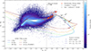 |
Fig. 5. Bluebottle diagram of point sources. The central sequence starts with white dwarfs below IE − YE < 0, continues with stars, and ends in the cool tip with UCDs at IE − YE ≳ 2.5. Their nature is confirmed with the benchmark UCDs from Zhang et al. (2024). We overplotted both the new photometric candidate T dwarfs from this work (symbols with error bars), and those that were spectroscopically confirmed (open circles), as listed in Table A.2. ATMO models (Phillips et al. 2020) indicate the UCD parameter space, while the PARSEC model traces main sequence and evolved stars with redder YE − HE. |
The data in our chosen parameter space form a shape that resembles a bluebottle5 with the main body, sail, and tentacles. Therefore, we have named this colour-colour plot the ‘bluebottle’ diagram. Its central sequence starts with white dwarfs below IE − YE < 0, continues with stars, and ends in the cool tip with UCDs at IE − YE ⪆ 2.5. To identify the region occupied by UCDs in Fig. 5, we overplotted the known UCDs from Zhang et al. (2024) that have been spectroscopically confirmed by Dominguez-Tagle et al. (2025) using Euclid spectra. For clarity, Fig. 6 shows an expanded area of the bluebottle diagram, including the cool tip and the spectroscopically confirmed UCDs. They perfectly overlap with the bluebottle, and demonstrate that this parameter space encompasses UCDs from late M dwarfs down to late T dwarfs.
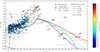 |
Fig. 6. Zoom into the cool tip of the bluebottle diagram showing the benchmark objects (coloured dots with error bars). The spectral types are from Dominguez-Tagle et al. (2025). We overplotted typical positions for each spectral type from the curve fits (red squares) and ATMO models for a range of ages. |
We used the spectroscopically confirmed UCDs as a guide in our candidate UCD selection. Figure 6 shows that the typical IE − YE colour of the M8 dwarfs is about 2.5. We therefore used the IE − YE > 2.5 criterion to select the photometric UCD candidates in this work. Such a cut isolated 5306 objects, with the reddest IE − YE colours ranging between 2.5 (∼M8) and 5.0 (late T dwarfs). According to their colour distribution, shown in Fig. 7, we expect to find about 1200 L dwarfs with IE − YE > 2.9. Additionally, we report a list of 13 candidate T dwarfs. One of them has been previously identified (Zhang et al. 2024), and the rest are new. Seven of them have been spectroscopically confirmed using Euclid spectra, as is shown in figure 7 in Dominguez-Tagle et al. (2025). These objects are listed in Table A.2, as well as in the main UCD catalogue. The number of T dwarfs is relatively small. This is because they are intrinsically faint, and due to our selection biases, discussed in more detail in Sect. 6.2. In Table A.3 we provide the main result of this work, a list of 5306 photometric UCD candidates. Of these, 546 have been assigned spectral type following the procedure from Dominguez-Tagle et al. (2025).
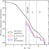 |
Fig. 7. Reverse cumulative distribution, showing how many objects are redder than the selected colour. There are 5306 objects redder than 2.5, which correspond to late M dwarfs, and 1200 objects redder than 2.9, which roughly correspond to L0 dwarfs. The red curve corresponds to objects whose spectra exhibit UCD features, whereas the blue line corresponds to objects with assigned spectral types. |
The ATMO models in Fig. 8 predict that early Y dwarfs are expected to be found in the horizontal band below the main bluebottle body, with YE − HE colours roughly between −1.5 and −0.5. A typical IE − YE colour of a Y0 dwarf is around 5, while we can expect objects with masses below ∼20 MJup at IE − YE ≃ 2.5. There are a number of objects in this region in the figure. We manually inspected their spectra (although they are not available for all objects) and could not confirm any Y dwarfs. On the other hand, based on the colours of known Y dwarfs (e.g. Kirkpatrick et al. 2024), we expect Y dwarfs to have IE − YE colours that are even redder than T dwarfs, and YE − HE colours that are bluer than T dwarfs, i.e. we expect them to extend the T dwarf sequence towards the bottom right in the bluebottle diagram. There are no objects in our catalogue with such colours.
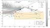 |
Fig. 8. Bluebottle diagram focused on the UCDs. Models predict that early Y dwarfs are located in a horizontal band below the main bluebottle body. While there are many photometric candidates found there, none of them have been spectroscopically confirmed. We manually inspected the available spectra of the objects below the black line and found that most of them are not consistent with UCDs (black crosses). Apart from the T dwarfs, only seven other objects show UCD (or stellar) spectra. |
The absence of detected Y dwarfs is likely due to our strict filtering criteria. Namely, the absolute IE magnitude of an Y0 object at 10 Myr is around 26.2, which is already beyond the completeness limit (see Fig. 3). Conversely, Dominguez-Tagle et al. (2025) performed an independent search for UCDs in the entire Euclid spectral database, and did not find any Y dwarfs. This might be due to the fact that in the Q1 data release, spectra are only available for HE < 22.5 objects. This will change in the forthcoming data releases. In the future, a development of search criteria based only on NISP, supplemented with the ground-based photometry, might yield a detection of Y dwarfs in Euclid, as is discussed in Sect. 6.2.
5. A catalogue of spectroscopically confirmed UCDs
To assess the nature of the selected candidates, we examined the available spectra for these objects (Euclid Collaboration: Jahnke et al. 2025; Euclid Collaboration: Polenta et al. 2026). Out of 5306 candidates, 4682 have spectra in the Euclid Q1 release (almost 90%). We conducted both a visual spectroscopic analysis and a comparison with the template library, as is described below.
5.1. Manual tagging
Manual tagging was done in the following way. As a first step, we filtered out spectra for which more than 20% of flux points have QUALITY < 0.2, as well as spectra with a mean quality below 0.5. This removed 255 objects from further consideration. To identify additional outliers, we computed the Mahalanobis distance, M (Bishop 2006), selecting spectra with M > 30, which eliminated another 210 objects. These 465 outliers are labeled with ‘O’ in Table A.3.
While these criteria are to some extent subjective, they are necessary to exclude severely degraded or noisy spectra that would hinder further analysis. Visual inspection of the flagged outliers revealed 16 objects that exhibit features characteristic of the UCD spectra, despite being partially corrupted.
To emphasise the spectral morphology, we removed local spikes and applied cubic spline smoothing (full details of the denoising procedure will be presented in a forthcoming publication). The cleaned spectra were then used in the analysis.
We performed a visual comparison of each denoised spectrum against a set of spectral type templates (Burgasser 2014; Burgasser & Splat Development Team 2017). Based on similarity to the templates and the presence of spectral features typical for UCDs in the Euclid NISP red-grism wavelength range (the shape of the H2O absorption bands starting from 1.33 μm, K I doublet at 1.25 μm, H band continuum shape around 1.6 μm), we assigned each spectrum to one of the following classes:
-
C1: Spectra that clearly match UCD templates;
-
C2: Spectra that exhibit some UCD features but do not match any template closely;
-
C3: Spectra that contain a visible signal but lack UCD-specific features;
-
C4: Spectra that are too noisy or corrupted to be classified.
This information is available in Table A.3. There are 496 objects in the C1 category, and 615 in C2. It is possible that many more UCDs are present in our photometric candidate list, but their spectra are currently too noisy or unavailable. In the future, once repeated observations of the EDFs become available, we expect to confirm many more additional candidates. Figure 9 shows that nearly all objects brighter than IE = 22 belong to the C1 class, and that we detected objects with some UCD features (class C2) nearly down to the IE detection limit. The contamination rate is negligible for IE < 22, and likely remains low until IE = 24 where extragalactic objects start to dominate, as is shown in Fig. 1. A contamination estimate based on the number of objects classified into classes C1, C2, and C3 shows that the contamination rate, defined as NC3/NC1 + C2 + C3, where NC3 and NC1 + C2 + C3 are the numbers of objects in these classes, is 67%, consistent with the sharp increase seen at the faint end in Fig. 1. This is, however, a conservative estimate, as the classification into C1-C4 groups was performed manually, and some spectra assigned to the C3 class may still correspond to UCDs whose spectra are simply too heavily degraded for their nature to be confirmed.
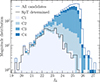 |
Fig. 9. Magnitude distribution of the candidate UCDs with spectra (stacked histogram). Spectral types could be determined for 50% of the entire sample, limited by the S/N of the spectra. While spectral typing is limited at low S/N, spectroscopic confirmation is still possible nearly down to the VIS detection limit. |
5.2. Spectral typing
We considered objects from categories C1 and C2 for spectral classification. This was done by a comparison with the SpeX standard templates (Burgasser 2014; Burgasser & Splat Development Team 2017). We used two different methods, which are described in Dominguez-Tagle et al. (2025). The first method used χ2 minimisation over the full wavelength range. The second one was based on minimising the residual from the difference between the spectra and the standard templates over four wavelength ranges defined by the NISP wavelength range and the telluric absorption bands (i.e. only present in the templates). The spectral type (SpT) was obtained after weighting each method by the quality of the spectrum (see Dominguez-Tagle et al. 2025 for further details). The typical uncertainty of the SpT is ±1 subtype. A colon ‘:’ was added to the spectral subtypes with larger uncertainty, and a ‘p’ for peculiar spectra. Objects with very low S/N were not classified.
In total, 546 spectra had sufficient quality to allow for a reliable determination of spectral types beyond M7. A total of 26 of them are T dwarfs, 329 are L dwarfs, and the rest are late M dwarfs. This means that 10% of our UCD candidates are spectroscopically confirmed and have their SpT determined. The remaining objects from the C1 and C2 groups exhibit some spectral features consistent with UCD classification, for example the water drop at ∼1.35 microns, but the data quality is too limited for definitive spectral typing. We include spectral types in Table A.3.
A comparison with Dominguez-Tagle et al. (2025), who published the SpT of 178 UCDs, reveals 27 objects with SpT that are not in our candidate list. Six of them were found by the spectral index search described in that paper. The remaining 21 are confirmed candidates from Zhang et al. (2024). A close inspection shows that these 21 objects do not meet our point-source and quality requirements (mostly due to low S/N; Sect. 3) or have IE − YE < 2.5. This comparison highlights the importance of conducting both photometric and spectroscopic searches independently, particularly because the latter led to the discovery of five T dwarfs that were not identified through photometry alone (Dominguez-Tagle et al. 2025).
6. Discussion
In this section, we describe the photometric properties of UCDs that have their spectral type determined (Sect. 6.1). Then, we address the contamination rate and the detection limitations of the sample in Sect. 6.2, and the prospects for detecting metal-poor UCDs in Sect. 6.3, compare the dataset with the UCD candidates from the literature (Sect. 6.4), and end with the estimated numbers of future UCD detections in the EDS and EWS, based on the results of this work.
6.1. Empirical photometric sequence
We determined the typical Euclid colours for each UCD spectral type and compared them with the ATMO models used in this work (Phillips et al. 2020). Although our catalogue does not contain any widely studied brown dwarf, its large size allowed us to rely on statistical analysis for late M and L objects. We applied the same analysis to the T dwarfs as well, but the results were less robust due to their scarcity.
Figure 10 shows the relations between the spectral types and the colours. The IE − JE relation is well behaved, which is important since UCDs are brightest in the JE band. Although IE − JE would thus be a preferable selection criterion to IE − YE, the main limitation remains the inclusion of the optical band. For consistency with Martín et al. (2025), we therefore retain IE − YE.
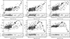 |
Fig. 10. Typical colours for each spectral type. Black dots represent individual objects, crosses mark objects rejected during the sigma-clipping fitting, and open circles indicate objects excluded from the fit due to suspected variability. The black line shows a polynomial fit to the relation. The grey area in the O − C plots represents the standard deviation of the residuals. |
Some spectral types exhibit greater scatter in colour than others. The spread is particularly pronounced for L6–T2 objects, especially in the NISP colours (YE − JE, YE − HE, and JE − HE). This increased scatter is consistent with the known variability during the L–T transition, which is attributed to changes in cloud opacity at near-infrared wavelengths (Radigan et al. 2014; Radigan 2014). Consequently, we observed a discrepancy between the data and the ATMO models in Fig. 6 for late L and early T dwarfs. For this reason, we excluded L6–T2 objects with YE − HE < 0.8 from this analysis, as Fig. 6 indicates that their typical YE − HE colour is greater than 0.9. Additionally, we excluded a small number of photometric outliers whose colours differ by more than 1 magnitude from the typical values of objects with similar spectral types, despite using a sigma-clipping approach in the fit. We provide more detail about this discrepancy in Sect. 6.2.
We fitted a polynomial to each spectral type-colour relation, where spectral types were encoded numerically (e.g. 70 for L0, 75 for L5, 80 for T0, etc.). The order of the polynomial varies depending on the colour, selected to best capture the shape of the relation while avoiding overfitting. To reduce edge artefacts commonly introduced by polynomial fitting, we included a small number of M5 and M6 objects at the lower end of the spectral type range.
Using these polynomial fits, shown in Fig. 10, we derived a typical colour for each spectral type, as is listed in Table 2. The resulting IE − YE versus YE − HE relation aligns well with the bluebottle diagram up to the tip of the sequence (IE − YE ∼ 3.4), but begins to break down for T dwarfs. This discrepancy is likely due to the limited number of T dwarfs in the current dataset, and we expect it to improve with future Euclid data releases.
Empirical Euclid colours for different spectral types.
6.2. Limitations and contamination of the catalogue
Here we discuss the detection limits of the instruments, the quality of the sample, and the contamination of the UCD catalogue with evolved stars and extragalactic objects. The most discriminating parameter in our search for UCDs was the IE − YE colour, which is based on the measurements of two different instruments. Their sensitivities differ: the NISP instrument detects objects with magnitudes between 19 and 24; and the VIS range is broader and extends about 2 magnitudes deeper in our point source catalogue (Fig. 11). Since the UCDs are very red (e.g. the T dwarfs can surpass IE − YE = 4.5), their luminosities in the optical are low. For example, a T dwarf with YE = 24 would be fainter than IE = 28. For this reason, our catalogue of UCD candidates only contains NISP sources brighter than YE ≃ 22.5. The advantage of this limitation is the higher quality of the sample and a higher percentage of objects for which good-quality spectroscopy is available.
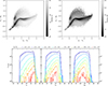 |
Fig. 11. Completeness for the colour bins in the bluebottle diagram. Despite its very high sensitivity, VIS is the most limiting instrument for the detection of UCDs in Euclid. The top panels show a group of bright objects at ≈(0, 0), which are quasars. |
We left the photometric selection of the faint NISP sources for our follow-up work. On the other hand, Dominguez-Tagle et al. (2025) complemented our current catalogue with a spectroscopic search for UCDs, which is not limited by the VIS instrument. They searched for substellar objects in the entire spectroscopic database in Euclid, and found 27 UCD spectra of objects that are not in our candidate list because they did not meet our filtering criteria, mostly due to a poor S/N. Similarly, Mohandasan et al. (2025) used spectroscopic templates to search for UCDs and confirmed 33 new objects, ranging from spectral types M7 to T1.
As is discussed in Sect. 6.1, approximately 75% of objects in the L–T transition region exhibit colours that deviate significantly from those expected for their spectral types, particularly in the near-infrared. Due to the known variability and changes in cloud opacity during this transition, these objects can display L-like colours despite having T-type spectra, as is shown in Fig. 6. As a result, our photometric selection revealed only 13 T dwarf candidates – seven of which have been spectroscopically confirmed – since only those appear within the bluebottle parameter space where T dwarfs are expected to lie. In addition to photometry, incorporating spectroscopic searches will thus be crucial for future efforts to identify extremely low-mass UCDs (including planetary-mass objects), which models predict to overlap with the blue end of the bluebottle diagram with their IE − YE colours between ∼0 and 1.5 (see Fig. 5).
Our UCD catalogue consists of candidates with good S/N, as is explained in Sect. 3. The median values are 10, 24, and 37 for the IE, YE, and HE bands, respectively. As is shown in Fig. 12, there is also a variation of S/N with the IE − YE colour, due to the aforementioned detector sensitivity bias. However, the quality criteria in the preparation of the point-source catalogue were relatively relaxed. We requested DET_QUALITY_FLAG < 3, which keeps objects with binary flags 1 (bad pixels or contamination by close neighbours) or 2 (blended sources) in the catalogue. Our experience with the benchmarks showed that UCD objects with bad pixels are typically outliers in the bluebottle diagram, often found far away from the main body. The ‘tentacles’ are one such example; the majority of the benchmark objects (rejected for other reasons) with bad pixels were found there. Because a filter on bad pixels would reject candidates with otherwise adequate morphology and S/N, and a relatively large fraction of the (rejected) benchmarks were affected by this issue, we decided to ignore the bad pixel flags, with the hope that at least some of those objects then meet our UCD selection criteria in the bluebottle diagram. We manually checked the majority of the tentacle objects, and many of them had photometric issues (bad pixels, spikes from nearby bright stars, etc.). Since the tentacles extend into the region where we expect extreme UCDs (e.g. Y dwarfs) according to the ATMO models (e.g. Fig. 5), we opted for a relaxed filtering that would not exclude potential good UCD candidates. The issue with bad pixels will be mitigated with repeated Euclid observations of the EDFs in the future.
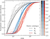 |
Fig. 12. Signal-to-noise ratio (S/N) distribution for IE, YE, and HE channels in the ultracool catalogue. The median S/N values are 10, 24, and 37, respectively. Dashed lines are distributions for the entire catalogue of ultracool candidates. Solid lines trace the variation of the S/N distribution with the IE − YE colour. In NISP, redder (cooler) objects tend to have higher S/N on average, while in the VIS band, the opposite is true and the difference between the red and blue is more pronounced. |
The majority of objects in the Q1 catalogue are extragalactic sources. Fortunately, these objects occupy a different part of the bluebottle diagram than substellar objects, as is shown in Fig. 13. Our cross-match with the Simbad database placed galaxies (e.g. Gaia Collaboration 2020, Straatman et al. 2016, Balestra et al. 2010, Cameron et al. 2011, and Le Fèvre et al. 2004), quasars (e.g. Tie et al. 2017, Gaia Collaboration 2020, and Xue et al. 2016), other active galactic nuclei (AGNs; e.g. Shim et al. 2013, Abbott et al. 2021, and Poulain et al. 2020), and supernovae (Gaia Collaboration 2020, Cappellaro et al. 2015, Cappellaro et al. 2005, and Lunnan et al. 2013) on the extragalactic branch that overlaps with the bluebottle ‘knee’ (late K and early M dwarfs), but extends above the stellar main sequence. On the other hand, Tu et al. (2025) report the photometric and spectroscopic similarity in the near-infrared between the L- and T-type brown dwarfs, high-redshift galaxies, and ‘little red dots’ (a recently discovered new type of object hypothesised to represent faint and/or highly reddened AGNs at high redshift; Matthee et al. 2024). They found good agreement between their candidate brown dwarf spectra and the models, and realised their extragalactic nature only when their inferred distances placed them more than a few kiloparsecs away. While our spectroscopic classification indicates a contamination rate of up to 67% beyond IE = 24 (Sect. 5), this value should be considered an upper limit due to the low quality of spectra at such faint magnitudes. A more reliable contamination estimate will only be possible after future repeated visits of the EDFs, when proper-motion measurements become available.
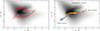 |
Fig. 13. Contamination with extragalactic sources is negligible in the UCD parameter space of the bluebottle diagram. Both plots show a distribution of the entire (unfiltered) Q1 catalogue. Left: Red contours mark the shape of the bluebottle diagram. Right: Objects in common between Euclid and Simbad: black dots are QSOs, AGNs, supernovae, or galaxies; and yellow dots are stars. Brown dwarfs (red dots) are from Zhang et al. (2024). |
The 10-Gyr PARSEC isochrone (Bressan et al. 2012; Pastorelli et al. 2020) shows that the asymptotic giant branch (AGB) reaches the cool tip of the bluebottle diagram (late L dwarfs; see Fig. 5). However, since the lifetime of the AGB stars is only a few million years (e.g. Ventura et al. 2018), these stars are very rare. It is thus unlikely that our sample of UCD candidates is contaminated with such evolved stars.
6.3. Metal-poor ultracool dwarfs
Our UCD selection is based on the IE − YE colour of the solar-metallicity objects. To investigate how this criterion affects the detection of metal-poor UCDs, we prepared a set of solar-metallicity and metal-poor models in the following way.
The public ATMO2020 isochrones are available only for solar metallicity. To explore the variation in the expected theoretical distribution in the YE − HE = f(IE − YE) diagram of ultracool objects with decreasing metallicity, we turned to the Sonora Bobcat grid of cloudless models (Marley et al. 2021).
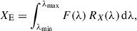
For [Fe/H]= − 0.5 and 0.0, for all values of temperature in the grid (200 to 2400 K) and for three values of the surface gravity (log g [cm s−2] = 3, 4, and 5), we computed Euclid equivalent magnitudes in each of the filters (X = IE, YE, or HE) by evaluation of the integral
 (1)
(1)
where RX(λ) is the transmission profile of a Euclid filter (provided by the Filter Profile Service, Rodrigo et al. 2024), F(λ) is the Sonora spectral flux expressed as a wavelength-dependent quantity, and λmin and λmax are the end wavelengths of the Sonora spectrum.
We compare the models in Fig. 14. They more or less overlap in the parameter space of M and L UCDs. We therefore cannot trace metal-poor objects in that part of the bluebottle diagram. On the other hand, the models predict considerably bluer YE − HE colours for T dwarfs. There is one candidate T dwarf (OBJECT_ID = −603476608509828998) that lies below the rest of the sample, but it has not yet been spectroscopically confirmed to be a UCD.
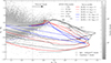 |
Fig. 14. Bluebottle diagram with the ATMO and Sonora models. The latter are provided for two sets of metallicities: solar (red curves); and [M/H] = −0.5. While we cannot isolate metal-poor M and L dwarfs, the models predict a notable colour spread with metallicity for T dwarfs in this diagram. |
6.4. Comparison with the Dark Energy Survey
Known UCDs in the literature are generally much brighter than our candidates. However, the cross-match with more than 19 000 photometric candidate UCDs from the Dark Energy Survey (DES; dal Ponte et al. 2023) yielded UCD candidates in common in EDF-S and EDF-F. In total, there are 188 DES candidates in the Q1 sky regions. We found Euclid counterparts for 125 of them; 56 do not meet our filtering criteria. The remaining 7 were not found within the 1 arcsec cross-matching radius, and might potentially have high proper motions. Most of the 125 objects in common have their spectra available in Euclid and belong to the C1 and C2 groups; many of them have their spectral types determined. A relation between IDES and IE was used to convert the DES magnitudes into the Euclid system and directly compare their distributions. Figure 15 shows that most of them have magnitudes between IE = 22 and 25, which is about the detection limit in DES. This distribution lies in the fainter half of the C1 and C2 groups and strengthens the case that these objects are true UCDs, as the candidates were selected photometrically using two independent methods and surveys.
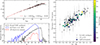 |
Fig. 15. Cross-match with the photometric UCD candidates from the Dark Energy Survey (dal Ponte et al. 2023). We found 125 objects in common. Left: Relation between IE and IDES. It is used to translate the DES data onto the Euclid scale and compare the magnitude distributions. Because DES covers about 100 times larger area of the sky than Q1 (EDF-N is not covered), the objects shared between the two surveys tend to fall within the magnitude range where most of the overall objects are found – between magnitudes 22 and 25. Right: A correlation between the YE − HE and JVHS VIKING − Ks, VHS VIKING colours (available in the dal Ponte et al. 2023 catalogue). A tight relation supports a reliable cross-match. More than 60% of them were spectroscopically classified into C1 and C2 groups (black circles), and 25% have a spectral type determined. |
6.5. Expected detections of UCDs in the forthcoming Euclid data releases
This work demonstrates the potential of Euclid to systematically detect numerous field UCDs. While they cover the EDF regions, the Q1 catalogues have essentially the same depth of data as the planned EWS. The results of this paper can therefore be directly used to estimate the number of expected ultracool detections over 14 000 deg2 of the sky that Euclid is going to visit, and which corresponds to about one third of the entire celestial sphere.
Our detection of 5306 candidate UCDs in 63 deg2 of Q1 data gives an average6 density of approximately 100 UCDs per deg2, and 20 L and T dwarfs per deg2. For comparison, the density in DES that detected 20 000 UCDs in 5000 deg2 is four objects per deg2 (and about three L and T dwarfs per deg2; dal Ponte et al. 2023). The density in the Galactic plane would be larger, but these regions will not be observed by Euclid. We can therefore expect to detect about 1.4 million UCDs in the final data release of the EWS. Of these, about 300 000 are expected to be L and T dwarfs. Similarly, we can anticipate the detection of more than 2600 T dwarfs with the method used in this paper. These are lower limits, since the present catalogue is not yet complete and does not fully utilise the potential of the data.
These overall numbers are consistent with theoretical predictions. For example, Solano et al. (2021) estimated that Euclid was going to photometrically detect around 1 million objects in the NISP bands in the EWS. However, they estimated that the JE band, which was not used in our study, is the most sensitive to UCDs. It should be able to observe and detect about 2 million L dwarfs, 1 million T dwarfs, and a select number of Y dwarfs in the thin disc, as well as many objects in the thick disc, and even some halo objects. Conversely, the estimates for the VIS detector were about 100 times lower.
This particular catalogue of UCDs from the Q1 data release is based only on one visit of the EDFs, while Euclid is going to repeatedly observe them during the lifetime of the mission, and thus increase the detection limit by approximately 2 mag in each band. Our catalogue will therefore be improved in future, both for new and deeper observations, and the UCD selection methods.
7. Conclusions
This work presents a first catalogue of 5306 photometric UCD candidates in the deep fields of Euclid’s Q1 data release. It includes approximately 1200 L and T dwarf candidates. Out of the full sample, 546 candidate UCDs were spectroscopically confirmed; 26 of them are T dwarfs and 329 are L dwarfs. The catalogue is limited to objects with high-quality photometry and prioritises low contamination over completeness. Future work will call for a complementary search that explores fainter sources in the NISP data.
We provide empirical IE − YE, IE − JE, IE − HE, YE − JE, YE − HE, and JE − HE colours for each UCD spectral type. A comparison with the metal-poor Sonora Bobcat models shows that we cannot easily isolate metal-poor L dwarfs in the bluebottle diagram (i.e. the IE − YE versus YE − HE colour-colour diagram). However, metal-poor T dwarfs are expected to have colours different from their solar-metallicity counterparts.
We assessed Euclid’s capability to identify UCD candidates based on its photometric passbands, in comparison with the spectroscopic detections reported by Dominguez-Tagle et al. (2025). We outline the strengths and limitations of the photometric approach for selecting UCD candidates. As the analysis is based on the Q1 data release – which reaches the same depth as the planned Euclid Wide Survey – our results provide a direct projection of the number and types of UCDs expected to be detected over the full 5-year mission.
Data availability
Full Tables A.1 and A.3 are available at the CDS via https://cdsarc.cds.unistra.fr/viz-bin/cat/J/A+A/711/A37.
Acknowledgments
We thank the anonymous referee for their comments, which helped to improve this work. Funding for MŽ, CDT, NS, ST, NV, JYZ, and ELM was provided by the European Union (ERC Advanced Grant, SUBSTELLAR, project number 101054354). ELM, NL, VB and JYZ acknowledge support from the Agencia Estatal de Investigación del Ministerio de Ciencia, Innovación y Universidades under grant PID2022-137241NB-C41. MRZO acknowledges funding support from the project PID2022-137241NB-C42 by the Spanish “Ministerio de Ciencia, Innovación y Universidades”. PC, DB, PMB, and ES acknowledge financial support from the Agencia Estatal de Investigación (AEI/10.13039/501100011033) of the Ministerio de Ciencia e Innovación through project PID2020-112949GB-I00 (Spanish Virtual Observatory https://svo.cab.inta-csic.es). PMB acknowledges financial support from the Instituto Nacional de Técnica Aeroespacial through grant PRE-OVE. DB has been funded by grant No. PID2019-107061GB-C61 and PID2023-150468NB-I00 by the Spain Ministry of Science, Innovation/State Agency of Research MCIN/AEI/ 10.13039/501100011033. NPB is funded by Vietnam National Foundation for Science and Technology Development (NAFOSTED) under grant number 103.99-2020.63. The authors wish to acknowledge the contribution of the IAC High-Performance Computing support team and hardware facilities to the results of this research. This work has made use of the Euclid Quick Release Q1 data from the Euclid mission of the European Space Agency (ESA), 2025, https://doi.org/10.57780/esa-2853f3b. The Euclid Consortium acknowledges the European Space Agency and a number of agencies and institutes that have supported the development of Euclid, in particular the Agenzia Spaziale Italiana, the Austrian Forschungsförderungsgesellschaft funded through BMK, the Belgian Science Policy, the Canadian Euclid Consortium, the Deutsches Zentrum für Luft- und Raumfahrt, the DTU Space and the Niels Bohr Institute in Denmark, the French Centre National d’Etudes Spatiales, the Fundação para a Ciência e a Tecnologia, the Hungarian Academy of Sciences, the Ministerio de Ciencia, Innovación y Universidades, the National Aeronautics and Space Administration, the National Astronomical Observatory of Japan, the Netherlandse Onderzoekschool Voor Astronomie, the Norwegian Space Agency, the Research Council of Finland, the Romanian Space Agency, the State Secretariat for Education, Research, and Innovation (SERI) at the Swiss Space Office (SSO), and the United Kingdom Space Agency. A complete and detailed list is available on the Euclid web site (www.euclid-ec.org). This publication makes use of VOSA, developed under the Spanish Virtual Observatory (https://svo.cab.inta-csic.es) project funded by MCIN/AEI/10.13039/501100011033/ through grant PID2020-112949GB-I00. VOSA has been partially updated by using funding from the European Union’s Horizon 2020 Research and Innovation Programme, under Grant Agreement no 776403 (EXOPLANETS-A). This research has made use of the Simbad and Vizier databases, and the Aladin sky atlas operated at the centre de Données Astronomiques de Strasbourg (CDS), and of NASA’s Astrophysics Data System Bibliographic Services (ADS). This research makes use of ESA Datalabs Navarro et al. (2024); datalabs.esa.int), an initiative by ESA’s Data Science and Archives Division in the Science and Operations Department, Directorate of Science. Software: astropy (Price-Whelan et al. 2018), NumPy (Harris et al. 2020), IPython (Pérez & Granger 2007), TOPCAT (Taylor 2005) and matplotlib (Hunter 2007).
References
- Abbott, T. M. C., Adamów, M., Aguena, M., et al. 2021, ApJS, 255, 20 [NASA ADS] [CrossRef] [Google Scholar]
- Balestra, I., Mainieri, V., Popesso, P., et al. 2010, A&A, 512, A12 [NASA ADS] [CrossRef] [EDP Sciences] [Google Scholar]
- Bertin, E., & Arnouts, S. 1996, A&AS, 117, 393 [NASA ADS] [CrossRef] [EDP Sciences] [Google Scholar]
- Best, W. M. J., Dupuy, T. J., Liu, M. C., et al. 2024, https://doi.org/10.5281/zenodo.13993077 [Google Scholar]
- Bishop, C. M. 2006, Pattern Recognition and Machine Learning (Springer) [Google Scholar]
- Bouy, H., Bertin, E., Moraux, E., et al. 2013, A&A, 554, A101 [NASA ADS] [CrossRef] [EDP Sciences] [Google Scholar]
- Bouy, H., Martín, E. L., Cuillandre, J.-C., et al. 2025, A&A, 696, A80 [NASA ADS] [CrossRef] [EDP Sciences] [Google Scholar]
- Bressan, A., Marigo, P., Girardi, L., et al. 2012, MNRAS, 427, 127 [NASA ADS] [CrossRef] [Google Scholar]
- Burgasser, A. J. 2014, Astron. Soc. India Conf. Ser., 11, 7 [Google Scholar]
- Burgasser, A. J., & Splat Development Team 2017, Astron. Soc. India Conf. Ser., 14, 7 [Google Scholar]
- Cameron, E., Carollo, C. M., Oesch, P. A., et al. 2011, ApJ, 743, 146 [Google Scholar]
- Cappellaro, E., Riello, M., Altavilla, G., et al. 2005, A&A, 430, 83 [NASA ADS] [CrossRef] [EDP Sciences] [Google Scholar]
- Cappellaro, E., Botticella, M. T., Pignata, G., et al. 2015, A&A, 584, A62 [NASA ADS] [CrossRef] [EDP Sciences] [Google Scholar]
- Carnero Rosell, A., Santiago, B., dal Ponte, M., et al. 2019, MNRAS, 489, 5301 [NASA ADS] [CrossRef] [Google Scholar]
- Chambers, K. C., Magnier, E. A., Metcalfe, N., et al. 2016, arXiv e-prints [arXiv:1612.05560] [Google Scholar]
- Cuillandre, J.-C., Bertin, E., Bolzonella, M., et al. 2025, A&A, 697, A6 [Google Scholar]
- Cutri, R. M., Skrutskie, M. F., van Dyk, S., et al. 2003, VizieR Online Data Catalog: II/246 [Google Scholar]
- Cutri, R. M., Wright, E. L., Conrow, T., et al. 2021, VizieR On-line Data Catalog: II/328 [Google Scholar]
- dal Ponte, M., Santiago, B., Carnero Rosell, A., et al. 2023, MNRAS, 522, 1951 [NASA ADS] [CrossRef] [Google Scholar]
- Desai, S., Armstrong, R., Mohr, J. J., et al. 2012, ApJ, 757, 83 [Google Scholar]
- Dominguez-Tagle, C., Žerjal, M., Sedighi, N., et al. 2025, ApJ, 991, 84 [Google Scholar]
- Epchtein, N., de Batz, B., Capoani, L., et al. 1997, The Messenger, 87, 27 [NASA ADS] [Google Scholar]
- Euclid Collaboration (Schirmer, M., et al.) 2022, A&A, 662, A92 [NASA ADS] [CrossRef] [EDP Sciences] [Google Scholar]
- Euclid Quick Release Q1, 2025, https://doi.org/10.57780/esa-2853f3b [Google Scholar]
- Euclid Collaboration (Cropper, M., et al.) 2025, A&A, 697, A2 [Google Scholar]
- Euclid Collaboration (Jahnke, K., et al.) 2025, A&A, 697, A3 [Google Scholar]
- Euclid Collaboration (Mellier, Y., et al.) 2025, A&A, 697, A1 [Google Scholar]
- Euclid Collaboration (Aussel, H., et al.) 2026, A&A, 711, A1 (Euclid Q1 SI) [Google Scholar]
- Euclid Collaboration (McCracken, H. J., et al.) 2026, A&A, 711, A2 (Euclid Q1 SI) [Google Scholar]
- Euclid Collaboration (Polenta, G., et al.) 2026, A&A, 711, A3 (Euclid Q1 SI) [Google Scholar]
- Euclid Collaboration (Romelli, E., et al.) 2026, A&A, 711, A4 (Euclid Q1 SI) [Google Scholar]
- Gaia Collaboration 2020, VizieR On-line Data Catalog: I/350 [Google Scholar]
- Garzón, F., Balcells, M., Gallego, J., et al. 2022, A&A, 667, A107 [CrossRef] [EDP Sciences] [Google Scholar]
- Harris, C. R., Millman, K. J., van der Walt, S. J., et al. 2020, Nature, 585, 357 [NASA ADS] [CrossRef] [Google Scholar]
- Hunter, J. D. 2007, Comput. Sci. Eng., 9, 90 [NASA ADS] [CrossRef] [Google Scholar]
- Kirkpatrick, J. D., Reid, I. N., Liebert, J., et al. 1999, ApJ, 519, 802 [NASA ADS] [CrossRef] [Google Scholar]
- Kirkpatrick, J. D., Reid, I. N., Liebert, J., et al. 2000, AJ, 120, 447 [NASA ADS] [CrossRef] [Google Scholar]
- Kirkpatrick, J. D., Marocco, F., Gelino, C. R., et al. 2024, ApJS, 271, 55 [NASA ADS] [CrossRef] [Google Scholar]
- Lawrence, A., Warren, S. J., Almaini, O., et al. 2007, MNRAS, 379, 1599 [Google Scholar]
- Le Fèvre, O., Vettolani, G., Paltani, S., et al. 2004, A&A, 428, 1043 [CrossRef] [EDP Sciences] [Google Scholar]
- Luhman, K. L. 2014, ApJ, 786, L18 [Google Scholar]
- Lunnan, R., Chornock, R., Berger, E., et al. 2013, ApJ, 771, 97 [NASA ADS] [CrossRef] [Google Scholar]
- Mace, G. N., Kirkpatrick, J. D., Cushing, M. C., et al. 2013, ApJS, 205, 6 [Google Scholar]
- Marley, M. S., Saumon, D., Visscher, C., et al. 2021, ApJ, 920, 85 [NASA ADS] [CrossRef] [Google Scholar]
- Martín, E. L., Delfosse, X., Basri, G., et al. 1999, AJ, 118, 2466 [Google Scholar]
- Martín, E. L., Phan-Bao, N., Bessell, M., et al. 2010, A&A, 517, A53 [Google Scholar]
- Martín, E. L., Žerjal, M., Bouy, H., et al. 2025, A&A, 697, A7 [NASA ADS] [CrossRef] [EDP Sciences] [Google Scholar]
- Matthee, J., Naidu, R. P., Brammer, G., et al. 2024, ApJ, 963, 129 [NASA ADS] [CrossRef] [Google Scholar]
- McMahon, R. G., Banerji, M., Gonzalez, E., et al. 2013, The Messenger, 154, 35 [NASA ADS] [Google Scholar]
- Miret-Roig, N., Bouy, H., Raymond, S. N., et al. 2022, Nat. Astron., 6, 89 [NASA ADS] [CrossRef] [Google Scholar]
- Mohandasan, A., Smart, R. L., Reylé, C., et al. 2025, A&A, submitted [arXiv:2503.22559] (Euclid Q1 SI) [Google Scholar]
- Mohr, J. J., Armstrong, R., Bertin, E., et al. 2012, in Software and Cyberinfrastructure for Astronomy II, eds. N. M. Radziwill, & G. Chiozzi, Int. Soc. Opt. Photonics (SPIE), 8451, 84510D [Google Scholar]
- Navarro, V., del Rio, S., Angel Diego, M., et al. 2024, in Space Data Management. Studies in Big Data, 141, 1 [Google Scholar]
- Palau, A., Huélamo, N., Barrado, D., Dunham, M. M., & Lee, C. W. 2024, New A Rev., 99, 101711 [Google Scholar]
- Pastorelli, G., Marigo, P., Girardi, L., et al. 2020, MNRAS, 498, 3283 [Google Scholar]
- Pérez, F., & Granger, B. E. 2007, Comput. Sci. Eng., 9, 21 [Google Scholar]
- Phillips, M. W., Tremblin, P., Baraffe, I., et al. 2020, A&A, 637, A38 [NASA ADS] [CrossRef] [EDP Sciences] [Google Scholar]
- Planck Collaboration XI. 2014, A&A, 571, A11 [NASA ADS] [CrossRef] [EDP Sciences] [Google Scholar]
- Poulain, M., Paolillo, M., De Cicco, D., et al. 2020, A&A, 634, A50 [NASA ADS] [CrossRef] [EDP Sciences] [Google Scholar]
- Price-Whelan, A. M., Sipőcz, B. M., Günther, H. M., et al. 2018, AJ, 156, 123 [NASA ADS] [CrossRef] [Google Scholar]
- Radigan, J. 2014, ApJ, 797, 120 [NASA ADS] [CrossRef] [Google Scholar]
- Radigan, J., Lafrenière, D., Jayawardhana, R., & Artigau, E. 2014, ApJ, 793, 75 [NASA ADS] [CrossRef] [Google Scholar]
- Reylé, C. 2018, A&A, 619, L8 [NASA ADS] [CrossRef] [EDP Sciences] [Google Scholar]
- Rodrigo, C., Cruz, P., Aguilar, J. F., et al. 2024, A&A, 689, A93 [NASA ADS] [CrossRef] [EDP Sciences] [Google Scholar]
- Shim, H., Im, M., Ko, J., et al. 2013, ApJS, 207, 37 [NASA ADS] [CrossRef] [Google Scholar]
- Skrutskie, M. F., Cutri, R. M., Stiening, R., et al. 2006, AJ, 131, 1163 [NASA ADS] [CrossRef] [Google Scholar]
- Solano, E., Gálvez-Ortiz, M. C., Martín, E. L., et al. 2021, MNRAS, 501, 281 [Google Scholar]
- Straatman, C. M. S., Spitler, L. R., Quadri, R. F., et al. 2016, ApJ, 830, 51 [NASA ADS] [CrossRef] [Google Scholar]
- Taylor, M. B. 2005, in Astronomical Data Analysis Software and Systems XIV, eds. P. Shopbell, M. Britton, & R. Ebert, ASP Conf. Ser., 347, 29 [Google Scholar]
- Tie, S. S., Martini, P., Mudd, D., et al. 2017, AJ, 153, 107 [Google Scholar]
- Tu, Z., Wang, S., Chen, X., & Liu, J. 2025, ApJ, 980, 230 [Google Scholar]
- Ventura, P., Karakas, A., Dell’Agli, F., García-Hernández, D. A., & Guzman-Ramirez, L. 2018, MNRAS, 475, 2282 [NASA ADS] [Google Scholar]
- Whitworth, A. 2018, arXiv e-prints [arXiv:1811.06833] [Google Scholar]
- Wright, E. L., Eisenhardt, P. R. M., Mainzer, A. K., et al. 2010, AJ, 140, 1868 [Google Scholar]
- Xue, Y. Q., Luo, B., Brandt, W. N., et al. 2016, ApJS, 224, 15 [Google Scholar]
- York, D. G., Adelman, J., Anderson, J. E., Jr, et al. 2000, AJ, 120, 1579 [Google Scholar]
- Zhang, J. Y., Lodieu, N., & Martín, E. L. 2024, A&A, 686, A171 [NASA ADS] [CrossRef] [EDP Sciences] [Google Scholar]
Available at e.g. the Spanish Virtual Observatory’s website.
The documentation is available online in the Euclid SGS Data Product Description Document.
Reddening in Euclid was estimated from the Planck dust map (Planck Collaboration XI 2014), which is two-dimensional, providing only upper limits for objects within our Galaxy (see Euclid Collaboration: Romelli et al. 2026, for more details).
The bluebottle is a stinging marine animal, similar to a jellyfish, from the genus Physalia.
The depth of the images varies across the field due to dithering (e.g. Euclid Collaboration: McCracken et al. 2026).
Appendix A: Tables
In Table A.1 we present the 60 UCDs from Zhang et al. (2024) that have been spectroscopically confirmed by Dominguez-Tagle et al. (2025) using Euclid NISP data. These are used as benchmark objects in this paper. In Table A.2 we list the seven confirmed T dwarfs and six candidates. In Table A.3 we list the main result of this paper, namely our catalogue of photometrically selected UCD candidates.
Benchmarks
Photometric T dwarf candidates
Photometric UCD candidates in the Q1 data release
All Tables
All Figures
|
Fig. 1. Morphological filters differentiate between extended sources and point sources. The filtering criteria (red lines for ELLIPTICITY and MUMAX_MINUS_MAG) are based on the benchmark UCDs (red dots; Zhang et al. 2024). Grey dots are sources from the entire Euclid catalogue. The right panel shows that while KRON_RADIUS is not used in the procedure, it correlates well with luminosity for the point sources. |
| In the text | |
|
Fig. 2. Magnitude distributions and signal-to-noise characteristics of the point-source catalogue. Left: Magnitude distributions for each point-source selection filter (we do not plot the FWHM filter). The most limiting is the S/N requirement that raises the completeness and detection limits to ensure a high quality of the point-source catalogue. Right: Signal-to-noise ratio as a function of luminosity. A cut at S/N = 4 is imposed. |
| In the text | |
|
Fig. 3. Magnitude distributions in the point-source catalogue. Completeness limits are approximately 23.5 for the NISP bands and 24.5 for VIS. The filtering procedure was not applied to the JE band, since it was not used in the candidate selection from the colour-colour diagram. |
| In the text | |
|
Fig. 4. Euclid colour-colour diagram. The offset between EDF-N and EDF-S is most prominent in the solar-like region at 0.1 < IE − YE < 0.4. |
| In the text | |
|
Fig. 5. Bluebottle diagram of point sources. The central sequence starts with white dwarfs below IE − YE < 0, continues with stars, and ends in the cool tip with UCDs at IE − YE ≳ 2.5. Their nature is confirmed with the benchmark UCDs from Zhang et al. (2024). We overplotted both the new photometric candidate T dwarfs from this work (symbols with error bars), and those that were spectroscopically confirmed (open circles), as listed in Table A.2. ATMO models (Phillips et al. 2020) indicate the UCD parameter space, while the PARSEC model traces main sequence and evolved stars with redder YE − HE. |
| In the text | |
|
Fig. 6. Zoom into the cool tip of the bluebottle diagram showing the benchmark objects (coloured dots with error bars). The spectral types are from Dominguez-Tagle et al. (2025). We overplotted typical positions for each spectral type from the curve fits (red squares) and ATMO models for a range of ages. |
| In the text | |
|
Fig. 7. Reverse cumulative distribution, showing how many objects are redder than the selected colour. There are 5306 objects redder than 2.5, which correspond to late M dwarfs, and 1200 objects redder than 2.9, which roughly correspond to L0 dwarfs. The red curve corresponds to objects whose spectra exhibit UCD features, whereas the blue line corresponds to objects with assigned spectral types. |
| In the text | |
|
Fig. 8. Bluebottle diagram focused on the UCDs. Models predict that early Y dwarfs are located in a horizontal band below the main bluebottle body. While there are many photometric candidates found there, none of them have been spectroscopically confirmed. We manually inspected the available spectra of the objects below the black line and found that most of them are not consistent with UCDs (black crosses). Apart from the T dwarfs, only seven other objects show UCD (or stellar) spectra. |
| In the text | |
|
Fig. 9. Magnitude distribution of the candidate UCDs with spectra (stacked histogram). Spectral types could be determined for 50% of the entire sample, limited by the S/N of the spectra. While spectral typing is limited at low S/N, spectroscopic confirmation is still possible nearly down to the VIS detection limit. |
| In the text | |
|
Fig. 10. Typical colours for each spectral type. Black dots represent individual objects, crosses mark objects rejected during the sigma-clipping fitting, and open circles indicate objects excluded from the fit due to suspected variability. The black line shows a polynomial fit to the relation. The grey area in the O − C plots represents the standard deviation of the residuals. |
| In the text | |
|
Fig. 11. Completeness for the colour bins in the bluebottle diagram. Despite its very high sensitivity, VIS is the most limiting instrument for the detection of UCDs in Euclid. The top panels show a group of bright objects at ≈(0, 0), which are quasars. |
| In the text | |
|
Fig. 12. Signal-to-noise ratio (S/N) distribution for IE, YE, and HE channels in the ultracool catalogue. The median S/N values are 10, 24, and 37, respectively. Dashed lines are distributions for the entire catalogue of ultracool candidates. Solid lines trace the variation of the S/N distribution with the IE − YE colour. In NISP, redder (cooler) objects tend to have higher S/N on average, while in the VIS band, the opposite is true and the difference between the red and blue is more pronounced. |
| In the text | |
|
Fig. 13. Contamination with extragalactic sources is negligible in the UCD parameter space of the bluebottle diagram. Both plots show a distribution of the entire (unfiltered) Q1 catalogue. Left: Red contours mark the shape of the bluebottle diagram. Right: Objects in common between Euclid and Simbad: black dots are QSOs, AGNs, supernovae, or galaxies; and yellow dots are stars. Brown dwarfs (red dots) are from Zhang et al. (2024). |
| In the text | |
|
Fig. 14. Bluebottle diagram with the ATMO and Sonora models. The latter are provided for two sets of metallicities: solar (red curves); and [M/H] = −0.5. While we cannot isolate metal-poor M and L dwarfs, the models predict a notable colour spread with metallicity for T dwarfs in this diagram. |
| In the text | |
|
Fig. 15. Cross-match with the photometric UCD candidates from the Dark Energy Survey (dal Ponte et al. 2023). We found 125 objects in common. Left: Relation between IE and IDES. It is used to translate the DES data onto the Euclid scale and compare the magnitude distributions. Because DES covers about 100 times larger area of the sky than Q1 (EDF-N is not covered), the objects shared between the two surveys tend to fall within the magnitude range where most of the overall objects are found – between magnitudes 22 and 25. Right: A correlation between the YE − HE and JVHS VIKING − Ks, VHS VIKING colours (available in the dal Ponte et al. 2023 catalogue). A tight relation supports a reliable cross-match. More than 60% of them were spectroscopically classified into C1 and C2 groups (black circles), and 25% have a spectral type determined. |
| In the text | |
Current usage metrics show cumulative count of Article Views (full-text article views including HTML views, PDF and ePub downloads, according to the available data) and Abstracts Views on Vision4Press platform.
Data correspond to usage on the plateform after 2015. The current usage metrics is available 48-96 hours after online publication and is updated daily on week days.
Initial download of the metrics may take a while.