| Issue |
A&A
Volume 700, August 2025
|
|
|---|---|---|
| Article Number | A9 | |
| Number of page(s) | 30 | |
| Section | Planets, planetary systems, and small bodies | |
| DOI | https://doi.org/10.1051/0004-6361/202452972 | |
| Published online | 29 July 2025 | |
Hydride ion continuum hides absorption signatures in the NIRPS near-infrared transmission spectrum of the ultra-hot gas giant WASP-189b★
1
Observatoire de Genève, Département d’Astronomie, Université de Genève,
Chemin Pegasi 51,
1290
Versoix,
Switzerland
2
Institut Trottier de recherche sur les exoplanètes, Département de Physique, Université de Montréal, Montréal,
Québec,
Canada
3
Centre Vie dans l’Univers, Faculté des sciences de l’Université de Genève,
Quai Ernest-Ansermet 30,
1205
Geneva,
Switzerland
4
Instituto de Astrofísica e Ciências do Espaço, Universidade do Porto, CAUP, Rua das Estrelas,
4150-762
Porto,
Portugal
5
Departamento de Física e Astronomia, Faculdade de Ciências, Universidade do Porto, Rua do Campo Alegre,
4169-007
Porto,
Portugal
6
Observatoire du Mont-Mégantic,
Québec,
Canada
7
Univ. Grenoble Alpes, CNRS, IPAG,
38000
Grenoble,
France
8
Department of Physics, University of Toronto,
Toronto,
ON
M5S 3H4,
Canada
9
Departamento de Física Teórica e Experimental, Universidade Federal do Rio Grande do Norte, Campus Universitário,
Natal,
RN
59072-970,
Brazil
10
Department of Physics & Astronomy, McMaster University,
1280 Main St W,
Hamilton,
ON
L8S 4L8,
Canada
11
Department of Physics, McGill University,
3600 rue University,
Montréal,
QC
H3A 2T8,
Canada
12
Department of Earth & Planetary Sciences, McGill University,
3450 rue University,
Montréal,
QC
H3A 0E8,
Canada
13
Instituto de Astrofísica de Canarias (IAC), Calle Vía Láctea s/n,
38205
La Laguna, Tenerife,
Spain
14
Departamento de Astrofísica, Universidad de La Laguna (ULL),
38206
La Laguna, Tenerife,
Spain
15
European Southern Observatory (ESO),
Karl-Schwarzschild-Str. 2,
85748
Garching bei München,
Germany
16
Space Research and Planetary Sciences, Physics Institute, University of Bern,
Gesellschaftsstrasse 6,
3012
Bern,
Switzerland
17
Consejo Superior de Investigaciones Científicas (CSIC),
28006
Madrid,
Spain
18
Bishop’s Univeristy, Dept of Physics and Astronomy,
Johnson-104E, 2600 College Street,
Sherbrooke,
QC
J1M 1Z7,
Canada
19
Department of Physics and Space Science, Royal Military College of Canada,
PO Box 17000, Station Forces,
Kingston,
ON,
Canada
20
European Southern Observatory (ESO),
Av. Alonso de Cordova 3107, Casilla
19001,
Santiago de Chile,
Chile
21
Planétarium de Montréal,
Espace pour la Vie, 4801 av. Pierre-de Coubertin, Montréal,
Québec,
Canada
22
Light Bridges S.L., Observatorio del Teide, Carretera del Observatorio, s/n Guimar,
38500
Tenerife, Canarias,
Spain
23
Institute of Space Sciences (ICE, CSIC), Carrer de Can Magrans S/N, Campus UAB,
Cerdanyola del Valles
08193,
Spain
24
Institut d’Estudis Espacials de Catalunya (IEEC),
08860
Castelldefels (Barcelona),
Spain
★★ Corresponding author: valentina.vaulato@unige.ch
Received:
12
November
2024
Accepted:
3
March
2025
Context. Ultra-hot Jupiters showcase one-of-a-kind extreme atmospheric conditions, including the dissociation of molecules into atomic species, ionisation, and significant day-to-night temperature contrasts. The proximity to their host stars exposes ultra-hot Jupiters to intense stellar irradiation, enabling high temperatures that drive noteworthy contributions to the overall opacity by hydride ions (H−), potentially obscuring features of metals in the near-infrared transmission spectrum.
Aims. This work aims to detect atomic, ionic, and molecular species in the atmosphere of WASP-189b (H, He, Fe, Ti, V, Mn, Na, Mg, Ca, Cr, Ni, Y, Ba, Sc, Fe+, Ti+, TiO, H2O, CO, and OH). A focus is placed on (i) understanding the role of H− as a source of absorption continuum opacity, and (ii) retrieving the relative hydride-to-Fe abundance using combined optical and near-infrared data.
Methods. We present two transits of WASP-189b gathered simultaneously in the optical with HARPS and in the near-infrared with NIRPS, supported by photometric light curves from EulerCam and ExTrA. Transmission spectra were analysed via cross-correlation to detect a planet’s absorption features and to increase the signal-to-noise ratio of potential detections. Additionally, atmospheric retrievals quantified relative abundances by fitting the overall metallicity, and abundance proxies for TiO, H−, and e−.
Results. Only atomic iron is detected in HARPS data (S/N~5.5). However, no Fe is detected at near-infrared wavelengths, likely due to the H− continuum dampening. Atmospheric retrievals on HARPS only and HARPS+NIRPS combined suggest that the hydride-to-Fe ratio exceeds equilibrium model predictions by ~0.5 dex, hinting at a strong ionisation rate for hydrogen atoms. Including NIRPS data helps to constrain the H− abundance, as well as set an upper limit on the free electron density, which is unconstrained from the HARPS-only retrieval. These results emphasise the impact of H− as a non-negligible source of continuum absorption opacity impeding the detection of planetary absorption features in the near-infrared transmission spectrum of WASP-189b.
Key words: instrumentation: spectrographs / methods: observational / techniques: spectroscopic / planets and satellites: atmospheres / planets and satellites: composition / planets and satellites: gaseous planets
© The Authors 2025
 Open Access article, published by EDP Sciences, under the terms of the Creative Commons Attribution License (https://creativecommons.org/licenses/by/4.0), which permits unrestricted use, distribution, and reproduction in any medium, provided the original work is properly cited.
This article is published in open access under the Subscribe to Open model. Subscribe to A&A to support open access publication.
1 Introduction
Ultra-hot Jupiters are a class of gas giant exoplanets with short orbital periods around hot, early-type (typically A or F) host stars (e.g. Hellier et al. 2009; Collier Cameron et al. 2010; West et al. 2016; Delrez et al. 2016; Gaudi et al. 2017; Lund et al. 2017; Talens et al. 2018; Anderson et al. 2018). These planets are exposed to intense stellar irradiation, leading to equilibrium temperatures above 2000 K and giving rise to extreme physico-chemical and climatic conditions. Ultra-hot Jupiters experience cloud-free daysides, the dissociation of molecules into atomic and ionic species (Kitzmann et al. 2018; Parmentier et al. 2018; Hoeijmakers et al. 2018, 2019), and strong day-to-night temperature contrasts and winds (Arcangeli et al. 2019; Seidel et al. 2019, 2021; Seidel et al. 2023) resulting in the dissociation or recombination and ionisation of molecular hydrogen (H2; Bell & Cowan 2018). Condensation of metals can happen at the terminator as material from the dayside is transported to the nightside by the day-to-night flow (Ehrenreich et al. 2020). On the other hand, evaporation of metals happens on the dayside, where the overall temperature of the atmosphere of the planet increases. Metallic species such as iron (Fe) or titanium (Ti) and vanadium (V) and their oxides are thought to play an important role in driving inversions in the temperature profile (Evans et al. 2017; Lothringer et al. 2018), boosting the atmospheric scale height H(z) = kBT(z)/μ(z)g(z) (where z is the altitude; kB is the Boltzmann constant; T(z), μ(z), and g(z) are the temperature, mean-molecular weight, and acceleration of gravity, respectively) at high altitudes. Indeed, the scale height is impacted by the local mean-molecular weight and temperature of the atmosphere (gravity can be assumed to be constant). As a result of the dependence of the scale height on the temperature and mean-molecular weight, the dayside is “puffier” than the nightside. The effect is twofold. Firstly, the dayside is much hotter than the nightside. Secondly, atomic hydrogen on the dayside is subject to thermal dissociation, resulting in a factor 2 decrease in mean-molecular weight. This dichotomy gives ultra-hot gas giants a peculiar terminator shape as seen during transit, characterised by two halves of a different thickness (Pluriel et al. 2020; Wardenier et al. 2021, 2023), making them particularly well-suited for transit spectroscopy. Transmission spectroscopy benefits from the stellar light being filtered by the atmosphere of the planet. Indeed, during the transit event, the stellar photons are absorbed and scattered depending on the wavelength, the chemical composition, and the structure of the planetary atmosphere (Seager & Sasselov 2000). The transmission spectrum of a planetary atmosphere can exhibit the following: (i) absorption features caused by electronic transitions in atoms and ions or vibrational, rotational, and rovibrational transitions in molecules, and (ii) scattering continuum due to atoms and molecules (Rayleigh regime) or aerosols (Mie regime). Ultrahot gas giants are predicted to bear atomic and ionic species on their dayside atmospheres, with a composition close to chemical equilibrium (Kitzmann et al. 2018) and patchy nightside clouds due to the difficulty to form aerosols at such high temperatures (Komacek et al. 2022).
Under clear atmospheres (i.e. in the absence of Mie scattering and significant continuum absorption caused by clouds, hazes, and aerosols), one would expect the contrast of absorption features to be maximised in the transmission spectrum of exoplanetary atmospheres. However, Arcangeli et al. (2018) argue that in the atmospheres of ultra-hot gas giants, the contrast of potential spectroscopic features must be dampened by the absorption continuum caused by the negative hydrogen ion (hereafter, hydride or H−). This anion has long been known to constitute ‘a major factor ruling the structure of late-type stellar atmospheres’ (Wildt 1939, ‘late-type’ meaning here cooler than F-type ones), which share effective temperatures akin to those of ultra-hot gas giant daysides. In atmospheric layers where the electron density is high (due to the photoionisation of alkali metals), the hydrogen atom can hold a second electron in a bound state due to the highly polarised structure of the neutral H atom (Gray 2021). This extra electron can be set free by any photon impacting with an energy larger than 0.7542 eV, or a wavelength shorter than 1.644 μm. This photoelectric ionisation of the hydride ion thus results in a so-called bound-free absorption continuum covering all spectral domains bluer than the H band (from 1.1 to 1.4 μm). In the optical, bound-free transitions are dominant, but their contribution decreases beyond 1.4 μm, where free-free interactions to form hydride become more significant in the infrared domain.
Furthermore, the H− opacity overlaps with important absorbing species such as titanium and vanadium oxide (Parmentier et al. 2018). Similarly, the near-infrared domain typically dominated by strong molecular bands in cooler planets becomes muted in ultra-hot Jupiters due to the combination of molecular dissociation and the increased presence of the hydride continuum. Constraining the abundance of hydride relative to other species in the near-infrared could thus help disentangling the different sources of opacity at shorter wavelengths, or vice versa.
In this work, we report on new transit observations of the ultra-hot Jupiter WASP-189b (Anderson et al. 2018) obtained in the framework of the Guaranteed Time Observations (GTO) of the NIRPS consortium. The Near-InfraRed Planet Searcher (NIRPS1, Bouchy et al. 2017; Wildi et al. 2022; Bouchy et al. 2025) is a new ultra-stable, near-infrared (Y J H, from 0.95 to 1.8 μm), high-resolution fibre-fed spectrograph installed at the ESO 3.6 m telescope in La Silla, Chile. NIRPS is designed to observe simultaneously with HARPS (Mayor et al. 2003), which covers the optical range from 378 up to 691 nm. Thanks to HARPS and NIRPS observations, we can obtain high-resolution spectra (R = λ/Δλ ranging from ~80 000 in the near-infrared to 120 000 in the optical) from the edge of the near-ultraviolet to the H band, with a ~250 nm gap between ~700 and 950 nm. The NIRPS GTO consortium exploited these capabilities to design a large survey of exoplanetary atmospheres (Allart et al. 2025), composed of several sub-programmes: (i) a transit survey, (ii) a dayside emission survey, as well as programmes dedicated to study (iii) young exoplanets, (iv) multi-planetary systems, (v) planetary system architectures and (vi) a TRAPPIST-1 dedicated initiative. The transit survey aims at observing 75 giant planets over 5 years for a wide range of irradiation levels and masses to derive population-level trends in the context of planet formation and evolution.
WASP-189b is the most irradiated target of the NIRPS GTO transit survey and one of the first transiting planets observed with NIRPS. WASP-189b (Anderson et al. 2018) is one of the most highly irradiated Jovian planets known to date: it is a massive (Mp ≈ 2 MJ) gas giant orbiting the hot (Teff = 8000 K) A-type star on a circular and strongly misaligned, almost polar orbit (3D obliquity Ψ = 85.4 ± 4.3°; Lendl et al. 2020). A summary of the WASP-189 planetary system is provided in Table 1. Observations of occultations of the planet by its star with the CHEOPS space telescope (Benz et al. 2021) yielded an estimation of the dayside brightness temperature of 3 435 ± 27 K (Lendl et al. 2020) and a precise planet radius of 1.619 ± 0.021 RJ. Analysing two archival optical transits obtained with HARPS, Stangret et al. (2022) reported on the detections of absorption features by neutral and singly ionised iron (FeI and FeII, respectively) and neutral titanium (TiI). These chemical species were identified from the cross-correlation function (CCF) of the transmission spectrum with template models, as well as tentative, single-line detections of the hydrogen Balmer lines (Hα, Hβ), and the calcium CaII H and K lines. Furthermore, Prinoth et al. (2022, 2023, 2024) performed a broad optical survey of atomic and molecular species in the atmosphere of WASP-189b by jointly analysing transit observations obtained with the ESPRESSO (Pepe et al. 2021), MAROON-X (Seifahrt et al. 2020, 2018), HARPS, and HARPS-N (Cosentino et al. 2012) spectrographs. Prinoth et al. (2023) reported significant detections of a variety of species (H, Na, Mg, Ca, Ca+, Ti, Ti+, TiO, V, Cr, Mn, Fe, Fe+, Ni, Sr, Sr+, and Ba+). Gandhi et al. (2023) retrieved abundances of a subset of these metals using four archival HARPS-South and HARPS-North transits combined, finding most to be in agreement with chemistry predictions of a solar-composition atmospheric model; only Fe is found to be depleted (Fe constraint to be below the stellar Fe/H value by ~0.7 dex) likely because a large amount of iron is thought to be ionised. Additionally, Yan et al. (2020) detected atomic Fe emission lines in dayside spectra of WASP-189b with HARPS-N. At longer wavelengths, Yan et al. (2022) detected carbon monoxide (CO) in the thermal emission spectra observed with the GIANO-B near-infrared spectrograph (Claudi et al. 2017). At shorter wavelengths, Sreejith et al. (2023) observed the magnesium MgII h and k lines with the CUTE (France et al. 2023) ultraviolet space telescope. Recently, Lesjak et al. (2025) reported on blueshifted cross-correlation signals of CO and Fe likely due to day-tonight winds from CRIRES+ K-band dayside observations of WASP-189b. Together, these studies provide a comprehensive view of the atmospheric dynamics and chemical complexity of WASP-189b, highlighting the interplay between neutral and ionised species and the mechanisms that maintain the thermal structure of this ultra-hot Jupiter.
In this work, we report on the first near-infrared high-resolution spectroscopic NIRPS observations of the transit of WASP-189b. Section 2 describes the spectroscopic and photometric observations. Section 3 describes the stellar properties, the telluric and preparatory corrections, and details on the cross-correlation transmission spectroscopy method used. In Section 5, we present the results of both the cross-correlation and the atmospheric retrieval analyses, and discuss their implications.
Planetary and stellar relevant parameters.
2 Observations
2.1 Spectroscopic transit observations with NIRPS and HARPS
We observed two transits (Figure 1) of WASP-189b across the disc of its bright host star HD 133112 (V = 6.6, J = 6.2) on 2023-04-24 (Night 1) and on 2023-04-06 (Night 2), as part of the ESO GTO program 111.2506 (PI: F. Bouchy). The transit duration (from contact point 1 and contact point 4) is ~4 hours (see Table 1), and the total observing time (transit duration + baseline before ingress and after egress) was ~6 hours for both nights. We observed the target simultaneously with HARPS in High Accuracy Mode (HAM) and NIRPS in High Efficiency (HE) mode. The adaptive optics system provides NIRPS with a main High Accuracy (HA) fibre covering a diameter of 0.4 arcsec on the sky for a greater spectral resolution (maximum of 96 300 for the science fibre), and a larger HE fibre with a field of view of 0.9 arcsec (see Bouchy et al. 2025, for more details). The NIRPS HE mode allows to reduce the impact of modal noise at the reddest wavelengths while keeping a good spectral resolution (maximum of 80 300 for the science fibre) with respect to the HA mode. Both instruments have two fibres A and B, located on the target and the sky, respectively. Between 1.3765 and 1.3973 μm two echelle spectral orders (104 and 105) are missing due to OH doped absorption in the optical fibre train. These two orders also correspond to the unusable domain of the deep telluric water band between J and H photometric bands. The transit time series acquired on 2023-04-24 exhibits an approximately one hour gap which occurred during the transit window (from 05:38 UT until 06:35 UT) due to a communication issue between NIRPS and the telescope. This explains why we gathered a different total number of spectra between NIRPS and HARPS during the first night (difference of 20 spectra). The observation log can be found in Table 2 and in Figure 1.
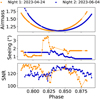 |
Fig. 1 Observing conditions during Night 1 and Night 2 as a function of phase (phase = (BJD − Tc)/P, where BJD is the barycentric Julian date, Tc = 2458926.5 days is the mid-transit time, and P = 2.724033 days is the period, which are all from Lendl et al. 2020). The top panel and mid panel illustrate the airmass and the average atmospheric Dimm seeing evolving during the nights, respectively. The Dimm seeing is averaged for each observations (i.e. average between the start and the end of each observation). The bottom panel shows the S/N (extracted from the fits header) changing during the nights. |
2.2 Simultaneous photometry with EulerCam and ExTrA
Photometric observations contemporaneous to spectroscopic ones may refine the ephemeris of the system, improving orbital parameters such as the planet’s orbital period, the transit duration, mid-transit time, and to assess the stellar variability (e.g. absence of flares and spots) if any. This allows for more accurate predictions of future transit events.
In parallel to our NIRPS-HARPS observation on 2023-04-06, we observed the transit with EulerCam (Lendl et al. 2012) and ExTrA (Bonfils et al. 2015). The lightcurves are reported in Figure 2. EulerCam is a 4k × 4k CCD camera installed at the 1.2 m Swiss Euler telescope in La Silla, Chile. The observations were taken in Johnson-V filter and the exposure time was set to 30 seconds. The ExTrA facility consists of three 0.6-m telescopes feeding a near-infrared, multi-object spectrograph in La Silla, Chile. The observations were taken on the three telescopes mode and the exposure time was set to 60 seconds. We lost ingress of the transit observation as the dome was vignetting in the eastern horizon up to 42 degrees. Additionally, we had to discard light curves from telescopes one and two, due to high photometric scatter.
To obtain the system parameters, we fit the observed light curves with transit models computed using CONAN (Lendl et al. 2017). The free parameters include the mid-transit time, duration, transit depth, impact parameter, and quadratic limb-darkening coefficients. We choose wide Gaussian priors centred on the values from Lendl et al. (2020). The quadratic limb-darkening coefficients were centred around estimates from the LDCU2 package (Deline et al. 2022). LDCU is a modified version of the Python routine implemented by Espinoza & Jordán (2015) that computes the limb-darkening coefficients and their corresponding uncertainties using a set of stellar intensity profiles accounting for the uncertainties on the stellar parameters. The stellar intensity profiles are generated based on two libraries of synthetic stellar spectra: ATLAS (Kurucz 1979) and PHOENIX (Husser et al. 2013). In addition, we fix the period and eccentricity to literature values of 2.724033 days and 0, respectively. To account for the correlated noise in our observations, we fit a photometric baseline model along with the pure transit model. The baseline model is determined by iteratively fitting different models involving air mass, exposure time, sky background, shifts (both coordinate and abscissa), and the Full-With at Half-Maximum (FWHM) of the stellar Point Spread Function (PSF), minimising the Bayesian Information Criterion (BIC). The optimal baseline for EulerCam observations comprises of a second-order polynomial on the x-shifts of stellar PSF and a first order polynomial on time and air mass. In addition, we simultaneously fit the light curves with a Gaussian Process (GP), using a Matérn 3/2 kernel, to account for the correlated noise at short timescales. The full set of priors and posteriors from our analysis are listed in Table A.1. From our analysis, we do not refine the system parameters reported by Lendl et al. (2020). Even though simultaneous photometry does not always improve the system parameters, it still strengthens the reliability of the overall analysis by offering additional context and cross-validation. In addition, the derived system parameters are consistent with Lendl et al. (2020).
Log of NIRPS and HARPS transit observations.
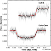 |
Fig. 2 De-trended light curve obtained with ExTrA and EulerCam, respectively. The transit model is over-plotted in red. The root-mean-squares of EulerCam and ExTrA light curves are 1206 and 1620 ppm, respectively. |
3 Stellar properties
The most irradiated giant exoplanets are found around early-type stars, typically A- and F-type stars (e.g. KELT-9b, TOI-2109b, WASP-189b, and WASP-33b, Gaudi et al. 2017; Wong et al. 2021; Anderson et al. 2018; Collier Cameron et al. 2010). These stars are hotter than the Sun and their photospheres exhibit fewer spectroscopic features broadened by their fast rotation speed. Indeed, WASP-189b orbits a catalogued fast rotating A-type star, HD 133112 (HR 5599) (see Table 1 for the main system parameters). Generally, A-type stars are not favourable targets for the detection of exoplanets in radial velocities because they exhibit few, rotationally broadened spectral lines (requiring specific approaches or tools, e.g. Galland et al. 2005). Despite the expected small signal induced by a close-in, planetary origin companion orbiting a line-poor and fast rotating star, Collier Cameron et al. (2010) confirmed for the first time a gas giant planet transiting the rapidly rotating, A-type, main-sequence star HD 15082 (also known as WASP-33). HD 133112 was first classified as an A5m star by Cowley (1968) and listed with a ‘doubtful’ A4m classification in the catalogue of chemically peculiar stars (Renson & Manfroid 2009). In the discovery paper for WASP-189b (Anderson et al. 2018), the Am classification was ruled out based on the strength of the CaII K line in their HARPS spectra. Lendl et al. (2020) re-analysed the stellar properties using archival HARPS spectra as well as synthetic models. They derived stellar abundances typical of Am stars and measured a stellar rotational velocity of v sin i⋆ = 93.1 ± 1.7 km s−1. They concluded from this that the stellar inclination should be close to 90°. These authors also found clear evidence for gravity darkening of the stellar photosphere. Saffe et al. (2021, 2022) performed a new analysis of the chemical abundances of the star and challenged its Am classification. Both Prinoth et al. (2022) and Prinoth et al. (2023) classify WASP-189 as A-type star, without further investigation about the peculiar subclass.
4 Methods
All spectra are reduced by the automated HARPS and NIRPS Data Reduction Softwares (DRS version 3.5 and 3.2.0, respectively; Pepe et al. 2021), which yield the one- and two-dimensional stellar spectra (S1D and S2D) corrected for the Barycentric Earth Radial Velocity (BERV). We describe below the additional data correction and analysis steps that are still needed to obtain the transit transmission spectra of the planetary atmosphere. The starting point of this analysis are the HARPS S1D_A and NIRPS S1D_TELL_CORR_A3 FITS files (Subsection 4.1), which are the one-dimensional spectra produced by the stitching of the deblazed 71 and 72 echelle spectral orders of NIRPS and HARPS, respectively. After the flux extraction, the spectra have Norder × 4096. Indeed, the detector is provided with 4096 × 4096 pixels containing all the spectral orders. For each night of observations, we thus work on a temporal series of spectra f(λ, t) = f(λ, t)|BERV (i.e. provided in the barycentric frame of reference).
4.1 Correction for telluric features
To mitigate the influence of Earth’s atmosphere on HARPS stellar spectra, we use molecfit (Smette et al. 2015; Kausch et al. 2015), as the 3.5 version of the data reduction pipeline does not include corrections for telluric features. molecfit corrects for telluric lines (H2O, O2) impacting the optical band covered by HARPS. For this purpose, we follow the methodology outlined in Allart et al. (2017). The molecfit workflow takes our one-dimensional spectra f(λ, t) as input and fits them using a synthetic transmission spectrum generated by a line-by-line radiative transfer code, which includes the list of telluric absorption lines within the relevant wavelength ranges.
Infrared spectra are significantly contaminated by hydroxyl (OH) telluric emission lines originating in Earth’s mesosphere from 0.61 μm to 2.62 μm (Rousselot et al. 2000), as well as telluric absorption lines (H2O, O2, CH4, CO2) heavily polluting J and H photometric bands. Moreover, deep water bands make spectral orders 104 and 105 unusable (between 1376.5 and 1397.3 nm). The NIRPS data reduction pipeline adapted from the ESPRESSO pipeline (Pepe et al. 2021) takes care of correcting the telluric OH airglow in the sky-fibre channel, and the telluric absorption lines to produce S1D_TELL_CORR_A and S2D_TELL_CORR_A FITS files4. For near-infrared NIRPS spectra, we use the automated correction of telluric features developed by Allart et al. (2022) and implemented in the data reduction pipeline (version 3.2.0). We choose this over using molecfit as a telluric correction approach as we found that, while both perform similarly (see Appendix E for further details), the DRS correction can correct for both absorbing and emitting telluric features up to three times the continuum noise according to cross-correlation computations performed on stellar data using a built telluric mask. Indeed, the derived root-mean-square of the correlation peak is in agreement with what was obtained and shown for ESPRESSO in the visible wavelength range by Allart et al. (2022). To address the presence of telluric residuals, especially prevalent in the infrared domain around 1.4 μm and 1.8 μm where H2O deep telluric bands dominate, we perform an iterative sigma-clipping process over the telluric profile used to fit the scientific stellar spectra. The threshold optimisation has also been done by visual inspection of the post-correction spectra and cross-correlation maps (obtained as described in Section 5.1.2). We adopt a threshold of 50% to filter out persistent telluric absorption lines in the optical range of wavelengths. HARPS optical spectra are little impacted by deep telluric lines and, consequently, less affected by telluric residuals needy to be removed. For near-infrared wavelengths, where telluric lines can saturate (especially those belonging to water bands), and residuals are more likely to remain after the telluric correction, we increase the threshold to 90%, resulting in 36.7% of the NIRPS data being masked. After correcting for the Earth’s atmosphere, we identify and mask any spurious spikes remaining in the data.
4.2 Normalisation of the spectra and outlier correction
We normalise the telluric-corrected spectra by dividing them by the median flux of each spectrum, ![$\[\tilde{f}(\lambda, t)=f(\lambda, t) / f(\langle\lambda\rangle, t)\]$](/articles/aa/full_html/2025/08/aa52972-24/aa52972-24-eq5.png) . We also correct for cosmic rays which may randomly hit the detector and produce signals unrelated to the star or planet, and any other effect resulting in an outlier value that escaped the automated reduction pipeline. To do this, we calculate a median spectrum
. We also correct for cosmic rays which may randomly hit the detector and produce signals unrelated to the star or planet, and any other effect resulting in an outlier value that escaped the automated reduction pipeline. To do this, we calculate a median spectrum ![$\[\tilde{f}(\lambda,\langle t\rangle)\]$](/articles/aa/full_html/2025/08/aa52972-24/aa52972-24-eq6.png) for each night and we subtract it from the normalised, telluric-corrected spectra. We apply a 5σ-clipping filter along the spectral dimension to identify outlying pixels and discard them from our spectra (Allart et al. 2017).
for each night and we subtract it from the normalised, telluric-corrected spectra. We apply a 5σ-clipping filter along the spectral dimension to identify outlying pixels and discard them from our spectra (Allart et al. 2017).
4.3 Transmission spectroscopy
Once the spectra have been cleaned and normalised, we Doppler-shift all the in-transit and out-of-transit spectra into the stellar rest frame,
![$\[\left.\tilde{f}(\lambda, t)\right|_{\star}=\tilde{f}\left[\lambda\left(1+\frac{v_{\mathrm{sys}}+\Delta r v_{\star}(t)}{c}\right), t\right],\]$](/articles/aa/full_html/2025/08/aa52972-24/aa52972-24-eq7.png) (1)
(1)
where vsys is the systemic velocity (vsys = −24.5 km s−1, Anderson et al. 2018), and Δrv⋆(t) is the radial velocity variation of the star caused by the reflex motion of WASP-189b measured from the Sun barycentre rest frame, to create the ‘master-in’ ℱin(λ) and ‘master-out’ spectra ℱout(λ), respectively,
![$\[\left.\mathcal{F}_{\text {out }}(\lambda)\right|_{\star}=\left.\frac{1}{n_{\text {out }}} \sum_{t \in \text {out}} \tilde{f}(\lambda, t)\right|_{\star},\]$](/articles/aa/full_html/2025/08/aa52972-24/aa52972-24-eq8.png) (2)
(2)
where nout is the number of spectra taken out-of-transit for nights 1 and 2 (see Table 2).
To obtain the spectral ratio ℜ(λ) (Brown 2001), we divide the corrected, normalised in-transit spectra ![$\[\tilde{f}(\lambda, t \in \mathrm{in})\]$](/articles/aa/full_html/2025/08/aa52972-24/aa52972-24-eq9.png) by the master-out spectrum. Since the planet radial velocity is substantially changing during the transit, we then realign the calculated spectral ratios into the planetary rest frame before co-adding them (e.g. Wyttenbach et al. 2015; Allart et al. 2017; Seidel et al. 2019; Mounzer et al. 2022),
by the master-out spectrum. Since the planet radial velocity is substantially changing during the transit, we then realign the calculated spectral ratios into the planetary rest frame before co-adding them (e.g. Wyttenbach et al. 2015; Allart et al. 2017; Seidel et al. 2019; Mounzer et al. 2022),
![$\[\Re(\lambda)=\sum_{t \in \text {in}}\left[\left.\frac{\left.\tilde{f}(\lambda, t)\right|_{\star}}{\left.\mathcal{F}_{\text {out }}(\lambda)\right|_{\star}}\right|_p\right]=\sum_{t \in \text {in}}\left[\left.\mathrm{r}(\lambda, t)\right|_p\right],\]$](/articles/aa/full_html/2025/08/aa52972-24/aa52972-24-eq10.png) (3)
(3)
![$\[\left.\mathfrak{r}(\lambda, t)\right|_p=\left.\mathfrak{r}\left[\lambda\left(1+\frac{r v_p(t)}{c}\right), t\right]\right|_{\star},\]$](/articles/aa/full_html/2025/08/aa52972-24/aa52972-24-eq11.png)
where 𝔯(λ, t), the ‘temporal spectral ratio’, represents our time series of transit transmission spectra (e.g. Ehrenreich et al. 2020), and rvp is the radial velocity of the planet in the stellar rest frame (see Equation (6)).
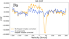 |
Fig. 3 One-dimensional cross-correlation function based on HARPS data calculated for neutral iron before (orange) and after (blue) correcting for the stellar contamination in the form of the two-component Rossiter-McLaughlin effect. |
4.3.1 Removal of the Doppler shadow
While transiting the star, the planet partially obscures the rotating stellar surface, producing the well-known Rossiter–McLaughlin effect (Rossiter 1924; McLaughlin 1924), usually presented as a redshift followed by a blueshift in the stellar radial velocities integrated over the full stellar disc (for an aligned, prograde system). The Rossiter-McLaughlin effect distorts all spectral lines in the integrated stellar spectrum and typically creates residuals in transit cross-correlation time series when it is not accounted for. Specifically, the distortions appear in the cross-correlation functions during the transit phases as a combination of a dark trace in emission (the ‘Doppler shadow’) and a second negative broad component in the velocity versus time space (cf. Figures 3 and 4). The Doppler shadow can create absorption-like features that can be mistaken from atmospheric features (Casasayas-Barris et al. 2022). The slope and width of the Doppler shadow depend on the projected spin-orbit angle (λ), and the projected stellar rotation velocity (v sin i⋆), respectively. In simple cases (low λ, low v sin i⋆), the Doppler shadow can be reasonably well fitted with a Gaussian, then subtracted to reveal the absorption signature of the transiting planetary atmosphere (e.g. Ehrenreich et al. 2020). WASP-189b, however, is transiting its rapidly rotating host star (v sin i⋆ = 93.1 km s−1) on a strongly misaligned, almost polar orbit (true obliquity Ψ = 85.4°5), leaving a noticeable residual structure on the maps (see Figure 4) obtained from cross-correlating our transit spectra with a template model (see Sections 5.1.2 and 5.1.3). To correct for the Rossiter-McLaughlin effect (both components) in the cross-correlation (Section 5.1.2) and velocity-velocity maps (Section 5.1.3), we use the Gaussian fitting approach. Step (i) is to fit the Doppler shadow with a Gaussian function for each time series as varying the phase (Ehrenreich et al. 2020; Prinoth et al. 2022), and after to subtract the best-fit model from the cross-correlation. The residuals are the cross-correlation values which cannot be modelled and explained by the first Gaussian function, most likely linked to the second component of the Rossiter-McLaughlin effect. Therefore, step (ii) consists in fitting and subtracting a second Gaussian model to the residual data. We set initial guesses for the parameters of the Gaussian profiles, namely for the amplitude (A), the peak velocity (μ), the width of the Gaussian (σ), and a constant value for the continuum baseline (c). The initial guesses for both Gaussian components are reported in Table B.1. Correcting for the two-component Rossiter-McLaughlin effect smooths the continuum level and increases the signal-to-noise ratio of the cross-correlation signal. Figure 3 illustrates the 1D cross-correlation function (cross-correlation function versus velocity) based on HARPS data calculated for neutral iron before and after correcting for the stellar contamination in form of the two-component Rossiter-McLaughlin effect.
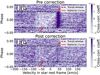 |
Fig. 4 Cross-correlation map based on HARPS data with no correction of the Rossiter-McLaughlin effect. The top panel shows the pre-correction scenario. The thick emitting dark vertical strip around 50 km s−1 is the first component of the Rossiter-McLaughlin contamination, that is called Doppler shadow. The wide absorbing feature from ~−80 km s−1 up to ~25 km s−1 is the second component of the stellar contamination. Bottom panel: the post-correction scenario once the best Gaussian fits are subtracted from the cross-correlation. |
5 Results and discussion
5.1 Signatures in the transit transmission spectrum of WASP-189b
5.1.1 Hydrogen and helium lines
We perform a visual inspection of the transit transmission spectrum ℜ(λ) to search for signatures of the excited atomic hydrogen in the HARPS and NIRPS range, and metastable helium in the NIRPS range. Several Balmer lines of HI fall within the HARPS range (Hα to Hζ), with Hα (λ = 656.3 nm), Hβ (λ = 486.1 nm), Hγ (λ = 434.0 nm), and Hδ (λ = 410.2 nm) having been previously detected in the atmosphere of the ultra-hot gas giant KELT-9b (Yan & Henning 2018; Wyttenbach et al. 2020). Hα (and possibly Hβ) absorption signal has been detected in several other ultra-hot or bloated gas giants (e.g. Borsa et al. 2021; Seidel et al. 2023). The NIRPS range covers lines from the Paschen series (Paβ λ = 1282 nm to Paϵ λ = 954.6 nm) as well as the Brackett break (Br∞ λ = 1458 nm). To date, one detection of the Paβ line was reported in the literature (Sánchez-López et al. 2022), also for KELT-9b. We do not detect absorption signatures in any of the above-mentioned hydrogen lines (see Appendix C). While Prinoth et al. (2022, 2023, 2024) report on a detection of hydrogen lines from their CCF analysis of WASP-189b (Hα at 656.46 nm), these authors made use of eight observation epochs using not only HARPS and HARPS-N but also MAROON-X and ESPRESSO at 8-meter-class telescopes. As a result, they obtained a much higher signal-to-noise ratio in the optical than this study, which is based on two observation epochs with HARPS. Given that here we only utilise two HARPS transits, it is not surprising that we do not have the sensitivity to recover the same detections as Prinoth et al. (2022, 2023, 2024).
The triplet lines of metastable helium around 1.083 μm represent another potential probe of the upper atmosphere of a gaseous planet (Spake et al. 2018; Allart et al. 2018). Indeed, helium atoms can accumulate in the upper atmosphere and experience strong irradiation from the star. The intense stellar radiation causes atmospheric heating and expansion. The heating can push the helium atoms into an excited state, specifically into a metastable state. Thus, the helium atoms in metastable state can strongly absorb near-infrared radiation at 1.083 μm in form of a triplet (Spake et al. 2018). The signature of escaping helium atoms has been detected in several exoplanets and near-infrared high-resolution spectroscopy is especially well suited to achieve this (e.g. Allart et al. 2018; Nortmann et al. 2018; Salz et al. 2018). However, the transit signature of helium arises from the absorption of light by excited helium atoms (Oklopčić & Hirata 2018). Allart et al. (2023) also argued that a specific irradiation environment is needed to allow for a large population of excited atoms to build. These environments include the vicinity of K dwarfs, while A-type dwarfs are thought not to be suited due to a lack of chromospherically driven extreme ultraviolet flux. It is thus not a surprise that none of the triplet lines are visible in the transit transmission spectrum of WASP-189b (see Figure 5). A non-detection of the helium triplet is either a lack of helium in the atmosphere (unlikely for such a Jupiter planet), or it is not populated. In the latter, either the planet does not receive the correct amount of energy to excite the escaping helium atoms, or the helium atoms are shielded or deep enough in the atmosphere of the planet to not escape. Meanwhile, Allart et al. (2025) report on a clear detection of helium around the warm Saturn WASP-69b-in orbit around a K star– from three observation epochs, showing that NIRPS is indeed sensitive to this signature and thus, given the similar sensitivity of these data sets, our non-detection can be indeed attributed to the lack of a sufficient population of metastable helium in the exosphere of WASP-189b to produce significant excess absorption.
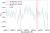 |
Fig. 5 Transmission spectrum of WASP-189b around the metastable helium triplet (vertical dashed red lines). Grey dots with error bars represent the entire transmission spectrum at native resolution, and cyan dots with uncertainties are the binned spectrum. No trace of metastable helium triplet is found in WASP-189b from atomic line inspection of its transmission spectrum, as expected given the theory of Oklopčić & Hirata (2018). |
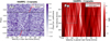 |
Fig. 6 Neutral Fe cross-correlation from two transits of WASP-189b observed with the HARPS spectrograph. Left panel: cross-correlation time series corrected for the Rossiter–McLauglin contribution. The planetary trail follows the Keplerian motion in red, and it is bound within the transit window (first and fourth contact transit phases indicated by horizontal black dashed line). Right panel: Kp−vsys diagram. The black dashed lines denote the expected vsys and Kp from Prinoth et al. (2023). The region enclosed in the cyan dotted box is used for the calculation of the S/N used throughout the entire map. Features around +50 and −50 km/s are residuals of the Rossiter-McLaughlin correction fitting and not due statistical fluctuations (Section 4.3.1). |
5.1.2 Cross-correlation functions of other atoms and molecules
With the inspection of HI Balmer, HeI and NaI lines (the latter being not detected from the transmission spectrum of WASP-189b), most chemical species have spectral features too weak to allow to detect the effect of absorption features on individual lines. Instead, it is possible to search for transit signals in their cross-correlation functions 𝒞 (Snellen et al. 2010). This approach has proven extremely successful on ultra-hot gas giants, allowing to unveil a large amount of atoms and ions in several such objects (Hoeijmakers et al. 2018, 2019; Borsa et al. 2021; Kesseli et al. 2022). Prinoth et al. (2022, 2023) recently adopted this approach to probe the atmosphere of WASP-189b in the optical. These authors reported a vast amount of atomic, ionic, and molecular signatures, for example TiO being present in the gaseous state in ultra-hot planets (thanks to their high temperatures), and known to be a relevant source of opacity due to its strong absorption bands in both the optical and near-infrared.
While most previous works studying the atmosphere of WASP-189b have been in the optical, the HARPS+NIRPS combination presented here covers a broader spectral domain than previous studies (including Prinoth et al. 2022, 2023), albeit with a lower sensitivity, since it is only based on two transits. Thus, we focus our attention on retrieving the species with the most ubiquitous spectral signatures, namely neutral iron, while still attempting to detect other species: Ti, V, Mn, Na, Mg, Ca, Cr, Ni, Y, Ba, Sc, Fe+, Ti+, TiO, H2O, CO, and OH.
We cross-correlate our transit spectra 𝔯(λ, t) with a template model of a transmission spectrum (T (v)) computed assuming a solar composition in chemical equilibrium at a uniform temperature T = 3000 K (adapted from Anderson et al. 2018). The atmospheric model used is further described in Section 5.2. We calculate 𝒞 at time t, for velocity shifts, v, between ± 200 km s−1 in steps of 0.5 km s−1,
![$\[\mathcal{C}(v, t)=\sum_{i=0}^N \mathfrak{r}_i(\lambda, t) T_i(v),\]$](/articles/aa/full_html/2025/08/aa52972-24/aa52972-24-eq12.png) (5)
(5)
where 𝔯i(λ, t) is the time series of N transmission spectra as function of time t and wavelength λ, namely each pixel in the transmission spectrum at a given time t, and Ti(v) are the computed model spectra Doppler shifted to a velocity v. The cross-correlation thus computed generates two-dimensional cross-correlation maps for each chemical element tested.
Following the cross-correlation method, we recover a neutral iron signal in the HARPS optical data of WASP-189b combining the two-transit observations (Figures 4, 6, and 7). The excess absorption falls at a velocity (between −50 and +50 km s−1 in the cross-correlation trail map) consistent with numerous previous works (Stangret et al. 2022; Prinoth et al. 2022, 2023) and matches the expected amplitude based on injection-recovery tests (Section 5.2.2). In contrast, we do not detect a neutral iron signature in the near-infrared NIRPS data6 (also when combining the two transits; see Figure 8).
5.1.3 Velocity-velocity maps
The two-dimensional cross-correlation time series are transformed into velocity-velocity diagrams (so called Kp–vsys maps, Brogi et al. 2012) by phase-folding the planetary signal for different orbital configurations. The maximum S/N is obtained when the cross-correlation functions are co-added along the trail corresponding to the motion of the planet in the velocity space. Each trail is given by the Keplerian equation:
![$\[r v\left(t, K_p\right)=K_p ~\sin~ (2 \pi \phi(t))+v_{\mathrm{sys}},\]$](/articles/aa/full_html/2025/08/aa52972-24/aa52972-24-eq13.png) (6)
(6)
where Kp is the semi-amplitude of the radial velocity of the planet; ϕ(t) is the planetary orbital phase, and vsys = Δvsys is the systemic velocity (here set at zero km s−1 because spectra were already shifted to the stellar rest frame before cross-correlating). The systemic velocity is shifted as varying the Kp values within the range from 50 km s−1 to 300 km s−1 in steps of 0.5 km s−1. We choose a wide range for the orbital radial velocity of the planet around the expected velocity (Kp = 200.7 km s−1, Prinoth et al. 2023) following the method described in Brogi et al. (2012). Cross-correlation time series and Kp–vsys maps computed with Fe template for HARPS and NIRPS are shown in Figures 6, 8, and 7, respectively. To calculate the S/N, (i) we select a “noise boxy region” in the velocity space far away from where the planetary signal is expected, and free of artificial features and residuals from both telluric and Rossiter-McLaughlin corrections (between Kp ∈ [−75, −25] km s−1 and vsys ∈ [150, 300] km s−1 for both HARPS and NIRPS, i.e. the cyan dashed box in Figure 6) to estimate the 1-σ noise level; (ii) we calculate the standard deviation of this noise box region, and eventually (iii) we compute the ratio between in-transit cross-correlation values summed up and the noise estimated according to point i) and ii). When computing cross-correlations from NIRPS spectra, the cross-correlation maps exhibit a non-negligible continuum, unrelated to any planetary signal. This is likely a consequence of the method used to compute the cross-correlation function (Equation (5)), which is statistically more akin to a cross-variance rather than Pearson’s correlation coefficients (Rodgers & Nicewander 1988). In Pearson’s correlation, the data and template are mean-subtracted, effectively removing any baseline offset. Thus, we fit a spline function for each time step (namely, to each row of the cross-correlation map) to model the continuum level and subtract it. Instead of fitting a single global polynomial (which might poorly capture local variations or overfit the data), splines fit low-degree polynomials in each region between the knots. We set the knots at −100, −50, 0, 50, and 100 km s−1, and choose a third order polynomial to fit the regions. Once the spline is fitted to each row (for each time slice), the resulting fitted values represent the “continuum” or broad underlying shape of the cross-correlation. This continuum is eventually subtracted from the original cross-correlation values for each velocity and time step. This effectively removes the broad trends, leaving behind the smaller, more significant cross-correlation features (such as dips from spectral lines).
The iron signature we significantly detect in the optical with HARPS (S/N ~ 5.5 at Kp,detection = 223.5 km s−1) appears blueshifted in the Kp–vsys map (Figure 6). Since we expect the planetary signal to be at zero-velocity in the planet’s rest frame, we measure the offset of the signature by fitting a Gaussian function to the peak in the S/N versus velocity (Figure 7). We find the neutral iron feature to be blueshifted by −5.54 ± 0.44 km s−1. We compute the uncertainty associated with the velocity shift as the square root of the variance. In their survey of ultra-hot gas giants, Gandhi et al. (2023) noted a net and ubiquitous blueshift of the order of 1–7 km s−1 in ultra-hot Jupiter atmospheres, including WASP-189b. Furthermore, Prinoth et al. (2022, 2023) mentioned non-significantly but blueshifted signatures indicative of day-to-night winds and flows (Seidel et al. 2020, 2021; Seidel et al. 2023) in the atmosphere of WASP-189b. Hence, our finding is consistent with previous literature results. Moreover, we build the ΔKp−vsys diagram in the case of the neutral iron detection with HARPS (Figure 7). According to Wardenier et al. (2023), the ΔKp is calculated as ΔKp = Kp − Kp,measured, being Kp = 200.7 ± 4.9 km s−1 the expected semi-amplitude of the radial velocity of the planet (Prinoth et al. 2023), and Kp,measured = K⋆ (M⋆/Mp) ≃ 194.7 ± 2.27 m s−1 the measured velocity. Values for K⋆, M⋆, and Mp can be found in Table 1. Thus, we calculate a ΔKp ≃ 6 km s−1. In this context, ΔKp−vsys maps help to compare with model predictions because the sign of ΔKp depends on the three dimensional distribution of a species across the atmosphere (Wardenier et al. 2023). Indeed, Wardenier et al. (2023) argue that ΔKp results positive in case of signals dominated by the trailing limb in the first half of the transit and by the leading limb in the second half. ΔKp > 0 might result surprising given the discussion in Wardenier et al. (2023), especially if we consider the opposite conclusion driven by the more significant atomic iron detection in Prinoth et al. (2022, 2023). However, it is worth mentioning that the value of ΔKp we estimate is within the error bar, considering the uncertainty of ±13 m s−1 on K⋆ by Anderson et al. (2018).
Apart from neutral Fe in the optical, we do not detect any of the chemical species aforementioned neither in HARPS, nor in NIRPS transmission spectrum of WASP-189b. However, we stress that these non-detections are not due to these species being absent in the near-infrared from the atmosphere of WASP-189b, neither are due to a lack of sensitivity (Section 5.2.2). The cross-correlation trail maps and Kp–vsys showing NIRPS and HARPS non-detections are reported in Appendix G and H together with upper limits (Tables G.1, H.1). We estimate the upper limits assuming a detection threshold of 3×1-σ, where 1-σ is the continuum noise level from the boxy region used to calculate the S/N, namely the cross-correlation value from that specific region in the velocity space. It is worth specifying that the line-contrast upper limits as calculated in this work can only be obtained with the choice of cross correlation in this manuscript, as its strength directly maps to the average line strength.
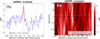 |
Fig. 7 Left panel: maximum S/N versus velocities at the measured Kp (blue curve). In red, the best-fit Gaussian to the Fe cross-correlation peak, whose centroid results blueshifted by −5.54 ± 0.44 km/s with respect to zero km/s. The positive peaks around ~40 km s−1, ~−60 km s−1, and the negative peak at ~−20 km s−1 are artefacts of the Rossiter-McLaughlin correction and not statistical fluctuations. Right panel: ΔKp−vsys diagram. The ΔKp is calculated as ΔKp = Kp − Kp,measured (Wardenier et al. 2023). The black dashed lines denote the expected vsys and Kp from Prinoth et al. (2023) (i.e. Kp = 200.7 km s−1). Features around +50 and −50 km/s are residuals of the Rossiter-McLaughlin correction fitting and not due statistical fluctuations (Section 4.3.1). |
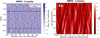 |
Fig. 8 Cross-correlation trail map (left panel) and Kp–vsys map (right panel) of NIRPS data, obtained with the reduction pipeline described in Section 4. Black dashed lines (right panel) denote the expected Kp determined from Prinoth et al. (2023), and vsys=0 km s−1. The colourmaps show a non-detection of Fe from two transits of WASP-189b observed with the NIRPS spectrograph. The observation gap occurred during the first transit on the night of 2023-04-24 is visible as a banded structure of higher scatter between phases 0.0 and 0.02 (left panel). |
5.2 Atmospheric forward modelling
We use SCARLET (Benneke & Seager 2012, 2013; Benneke 2015; Benneke et al. 2019; Pelletier et al. 2021) to generate transmission spectra of WASP-189b. SCARLET models use molecular cross sections for H2O (Polyansky et al. 2018), OH (Rothman et al. 2010), CO (Rothman et al. 2010; Li et al. 2015), and TiO (McKemmish et al. 2019) while atomic cross sections are from the VALD database (Ryabchikova et al. 2015) and continuum cross sections for H− (bound-free and free-free) are from Gray (2021). Molecular and atomic cross sections are computed using HELIOS-K (Grimm & Heng 2015; Grimm et al. 2021) and chemical equilibrium abundances are calculated using FastChem (Stock et al. 2018, 2022). We assume the thermal structure to be isothermal and the atmosphere to be cloud-free, which is a reasonable assumption considering the high temperature of ultra-hot gas giant atmospheres (Sing et al. 2016; Helling et al. 2021). We expect the iron signal to only probe the dayside of WASP-189b (Wardenier et al. 2023). We compute all models at a spectral resolution of 250 000 and convolve the spectra generated by the instrumental function to match NIRPS HE mode spectral resolution of R ~ 80 000 and HARPS HAM mode spectral resolution of R ~ 120 000.
For the cross-correlation, we generate a WASP-189b transmission template assuming a 1 × solar metallicity atmosphere at a temperature of 3000 K (based on Anderson et al. 2018), including opacity contributions from Fe, Ti, V, Mn, Mg, Ca, Cr, Ni, Y, Ba, Sc, C, Na, Fe+, Ti+, TiO, H2O, CO, OH, and H−. Contributions for all atomic, ionic, and molecular species of interest to the transmission spectrum are reported in Figures D.1 and D.2 in the Appendix D.
5.2.1 The role of hydride
While ultra-hot Jupiters such as WASP-189b are likely too hot to form clouds on their dayside or terminator regions, hydrogen anions act as an important source of continuum opacity (Section 1). The impact of the hydride on the transmission spectra must therefore not be neglected. The equations to estimate the bound-free and the free-free transitions are implemented in SCARLET following Gray (2021). Given the absorption coefficients8:
![$\[\alpha_{B F}(\lambda)=\left[a_0+a_1 \lambda+a_2 \lambda^2+a_3 \lambda^3+a_4 \lambda^4+a_5 \lambda^5+a_6 \lambda^6\right],\]$](/articles/aa/full_html/2025/08/aa52972-24/aa52972-24-eq14.png) (7)
(7)
![$\[\alpha_{F F}(\lambda)=\left[10^{f_0 \lambda+f_1 \lambda \log _{10} \theta+f_2 \log _{10}^2 \theta}\right],\]$](/articles/aa/full_html/2025/08/aa52972-24/aa52972-24-eq15.png) (8)
(8)
Gray (2021) calculates the H− bound-free and free-free crosssections as:
![$\[\sigma_{B F}(\lambda)=\frac{10^{-17}}{10^4} \alpha_{B F}\left(H^{-}\right),\]$](/articles/aa/full_html/2025/08/aa52972-24/aa52972-24-eq16.png) (9)
(9)
![$\[\sigma_{F F}(\lambda)=\frac{10^{-26}}{10^3} \alpha_{F F}\left(H^{-}\right).\]$](/articles/aa/full_html/2025/08/aa52972-24/aa52972-24-eq17.png)
Figure 9 shows how an example transmission spectrum generated by SCARLET is shaped by varying the abundance of hydride relative to Fe. The template spectrum includes Fe, TiO, OH, and contributions given by the hydride as a source of continuum absorption. Figure 9 is made with the purpose of visualising how the continuum absorption by the H− dampens the contrast of the neutral iron spectral lines along the whole range of wavelengths with respect to the continuum level. Specifically, the strength of iron lines depends on the relative abundance of hydride in the atmosphere of the planet at a given temperature and scale height. As the hydride abundance increases (holding the Fe abundance fixed), the contrast of Fe spectral lines decreases. Critically, the opacity contribution from H− can change the relative strength of spectral features in the optical and near-infrared (around 1.6 μm), in contrast to other continuum opacity sources (e.g. a grey cloud deck). The simultaneous wavelength coverage of the bound-free and free-free absorption continua provides an opportunity to better characterise the role of these two hydride contributions in ultra-hot atmospheres. While the cross-correlation method may be only weakly sensitive to continuum effects on the template, since it relies more on line positions, atmospheric retrievals are well-suited to constrain abundance ratios based on the relative contribution of different spectral features (e.g. Brogi & Line 2019).
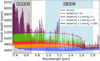 |
Fig. 9 Iron atmospheric model spectrum as a function of wavelength including contributions given by the hydride as a source of continuum absorption. In blue the atmospheric model for Fe, with no absorber added. In orange, the template spectrum including H− free-free as source of continuum opacity, boosted by a factor of 10. In red, the spectrum including a solar amount of H− bound-free. In the green and purple spectra, the bound-free contribution is boosted by a factor of 10 and 1000, respectively. The purple spectrum includes contributions by H2O beyond 1.6 μm. The grey and cyan coloured regions indicate HARPS and NIRPS coverage, respectively. It is worth mentioning that HARPS and NIRPS cover a similar fractional bandpass. We intentionally boost the continuum level differentiating the two main contributions to illustrate how the Fe spectrum changes accordingly. |
5.2.2 Injection-recovery results
We use the synthetic iron atmospheric spectrum of WASP-189b as forward-model to characterise the underlying planetary signal. In order to quantify the expected amplitude of the atmospheric absorption, we inject the iron atmospheric model into the NIRPS spectra after they have been corrected for tellurics, but before ℜ(λ) is calculated (see Section 4.3). For cleaner results, we inject the model into non-BERV corrected spectra. The injected data are then processed following the same reduction pipeline, described in Section 4, as the non-injected spectra, using the known system parameters listed in Table 1. Following Section 5.1.2, we compute the cross-correlation between the injected data and the modelled spectrum. We showcase two scenarios: (1) we cross-correlate the NIRPS transmission spectrum with the template model described in Section 5.2, considering only contributions given by atomic Fe spectral lines, and (2) we cross-correlate the data with the full template model, thus taking into account the hydride as source of continuum opacity. The results of the injection-recovery test in Figure 10 demonstrate that we are able to recover the injected neutral irononly signal at a signal-to-noise ratio of ~8, indicating that the NIRPS data are sufficiently sensitive to detect a pure iron template. However, when contributions by H− are also included, the injection-recovery test results in a non-detection of neutral iron. Therefore, we argue that the signal strength from a pure Fe template does not match the observations. Other opacity sources, likely hydride, could play a role in dampening the neutral iron signal such that it is not observed in near-infrared data. A similar injection-recovery test, but where the template is injected in emission instead of absorption (to cancel out the real neutral Fe absorption signal from WASP-189b’s atmosphere) in the HARPS data, finds that the Fe + H− template matches well the amplitude of the observed signal (see complementary Figure F.1 in Appendix F).
5.3 Atmospheric retrievals
In order to move beyond the cross-correlation method and infer posterior probabilities on atmospheric parameters of interest, we must use an adequate high-resolution likelihood prescription (e.g. Brogi & Line 2019; Gibson et al. 2020, 2022). Currently, the presented method to clean the data and remove contributions from the host star and Earth’s atmosphere to reveal the planetary signal relies on using a telluric model as well as a Doppler shadow correction (Sections 4.1 and 4.3.1). However, while the telluric correction is done at the spectral level, the average effect of the Doppler shadow is instead removed from the cross-correlation function. It is therefore not so obvious how to compute a likelihood, which is typically done at the spectral level, when including such a Doppler shadow correction. Nevertheless, this step cannot be neglected as removing contributions from the star is necessary given that the stellar photosphere also contains Fe, which could otherwise bias any inference of planetary atmospheric properties.
As accurately correcting for the Doppler shadow distortion on every stellar line residual at the spectral level would require a perfectly accurate model of the host star photosphere and is beyond the scope of the paper, we opt instead to proceed forward and retrieve the atmospheric properties of WASP-189b using the methodology presented by Pelletier et al. (2021, 2023). For this we now re-analyse the data, but instead starting from the telluric uncorrected order-by-order data products for both HARPS and NIRPS and using a Principal Component Analysis (PCA)-based approach to detrend the data of telluric and stellar contributions. Indeed while the cross-correlation maps calculated from the NIRPS DRS-corrected data still show some H2O residuals, even in the case where tellurics are masked aggressively (Figure G.1), we find that this data driven method is better at removing tellurics, albeit at the cost of potentially distorting the atmospheric trace of WASP-189b (we refer the reader to Appendix E for a detailed discussion). However, while PCA can alter and even remove an underlying planetary signal (Brogi & Line 2019; Cheverall & Madhusudhan 2024), this effect is less severe for short orbital period planets where atmospheric absorption lines are rapidly accelerating, such as in the case of WASP-189b observed in transmission. Nevertheless, reproducing the effect of the detrending procedure on the spectral line shapes and contrasts of the underlying planetary signal is critical in order to accurately infer properties of its atmosphere. As such, all likelihood calculations in the retrieval are made using such a ‘processed’ model that mimics the effect of PCA on spectral features (Pelletier et al. 2021, 2023). We opt to remove 10 principal components, although we tested removing anywhere between 3 and over 20 components, finding overall consistent results. We further discard from the analysis all exposures where the planetary trace overlaps with the Doppler shadow to avoid contamination from any potential remaining stellar residuals. Using this PCA-based approach, we similarly find an Fe absorption signature in the HARPS data (see Appendix Figure I.1) but do not detect an equivalent signature in the NIRPS data. This is not necessarily surprising given that Fe has much stronger spectral features in the optical than in the near-IR (Figure 9). Nevertheless, the presence of numerous Fe lines of various strengths spread across the HARPS and NIRPS wavelength ranges allows us to probe the effect of various continuum opacity sources. For example, the pseudo-continuum from TiO will affect the line contrast of Fe spectral features in and out of TiO absorption bands. Meanwhile, H− (bound-free) will instead dampen all Fe lines below ~1.5 μm roughly uniformly, while H− (free-free) will preferentially weaken lines at longer wavelengths.
We use the high-resolution atmospheric retrieval framework detailed in Pelletier et al. (2021, 2023); Pelletier et al. (2024); Bazinet et al. (2024) which uses SCARLET to produce transmission spectra, the CCF-to-log likelihood prescription of Gibson et al. (2020), and emcee (Foreman-Mackey et al. 2013) as a sampler. We run a retrieval first on the HARPS data alone, and then a retrieval also including the NIRPS data, for both transits simultaneously. Other than abundance parameters, the retrieval fits for the atmospheric temperature, the velocity parameters Kp and vsys, as well as a free broadening parameter. The temperature is assumed to be uniform across the atmosphere (isothermal). Kp and vsys are fitted rather than fixed as the observed position of the atmospheric signature of WASP-189b can differ from the values predicted for a uniform and static atmosphere. We also include an extra Gaussian broadening parameter as the observed signal is more extended (blurred) in Kp–vsys space than expected from the instrumental resolution only.
As thermal dissociation and ionisation are important in ultra-hot Jupiter atmospheres, especially at sub-millibar pressures probed by transmission spectroscopy, abundances of species can vary by orders of magnitude in pressure. As such, we opt against so called ‘free retrievals’ that parametrise the abundance of elements as uniform-in-pressure and instead compute abundance profile using FastChem, which takes into account ionisation and dissociation. However, in order to give the model some flexibility in exploring non-equilibrium scenarios, we fit for both an overall metallicity ([M/H]) controlling the abundances refractory elements as well as a separate metallicity for Ti-bearing species ([Ti/H]). Here [M/H] refers to the log10 metallicity relative to solar and controls the abundance of all non-Ti bearing species included in the retrieval (Fe, Fe+, Cr, Mg, V, Mn, Ca, Ni, Na, H2O, CO, and OH), with a value of [M/H] = 0.5 corresponding to an atmospheric composition for WASP-189b being 100.5× that of the Sun (Asplund et al. 2009). Meanwhile, [Ti/H] controls the abundances of TiO, Ti, and Ti+. The motivations for fitting [Ti/H] separately is because titanium species are often observed to be underabundant in ultra-hot Jupiter atmospheres, likely due to nightside cold-trapping (Hoeijmakers et al. 2020, 2024; Merritt et al. 2020; Maguire et al. 2023; Gandhi et al. 2023), in which case the TiO abundance can be greatly over-predicted by models (e.g. Pelletier et al. 2023; Pelletier et al. 2024). Similarly, the opacity contributions of H− (bound-free and free-free) will strongly depend on the availability of electrons in the atmosphere of WASP-189b, which is dependent on the ionisation of metals (Gray 2021). Given the plausibility that non-equilibrium processes play a role in affecting the abundances of H− and e−, we also fit for log10 multiplicative factors (log αH− and log αe−) to both the hydride and e− abundance profiles predicted by FastChem. A value of log αH− = 1 would therefore correspond to the H− abundance being 10× higher at all pressures than expected from equilibrium chemistry for the given composition (set by [M/H] and [Ti/H]) and temperature structure.
Our retrievals therefore have a total of eight parameters (Table 3), with the overall results shown in Figure 11. We find the overall metallicity [M/H] (mostly driven by Fe) to be well consistent with solar. Intriguingly, our retrieval provides a bounded constraint on the titanium metallicity [Ti/H] despite the lack of a cross-correlation detection of any Ti-bearing species. Rather, this constraint is driven by the retrieval preferring to add TiO bands as a source of pseudo-continuum. Interestingly, the retrieved [Ti/H] abundance comes out to be nearly the same as the overall metallicity. While normally one should be sceptical of retrieved posteriors on species not detected in cross-correlation, in this particular case TiO is known from higher S/N data to be present in the transmission spectrum of WASP-189b (Prinoth et al. 2022, 2023). Nevertheless, we do not consider this a robust detection of TiO and rather simply take it as further evidence that models of WASP-189b including TiO in its atmosphere are preferred.
The retrieval also constrains the abundance of H−, finding this source of opacity to be more prevalent than predicted from chemistry predictions. This may indicate that the continuum set by H− is more pronounced than expected. We note, however, that an over abundance of H− could also be the result of other sources of opacity in the atmosphere of WASP-189b unaccounted for in our models (e.g. metal oxides like VO, FeO, MgO, CaO, etc. or metal hydrides like FeH, MgH, SiH, AlH, CaH, etc.). The abundance of free electrons is unsurprisingly not well constrained when including HARPS only, with a much stricter upper limit obtained when including NIRPS. Overall, even though the cross-correlation detection of Fe is mostly driven by the HARPS data, the inclusion of NIRPS with a high sensitivity across near-infrared wavelengths is highly constraining, especially for H− and e−. The temperature is found to be around 3800 K, which is similar to what was found by Gandhi et al. (2023). Moreover, we retrieve a rotational broadening value of ≃36 km s−1, about one order of magnitude higher than the equatorial rotational velocity of the planet estimated to be of ≃3 km s−19. Indeed, transmission data are more sensitive to atmospheric dynamics, hence we could expect a rotational broadening parameter ≉ planet rotation rate. We surmise that the blurred atomic iron signal detected in HARPS optical data, and, consequently, the high retrieved rotational broadening parameter, are linked to the combination of the planet’s rotation rate, day-to-night winds (known in ultra-hot gas giants, Seidel et al. 2021), and super rotating jets, all acting to contribute various blue and red Doppler shifts which all together blur the signal. What found is consistent with Prinoth et al. (2022), who also explain the broadening of the spectral lines to be due to super-rotational winds and flows causing an exacerbation of the red- and blueshifts of the limbs.
Broadly speaking, all of our retrieved parameters are fairly consistent with the atmosphere of WASP-189b having a solarlike composition, with the exception that the H− bound-free contribution (in the form of the hydrogen anion abundance) appears to be elevated relative to what equilibrium chemistry predicts by about 0.5 dex (Figure 12). Interestingly, the H− continuum being slightly higher than expected has little implications for the detectability of metals with very deep absorption lines in the optical, as evident by the wealth of species that have already been detected in transmission on WASP-189b (e.g. Prinoth et al. 2023). However, this could mean that other elements or molecules that only have weaker spectral features (even if there are many), such as H2O, may be harder to detect in ultra-hot Jupiter atmospheres using transmission spectroscopy.
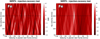 |
Fig. 10 Kp–vsys map showcasing the injection-recovery test on NIRPS data. Left panel: the injected iron atmospheric model includes contributions from the H− as a source of continuum opacity; the map shows no detection of atomic Fe in the near-infrared data of WASP-189b, consistent with non-injected results. Right panel: the injected iron atmospheric model does not include contributions from the hydride; in this case, the map shows a clear detection of neutral Fe in the near-infrared data. Black dashed lines denote the expected vsys and Kp determined from Prinoth et al. (2023). |
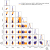 |
Fig. 11 Retrieved constraints on the atmospheric and orbital properties obtained from the observed two transits of WASP-189b. The orange shows the retrieval considering only the HARPS data, while the blue shows with the inclusion of NIRPS. Here the overall metallicity, as well as the titanium-only metallicity are well constrained to be near-solar. Meanwhile the H− abundance is slightly above expectations from solar model in chemical equilibrium. The inclusion of the NIRPS data is particularly helpful in constraining the H− abundance, as well as setting a strict upper limit on the free electron density, which is unconstrained from the HARPS-only retrieval. |
WASP-189b SCARLET atmospheric posteriors from the retrieval analysis on the HARPS and NIRPS time series combined.
6 Conclusions
This study presents an in-depth analysis of WASP-189b’s atmospheric composition using high-resolution transmission spectra from two transit time series gathered simultaneously with HARPS and NIRPS. A key finding is the detection of atomic Fe in the optical at a maximum S/N of ~5, accompanied by its absence in the near-infrared wavelength regime. We show that the lack of detections in the near-infrared could be due to the opacity contribution given by the hydride bound-free transitions that dampens the relative contrast of spectral lines. Atmospheric retrievals, run on both HARPS only and HARPS+NIRPS datasets combined, indicate that the hydride-to-Fe ratio exceeds the equilibrium model predictions by about 0.5 dex, hinting at an elevated abundance of electrons that are bound to hydrogen atoms in the upper atmosphere. We find the overall metallicity to be consistent with solar, with our retrieval also constraining the titanium metallicity despite the lack of a cross-correlation detection of any Ti-bearing species. Although the retrieved [Ti/H] is consistent with [M/H], we do not consider this to be a robust detection of any Ti-bearing species and rather simply take it as evidence that WASP-189b’s atmospheric models including TiO in its atmosphere are preferred. This can also mean that we are sensitive the pseudo-continuum of TiO, but not its spectral lines.
These results highlight the challenges posed by the hydride continuum opacity when detecting metals and other species in transmission in the near-infrared. The high-resolution data from NIRPS, even in case of non-detections, offer valuable constraints on the atmospheric opacity and composition of WASP-189b. The gathered NIRPS high-resolution spectra allow us to probe subtle opacity effects from the hydride continuum in the near-infrared, advancing our understanding of metal and molecular abundances in the challenging environments of ultra-hot Jupiter atmospheres. Extending observations into the mid-far-infrared (K, L, M photometric bands beyond 2 μm) could help overcome and mitigate the limitations imposed by the hydride continuum in transmission, allowing for detections of water (H2O), carbon monoxide (CO), trihydrogen cation (![$\[\mathrm{H}_3^{+}\]$](/articles/aa/full_html/2025/08/aa52972-24/aa52972-24-eq26.png) ), and other species that may be present but remain undetectable at shorter wavelengths.
), and other species that may be present but remain undetectable at shorter wavelengths.
Additionally, the findings of this study complement recent CRIRES+ K-band dayside observations of WASP-189b showing cross-correlation signals of CO and Fe, both blueshifted possibly due to day-to-night winds (Lesjak et al. 2025). Notably, the K-band extends further into the infrared compared to the reddest limit of NIRPS and lies beyond where H- bound-free interactions can absorb photons and is fully in the free-free regime. The detection of Fe emission in the K-band thus likely indicates that the atmosphere of WASP-189b is more transparent past ~1.6 μm, as suggested by the NIRPS data (Table 3). The dayside thermal emission viewing geometry also enables the CRIRES+ observations to probe deeper pressures of the atmosphere and detect Fe lines that would otherwise appear weaker in the transmission spectrum that probes lower pressure levels. In general, ultra-hot Jupiter atmospheres with important H- contributions may be easier to probe in emission rather than in transmission at infrared wavelengths.
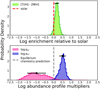 |
Fig. 12 Ratio of the titanium metallicity relative to the overall metallicity (green distribution, cross marker) as well as the hydride (blue distribution, squared marker) and free electron (red distribution, dotted marker) abundance multipliers retrieved from the joint HARPS + NIRPS retrieval. The top panel shows the enrichment relative to solar (red dashed line) in logarithmic scale for titanium. The bottom panel shows the abundance profile for H− (bound-free) and free electrons multipliers as predicted by chemical equilibrium chemistry with FastChem. Here we see that the H− (bound-free) retrieved abundance is about 0.5 dex higher than that of the metals, as predicted by equilibrium chemistry (grey dashed line). This indicates that, while species such as Fe have very strong lines in the optical, others that only have weaker spectral features may be harder to detect with transmission spectroscopy on ultra-hot Jupiters like WASP-189b. The error bars, which are shown as black markers, were calculated as the standard deviation around the median value of each distribution. |
Acknowledgements
This work has been carried out within the framework of the NCCR PlanetS supported by the Swiss National Science Foundation under grants 51NF40_182901 and 51NF40_205606.VV, DE acknowledge support from the Swiss National Science Foundation for project 200021_200726. The authors acknowledge the financial support of the SNSF.RA acknowledges the Swiss National Science Foundation (SNSF) support under the Post-Doc Mobility grant P500PT_222212 and the support of the Institut Trottier de Recherche sur les Exoplanètes (IREx).RA, ÉA, FBa, BB, RD, LMa, LB, CC, NJC, LD, AL & TV acknowledge the financial support of the FRQ-NT through the Centre de recherche en astrophysique du Québec as well as the support from the Trottier Family Foundation and the Trottier Institute for Research on Exoplanets.EC, SCB, ED-M, NCS, ARCS & JGd acknowledge the support from FCT – Fundação para a Ciência e a Tecnologia through national funds by these grants: UIDB/04434/2020, UIDP/04434/2020.XDu acknowledges the support from the European Research Council (ERC) under the European Union’s Horizon 2020 research and innovation programme (grant agreement SCORE No. 851555) and from the Swiss National Science Foundation under the grant SPECTRE (No. 200021_215200).HC, ML & BA acknowledge support of the Swiss National Science Foundation under grant number PCEFP2_194576.ÉA, FBa, RD & LMa acknowledges support from Canada Foundation for Innovation (CFI) program, the Université de Montréal and Université Laval, the Canada Economic Development (CED) program and the Ministere of Economy, Innovation and Energy (MEIE).SCB acknowledges the support from Fundação para a Ciência e Tecnologia (FCT) in the form of work of work through the Scientific Employment Incentive program (reference 2023.06687.CEECIND).XB and JMA acknowledge funding from the European Research Council under the ERC Grant Agreement no. 337591-ExTrA.XB, XDe, TF & VY acknowledge funding from the French ANR under contract number ANR18CE310019 (SPlaSH), and the French National Research Agency in the framework of the Investissements d’Avenir program (ANR-15-IDEX-02), through the funding of the “Origin of Life” project of the Grenoble-Alpes University.The Board of Observational and Instrumental Astronomy (NAOS) at the Federal University of Rio Grande do Norte’s research activities are supported by continuous grants from the Brazilian funding agency CNPq. This study was partially funded by the Coordenação de Aperfeiçoamento de Pessoal de Nível Superior-Brasil (CAPES) – Finance Code 001 and the CAPES-Print program.BLCM acknowledge CAPES postdoctoral fellowships.BLCM acknowledges CNPq research fellowships (Grant No. 305804/2022-7).NBC acknowledges support from an NSERC Discovery Grant, a Canada Research Chair, and an Arthur B. McDonald Fellowship, and thanks the Trottier Space Institute for its financial support and dynamic intellectual environment.JRM acknowledges CNPq research fellowships (Grant No. 308928/2019-9).ED-M further acknowledges the support from FCT through Stimulus FCT contract 2021.01294.CEECIND. ED-M acknowledges the support by the Ramón y Cajal grant RyC2022-035854-I funded by MICIU/AEI/10.13039/50110001103 and by ESF+.JIGH, RR, ASM, NN & AKS acknowledge financial support from the Spanish Ministry of Science, Innovation and Universities (MICIU) projects PID2020-117493GB-I00 and PID2023-149982NB-I00.ICL acknowledges CNPq research fellowships (Grant No. 313103/2022-4).CMo acknowledges the funding from the Swiss National Science Foundation under grant 200021_204847 “PlanetsInTime”.Co-funded by the European Union (ERC, FIERCE, 101052347). Views and opinions expressed are however those of the author(s) only and do not necessarily reflect those of the European Union or the European Research Council. Neither the European Union nor the granting authority can be held responsible for them. This project has received funding from the European Research Council (ERC) under the European Union’s Horizon 2020 research and innovation programme (project SPICE Dune, grant agreement No. 947634). This material reflects only the authors’ views and the Commission is not liable for any use that may be made of the information contained therein.ARCS acknowledges the support from Fundaçao para a Ciência e a Tecnologia (FCT) through the fellowship 2021.07856.BD.LD acknowledges the support of the Natural Sciences and Engineering Research Council of Canada (NSERC) [funding reference number 521489] and from the Fonds de recherche du Québec (FRQ) – Secteur Nature et technologies [funding file number 332355].RLG acknowledge CAPES graduate fellowships.FG acknowledges support from the Fonds de recherche du Québec (FRQ) – Secteur Nature et technologies under file #350366.AL acknowledges support from the Fonds de recherche du Québec (FRQ) – Secteur Nature et technologies under file #349961.NN acknowledges financial support by Light Bridges S.L, Las Palmas de Gran Canaria.NN acknowledges funding from Light Bridges for the Doctoral Thesis “Habitable Earth-like planets with ESPRESSO and NIRPS”, in cooperation with the Instituto de Astrofísica de Canarias, and the use of Indefeasible Computer Rights (ICR) being commissioned at the ASTRO POC project in the Island of Tenerife, Canary Islands (Spain). The ICR-ASTRONOMY used for his research was provided by Light Bridges in cooperation with Hewlett Packard Enterprise (HPE).AP acknowledges support from the Unidad de Excelencia María de Maeztu CEX2020-001058-M programme and from the Generalitat de Catalunya/CERCA.AKS acknowledges financial support from La Caixa Foundation (ID 100010434) under the grant LCF/BQ/DI23/11990071.TV acknowledges support from the Fonds de recherche du Québec (FRQ) – Secteur Nature et technologies under file #320056.
Appendix A CONAN prior and posterior distribution
CONAN prior and posterior distribution.
Appendix B Gaussian fitting to the Doppler shadow
Initial guesses as to Gaussian fitting.
Appendix C Hydrogen lines in the transit spectrum of WASP-189b
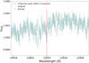 |
Fig. C.1 Transmission spectrum of WASP-189b around the hydrogen Paschen-β line (dashed red line). No evidences of hydrogen spectral lines belonging to the Paschen series. |
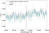 |
Fig. C.2 Transmission spectrum of WASP-189b around the hydrogen Paschen-γ line (dashed red line). No evidences of hydrogen spectral lines belonging to the Paschen series. |
Appendix D SCARLET atmospheric modelled spectra of WASP-189b
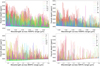 |
Fig. D.1 Full resolution SCARLET synthetic spectra of the atmosphere of WASP-189b for all the chemical species of interest (details in Section 5.2). Top and bottom panels show all the atomic species in the HARPS and NIRPS coverage, respectively. |
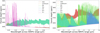 |
Fig. D.2 Full resolution SCARLET synthetic spectra of the atmosphere of WASP-189b for all the chemical species of interest (details in Section 5.2). Left and right panels show the molecular and ionic species in the HARPS and NIRPS coverage, respectively. |
Appendix E Comparison between different telluric correction methods
We conduct additional tests to evaluate the quality of the telluric correction applied to near-infrared NIRPS data. Specifically, we compare the telluric correction performed using the molecfit tool against that implemented by the instrument’s automated DRS 3.2.0 based on Allart et al. (2022). To obtain a cleaner cross-correlation map for H2O out of the DRS telluric corrected NIRPS data, we increase the filtering percentage. Despite the improvements, both water cross-correlation maps (focused on the second WASP-189b transit happened on 2023-06-04, top and central panels in Figure E.1) still display residuals (as vertical stripes) highlighting that neither molecfit nor the DRS 3.2.0 correction are able to suppress telluric lines to a sufficient level. With remaining residuals at a greater level than the planetary signal, it is certain that this would bias inferred parameters from an atmospheric retrieval. In comparison, we find that the PCA method (see the bottom panel in Figure E.1) is more effective at cleaning the data of water residuals. The persistence of telluric remnants above a comfortable level, even after processing NIRPS data with the DRS pipeline or correction using molecfit, inevitably guarantees contamination by water telluric residuals. Therefore, we proceed with the alternative PCA approach to clean NIRPS data, before they are digested by the atmospheric retrieval. The following cross-correlation trail maps for H2O are useful tovisualise how different telluric correction approaches behave applied to near-infrared NIRPS data.
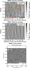 |
Fig. E.1 Top panel: Cross-correlation trail map for H2O out of molecfit telluric corrected NIRPS data and a 90% filtering. Central panel: Cross-correlation trail map for H2O out of DRS telluric corrected NIRPS data and a 90% filtering (see Sec. 4 and 5.1.2 for a detailed description of the data analysis process). Bottom panel: Cross-correlation trail map for H2O out of PCA corrected NIRPS data. |
Appendix F HARPS negative injection test
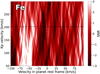 |
Fig. F.1 Kp–vsys showcasing how the atomic Fe signal detected in HARPS data was cancelled out by the negative injection (in emission) of the fiducial model. This probe that the model used matches well the amplitude of the real signal (details in Section 5.2.2). Peaks at ~−50 and +50 km s−1 are artefacts of the Rossiter-McLaughlin correction. |
Appendix G NIRPS non-detections in the transit spectrum of WASP-189b
Line-contrast upper limits calculated for non-detections of listed neutral chemical species in the NIRPS transmission spectrum of WASP-189b.
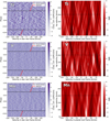 |
Fig. G.1 NIRPS cross-correlation results showing non-detected chemical species. Black dashed lines (right panel) denote the expected Kp determined from Prinoth et al. (2023), and vsys = 0 km s−1. Left column: cross-correlation trail map. Right column: cross-correlation Kp–vsys map. |
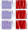 |
Fig. G.5 NIRPS non-detections, G.1 continued. Remnants of the telluric correction (beyond and within in-transit phases) are visible in the water and OH cross-correlation maps. |
Appendix H HARPS non-detections in the transit spectrum of WASP-189b
Line-contrast upper limits calculated for non-detections of listed chemical species in the HARPS transmission spectrum of WASP-189b.
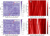 |
Fig. H.1 HARPS cross-correlation results showing non-detected chemical species. |
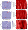 |
Fig. H.4 HARPS non-detections, H.1 continued. The cross-correlation maps for H2O present features around 25 km s−1 due to remnant artefacts of the telluric correction. |
Appendix I PCA-based CCF analysis
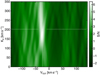 |
Fig. I.1 Cross-correlation detection of Fe from the HARPS transits, but now using a blind data-driven PCA-based detrending algorithm instead. The white dashed lines denote the expected Kp and vsys (Kp=200.7 km s−1 and vsys=−24.45 km s−1; Prinoth et al. 2022; Anderson et al. 2018) of WASP-189b assuming a uniform and static atmosphere. The white blob near the expected location shows the observed signal of WASP-189b. Differently from Figure 6, 7, 8, and, H.1, G.1, this map has been generated from transmission spectra non-shifted by the systemic velocity. The uniformness of the CCF map between 0 and 50 km s−1 at low Kp values is a result of the Rossiter-McLaughlin mask excluding values overlapping with the Doppler shadow in radial velocity space. The data product that produced this CCF map is the input for the atmospheric retrieval analysis (Section 5.3). |
References
- Allart, R., Lovis, C., Pino, L., et al. 2017, A&A, 606, A144 [NASA ADS] [CrossRef] [EDP Sciences] [Google Scholar]
- Allart, R., Bourrier, V., Lovis, C., et al. 2018, Science, 362, 1384 [Google Scholar]
- Allart, R., Lovis, C., Faria, J., et al. 2022, A&A, 666, A196 [NASA ADS] [CrossRef] [EDP Sciences] [Google Scholar]
- Allart, R., Lemée-Joliecoeur, P. B., Jaziri, A. Y., et al. 2023, A&A, 677, A164 [NASA ADS] [CrossRef] [EDP Sciences] [Google Scholar]
- Allart, R., Carteret, Y., Bourrier, V., et al. 2025, A&A, 700, A7 [NASA ADS] [CrossRef] [EDP Sciences] [Google Scholar]
- Anderson, D. R., Temple, L. Y., Nielsen, L. D., et al. 2018, arXiv e-prints [arXiv:1809.04897] [Google Scholar]
- Arcangeli, J., Désert, J.-M., Line, M. R., et al. 2018, ApJ, 855, L30 [Google Scholar]
- Arcangeli, J., Désert, J.-M., Parmentier, V., et al. 2019, A&A, 625, A136 [NASA ADS] [CrossRef] [EDP Sciences] [Google Scholar]
- Asplund, M., Grevesse, N., Sauval, A. J., & Scott, P. 2009, Annu. Rev. Astron. Astrophys., 47, 481 [CrossRef] [Google Scholar]
- Bazinet, L., Pelletier, S., Benneke, B., Salinas, R., & Mace, G. N. 2024, AJ, 167, 206 [NASA ADS] [CrossRef] [Google Scholar]
- Bell, T. J., & Cowan, N. B. 2018, ApJ, 857, L20 [Google Scholar]
- Benneke, B. 2015, arXiv e-prints [arXiv:1504.07655] [Google Scholar]
- Benneke, B., & Seager, S. 2012, ApJ, 753, 100 [NASA ADS] [CrossRef] [Google Scholar]
- Benneke, B., & Seager, S. 2013, ApJ, 778, 153 [Google Scholar]
- Benneke, B., Knutson, H. A., Lothringer, J., et al. 2019, Nat.. Astron., 3, 813 [Google Scholar]
- Benz, W., Broeg, C., Fortier, A., et al. 2021, Exp. Astron., 51, 109 [Google Scholar]
- Bonfils, X., Almenara, J. M., Jocou, L., et al. 2015, SPIE Conf. Ser., 9605, 96051L [NASA ADS] [Google Scholar]
- Borsa, F., Allart, R., Casasayas-Barris, N., et al. 2021, A&A, 645, A24 [EDP Sciences] [Google Scholar]
- Bouchy, F., Doyon, R., Artigau, É., et al. 2017, The Messenger, 169, 21 [NASA ADS] [Google Scholar]
- Bouchy, F., Doyon, R., Pepe, F., et al. 2025, A&A, 700, A10 [NASA ADS] [CrossRef] [EDP Sciences] [Google Scholar]
- Brogi, M., & Line, M. R. 2019, AJ, 157, 114 [Google Scholar]
- Brogi, M., Snellen, I. A. G., de Kok, R. J., et al. 2012, Nature, 486, 502 [Google Scholar]
- Brown, T. M. 2001, ApJ, 553, 1006 [NASA ADS] [CrossRef] [Google Scholar]
- Casasayas-Barris, N., Borsa, F., Palle, E., et al. 2022, A&A, 664, A121 [NASA ADS] [CrossRef] [EDP Sciences] [Google Scholar]
- Cheverall, C. J., & Madhusudhan, N. 2024, AJ, 167, 272 [NASA ADS] [CrossRef] [Google Scholar]
- Claudi, R., Benatti, S., Carleo, I., et al. 2017, Eur. Phys. J. Plus, 132, 364 [NASA ADS] [CrossRef] [Google Scholar]
- Collier Cameron, A., Guenther, E., Smalley, B., et al. 2010, MNRAS, 407, 507 [NASA ADS] [CrossRef] [Google Scholar]
- Cook, N. J., Artigau, E., Doyon, R., et al. 2022, PASP, 134, 114509 [NASA ADS] [CrossRef] [Google Scholar]
- Cosentino, R., Lovis, C., Pepe, F., et al. 2012, SPIE Conf. Ser., 8446, 84461V [Google Scholar]
- Cowley, A. P. 1968, PASP, 80, 453 [Google Scholar]
- Deline, A., Hooton, M. J., Lendl, M., et al. 2022, A&A, 659, A74 [NASA ADS] [CrossRef] [EDP Sciences] [Google Scholar]
- Delrez, L., Santerne, A., Almenara, J. M., et al. 2016, MNRAS, 458, 4025 [NASA ADS] [CrossRef] [Google Scholar]
- Ehrenreich, D., Lovis, C., Allart, R., et al. 2020, Nature, 580, 597 [Google Scholar]
- Espinoza, N., & Jordán, A. 2015, MNRAS, 450, 1879 [Google Scholar]
- Evans, T. M., Sing, D. K., Kataria, T., et al. 2017, Nature, 548, 58 [NASA ADS] [CrossRef] [Google Scholar]
- Foreman-Mackey, D., Hogg, D. W., Lang, D., & Goodman, J. 2013, PASP, 125, 306 [Google Scholar]
- France, K., Fleming, B., Egan, A., et al. 2023, AJ, 165, 63 [Google Scholar]
- Galland, F., Lagrange, A. M., Udry, S., et al. 2005, A&A, 443, 337 [NASA ADS] [CrossRef] [EDP Sciences] [Google Scholar]
- Gandhi, S., Kesseli, A., Zhang, Y., et al. 2023, AJ, 165, 242 [NASA ADS] [CrossRef] [Google Scholar]
- Gaudi, B. S., Stassun, K. G., Collins, K. A., et al. 2017, Nature, 546, 514 [NASA ADS] [Google Scholar]
- Gibson, N. P., Merritt, S., Nugroho, S. K., et al. 2020, MNRAS, 493, 2215 [Google Scholar]
- Gibson, N. P., Nugroho, S. K., Lothringer, J., Maguire, C., & Sing, D. K. 2022, MNRAS, 512, 4618 [NASA ADS] [CrossRef] [Google Scholar]
- Gray, D. F. 2021, The Observation and Analysis of Stellar Photospheres, 4th edn. (Cambridge University Press) [Google Scholar]
- Grimm, S. L., & Heng, K. 2015, ApJ, 808, 182 [NASA ADS] [CrossRef] [Google Scholar]
- Grimm, S. L., Malik, M., Kitzmann, D., et al. 2021, ApJS, 253, 30 [NASA ADS] [CrossRef] [Google Scholar]
- Hellier, C., Anderson, D. R., Collier Cameron, A., et al. 2009, Nature, 460, 1098 [NASA ADS] [CrossRef] [Google Scholar]
- Helling, C., Lewis, D., Samra, D., et al. 2021, A&A, 649, A44 [NASA ADS] [CrossRef] [EDP Sciences] [Google Scholar]
- Hoeijmakers, H. J., Ehrenreich, D., Heng, K., et al. 2018, Nature, 560, 453 [CrossRef] [Google Scholar]
- Hoeijmakers, H. J., Ehrenreich, D., Kitzmann, D., et al. 2019, A&A, 627, A165 [NASA ADS] [CrossRef] [EDP Sciences] [Google Scholar]
- Hoeijmakers, H. J., Seidel, J. V., Pino, L., et al. 2020, A&A, 641, A123 [NASA ADS] [CrossRef] [EDP Sciences] [Google Scholar]
- Hoeijmakers, H. J., Kitzmann, D., Morris, B. M., et al. 2024, A&A, 685, A139 [NASA ADS] [CrossRef] [EDP Sciences] [Google Scholar]
- Husser, T. O., Wende-von Berg, S., Dreizler, S., et al. 2013, A&A, 553, A6 [NASA ADS] [CrossRef] [EDP Sciences] [Google Scholar]
- Kausch, W., Noll, S., Smette, A., et al. 2015, A&A, 576, A78 [NASA ADS] [CrossRef] [EDP Sciences] [Google Scholar]
- Kesseli, A. Y., Snellen, I. A. G., Casasayas-Barris, N., Mollière, P., & SánchezLópez, A. 2022, AJ, 163, 107 [NASA ADS] [CrossRef] [Google Scholar]
- Kitzmann, D., Heng, K., Rimmer, P. B., et al. 2018, ApJ, 863, 183 [Google Scholar]
- Komacek, T. D., Tan, X., Gao, P., & Lee, E. K. H. 2022, ApJ, 934, 79 [NASA ADS] [CrossRef] [Google Scholar]
- Kurucz, R. L. 1979, ApJS, 40, 1 [NASA ADS] [CrossRef] [Google Scholar]
- Lendl, M., Anderson, D. R., Collier-Cameron, A., et al. 2012, A&A, 544, A72 [NASA ADS] [CrossRef] [EDP Sciences] [Google Scholar]
- Lendl, M., Cubillos, P. E., Hagelberg, J., et al. 2017, A&A, 606, A18 [NASA ADS] [CrossRef] [EDP Sciences] [Google Scholar]
- Lendl, M., Csizmadia, S., Deline, A., et al. 2020, A&A, 643, A94 [EDP Sciences] [Google Scholar]
- Lesjak, F., Nortmann, L., Cont, D., et al. 2025, A&A, 693, A72 [NASA ADS] [CrossRef] [EDP Sciences] [Google Scholar]
- Li, G., Gordon, I. E., Rothman, L. S., et al. 2015, ApJS, 216, 15 [NASA ADS] [CrossRef] [Google Scholar]
- Lothringer, J. D., Barman, T., & Koskinen, T. 2018, ApJ, 866, 27 [NASA ADS] [CrossRef] [Google Scholar]
- Lund, M. B., Rodriguez, J. E., Zhou, G., et al. 2017, AJ, 154, 194 [Google Scholar]
- Maguire, C., Gibson, N. P., Nugroho, S. K., et al. 2023, MNRAS, 519, 1030 [Google Scholar]
- Mayor, M., Pepe, F., Queloz, D., et al. 2003, The Messenger, 114, 20 [NASA ADS] [Google Scholar]
- McKemmish, L. K., Masseron, T., Hoeijmakers, H. J., et al. 2019, MNRAS, 488, 2836 [Google Scholar]
- McLaughlin, D. B. 1924, ApJ, 60, 22 [Google Scholar]
- Merritt, S. R., Gibson, N. P., Nugroho, S. K., et al. 2020, A&A, 636, A117 [NASA ADS] [CrossRef] [EDP Sciences] [Google Scholar]
- Mounzer, D., Lovis, C., Seidel, J. V., et al. 2022, A&A, 668, A1 [NASA ADS] [CrossRef] [EDP Sciences] [Google Scholar]
- Nortmann, L., Pallé, E., Salz, M., et al. 2018, Science, 362, 1388 [Google Scholar]
- Oklopčić, A., & Hirata, C. M. 2018, ApJ, 855, L11 [Google Scholar]
- Parmentier, V., Line, M. R., Bean, J. L., et al. 2018, A&A, 617, A110 [NASA ADS] [CrossRef] [EDP Sciences] [Google Scholar]
- Pelletier, S., Benneke, B., Darveau-Bernier, A., et al. 2021, AJ, 162, 73 [NASA ADS] [CrossRef] [Google Scholar]
- Pelletier, S., Benneke, B., Ali-Dib, M., et al. 2023, Nature, 619, 491 [NASA ADS] [CrossRef] [Google Scholar]
- Pelletier, S., Benneke, B., Chachan, Y., et al. 2024, AJ, 169, 10 [Google Scholar]
- Pepe, F., Cristiani, S., Rebolo, R., et al. 2021, A&A, 645, A96 [NASA ADS] [CrossRef] [EDP Sciences] [Google Scholar]
- Pluriel, W., Whiteford, N., Edwards, B., et al. 2020, AJ, 160, 112 [NASA ADS] [CrossRef] [Google Scholar]
- Polyansky, O. L., Kyuberis, A. A., Zobov, N. F., et al. 2018, MNRAS, 480, 2597 [NASA ADS] [CrossRef] [Google Scholar]
- Prinoth, B., Hoeijmakers, H. J., Kitzmann, D., et al. 2022, Nat. Astron., 6, 449 [NASA ADS] [CrossRef] [Google Scholar]
- Prinoth, B., Hoeijmakers, H. J., Pelletier, S., et al. 2023, A&A, 678, A182 [NASA ADS] [CrossRef] [EDP Sciences] [Google Scholar]
- Prinoth, B., Hoeijmakers, H. J., Morris, B. M., et al. 2024, A&A, 685, A60 [NASA ADS] [CrossRef] [EDP Sciences] [Google Scholar]
- Renson, P., & Manfroid, J. 2009, A&A, 498, 961 [NASA ADS] [CrossRef] [EDP Sciences] [Google Scholar]
- Rodgers, J., & Nicewander, A. 1988, Amer. Statist., 42, 59 [Google Scholar]
- Rossiter, R. A. 1924, ApJ, 60, 15 [Google Scholar]
- Rothman, L. S., Gordon, I. E., Barber, R. J., et al. 2010, JQSRT, 111, 2139 [NASA ADS] [CrossRef] [Google Scholar]
- Rousselot, P., Lidman, C., Cuby, J. G., Moreels, G., & Monnet, G. 2000, A&A, 354, 1134 [Google Scholar]
- Ryabchikova, T., Piskunov, N., Kurucz, R. L., et al. 2015, Phys. Scr., 90, 054005 [Google Scholar]
- Saffe, C., Miquelarena, P., Alacoria, J., et al. 2021, A&A, 647, A49 [NASA ADS] [CrossRef] [EDP Sciences] [Google Scholar]
- Saffe, C., Alacoria, J., Miquelarena, P., et al. 2022, A&A, 668, A157 [NASA ADS] [CrossRef] [EDP Sciences] [Google Scholar]
- Salz, M., Czesla, S., Schneider, P. C., et al. 2018, A&A, 620, A97 [NASA ADS] [CrossRef] [EDP Sciences] [Google Scholar]
- Sánchez-López, A., Lin, L., Snellen, I. A. G., et al. 2022, A&A, 666, L1 [NASA ADS] [CrossRef] [EDP Sciences] [Google Scholar]
- Seager, S., & Sasselov, D. D. 2000, ApJ, 537, 916 [Google Scholar]
- Seidel, J. V., Ehrenreich, D., Wyttenbach, A., et al. 2019, A&A, 623, A166 [NASA ADS] [CrossRef] [EDP Sciences] [Google Scholar]
- Seidel, J. V., Ehrenreich, D., Bourrier, V., et al. 2020, A&A, 641, L7 [NASA ADS] [CrossRef] [EDP Sciences] [Google Scholar]
- Seidel, J. V., Ehrenreich, D., Allart, R., et al. 2021, A&A, 653, A73 [NASA ADS] [CrossRef] [EDP Sciences] [Google Scholar]
- Seidel, J. V., Borsa, F., Pino, L., et al. 2023, A&A, 673, A125 [NASA ADS] [CrossRef] [EDP Sciences] [Google Scholar]
- Seifahrt, A., Stürmer, J., Bean, J. L., & Schwab, C. 2018, SPIE Conf. Ser., 10702, 107026D [NASA ADS] [Google Scholar]
- Seifahrt, A., Bean, J. L., Stürmer, J., et al. 2020, SPIE Conf. Ser., 11447, 114471F [NASA ADS] [Google Scholar]
- Sing, D. K., Fortney, J. J., Nikolov, N., et al. 2016, Nature, 529, 59 [Google Scholar]
- Skrutskie, M. F., Cutri, R. M., Stiening, R., et al. 2006, AJ, 131, 1163 [NASA ADS] [CrossRef] [Google Scholar]
- Smette, A., Sana, H., Noll, S., et al. 2015, A&A, 576, A77 [NASA ADS] [CrossRef] [EDP Sciences] [Google Scholar]
- Snellen, I. A. G., de Kok, R. J., de Mooij, E. J. W., & Albrecht, S. 2010, Nature, 465, 1049 [Google Scholar]
- Spake, J. J., Sing, D. K., Evans, T. M., et al. 2018, Nature, 557, 68 [Google Scholar]
- Sreejith, A. G., France, K., Fossati, L., et al. 2023, ApJ, 954, L23 [NASA ADS] [CrossRef] [Google Scholar]
- Stangret, M., Casasayas-Barris, N., Pallé, E., et al. 2022, A&A, 662, A101 [NASA ADS] [CrossRef] [EDP Sciences] [Google Scholar]
- Stock, J. W., Kitzmann, D., Patzer, A. B. C., & Sedlmayr, E. 2018, MNRAS, 479, 865 [NASA ADS] [Google Scholar]
- Stock, J. W., Kitzmann, D., & Patzer, A. B. C. 2022, MNRAS, 517, 4070 [NASA ADS] [CrossRef] [Google Scholar]
- Talens, G. J. J., Justesen, A. B., Albrecht, S., et al. 2018, A&A, 612, A57 [NASA ADS] [CrossRef] [EDP Sciences] [Google Scholar]
- Wardenier, J. P., Parmentier, V., Lee, E. K. H., Line, M. R., & Gharib-Nezhad, E. 2021, MNRAS, 506, 1258 [NASA ADS] [CrossRef] [Google Scholar]
- Wardenier, J. P., Parmentier, V., Line, M. R., & Lee, E. K. H. 2023, MNRAS, 525, 4942 [NASA ADS] [CrossRef] [Google Scholar]
- West, R. G., Hellier, C., Almenara, J. M., et al. 2016, A&A, 585, A126 [NASA ADS] [CrossRef] [EDP Sciences] [Google Scholar]
- Wildi, F., Bouchy, F., Doyon, R., et al. 2022, in Ground-based and Airborne Instrumentation for Astronomy IX, 12184, eds. C. J. Evans, J. J. Bryant, & K. Motohara, International Society for Optics and Photonics (SPIE), 121841H [Google Scholar]
- Wildt, R. 1939, ApJ, 90, 611 [NASA ADS] [CrossRef] [Google Scholar]
- Wong, I., Shporer, A., Zhou, G., et al. 2021, AJ, 162, 256 [NASA ADS] [CrossRef] [Google Scholar]
- Wyttenbach, A., Ehrenreich, D., Lovis, C., Udry, S., & Pepe, F. 2015, A&A, 577, A62 [NASA ADS] [CrossRef] [EDP Sciences] [Google Scholar]
- Wyttenbach, A., Mollière, P., Ehrenreich, D., et al. 2020, A&A, 638, A87 [EDP Sciences] [Google Scholar]
- Yan, F., & Henning, T. 2018, Nat. Astron., 2, 714 [Google Scholar]
- Yan, F., Pallé, E., Reiners, A., et al. 2020, A&A, 640, L5 [NASA ADS] [CrossRef] [EDP Sciences] [Google Scholar]
- Yan, F., Pallé, E., Reiners, A., et al. 2022, A&A, 661, L6 [NASA ADS] [CrossRef] [EDP Sciences] [Google Scholar]
It is worth mentioning a second reduction pipeline, APERO (A PipelinE to Reduce Observations, Cook et al. 2022) to process near-infrared NIRPS data. The spectra reduced by APERO are fully consistent with those produced by the ESPRESSO pipeline.
![$\[\sigma_{K_{p}}= K_{p} \times \sqrt{\left(\frac{1}{3} \frac{\sigma_{M_{\star}}}{M_{\star}}\right)^{2}+\left(\frac{1}{3} \frac{P}{\sigma_{P}}\right)^{2}}\]$](/articles/aa/full_html/2025/08/aa52972-24/aa52972-24-eq35.png)
All Tables
WASP-189b SCARLET atmospheric posteriors from the retrieval analysis on the HARPS and NIRPS time series combined.
Line-contrast upper limits calculated for non-detections of listed neutral chemical species in the NIRPS transmission spectrum of WASP-189b.
Line-contrast upper limits calculated for non-detections of listed chemical species in the HARPS transmission spectrum of WASP-189b.
All Figures
|
Fig. 1 Observing conditions during Night 1 and Night 2 as a function of phase (phase = (BJD − Tc)/P, where BJD is the barycentric Julian date, Tc = 2458926.5 days is the mid-transit time, and P = 2.724033 days is the period, which are all from Lendl et al. 2020). The top panel and mid panel illustrate the airmass and the average atmospheric Dimm seeing evolving during the nights, respectively. The Dimm seeing is averaged for each observations (i.e. average between the start and the end of each observation). The bottom panel shows the S/N (extracted from the fits header) changing during the nights. |
| In the text | |
|
Fig. 2 De-trended light curve obtained with ExTrA and EulerCam, respectively. The transit model is over-plotted in red. The root-mean-squares of EulerCam and ExTrA light curves are 1206 and 1620 ppm, respectively. |
| In the text | |
|
Fig. 3 One-dimensional cross-correlation function based on HARPS data calculated for neutral iron before (orange) and after (blue) correcting for the stellar contamination in the form of the two-component Rossiter-McLaughlin effect. |
| In the text | |
|
Fig. 4 Cross-correlation map based on HARPS data with no correction of the Rossiter-McLaughlin effect. The top panel shows the pre-correction scenario. The thick emitting dark vertical strip around 50 km s−1 is the first component of the Rossiter-McLaughlin contamination, that is called Doppler shadow. The wide absorbing feature from ~−80 km s−1 up to ~25 km s−1 is the second component of the stellar contamination. Bottom panel: the post-correction scenario once the best Gaussian fits are subtracted from the cross-correlation. |
| In the text | |
|
Fig. 5 Transmission spectrum of WASP-189b around the metastable helium triplet (vertical dashed red lines). Grey dots with error bars represent the entire transmission spectrum at native resolution, and cyan dots with uncertainties are the binned spectrum. No trace of metastable helium triplet is found in WASP-189b from atomic line inspection of its transmission spectrum, as expected given the theory of Oklopčić & Hirata (2018). |
| In the text | |
|
Fig. 6 Neutral Fe cross-correlation from two transits of WASP-189b observed with the HARPS spectrograph. Left panel: cross-correlation time series corrected for the Rossiter–McLauglin contribution. The planetary trail follows the Keplerian motion in red, and it is bound within the transit window (first and fourth contact transit phases indicated by horizontal black dashed line). Right panel: Kp−vsys diagram. The black dashed lines denote the expected vsys and Kp from Prinoth et al. (2023). The region enclosed in the cyan dotted box is used for the calculation of the S/N used throughout the entire map. Features around +50 and −50 km/s are residuals of the Rossiter-McLaughlin correction fitting and not due statistical fluctuations (Section 4.3.1). |
| In the text | |
|
Fig. 7 Left panel: maximum S/N versus velocities at the measured Kp (blue curve). In red, the best-fit Gaussian to the Fe cross-correlation peak, whose centroid results blueshifted by −5.54 ± 0.44 km/s with respect to zero km/s. The positive peaks around ~40 km s−1, ~−60 km s−1, and the negative peak at ~−20 km s−1 are artefacts of the Rossiter-McLaughlin correction and not statistical fluctuations. Right panel: ΔKp−vsys diagram. The ΔKp is calculated as ΔKp = Kp − Kp,measured (Wardenier et al. 2023). The black dashed lines denote the expected vsys and Kp from Prinoth et al. (2023) (i.e. Kp = 200.7 km s−1). Features around +50 and −50 km/s are residuals of the Rossiter-McLaughlin correction fitting and not due statistical fluctuations (Section 4.3.1). |
| In the text | |
|
Fig. 8 Cross-correlation trail map (left panel) and Kp–vsys map (right panel) of NIRPS data, obtained with the reduction pipeline described in Section 4. Black dashed lines (right panel) denote the expected Kp determined from Prinoth et al. (2023), and vsys=0 km s−1. The colourmaps show a non-detection of Fe from two transits of WASP-189b observed with the NIRPS spectrograph. The observation gap occurred during the first transit on the night of 2023-04-24 is visible as a banded structure of higher scatter between phases 0.0 and 0.02 (left panel). |
| In the text | |
|
Fig. 9 Iron atmospheric model spectrum as a function of wavelength including contributions given by the hydride as a source of continuum absorption. In blue the atmospheric model for Fe, with no absorber added. In orange, the template spectrum including H− free-free as source of continuum opacity, boosted by a factor of 10. In red, the spectrum including a solar amount of H− bound-free. In the green and purple spectra, the bound-free contribution is boosted by a factor of 10 and 1000, respectively. The purple spectrum includes contributions by H2O beyond 1.6 μm. The grey and cyan coloured regions indicate HARPS and NIRPS coverage, respectively. It is worth mentioning that HARPS and NIRPS cover a similar fractional bandpass. We intentionally boost the continuum level differentiating the two main contributions to illustrate how the Fe spectrum changes accordingly. |
| In the text | |
|
Fig. 10 Kp–vsys map showcasing the injection-recovery test on NIRPS data. Left panel: the injected iron atmospheric model includes contributions from the H− as a source of continuum opacity; the map shows no detection of atomic Fe in the near-infrared data of WASP-189b, consistent with non-injected results. Right panel: the injected iron atmospheric model does not include contributions from the hydride; in this case, the map shows a clear detection of neutral Fe in the near-infrared data. Black dashed lines denote the expected vsys and Kp determined from Prinoth et al. (2023). |
| In the text | |
|
Fig. 11 Retrieved constraints on the atmospheric and orbital properties obtained from the observed two transits of WASP-189b. The orange shows the retrieval considering only the HARPS data, while the blue shows with the inclusion of NIRPS. Here the overall metallicity, as well as the titanium-only metallicity are well constrained to be near-solar. Meanwhile the H− abundance is slightly above expectations from solar model in chemical equilibrium. The inclusion of the NIRPS data is particularly helpful in constraining the H− abundance, as well as setting a strict upper limit on the free electron density, which is unconstrained from the HARPS-only retrieval. |
| In the text | |
|
Fig. 12 Ratio of the titanium metallicity relative to the overall metallicity (green distribution, cross marker) as well as the hydride (blue distribution, squared marker) and free electron (red distribution, dotted marker) abundance multipliers retrieved from the joint HARPS + NIRPS retrieval. The top panel shows the enrichment relative to solar (red dashed line) in logarithmic scale for titanium. The bottom panel shows the abundance profile for H− (bound-free) and free electrons multipliers as predicted by chemical equilibrium chemistry with FastChem. Here we see that the H− (bound-free) retrieved abundance is about 0.5 dex higher than that of the metals, as predicted by equilibrium chemistry (grey dashed line). This indicates that, while species such as Fe have very strong lines in the optical, others that only have weaker spectral features may be harder to detect with transmission spectroscopy on ultra-hot Jupiters like WASP-189b. The error bars, which are shown as black markers, were calculated as the standard deviation around the median value of each distribution. |
| In the text | |
|
Fig. C.1 Transmission spectrum of WASP-189b around the hydrogen Paschen-β line (dashed red line). No evidences of hydrogen spectral lines belonging to the Paschen series. |
| In the text | |
|
Fig. C.2 Transmission spectrum of WASP-189b around the hydrogen Paschen-γ line (dashed red line). No evidences of hydrogen spectral lines belonging to the Paschen series. |
| In the text | |
|
Fig. D.1 Full resolution SCARLET synthetic spectra of the atmosphere of WASP-189b for all the chemical species of interest (details in Section 5.2). Top and bottom panels show all the atomic species in the HARPS and NIRPS coverage, respectively. |
| In the text | |
|
Fig. D.2 Full resolution SCARLET synthetic spectra of the atmosphere of WASP-189b for all the chemical species of interest (details in Section 5.2). Left and right panels show the molecular and ionic species in the HARPS and NIRPS coverage, respectively. |
| In the text | |
|
Fig. E.1 Top panel: Cross-correlation trail map for H2O out of molecfit telluric corrected NIRPS data and a 90% filtering. Central panel: Cross-correlation trail map for H2O out of DRS telluric corrected NIRPS data and a 90% filtering (see Sec. 4 and 5.1.2 for a detailed description of the data analysis process). Bottom panel: Cross-correlation trail map for H2O out of PCA corrected NIRPS data. |
| In the text | |
|
Fig. F.1 Kp–vsys showcasing how the atomic Fe signal detected in HARPS data was cancelled out by the negative injection (in emission) of the fiducial model. This probe that the model used matches well the amplitude of the real signal (details in Section 5.2.2). Peaks at ~−50 and +50 km s−1 are artefacts of the Rossiter-McLaughlin correction. |
| In the text | |
|
Fig. G.1 NIRPS cross-correlation results showing non-detected chemical species. Black dashed lines (right panel) denote the expected Kp determined from Prinoth et al. (2023), and vsys = 0 km s−1. Left column: cross-correlation trail map. Right column: cross-correlation Kp–vsys map. |
| In the text | |
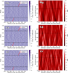 |
Fig. G.2 NIRPS non-detections, G.1 continued. |
| In the text | |
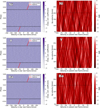 |
Fig. G.3 NIRPS non-detections, G.1 continued. |
| In the text | |
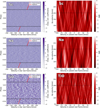 |
Fig. G.4 NIRPS non-detections, G.1 continued. |
| In the text | |
|
Fig. G.5 NIRPS non-detections, G.1 continued. Remnants of the telluric correction (beyond and within in-transit phases) are visible in the water and OH cross-correlation maps. |
| In the text | |
|
Fig. H.1 HARPS cross-correlation results showing non-detected chemical species. |
| In the text | |
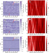 |
Fig. H.2 HARPS non-detections, H.1 continued. |
| In the text | |
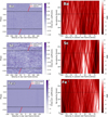 |
Fig. H.3 HARPS non-detections, H.1 continued. |
| In the text | |
|
Fig. H.4 HARPS non-detections, H.1 continued. The cross-correlation maps for H2O present features around 25 km s−1 due to remnant artefacts of the telluric correction. |
| In the text | |
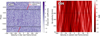 |
Fig. H.5 HARPS non-detections, H.1 continued. |
| In the text | |
|
Fig. I.1 Cross-correlation detection of Fe from the HARPS transits, but now using a blind data-driven PCA-based detrending algorithm instead. The white dashed lines denote the expected Kp and vsys (Kp=200.7 km s−1 and vsys=−24.45 km s−1; Prinoth et al. 2022; Anderson et al. 2018) of WASP-189b assuming a uniform and static atmosphere. The white blob near the expected location shows the observed signal of WASP-189b. Differently from Figure 6, 7, 8, and, H.1, G.1, this map has been generated from transmission spectra non-shifted by the systemic velocity. The uniformness of the CCF map between 0 and 50 km s−1 at low Kp values is a result of the Rossiter-McLaughlin mask excluding values overlapping with the Doppler shadow in radial velocity space. The data product that produced this CCF map is the input for the atmospheric retrieval analysis (Section 5.3). |
| In the text | |
Current usage metrics show cumulative count of Article Views (full-text article views including HTML views, PDF and ePub downloads, according to the available data) and Abstracts Views on Vision4Press platform.
Data correspond to usage on the plateform after 2015. The current usage metrics is available 48-96 hours after online publication and is updated daily on week days.
Initial download of the metrics may take a while.