| Issue |
A&A
Volume 697, May 2025
|
|
|---|---|---|
| Article Number | A85 | |
| Number of page(s) | 22 | |
| Section | Cosmology (including clusters of galaxies) | |
| DOI | https://doi.org/10.1051/0004-6361/202452480 | |
| Published online | 12 May 2025 | |
Euclid preparation
LXIX. The impact of relativistic redshift-space distortions on two-point clustering statistics from the Euclid wide spectroscopic survey
1
INFN-Padova, Via Marzolo 8, 35131 Padova, Italy
2
Dipartimento di Fisica e Astronomia “G. Galilei”, Università di Padova, Via Marzolo 8, 35131 Padova, Italy
3
INAF-Osservatorio Astronomico di Padova, Via dell’Osservatorio 5, 35122 Padova, Italy
4
Universität Bonn, Argelander-Institut für Astronomie, Auf dem Hügel 71, 53121 Bonn, Germany
5
Dipartimento di Fisica – Sezione di Astronomia, Università di Trieste, Via Tiepolo 11, 34131 Trieste, Italy
6
INAF-Osservatorio Astronomico di Trieste, Via G. B. Tiepolo 11, 34143 Trieste, Italy
7
IFPU, Institute for Fundamental Physics of the Universe, Via Beirut 2, 34151 Trieste, Italy
8
INFN, Sezione di Trieste, Via Valerio 2, 34127 Trieste, TS, Italy
9
Université Paris-Saclay, CNRS, Institut d’astrophysique spatiale, 91405 Orsay, France
10
School of Mathematics and Physics, University of Surrey, Guildford, Surrey GU2 7XH, UK
11
INAF-Osservatorio Astronomico di Brera, Via Brera 28, 20122 Milano, Italy
12
INAF-Osservatorio di Astrofisica e Scienza dello Spazio di Bologna, Via Piero Gobetti 93/3, 40129 Bologna, Italy
13
SISSA, International School for Advanced Studies, Via Bonomea 265, 34136 Trieste, TS, Italy
14
Dipartimento di Fisica e Astronomia, Università di Bologna, Via Gobetti 93/2, 40129 Bologna, Italy
15
INFN-Sezione di Bologna, Viale Berti Pichat 6/2, 40127 Bologna, Italy
16
Max Planck Institute for Extraterrestrial Physics, Giessenbachstr. 1, 85748 Garching, Germany
17
INAF-Osservatorio Astrofisico di Torino, Via Osservatorio 20, 10025 Pino Torinese (TO), Italy
18
Dipartimento di Fisica, Università di Genova, Via Dodecaneso 33, 16146 Genova, Italy
19
INFN-Sezione di Genova, Via Dodecaneso 33, 16146 Genova, Italy
20
Department of Physics “E. Pancini”, University Federico II, Via Cinthia 6, 80126 Napoli, Italy
21
INAF-Osservatorio Astronomico di Capodimonte, Via Moiariello 16, 80131 Napoli, Italy
22
INFN section of Naples, Via Cinthia 6, 80126 Napoli, Italy
23
Instituto de Astrofísica e Ciências do Espaço, Universidade do Porto, CAUP, Rua das Estrelas, PT4150-762 Porto, Portugal
24
Dipartimento di Fisica, Università degli Studi di Torino, Via P. Giuria 1, 10125 Torino, Italy
25
INFN-Sezione di Torino, Via P. Giuria 1, 10125 Torino, Italy
26
INAF-IASF Milano, Via Alfonso Corti 12, 20133 Milano, Italy
27
INAF-Osservatorio Astronomico di Roma, Via Frascati 33, 00078 Monteporzio Catone, Italy
28
INFN-Sezione di Roma, Piazzale Aldo Moro, 2 – c/o Dipartimento di Fisica, Edificio G. Marconi, 00185 Roma, Italy
29
Centro de Investigaciones Energéticas, Medioambientales y Tecnológicas (CIEMAT), Avenida Complutense 40, 28040 Madrid, Spain
30
Port d’Informació Científica, Campus UAB, C. Albareda s/n, 08193 Bellaterra (Barcelona), Spain
31
Institut d’Estudis Espacials de Catalunya (IEEC), Edifici RDIT, Campus UPC, 08860 Castelldefels, Barcelona, Spain
32
Institute of Space Sciences (ICE, CSIC), Campus UAB, Carrer de Can Magrans, s/n, 08193 Barcelona, Spain
33
Institute for Theoretical Particle Physics and Cosmology (TTK), RWTH Aachen University, 52056 Aachen, Germany
34
Dipartimento di Fisica e Astronomia “Augusto Righi” – Alma Mater Studiorum Università di Bologna, Viale Berti Pichat 6/2, 40127 Bologna, Italy
35
Instituto de Astrofísica de Canarias, Calle Vía Láctea s/n, 38204 San Cristóbal de La Laguna, Tenerife, Spain
36
Institute for Astronomy, University of Edinburgh, Royal Observatory, Blackford Hill, Edinburgh EH9 3HJ, UK
37
Jodrell Bank Centre for Astrophysics, Department of Physics and Astronomy, University of Manchester, Oxford Road, Manchester M13 9PL, UK
38
European Space Agency/ESRIN, Largo Galileo Galilei 1, 00044 Frascati, Roma, Italy
39
ESAC/ESA, Camino Bajo del Castillo, s/n., Urb. Villafranca del Castillo, 28692 Villanueva de la Cañada, Madrid, Spain
40
Université Claude Bernard Lyon 1, CNRS/IN2P3, IP2I Lyon, UMR 5822, Villeurbanne F-69100, France
41
Institute of Physics, Laboratory of Astrophysics, Ecole Polytechnique Fédérale de Lausanne (EPFL), Observatoire de Sauverny, 1290 Versoix, Switzerland
42
UCB Lyon 1, CNRS/IN2P3, IUF, IP2I Lyon, 4 rue Enrico Fermi, 69622 Villeurbanne, France
43
Departamento de Física, Faculdade de Ciências, Universidade de Lisboa, Edifício C8, Campo Grande, PT1749-016 Lisboa, Portugal
44
Instituto de Astrofísica e Ciências do Espaço, Faculdade de Ciências, Universidade de Lisboa, Campo Grande, 1749-016 Lisboa, Portugal
45
Department of Astronomy, University of Geneva, ch. d’Ecogia 16, 1290 Versoix, Switzerland
46
INAF-Istituto di Astrofisica e Planetologia Spaziali, Via del Fosso del Cavaliere, 100, 00100 Roma, Italy
47
Université Paris-Saclay, Université Paris Cité, CEA, CNRS, AIM, 91191 Gif-sur-Yvette, France
48
Institut de Ciencies de l’Espai (IEEC-CSIC), Campus UAB, Carrer de Can Magrans, s/n Cerdanyola del Vallés, 08193 Barcelona, Spain
49
Istituto Nazionale di Fisica Nucleare, Sezione di Bologna, Via Irnerio 46, 40126 Bologna, Italy
50
FRACTAL S.L.N.E., calle Tulipán 2, Portal 13 1A, 28231 Las Rozas de Madrid, Spain
51
Universitäts-Sternwarte München, Fakultät für Physik, Ludwig-Maximilians-Universität München, Scheinerstrasse 1, 81679 München, Germany
52
Dipartimento di Fisica “Aldo Pontremoli”, Università degli Studi di Milano, Via Celoria 16, 20133 Milano, Italy
53
Institute of Theoretical Astrophysics, University of Oslo, PO Box 1029 Blindern 0315 Oslo, Norway
54
Jet Propulsion Laboratory, California Institute of Technology, 4800 Oak Grove Drive, Pasadena, CA 91109, USA
55
Felix Hormuth Engineering, Goethestr. 17, 69181 Leimen, Germany
56
Technical University of Denmark, Elektrovej 327, 2800 Kgs. Lyngby, Denmark
57
Cosmic Dawn Center (DAWN), Copenhagen N, Denmark
58
Max-Planck-Institut für Astronomie, Königstuhl 17, 69117 Heidelberg, Germany
59
NASA Goddard Space Flight Center, Greenbelt, MD 20771, USA
60
Department of Physics and Astronomy, University College London, Gower Street, London WC1E 6BT, UK
61
Department of Physics and Helsinki Institute of Physics, Gustaf Hällströmin katu 2, 00014 University of Helsinki, Finland
62
Aix-Marseille Université, CNRS/IN2P3, CPPM, Marseille, France
63
Mullard Space Science Laboratory, University College London, Holmbury St Mary, Dorking, Surrey RH5 6NT, UK
64
Leiden Observatory, Leiden University, Einsteinweg 55, 2333 CC Leiden, The Netherlands
65
Université de Genève, Département de Physique Théorique and Centre for Astroparticle Physics, 24 quai Ernest-Ansermet, CH-1211 Genève 4, Switzerland
66
Department of Physics, PO Box 64 00014 University of Helsinki, Finland
67
Helsinki Institute of Physics, Gustaf Hällströmin katu 2, University of Helsinki, Helsinki, Finland
68
NOVA optical infrared instrumentation group at ASTRON, Oude Hoogeveensedijk 4, 7991 PD Dwingeloo, The Netherlands
69
Centre de Calcul de l’IN2P3/CNRS, 21 avenue Pierre de Coubertin, 69627 Villeurbanne Cedex, France
70
Aix-Marseille Université, CNRS, CNES, LAM, Marseille, France
71
Dipartimento di Fisica e Astronomia “Augusto Righi” – Alma Mater Studiorum Università di Bologna, Via Piero Gobetti 93/2, 40129 Bologna, Italy
72
Department of Physics, Institute for Computational Cosmology, Durham University, South Road, DH1 3LE Durham, UK
73
Université Paris Cité, CNRS, Astroparticule et Cosmologie, 75013 Paris, France
74
Institut d’Astrophysique de Paris, 98bis Boulevard Arago, 75014 Paris, France
75
Institut d’Astrophysique de Paris, UMR 7095, CNRS, and Sorbonne Université, 98 bis boulevard Arago, 75014 Paris, France
76
European Space Agency/ESTEC, Keplerlaan 1, 2201 AZ Noordwijk, The Netherlands
77
Institut de Física d’Altes Energies (IFAE), The Barcelona Institute of Science and Technology, Campus UAB, 08193 Bellaterra, (Barcelona), Spain
78
Department of Physics and Astronomy, University of Aarhus, Ny Munkegade 120, DK-8000 Aarhus C, Denmark
79
Space Science Data Center, Italian Space Agency, Via del Politecnico snc, 00133 Roma, Italy
80
Centre National d’Etudes Spatiales – Centre spatial de Toulouse, 18 avenue Edouard Belin, 31401 Toulouse Cedex 9, France
81
Institute of Space Science, Str. Atomistilor, nr. 409 Măgurele, Ilfov 077125, Romania
82
Departamento de Astrofísica, Universidad de La Laguna, 38206 La Laguna, Tenerife, Spain
83
Institut für Theoretische Physik, University of Heidelberg, Philosophenweg 16, 69120 Heidelberg, Germany
84
Institut de Recherche en Astrophysique et Planétologie (IRAP), Université de Toulouse, CNRS, UPS, CNES, 14 Av. Edouard Belin, 31400 Toulouse, France
85
Université St Joseph; Faculty of Sciences, Beirut, Lebanon
86
Departamento de Física, FCFM, Universidad de Chile, Blanco Encalada 2008, Santiago, Chile
87
Universität Innsbruck, Institut für Astro- und Teilchenphysik, Technikerstr. 25/8, 6020 Innsbruck, Austria
88
Satlantis, University Science Park, Sede Bld 48940, Leioa-Bilbao, Spain
89
Instituto de Astrofísica e Ciências do Espaço, Faculdade de Ciências, Universidade de Lisboa, Tapada da Ajuda, 1349-018 Lisboa, Portugal
90
Universidad Politécnica de Cartagena, Departamento de Electrónica y Tecnología de Computadoras, Plaza del Hospital 1, 30202 Cartagena, Spain
91
INFN-Bologna, Via Irnerio 46, 40126 Bologna, Italy
92
Kapteyn Astronomical Institute, University of Groningen, PO Box 800 9700 AV Groningen, The Netherlands
93
Dipartimento di Fisica, Università degli studi di Genova, and INFN-Sezione di Genova, Via Dodecaneso 33, 16146 Genova, Italy
94
Infrared Processing and Analysis Center, California Institute of Technology, Pasadena, CA 91125, USA
95
INAF, Istituto di Radioastronomia, Via Piero Gobetti 101, 40129 Bologna, Italy
96
Astronomical Observatory of the Autonomous Region of the Aosta Valley (OAVdA), Loc. Lignan 39, I-11020 Nus (Aosta Valley), Italy
97
Junia, EPA department, 41 Bd Vauban, 59800 Lille, France
98
ICSC – Centro Nazionale di Ricerca in High Performance Computing, Big Data e Quantum Computing, Via Magnanelli 2, Bologna, Italy
99
Instituto de Física Teórica UAM-CSIC, Campus de Cantoblanco, 28049 Madrid, Spain
100
CERCA/ISO, Department of Physics, Case Western Reserve University, 10900 Euclid Avenue, Cleveland, OH 44106, USA
101
Laboratoire Univers et Théorie, Observatoire de Paris, Université PSL, Université Paris Cité, CNRS, 92190 Meudon, France
102
Dipartimento di Fisica e Scienze della Terra, Università degli Studi di Ferrara, Via Giuseppe Saragat 1, 44122 Ferrara, Italy
103
Istituto Nazionale di Fisica Nucleare, Sezione di Ferrara, Via Giuseppe Saragat 1, 44122 Ferrara, Italy
104
Kavli Institute for the Physics and Mathematics of the Universe (WPI), University of Tokyo, Kashiwa, Chiba 277-8583, Japan
105
Ludwig-Maximilians-University, Schellingstrasse 4, 80799 Munich, Germany
106
Max-Planck-Institut für Physik, Boltzmannstr. 8, 85748 Garching, Germany
107
Minnesota Institute for Astrophysics, University of Minnesota, 116 Church St SE, Minneapolis, MN 55455, USA
108
Institute Lorentz, Leiden University, Niels Bohrweg 2, 2333 CA Leiden, The Netherlands
109
Université Côte d’Azur, Observatoire de la Côte d’Azur, CNRS, Laboratoire Lagrange, Bd de l’Observatoire, CS 34229, 06304 Nice cedex 4, France
110
Institute for Astronomy, University of Hawaii, 2680 Woodlawn Drive, Honolulu, HI 96822, USA
111
Department of Physics & Astronomy, University of California Irvine, Irvine, CA 92697, USA
112
Department of Astronomy & Physics and Institute for Computational Astrophysics, Saint Mary’s University, 923 Robie Street, Halifax, Nova Scotia B3H 3C3, Canada
113
Departamento Física Aplicada, Universidad Politécnica de Cartagena, Campus Muralla del Mar, 30202 Cartagena, Murcia, Spain
114
Instituto de Astrofísica de Canarias (IAC); Departamento de Astrofísica, Universidad de La Laguna (ULL), 38200 La Laguna, Tenerife, Spain
115
Department of Physics, Oxford University, Keble Road, Oxford OX1 3RH, UK
116
Institute of Cosmology and Gravitation, University of Portsmouth, Portsmouth PO1 3FX, UK
117
Department of Computer Science, Aalto University, PO Box 15400, Espoo FI-00 076, Finland
118
Ruhr University Bochum, Faculty of Physics and Astronomy, Astronomical Institute (AIRUB), German Centre for Cosmological Lensing (GCCL), 44780 Bochum, Germany
119
DARK, Niels Bohr Institute, University of Copenhagen, Jagtvej 155, 2200 Copenhagen, Denmark
120
Univ. Grenoble Alpes, CNRS, Grenoble INP, LPSC-IN2P3, 53, Avenue des Martyrs, 38000 Grenoble, France
121
Department of Physics and Astronomy, Vesilinnantie 5, 20014 University of Turku, Finland
122
Serco for European Space Agency (ESA), Camino bajo del Castillo, s/n, Urbanizacion Villafranca del Castillo, Villanueva de la Cañada, 28692 Madrid, Spain
123
ARC Centre of Excellence for Dark Matter Particle Physics, Melbourne, Australia
124
Centre for Astrophysics & Supercomputing, Swinburne University of Technology, Hawthorn, Victoria 3122, Australia
125
School of Physics and Astronomy, Queen Mary University of London, Mile End Road, London E1 4NS, UK
126
Department of Physics and Astronomy, University of the Western Cape, Bellville, Cape Town 7535, South Africa
127
Université Libre de Bruxelles (ULB), Service de Physique Théorique CP225, Boulevard du Triophe, 1050 Bruxelles, Belgium
128
ICTP South American Institute for Fundamental Research, Instituto de Física Teórica, Universidade Estadual Paulista, São Paulo, Brazil
129
Oskar Klein Centre for Cosmoparticle Physics, Department of Physics, Stockholm University, Stockholm SE-106 91, Sweden
130
Astrophysics Group, Blackett Laboratory, Imperial College London, London SW7 2AZ, UK
131
INAF-Osservatorio Astrofisico di Arcetri, Largo E. Fermi 5, 50125 Firenze, Italy
132
Dipartimento di Fisica, Sapienza Università di Roma, Piazzale Aldo Moro 2, 00185 Roma, Italy
133
Centro de Astrofísica da Universidade do Porto, Rua das Estrelas, 4150-762 Porto, Portugal
134
Dipartimento di Fisica, Università di Roma Tor Vergata, Via della Ricerca Scientifica 1, Roma, Italy
135
INFN, Sezione di Roma 2, Via della Ricerca Scientifica 1, Roma, Italy
136
Institute of Astronomy, University of Cambridge, Madingley Road, Cambridge CB3 0HA, UK
137
Department of Astrophysics, University of Zurich, Winterthurerstrasse 190, 8057 Zurich, Switzerland
138
Theoretical astrophysics, Department of Physics and Astronomy, Uppsala University, Box 515 751 20 Uppsala, Sweden
139
Department of Physics, Royal Holloway, University of London, Surrey TW20 0EX, UK
140
Department of Astrophysical Sciences, Peyton Hall, Princeton University, Princeton, NJ 08544, USA
141
Niels Bohr Institute, University of Copenhagen, Jagtvej 128, 2200 Copenhagen, Denmark
142
Institut de Physique Théorique, CEA, CNRS, Université Paris-Saclay, 91191 Gif-sur-Yvette Cedex, France
143
Center for Cosmology and Particle Physics, Department of Physics, New York University, New York, NY 10003, USA
144
Center for Computational Astrophysics, Flatiron Institute, 162 5th Avenue, 10010 New York, NY, USA
⋆ Corresponding author: mohamed.elkhashab@inaf.it
Received:
4
October
2024
Accepted:
28
February
2025
Measurements of galaxy clustering are affected by redshift-space distortions (RSDs). Peculiar velocities, gravitational lensing, and other light-cone projection effects modify the observed redshifts, fluxes, and sky positions of distant light sources. We determined which of these effects leave a detectable imprint on several two-point clustering statistics to be extracted from the Euclid wide spectroscopic survey (EWSS) on large scales. We generated 140 mock galaxy catalogues with the survey geometry and selection function of the EWSS and made use of the LIGER (LIght cones with GEneral Relativity) method to account for a variable number of relativistic RSDs to linear order in the cosmological perturbations. We estimated different two-point clustering statistics from the mocks and used the likelihood-ratio test to calculate the statistical significance with which the EWSS could reject the null hypothesis that certain relativistic projection effects can be neglected in the theoretical models. We find that the combined effects of lensing magnification and convergence imprint characteristic signatures on several clustering observables. Their signal-to-noise ratio (S/N) ranges between 2.5 and 6 (depending on the adopted summary statistic) for the highest-redshift galaxies in the EWSS. The corresponding feature due to the peculiar velocity of the Sun is measured with a S/N of order one or two. The multipoles of the power spectrum from the catalogues that include all relativistic effects reject the null hypothesis that RSDs are only generated by the variation in the peculiar velocity along the line of sight with a significance of 2.9 standard deviations. As a by-product of our study, we demonstrate that the mixing-matrix formalism to model finite-volume effects in the multipole moments of the power spectrum can be robustly applied to surveys made of several disconnected patches. Our results indicate that relativistic RSDs, in particular the contribution from weak gravitational lensing, cannot be disregarded when modelling two-point clustering statistics extracted from the EWSS.
Key words: methods: numerical / galaxies: statistics / large-scale structure of Universe
© The Authors 2025
 Open Access article, published by EDP Sciences, under the terms of the Creative Commons Attribution License (https://creativecommons.org/licenses/by/4.0), which permits unrestricted use, distribution, and reproduction in any medium, provided the original work is properly cited.
This article is published in open access under the Subscribe to Open model. Subscribe to A&A to support open access publication.
1. Introduction
The primary science goal of the recently launched Euclid space mission (Euclid Collaboration: Mellier et al. 2025) is to test whether a cosmological constant can be ruled out as the driver of the accelerated expansion of the Universe. To that end, Euclid is carrying out a wide-angle survey covering nearly 15 000 deg2 of the extragalactic sky. The Euclid mission is optimised for the combination of two cosmological probes – weak gravitational lensing and galaxy clustering – and relies on two instruments. The visual imager (VIS, Euclid Collaboration: Borlaff et al. 2022) operates in the 550 to 900 nm pass-band and produces high-quality galaxy images to perform measurements of galaxy shapes (cosmic shear). The near-infrared spectrometer and photometer (NISP, Maciaszek et al. 2022; Euclid Collaboration: Schirmer et al. 2022) carries out imaging photometry (as an input for the estimation of photometric redshifts) and slitless spectroscopy to precisely measure the redshift of the Hα emission line in the range 0.9 < z < 1.8. Over six years of observations, the Euclid wide spectroscopic survey (EWSS) will measure the redshifts and positions of nearly 30 million emission-line galaxies, while its photometric counterpart will measure the positions and shapes of approximately 1.5 billion galaxies.
Galaxy clustering (the only cosmological probe discussed in this paper) sets constraints on the cause of the accelerated expansion of the Universe in two ways. First, the expansion history of the Universe can be reconstructed by locating the characteristic scale imprinted by baryonic acoustic oscillations on the galaxy power spectrum (or the two-point correlation function, 2PCF) as a function of redshift (e.g. Cole et al. 2005; Eisenstein et al. 2005). Second, the growth rate of structure can be determined by studying the anisotropy of the clustering signal (e.g. Peacock et al. 2001). The latter option is generally known as the study of redshift-space distortions (RSDs), which arise when galaxy redshifts are mapped into distances by assuming an unperturbed Friedmann-Lemaître-Robertson-Walker (FLRW) metric. The observed redshift of a galaxy does not coincide with its cosmological component. The dominant (but not sole) correction is due to the relative peculiar velocity between the galaxy and the observer along the line of sight. In a seminal work, Kaiser (1987) used linear perturbation theory to calculate how peculiar velocities distort the galaxy power spectrum (in the Cartesian Fourier basis, see also Hamilton & Culhane 1996; Hamilton 1998, 2000, for extensions to configuration space). The derivation relies on a simplifying assumption that the size of the surveyed region is negligibly small compared to its distance from the observer, so that the lines of sight to all galaxies are effectively parallel. This is nowadays known as the ‘global plane-parallel’ (GPP) approximation and implies that the galaxy power spectrum depends on the cosine of the angle between the wavevector and the fixed line of sight. When decomposed in Legendre polynomials, this functional dependence only includes multipoles of degree 0, 2, and 4.
The EWSS provides us with the opportunity to study galaxy clustering on unprecedentedly large scales. This possibility, however, brings forth new challenges. First of all, galaxy pairs with large angular separations contribute to the clustering signal and might cause systematic deviations of the observations from models based on the GPP approximation. Wide-angle effects have been investigated both for the galaxy 2PCF (see e.g. Matsubara 2000a; Szapudi 2004; Pápai & Szapudi 2008; Raccanelli et al. 2010; Samushia et al. 2012; Raccanelli et al. 2018) and the power spectrum (see e.g. Zaroubi & Hoffman 1996; Reimberg et al. 2016; Castorina & White 2018; Castorina et al. 2019). The current leading opinion is that accounting for a variable line-of-sight using the ‘local plane-parallel’ (LPP) approach (e.g. Beutler et al. 2014; Wilson et al. 2017) is sufficient for conducting cosmological studies with surveys of similar size and depth to the EWSS (Castorina & Di Dio 2022; Noorikuhani & Scoccimarro 2023). An alternative approach that fully accounts for wide-angle effects is to forgo the plane-wave expansion of the Fourier-space overdensity and instead adopt the ‘spherical Fourier-Bessel’ formalism (e.g. Heavens & Taylor 1995; Hamilton 2005; Yoo & Desjacques 2013). The second complication arises from the fact that Kaiser’s RSDs should be complemented with additional corrections. The light bundles from distant galaxies to us propagate through the inhomogeneous Universe and are thus subject to effects like gravitational lensing or aberration. Hence, the observed galaxy positions on the sky, redshifts, and fluxes differ from their analogues obtained in the corresponding unperturbed FLRW model. However, we construct maps of the galaxy distribution by assuming such a homogeneous model in order to convert the observed properties into three-dimensional positions and luminosities. This step introduces a number of artefacts in the galaxy overdensity field (Yoo et al. 2009; Bonvin & Durrer 2011; Challinor & Lewis 2011; Jeong et al. 2012) that we refer to as ‘relativistic1 RSDs’ and that are also known in the literature as ‘relativistic effects’ or ‘projection effects’ (since we observe the projection of the actual Universe on our past light cone). These alterations can be studied perturbatively. The leading term coincides with Kaiser’s RSDs due to the peculiar velocity gradient along the line of sight. Nevertheless, there exist several additional corrections that can potentially influence galaxy-clustering statistics on very large scales. A number of investigations have characterised the impact of these terms on the angular power spectrum (Di Dio et al. 2013; Borzyszkowski et al. 2017), the 2PCF (e.g. Bertacca 2015; Raccanelli et al. 2016; Tansella et al. 2018; Bertacca 2020; Jelic-Cizmek et al. 2021; Breton et al. 2022, 2019), and the (3D) power spectrum (Elkhashab et al. 2021; Castorina & Di Dio 2022; Foglieni et al. 2023; Noorikuhani & Scoccimarro 2023).
Finding out which of the relativistic RSDs will leave a detectable imprint on the two-point summary statistics measured from the EWSS is the main goal of this study2. We investigated four different suites of mock galaxy catalogues built with the LIGER (LIght cones with GEneral Relativity) method (Borzyszkowski et al. 2017; Elkhashab et al. 2021), which allows us to self-consistently correct the output of Newtonian N-body simulations and introduce relativistic RSDs to linear order in the cosmological perturbations. All the mock catalogues we generated match the survey geometry and selection function of the EWSS but the four kinds we consider differ in the number of RSD terms they include. This helped us to isolate the contributions from various effects (e.g. gravitational lensing or the peculiar velocity of the observer). We made use of popular estimators to measure clustering summary statistics from the mock catalogues and we built unbiased models that exactly account for wide-angle effects by averaging the measurements over a large number of realisations. For the power spectrum and 2PCF multipoles, we adopted the standard statistics (and estimators) that will be used for the cosmological analysis for the EWSS. Finally, we employed the likelihood-ratio test to quantify the signal-to-noise ratio (S/N) with which certain effects can be detected and to determine the fraction of realisations in which models that do not account for these effects could be ruled out with a given statistical significance.
The paper is structured as follows. We introduce the relativistic RSDs in Sect. 2 and our mock EWSS galaxy catalogues in Sect. 3. We describe how we assess the detectability of various relativistic RSDs in Sect. 4. Our results for the angular power spectrum, the multipole moments of the 2PCF, and the multipole moments of the power spectrum are presented in Sects. 5, 6, and 7, respectively. Moreover, in Sect. 8, we compare the power-spectrum multipoles extracted from the mocks to the predictions from Kaiser’s model after accounting for the window function of the survey and the integral constraint. Eventually, in Sect. 9, we summarise our findings and conclude.
Throughout this paper, we adopt Einstein’s summation convention and define the space-time metric tensor to have the signature ( − , + , + , + ). Greek indices refer to space-time components (i.e. run from 0 to 3), while Latin indices label spatial components (i.e. run from 1 to 3). Furthermore, the Dirac delta and the Kronecker delta functions are denoted by the symbols δD and δK, respectively. Our Fourier-transform convention is  . Finally, the symbol c denotes the speed of light in vacuum.
2. Relativistic RSDs
In order to build three-dimensional maps of the galaxy distribution, it is usually assumed that the light bundles emitted by the galaxies propagate in an unperturbed FLRW model universe and that their observed redshift, zobs, coincides with the cosmological one. This implies that their comoving distance in the so-called ‘redshift space’ is
where H(z) denotes the Hubble parameter in the model universe as a function of redshift. This procedure, however, neglects the fact that inhomogeneities in the Universe alter the observed redshifts and angular positions of the galaxies. Therefore, the reconstructed galaxy maps in redshift space are not faithful (Sargent & Turner 1977). A number of effects, collectively called redshift-space distortions, artificially shift the reconstructed positions of galaxies in both the radial and tangential directions with respect to their actual (hereafter, real-space) location.
The pioneering work by Kaiser (1987) investigated the relationship between galaxy densities in real and redshift space at linear order in the cosmological perturbations, focusing on the impact of peculiar velocities generated by gravitational instabilities (see also Hamilton & Culhane 1996; Hamilton 1998; Matsubara 2000b). More recently, this subject has been revisited using a fully general-relativistic approach and accounting for additional effects like gravitational lensing, the Sachs–Wolfe effects, and the Shapiro delay (Yoo et al. 2009; Bonvin & Durrer 2011; Challinor & Lewis 2011; Jeong et al. 2012). In this latter case, the goal is to compute the geodesics of photons emitted from a source galaxy in the presence of linear cosmological perturbations. This is sufficient to address the large spatial scales considered in this paper. In the remainder of this section we summarise the main results obtained within the general-relativistic framework.
By definition, the co-ordinates of a distant galaxy in redshift space can be trivially expressed as
where η0 is the present-day value of conformal time (i.e. at observation), x denotes the comoving distance from the observer (see Eq. 1), and n is the observed galaxy position (pointing towards the galaxy) on the sky. The mapping between the real- and redshift-space co-ordinates of a galaxy can be generically written as xrμ = xμ + Δxμ. In order to compute the co-ordinate transformation explicitly, we need to specify a gauge. We express the space-time metric in the Poisson gauge, assuming a flat cosmology while neglecting vector and tensor perturbations3,
![$$ \begin{aligned} {\mathrm{d} } s^2 = a^2(\eta )\left[-(1+2\Psi )\,c^2\,{\mathrm{d} }\eta ^2 +(1-2{\Phi })\,\delta _{\mathrm{K}\,ij}\, {\mathrm{d} } x^i\;{\mathrm{d} } x^j\;\right]\,, \end{aligned} $$](/articles/aa/full_html/2025/05/aa52480-24/aa52480-24-eq4.gif)
where Ψ and Φ are the dimensionless Bardeen potentials, η is the conformal time, and a is the cosmic scale factor. From this choice, it follows that (Hui & Greene 2006; Yoo et al. 2009; Bonvin & Durrer 2011; Challinor & Lewis 2011; Jeong et al. 2012)
where
![$$ \begin{aligned} \delta \ln a := \left[{(\boldsymbol{v}_{\rm e}-\boldsymbol{v}_{\rm o})\over c }\cdot \boldsymbol{{n}} - (\Phi _{\rm e}-\Phi _{\rm o}) - \int _0^x {(\Phi \prime + \Psi \prime )\over c}\;{\mathrm{d} } \tilde{x}\right]\,, \end{aligned} $$](/articles/aa/full_html/2025/05/aa52480-24/aa52480-24-eq7.gif)
represents the fractional redshift change due to the perturbations; that is, −δz/(1 + z). Here, v denotes peculiar three-velocities, the subscripts ‘e’ and ‘o’ specify whether the functions are evaluated at the source or observer locations, respectively,  , ℋ = a(zobs) H(zobs), and the prime superscript denotes the partial derivative w.r.t. η. It is worth mentioning that the equations above assume that the peculiar velocity of a galaxy coincides with that of the matter at the same location; in other words, that there is no velocity bias4.
Cosmological perturbations also alter the solid angle under which galaxies are seen by distant observers, thus enhancing, or decreasing their apparent flux (e.g. Broadhurst et al. 1995). In terms of the luminosity distance, DL, the magnification of a galaxy is defined as
where  denotes the luminosity distance in the background model universe evaluated at zobs. At linear order (e.g. Challinor & Lewis 2011; Bertacca 2015),
where the weak lensing convergence is
![$$ \begin{aligned} \kappa := {1\over 2}\int ^x_0\, (x-\tilde{x})\,\frac{\tilde{x}}{x} \left[\nabla ^2 +(\boldsymbol{n}\cdot \boldsymbol{\nabla })^2 - {2\over x} \boldsymbol{n}\cdot \boldsymbol{\nabla } \right] (\Phi + \Psi )\; {\mathrm{d} } \tilde{x}\,. \end{aligned} $$](/articles/aa/full_html/2025/05/aa52480-24/aa52480-24-eq12.gif)
The next step is to understand how the local number density of galaxies in a survey responds to redshift perturbations and magnification. To first approximation, the EWSS is flux limited as it only selects galaxies above a given observed Hα flux5, corresponding to a redshift-dependent luminosity limit, Llim(z). We indicate by n(Lmin, z) the mean number density of the target population of galaxies with luminosity L > Lmin at redshift z. Then, the so-called evolution bias,
quantifies how rapidly the number density of the selected galaxies changes with redshift. Similarly, the magnification bias,
gives the slope of the cumulative luminosity function evaluated at the luminosity limit of the survey. Taking into account all linear-order corrections to the ‘observed’ galaxy density (in redshift space), ng, and its angular average at fixed zobs,  , it is possible to express the overdensity,
  , in terms of the cosmological perturbations (Yoo et al. 2009; Challinor & Lewis 2011; Jeong et al. 2012; Bertacca 2015)
![$$ \begin{aligned} \delta _{\rm g, s}(\boldsymbol{x})&= \delta ^\mathrm{com}_{\rm g}-\frac{1}{{\mathcal{H} }}\frac{\partial (\boldsymbol{v}_{\rm e}\cdot \boldsymbol{n})}{\partial x}+ 2\,(\mathcal{Q} -1) \,{\kappa }\nonumber \\ \nonumber&\quad + \left[ \mathcal{E} -2\mathcal{Q} - \frac{{\mathcal{H} }\prime }{{\mathcal{H} }^2} - \frac{2(1-\mathcal{Q} )\,c}{x\, {\mathcal{H} }}\right]\\&\quad \times \left[{\boldsymbol{v}_{\rm e}\over c}\cdot \boldsymbol{n} - (\Phi _{\rm e}-\Phi _{\rm o}) - \int _0^x {(\Phi \prime + \Psi \prime )\over c}\;{\mathrm{d} } \tilde{x}\right]\nonumber \\\nonumber&\quad -2\,(1-\mathcal{Q} )\,\Phi _{\rm e}+\Psi _{\rm e} + {\Phi _{\rm e}\prime \over \mathcal{H} } + \left(3- \mathcal{E} \right)\frac{\mathcal{H} \Theta }{{c}^2} \nonumber \\&\quad +\frac{2\,(1-\mathcal{Q} )}{x} \int _0^x(\Phi +\Psi )\;{\mathrm{d} } \tilde{x}\,\nonumber \\&\quad +\left[2- \mathcal{E} + \frac{{\mathcal{H} }\prime }{{\mathcal{H} }^2} + \frac{2\,(1-\mathcal{Q} )\,c}{x\, {\mathcal{H} }}\right]{\boldsymbol{v}_{\rm o}\over c}\cdot \boldsymbol{n}\;, \end{aligned} $$](/articles/aa/full_html/2025/05/aa52480-24/aa52480-24-eq17.gif)
where Θ is the linear velocity potential (i.e. v = ∇ Θ). We note that the real-space galaxy overdensity,  , is defined in the synchronous comoving gauge while all the rest is set in the Poisson gauge6. At linear order,
  is related to the underlying matter density fluctuation through the linear bias parameter b; that is,
  (Challinor & Lewis 2011; Jeong et al. 2012).
Equation (11) defines what is meant by ‘relativistic (linear) RSDs’ and forms the starting point for our study. In brief, it says that the galaxy overdensities in real and redshift space differ because of a number of physical effects. The second term on the rhs is the classic Kaiser correction due to the variation in peculiar velocities along the line of sight (Kaiser 1987). The third term is the weak lensing contribution due to volume and magnification corrections, which is expected to have an effect on different clustering statistics on large scales (e.g. Matsubara 2000b; Hui et al. 2007, 2008; Yoo et al. 2009; Challinor & Lewis 2011; Camera et al. 2015; Raccanelli et al. 2016; Borzyszkowski et al. 2017). There are then several additional corrections that depend on the gravitational potentials and the peculiar velocities. Previous studies have shown that those proportional to the peculiar velocity of the observer – that is, the last term in Eq. (11) – could generate observable features in the 2PCF at wide angles (Bertacca 2020) as well as superimpose an oscillatory signal to the power-spectrum monopole at very large scales (Elkhashab et al. 2021, see also Bahr-Kalus et al. 2021), dubbed the finger-of-the-observer effect.
3. Galaxy mocks
In this paper, we use a suite of realistic mock galaxy catalogues to determine which of the corrections appearing in Eq. (11) should be accounted for in the analysis of two-point clustering statistics extracted from the EWSS. The main steps to generate the mock catalogues are described below (for further details, see Elkhashab et al. 2021).
3.1. The LIGER method
LIGER (Borzyszkowski et al. 2017; Elkhashab et al. 2021) is a numerical tool for building mock realisations of the galaxy distribution on the past light cone of an observer7. As an input, it takes a Newtonian cosmological simulation. This can be either a hydrodynamic simulation or an N-body simulation combined with a semi-analytic model of galaxy formation to which one applies the selection criteria of a given survey. However, resolving individual galaxies within very large comoving volumes is extremely challenging and time consuming with current software and facilities. Therefore, a special ‘large-box’ mode has been developed in which a Newtonian N-body simulation is used in combination with a set of functions describing the galaxy population under study (i.e. their number density, linear bias parameter, magnification bias, and evolution bias). The key argument underlying this approach is that, at linear order and for a pressureless fluid in a ΛCDM background, Ψ = Φ in the Poisson gauge8. The potentials satisfy the standard Poisson equation and can be computed starting from the matter overdensity in the Newtonian simulations, which is equivalent to its counterpart in the synchronous comoving gauge,  (for more details, see Sect. 2.1.4 in Borzyszkowski et al. 2017).
We used LIGER’s large-box framework to produce the mock Euclid catalogues. A schematic diagram representing our workflow is presented in Fig. 1. In this case, LIGER computes both the co-ordinate maps (Eq. (4)) and the magnification (Eq. (7)) starting from the real-space position of the particles in the input N-body simulation. Then the code identifies the snapshots within which the backward light cone of the observer intersects the world lines of the particles after adding the displacement given in Eq. (4). We save the intersection position together with the corresponding magnification and redshift change.
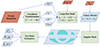 |
Fig. 1. Flow chart of the LIGER method in the ‘large-box’ mode (top row) and of the clustering analysis performed in this paper (bottom row). Inputs and outputs are displayed as red and blue parallelograms, respectively, while processes are shown as green rectangles. |
The updated particle positions are used to compute the matter overdensity in redshift space, δs. Eventually, the galaxy distribution in redshift space is obtained using

which matches Eq. (11) under two assumptions. Namely, (i)  ; (ii) we can neglect the linear perturbation of
  , where g denotes the determinant of the metric tensor9. The neglected terms are only relevant at scales larger than the Hubble radius (for more details, see Borzyszkowski et al. 2017). Aside from these minor contributions, Eq. (12) recovers the theoretical results obtained in Eq. (11).
3.2. N-body simulations
We considered a flat ΛCDM background cosmological model based on the results from the Planck mission (Planck Collaboration VI 2020) with the matter density parameter Ωm = 0.3158, baryon density parameter Ωb = 0.0508, and dimensionless Hubble constant h = 0.673. We also assumed that primordial scalar perturbations form a Gaussian random field with a linear power spectrum of power-law shape characterised by the spectral index ns = 0.966 and the amplitude As = 2.1 × 10⁻⁹ (defined at the wavenumber k* = 0.05 Mpc−1). We computed the matter transfer function using the CAMB code (Lewis & Bridle 2002).
In order to encompass the full EWSS within each of our simulation boxes, we studied structure formation within periodic cubic volumes with a comoving side length of Lbox = 12 h−1Gpc. As we are only interested in quasi-linear scales, we used second-order Lagrangian perturbation theory (2LPT) to build the dark-matter distribution that forms the input to LIGER. For this step, we applied the MUSIC code (Hahn & Abel 2011) to 10243 equal-mass particles, which initially form a regular Cartesian grid. Overdensities were computed with the classical cloud-in-cell scheme using the same grid. The gravitational potential was obtained by solving the Poisson equation with spectral methods (Hockney & Eastwood 1988).
We ran 35 independent N-body simulations and extracted four non-overlapping light cones from each of them, resulting in a total of Nmocks = 140 mock catalogues.
3.3. Euclid Hα galaxies
Applying Eq. (12) to Euclid requires knowledge of the functions b, ℰ, and 𝒬 for the Hα galaxies targeted by the EWSS. In the absence of accurate data, we assume that model 3 in Pozzetti et al. (2016) provides an accurate description of the luminosity function, as is suggested by recent observations (Bagley et al. 2020). Considering a flux limit of Flim = 2 × 10⁻¹⁶ erg cm−2 s−1 (Euclid Collaboration: Scaramella et al. 2022), we computed  by integrating the luminosity function and assuming a (uniform) completeness factor of 70%. We derived the evolution and magnification bias factors using Eqs. (9) and (10). Finally, for the linear bias coefficient, we adopted the linear relation b(z) = 1.46 + 0.68 (z − 1) obtained by fitting the data from Table 3 in Euclid Collaboration: Blanchard et al. (2020). All our results are presented in Fig. 2.
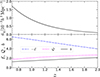 |
Fig. 2. Top: Background number density of galaxies in the EWSS as a function of redshift. Bottom: Corresponding evolution, magnification, and linear-bias parameters. |
3.4. Building the mock catalogues
For each of the 140 light cones, we built four different mock catalogues that progressively include an increasing number of relativistic RSDs. We first generated the galaxy distribution in real space (hereafter denoted by ℛ ). Second, we included the RSDs due to the peculiar velocities of the distant galaxies – that is, the terms depending on ve in Eqs. (4) and (7) – setting, however, 𝒬 and ℰ to zero in Eq. (12). We dubbed the corresponding catalogues 𝒱. Next, we considered all relativistic RSDs except those due to the observer peculiar velocity vo (from now on the 𝒢 mocks). Finally, we included all terms to generate the 𝒪 catalogues. In the latter set, we assumed that vo coincides with the peculiar velocity of the Sun as derived from the CMB dipole (Planck Collaboration I 2020).
To produce catalogues of discrete galaxies, we proceeded as follows. Based on δg, s and  , we first computed the expected number of galaxies, Ng, in each volume element of the light cone. We then drew from a Poisson distribution with mean Ng and randomly distributed the corresponding number of galaxies within the cell.
After taking all these steps, we obtained a full-sky galaxy catalogue covering the redshift range 0.9 < z < 1.8. In order to mimic the expected angular distribution of the EWSS, we masked 20° around the Galactic and Ecliptic planes as shown in Fig. 310. We measured clustering statistics in four tomographic redshift bins with boundaries z ∈ {0.9, 1.1, 1.3, 1.5, 1.8} and, particularly for the angular power spectrum, in a broader bin that covers the entire redshift range covered by the mock catalogues. The binning strategy used in this work has been chosen to reproduce that in Euclid Collaboration: Blanchard et al. (2020).
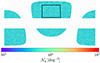 |
Fig. 3. Projected galaxy number counts for one of the 𝒱 mocks in the z ∈ (0.9, 1.1) redshift bin. The black lines enclose the region used in Sect. 8.2.1 as an example of a simply connected domain. |
3.5. Random catalogues
Estimating two-point statistics requires generating unclustered distributions of points with the same angular footprint and radial selection function as the actual galaxy data (see Sect. 6.1 and Sect. 7.1). We built a ‘random catalogue’ for each of our mocks in three steps. We first measured the mean galaxy number counts within radial shells of 20 h−1 Mpc width. We then interpolated the results with a cubic spline to obtain the cumulative redshift distribution of the galaxies. Finally, we used the inverse transform method to pick a redshift for the unclustered points, which are also assigned a random line-of-sight direction. The random catalogues contain five times more galaxies than the original light cones. These catalogues are smaller than those typically employed in power-spectrum estimation. Increasing the size of the random catalogue reduces the shot noise contribution to the statistical error of the power spectrum (Feldman et al. 1994). However, at the large scales considered in this work, the statistical error is dominated by the sample variance. Thus, using a smaller catalogue has minimal impact on our results while significantly reducing computational overhead.
4. Statistical methods
Given a clustering statistic, S, we want to understand whether the contribution of specific relativistic RSDs to the measured signal is detectable or not with the EWSS. For instance, the impact of the peculiar velocity of the observer can be quantified by comparing the clustering statistic extracted from our 𝒪 and 𝒢 mock catalogues. Similarly, by comparing the 𝒪 and 𝒱 light cones we can also study the relevance of the weak lensing contribution.
We denote with Dia the n-dimensional (column) data vector containing the measurements of the clustering statistics in a particular mock (characterised by the index, i) of type a ∈ {ℛ , 𝒱, 𝒢, 𝒪}. By taking the expectation over the 140 realisations, we computed the mean signal and the covariance matrix in the measurements,
![$$ \begin{aligned} {\boldsymbol{\mu }}_a&= \mathbb{E} [{\boldsymbol{D}}_i^{a}]\,,\end{aligned} $$](/articles/aa/full_html/2025/05/aa52480-24/aa52480-24-eq27.gif)
![$$ \begin{aligned} \mathsf{C }_a&= \mathbb{E} [({\boldsymbol{D}}_i^{a}-{\boldsymbol{\mu }}_a)({\boldsymbol{D}}_i^{a}-{\boldsymbol{\mu }}_a)^{\mathrm{T} }]\,. \end{aligned} $$](/articles/aa/full_html/2025/05/aa52480-24/aa52480-24-eq28.gif)
Based on the Fisher-information matrix, we can then estimate the S/N for the detection of the RSDs that are not included in the a mocks by using (see e.g. Sect. 3.3.3 in Borzyszkowski et al. 2017)

where we corrected for the bias of the inverse covariance matrix due to the finite number of realisations used to estimate it (Kaufman 1967; Hartlap et al. 2007).
Classical hypothesis testing based on the likelihood function provides another possibility to quantify the detectability of the different RSD terms. Assuming Gaussian errors, the likelihood that the dataset, Di𝒪, is drawn from a model, Ma, with signal μa is
![$$ \begin{aligned} L(M_a|{\boldsymbol{D}}_i^{{\mathcal{O} }}) \propto {\exp \left[-({\boldsymbol{D}}_i^{{\mathcal{O} }}-{\boldsymbol{\mu }}_a)^\mathrm{T} \,\mathsf C ^{-1}_a\,({\boldsymbol{D}}_i^{{\mathcal{O} }}-{\boldsymbol{\mu }}_a)/2\right]\over (2\,\pi )^{n/2}\det \mathsf{C }_a} \,. \end{aligned} $$](/articles/aa/full_html/2025/05/aa52480-24/aa52480-24-eq30.gif)
We use the term ‘model’ to indicate a prediction for S with fixed values of the parameters that describe the galaxy population and the underlying cosmology. No fitting of model parameters is considered here. Basically, a model corresponds to an infinite ensemble of mocks all including the same RSD terms (for instance, the 𝒢 mocks) and is described by the corresponding signal and noise covariance.
We now formulate the null hypothesis, ℋ0, that the Euclid data are a realisation of model Ma that does not include all RSD terms present in M𝒪. We want to test this assumption against the alternative hypothesis, ℋ1, that the data are drawn from M𝒪. The Neyman–Pearson lemma states that the likelihood-ratio test statistic
![$$ \begin{aligned} \lambda _i = 2\ln \left[{L(M_a|{\boldsymbol{D}}_i^{{\mathcal{O} }})\over L(M_{\mathcal{O} }|{\boldsymbol{D}}_i^{{\mathcal{O} }})}\right]\, \end{aligned} $$](/articles/aa/full_html/2025/05/aa52480-24/aa52480-24-eq31.gif)
provides the most powerful test for two simple hypotheses (i.e. with fixed model parameters). The null hypothesis is rejected with confidence level α if λi < ωα, where ωα is a real number such that the probability 𝒫(λi < ωα|ℋ0) = 1 − α. Under ℋ0, 𝒫(λi|ℋ0) is Gaussian, with a mean of m0 ≥ 0 and variance of s02 = 4m0 (see Appendix A in Borzyszkowski et al. 2017). Adopting a 95% confidence level, we thus obtain  . Similarly, under ℋ1, λi follows a Gaussian distribution with a mean of m = −(μ𝒪 − μa)TCa−1(μ𝒪 − μa)≤0 and variance of s2 = 4|m|. Therefore, ℋ0 is rejected in a fraction,
![$$ \begin{aligned} f_{95}={\frac{1}{2}}\left[1+\mathrm{erf} \left(\frac{\omega _{95}-m}{2\sqrt{2|m|}}\right)\right] ,\end{aligned} $$](/articles/aa/full_html/2025/05/aa52480-24/aa52480-24-eq33.gif)
of the realisations. If we neglect the small difference between the covariance matrices, we find that m = −m0 and s = s0 = 4m011. In this case, the separation between m and m0 expressed in units of the standard deviation of the distributions is  , which coincides with the S/N given in Eq. (15). The fraction of realisations in which the data reject ℋ0 is thus
 ![$ f_{95}=\{1+\mathrm{erf}[(\sqrt{m_0}-1.645)/\sqrt{2}]\}/2 $](/articles/aa/full_html/2025/05/aa52480-24/aa52480-24-eq35.gif) . We note that S/N = 1 gives f95 = 0.259, while f95 = 0.5 and 0.9 correspond to S/N = 1.645 and 2.93, respectively.
. We note that S/N = 1 gives f95 = 0.259, while f95 = 0.5 and 0.9 correspond to S/N = 1.645 and 2.93, respectively.
In the remainder of this paper, we apply these statistical tests to our mock Euclid light cones. As was anticipated at the beginning of this section, by comparing the 𝒪 and 𝒢 sets (hereafter 𝒪–𝒢 test) we assess the detectability of the RSDs generated by the peculiar velocity of the Sun. The goal here is to determine if and how often we manage to reject the null hypothesis that the 𝒪 data are drawn from an ensemble with vo = 0 . In addition, we apply the likelihood-ratio test to the 𝒪 and 𝒱 mocks (hereafter 𝒪–𝒱 test). In this case, we aim to quantify whether the EWSS can reject the null hypothesis that the influence of the integrated terms (dominated by the weak lensing contribution) on the clustering signal is negligible.
In order to perform these tests, we directly computed histograms of the values of λi derived from the 140 𝒪 mock catalogues. In all cases, we only used the C𝒪 covariance. This operation mimics what is usually done in the analysis of actual surveys, whereby the covariance is estimated from suites of mock catalogues and not changed with the theoretical models for which the likelihood is evaluated. We computed the S/N as
where the hat denotes estimates derived from the 140 mocks and determine f95 by counting the number of realisations in which λi < ω95. In order to facilitate the understanding of the likelihood-ratio test for two simple hypotheses, we present an illustrative example in Fig. 4.
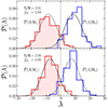 |
Fig. 4. Elucidatory example of the statistical test outlined in Sect. 4. In the top panel, the blue histogram on the right-hand side shows the distribution of the likelihood-ratio test statistic λ evaluated from the mock catalogues that do not include all relativistic RSDs (i.e. under the null hypothesis, ℋ0, which we try to rule out using the observed data). The red histogram on the left-hand side, instead, displays the distribution of λ in the mock light cones that account for all effects (i.e. under the alternative hypothesis, ℋ1). The solid and dashed curves represent Gaussian models for the histograms, as is described in the main text. The S/N is a measure of the separation between the two histograms in units of their RMS scatter. The shaded region highlights the realisations in which ℋ0 is ruled out at the 95% confidence level. The bottom panel only differs from the top one in the fact that the covariance matrix C𝒪 has been used to compute all likelihood functions. We use this approximation in the remainder of this paper. |
5. Angular power spectrum
In this section, we investigate the impact of relativistic RSDs on the angular power spectrum, Cℓ.
5.1. Estimator
We made use of the Hierarchical Equal Area isoLatitude Pixelisation (HEALPix; Górski et al. 2005; Zonca et al. 2019) algorithm12 to partition the sky into Npix = 12 × (1024)2 pixels. After dividing our mock light cones into multiple redshift bins, we computed the projected number counts of galaxies in each bin (indicated by the superscript i) and pixel, 𝒩gi(Ω). A sample sky map with the Euclid mask is shown in Fig. 3 using a cylindrical Cartesian co-ordinate system. The projected density contrast is then
where  denotes the average of 𝒩gi(Ω) over the solid angle subtended by the survey.
S/N from the 𝒪–𝒢 test applied to  with ℓ ∈ [1, 10].
We expanded the projected overdensities in spherical harmonics,
and measured the angular auto- and cross-power spectra using the pseudo-Cℓ (PCL) estimator (Peebles 1973; Loureiro et al. 2019)
where fsky denotes the fraction of the sky covered by the survey and wp is a correction factor due to the finite pixelisation of the sphere (see the HEALPix documentation for more details). In Appendix A, we present a validation test of our pipeline for producing the mock catalogues and measuring the angular power spectra.
5.2. Results
5.2.1. Peculiar velocity of the observer
In Eq. (11), a dipolar pattern is superimposed on the galaxy density contrast whenever the observer is not comoving with the cosmic expansion traced by matter (see also Gibelyou & Huterer 2012). Figure 5 displays how this kinematic dipole alters the angular power spectrum. Shown are the average and root-mean-square (RMS) scatter over the 140 mocks of the difference between the 𝒪 and 𝒢 spectra, which is  , for two different redshift bins. It is evident that, in a full-sky survey (red symbols), only the dipole (ℓ = 1) is affected by vo. On the other hand, the correction spreads over all the odd multipoles (ℓ = 3, 5, …) in our Euclid mocks due to the partial sky coverage of the catalogues. Expanding the projected overdensity in spherical harmonics (Eq. (21)) on a partial sky, where the base functions are no longer orthogonal, results in mode-mixing in the estimated angular power spectrum (Peebles 1973). Consequently, the dipole signal leaks into higher odd multipoles.
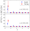 |
Fig. 5. Difference between the angular power spectra of the 𝒪 and 𝒢 mocks for a full-sky survey (red) and the EWSS (blue). The symbols indicate the mean signal, while the error bars show the standard deviation over the 140 realisations. |
In order to quantify how well the modification due to vo can be detected with the EWSS, we applied the 𝒪–𝒢 test introduced in Sect. 4 to the first ten multipoles. The resultant S/N values for the auto- and cross-spectra are shown in Table 1. For the tomographic redshift bins, the excess clustering induced by vo can be barely identified with a S/N of order one. This characteristic signature becomes much more discernible in the auto-correlation function evaluated after projecting the galaxies from the broad redshift interval z ∈ (0.9, 1.8). In this case, we obtain S/N = 2.1.
5.2.2. Weak lensing
Figure 6 displays the angular auto- and cross-power spectra extracted from the 𝒱 and 𝒪 mocks and re-binned with Δℓ = 5. The symbols show the average signal over the 140 realisations and the shaded region indicates the RMS scatter for the 𝒪 measurements. Since 2LPT at z ≃ 1 underestimates the non-linear matter power spectrum for wavenumbers k ≳ 0.05 h Mpc−1 (e.g. Taruya et al. 2018), we only consider harmonics of degree ℓ ≤ 120. The positioning of the panels is as in Tables 1 and 2. The cross-spectra between non-overlapping redshift bins are consistent with zero for the 𝒱 mocks and show a positive clustering signal for the 𝒪 catalogues. This difference is due to the integral terms in Eq. (11), in particular to the dominant weak lensing contribution. The auto-spectra also show enhanced clustering for the 𝒪 mocks. This is particularly evident in the bins that include galaxies with the highest redshifts.
The S/N values obtained with the 𝒪–𝒱 test are reported in Table 2. The detection of the lensing term is highly significant in the cross-correlations of well separated tomographic redshift bins and in all statistics involving the wide bin z ∈ (0.9, 1.8).
6. Two-point correlation function
The 2PCF is one of the most employed summary statistics to extract cosmological information from the large-scale structure of the Universe. In terms of the galaxy overdensity, it can be defined as (Peebles 1980)
where the brackets denote the average over an ensemble of realisations. In real space, we expect that δg is a statistically homogeneous and isotropic random field, so that ξg depends only on the magnitude of the separation between the points at which it is evaluated. Redshift-space distortions, however, break the translational and rotational symmetry of the 2PCF (as several terms in Eq. (11) depend on the line-of-sight direction with respect to the observer) into an azimuthal symmetry with respect to the line of sight. The 2PCF in redshift space thus depends on the shape and size of the (possibly non-Euclidean) triangle formed by the observer and the galaxy pair (Szalay et al. 1998; Matsubara 2000a).
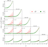 |
Fig. 6. Mean auto-and cross-angular power spectra extracted from the 𝒪 (red stars) and 𝒱 (green circles) mocks. The shaded region indicates the RMS scatter of the 𝒪 spectra. The panels are ordered as the entries in Tables 1 and 2. The cross-spectra of the tomographic redshift bins are multiplied by ten to improve the readability of the figure. |
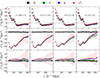 |
Fig. 7. Mean ℓ = 0, 2, and 4 multipoles of the 2PCF measured from the ℛ (black squares), 𝒱 (green circles), 𝒢 (blue crosses), and 𝒪 (red stars) mocks in the four tomographic redshift bins. The shaded areas highlight the RMS scatter among the 𝒪 light cones. |
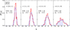 |
Fig. 8. PDF of the likelihood-ratio test statistic forthe 𝒪–𝒱 test applied to the multipoles of the 2PCF. |
6.1. Estimator
We used the Landy–Szalay (LS) estimator (Landy & Szalay 1993) implemented in the official Euclid code (Euclid Collaboration: De la Torre et al. in prep.), which adopts the midpoint co-ordinate system
and defines the pair-orientation angle, φ, through
where the hat denotes the unit vector; in other words,  13. After averaging over xm within the volume of interest, the code outputs an estimate of the 2PCF as a function of the galaxy separation and orientation with respect to the local line of sight,
  . It also computes the 2PCF Legendre multipoles
where ℒℓ(μ) denotes the Legendre polynomial of degree, ℓ. In what follows, we only consider the monopole (ℓ = 0), quadrupole (ℓ = 2), and hexadecapole (ℓ = 4) moments. These are the only non-vanishing moments in Kaiser’s GPP model and dominate the signal in general.
We originally estimated them in 500 equally spaced bins covering the range r ∈ [20 h−1 Mpc, Δx], where Δx denotes the comoving radial width of each redshift bin. This choice prevents the clustering signal from being dominated by galaxy pairs with particular angular separations, and thus limits window-function effects. We re-binned our results in different ways depending on our applications. For instance, we used ten equally separated bins in the range r ∈ [35 h−1 Mpc, Δx] for each multipole to perform the 𝒪–𝒢 and 𝒪–𝒱 tests.
6.2. Results
Figure 7 shows the mean multipoles of the 2PCF obtained from the different sets of mock catalogues. The shaded areas indicate the scatter for the 𝒪 light cones. The real-space monopole moment is positive at small separations, presents the baryonic-oscillation feature at r ≃ 100 h−1 Mpc, and crosses zero at r ≃ 125 h−1 Mpc, while  and
and  vanish as expected. Redshift-space distortions enhance the clustering signal in
  and generate a negative
  and a positive
  .
.
6.2.1. Peculiar velocity of the observer
The clustering signal extracted from the 𝒪 (red stars) and 𝒢 (blue crosses) mocks is hardly distinguishable at all scales in all tomographic redshift bins. This visual impression is confirmed by the 𝒪–𝒢 test, which consistently gives values of S/N ≤ 1 (see Table 3) for all redshift bins. At first sight, this appears to be at odds with the results by Bertacca et al. (2020) who predict stronger corrections due to vo. However, this study pushes the analysis to larger separations than ours and uses the bisector convention to define the line of sight to a galaxy pair (which changes the multipoles, e.g. Raccanelli et al. 2014; Reimberg et al. 2016).
S/N from the 𝒪–𝒱 and 𝒪–𝒢 tests for the multipoles of the 2PCF.
6.2.2. Weak lensing
Comparing the mean signal from the 𝒢 (blue crosses) and 𝒱 (green circles) multipoles, we notice that their difference increases with redshift and the pair separation. The contribution of the integral terms always enhances the clustering signal in the quadrupole and hexadecapole moments, but by an amount that is relatively small compared to the scatter in the measurements.
Performing the 𝒪–𝒱 test, we find that the S/N steadily grows from 0.81 to 2.48 from the lowest to the highest redshift bin (see Fig. 8 and Table 3). In the latter, the likelihood-ratio test manages to reject the velocity-only model for RSDs at the 95% confidence level in 78% of our mock catalogues.
7. Power spectrum
The galaxy power spectrum is the workhorse of cosmological-parameter inference. By analogy with Sect. 6, we introduced the covariance between two Fourier modes of the galaxy overdensity,  . If, in real space, δg(x) is a statistically homogeneous and isotropic field, then only the diagonal part of the covariance does not vanish, and the galaxy power spectrum, Pg(k), can be introduced using the relation
  . However, in redshift-space, where statistical homogeneity is lost, the covariance is not diagonal and the definition above does not apply (Zaroubi & Hoffman 1996). A different approach is thus needed.
The ‘local’ power spectrum, Ploc, was obtained by Fourier transforming the 2PCF with respect to r (Scoccimarro 2015),

In order to compress the clustering information into a set of functions of the wavenumber k, it is convenient to expand Ploc in Legendre polynomials of  and average over xm. These operations yield the so-called multipole moments of the power spectrum,

where V denotes the volume under consideration. In this section, we investigate the impact of relativistic RSDs on the power spectrum multipoles measured by the Euclid survey.
7.1. Estimator
In order to measure the multipoles of the power spectrum from a galaxy redshift survey, the ensemble average in Eq. (27) was replaced with a mean over a set of Fourier modes. We used the Yamamoto–Bianchi (Bianchi et al. 2015; Scoccimarro 2015) estimator implemented in the official Euclid code (Euclid Collaboration: Salvalaggio et al. in prep.).
Following Feldman et al. (1994, hereafter FKP), we first built the weighted galaxy overdensity,
![$$ \begin{aligned} F \left(\boldsymbol{x} \right)&= \frac{{ w} \left(\boldsymbol{x} \right)}{\sqrt{A}} \left[\,\widehat{n}_{\rm g} \left(\boldsymbol{x} \right) - \alpha \,\widehat{n}_{\rm r} ( \boldsymbol{x})\,\right]\,, \end{aligned} $$](/articles/aa/full_html/2025/05/aa52480-24/aa52480-24-eq60.gif)
by comparing the observed number density of galaxies  and its counterpart in the corresponding random catalogue,
  , introduced in Sect. 3.5. In order to minimise the variance of the measured multipoles, we adopted the weight function
![$$ \begin{aligned} w(\boldsymbol{x}) = \mathcal{I} (\boldsymbol{x}){\left[1+ {\overline{n}_{\rm g}}(x) \,\mathcal{P} _{0}\right]^{-1}}\,, \end{aligned} $$](/articles/aa/full_html/2025/05/aa52480-24/aa52480-24-eq63.gif)
where  denotes the mean density of galaxies, ℐ(x) is an indicator function that is one inside the volume under study and zero elsewhere, and the parameter 𝒫0 = 2 × 10⁴ h−3 Mpc3 gives an approximate value for the galaxy power spectrum at the scales of interest. The normalisation factor, A, was determined through the integral
  . Finally, the rescaling factor, α, was calculated using
The multipoles of the galaxy power spectrum with respect to the local line-of-sight direction could be directly estimated by computing (Yamamoto et al. 2000)
![$$ \begin{aligned} \hat{P}_\ell (k)&= (2\ell + 1)\int \int \int \left[F(\boldsymbol{x}_1)\,F(\boldsymbol{x}_2)\,\mathrm{e} ^{-\mathrm{i}\boldsymbol{k}\cdot (\boldsymbol{x_1}-\boldsymbol{x_2})}\right.\nonumber \\&\quad \left.\mathcal{L} _{\ell }\left(\hat{\boldsymbol{k}}\cdot {\hat{\boldsymbol{x}}_{\rm m}}\right)\;{\mathrm{d} }^3 x_1\;{\mathrm{d} }^3 x_2\;\frac{{\mathrm{d} }^2 \Omega _k}{4\pi }\right]-\hat{P}^\mathrm{SN}_\ell (k)\,, \end{aligned} $$](/articles/aa/full_html/2025/05/aa52480-24/aa52480-24-eq67.gif)
where Ωk denotes the solid angle in Fourier space and the shot noise contribution,  ,. is given by
Yamamoto et al. (2006) noticed that replacing the factor  with either
  or
or  in Eq. (33) results in a tremendous speed-up of the estimator. With this substitution – nowadays known as the LPP approximation – in fact,
  can be written as the product of two Fourier transforms that can be conveniently evaluated using the FFT algorithm (Beutler et al. 2014; Bianchi et al. 2015; Scoccimarro 2015); that is,
where
The official Euclid code that we used implements the faster estimator. It is worth stressing that Eqs. (33) and (35) define two different statistics, which generate different outputs when applied to wide-angle surveys (e.g. Samushia et al. 2015). For example, it has been demonstrated that the end-point convention distorts the values of the multipoles when compared to those evaluated using the midpoint convention (Reimberg et al. 2016; Castorina & White 2018).
As is shown in Figs. 7 and 9, the effects we investigate here leave their imprints on extremely large scales. For this reason, we computed FFTs within (periodic) cubic boxes with a side length of LFFT = 16 015 h−1 Mpc. That choice allows us to measure the power-spectrum multipoles down to the fundamental frequency kF = 4 × 10⁻⁴ h Mpc−1. We originally measured the multipoles with ℓ = 0, 2, and 4 within bins of size Δk = kF and we re-binned them in different ways depending on usage. For the 𝒪–𝒢 and 𝒪–𝒱 tests, we employed 12 equally spaced bins in the range k ∈ [0.4, 36]×10−3 h Mpc−1.
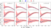 |
Fig. 9. Mean ℓ = 0, 2, and 4 multipoles of the power spectrum measured from the 𝒱 (green circles), 𝒢 (blue crosses), and 𝒪 (red stars) mocks in the four tomographic redshift bins. The shaded areas highlight the RMS scatter among the 𝒪 light cones. |
7.2. Results
The mean multipoles of the power spectrum measured from the different sets of mock catalogues are shown in Fig. 9 together with the RMS scatter from the 𝒪 set. The monopole moment shows the largest clustering amplitude and is measured with a high S/N, particularly for k > 2 × 10⁻² h Mpc−1. At the opposite extreme, the hexadecapole moment is suppressed by an order of magnitude with respect to P0 and its measurements are very noisy at all scales. The quadrupole moment has intermediate properties between the other two.
7.2.1. Peculiar velocity of the observer
By comparing the 𝒪 and 𝒢 spectra, we observe that the peculiar velocity of the observer modifies all multipoles at extremely large scales. For the monopole, this is consistent with the results presented by Elkhashab et al. (2021) who showed that a non-vanishing vo adds an oscillatory signal (damped with increasing k) to P0 with an oscillation frequency that increases with the characteristic redshift of the galaxy population. The coarse k-binning we adopt in this work does not reveal the details of the oscillations that then appear as a large-scale boost of the clustering amplitude in Fig. 9. Similar distortions are clearly noticeable also in P2 and P414. For the latter, in the first three tomographic bins, the corrected signal becomes negative at the largest scales probed here. The chances to detect these signatures with the EWSS are meagre, however, given the large scatter in the measurements at small wavenumbers. The S/N obtained with the 𝒪–𝒢 test is 1.3 at best (see Table 4) since the corrections due to vo are localised on very large scales where the measurement noise is large. Still, the enhanced clustering could bias measurements of the local-non-Gaussianity parameter, fNL, based on P0.
S/N from the 𝒪–𝒱 and 𝒪–𝒢 tests for the multipoles of the power spectrum.
7.2.2. Weak lensing
The difference between the multipoles extracted from the 𝒢 and 𝒱 mocks is minimal in the first three tomographic redshift bins but becomes more pronounced in the last one, particularly for ℓ = 2 and 4. This is consistent with the expectation that weak gravitational lensing should have a larger impact on the clustering of high-redshift galaxies. The 𝒪–𝒱 test closely mirrors the results we obtained for the 2PCF multipoles: the S/N for the detection of the integrated RSDs is always around one in the first three bins and jumps to 2.4 in the last one, for which the velocity-only model for RSDs is ruled out with 95% confidence in 78% of the realisations.
8. Perturbative models and survey window function
Up to this point, we have estimated the relative importance of various types of RSD in the forthcoming Euclid data by comparing the outputs of our different suites of mock catalogues. This approach deviates from what is usually done to interpret clustering measurements from redshift surveys. The standard procedure is to compare the observed summary statistics to analytical models (based on some flavour of perturbation theory) after accounting for the window function of the survey. In this section, we pursue this approach and assess whether Kaiser’s model for RSDs is accurate enough to describe the large-scale limit of the power-spectrum multipoles that Euclid will measure. We also present some interesting findings about the properties of the Euclid window function and the possibility of using disjoint patches of the sky in the same measurement of  .
.
8.1. The Kaiser model
In a seminal paper, Kaiser (1987) presented a theoretical model for the galaxy power spectrum in redshift space based on linear perturbation theory. The model only considers RSDs arising from the peculiar velocity gradient in Eq. (11). It also relies on the GPP approximation, according to which the lines of sight to all galaxies are parallel (as is expected for a small volume that is located at a large distance from the observer and that is thus seen under a narrow solid angle, i.e. under the distant-observer approximation). At a fixed cosmological redshift, it gives
where D+ denotes the linear growth factor for matter perturbations, Pm(k) is their linear power spectrum at z = 0,  is the line-of-sight direction, and

in terms of the (redshift-dependent) linear RSD parameter
This result can be generalised to model observations taken on a section of the past light cone (with volume Vs) of an observer, obtaining (to first approximation, e.g. Yamamoto et al. 1999; Pryer et al. 2022)
where
Going beyond this model requires dropping the GPP approximation and/or accounting for all the RSD terms appearing in Eq. (11). In order to correct the GPP predictions, Castorina & White (2018) propose expanding the multipoles of the wide-angle power spectrum in the parameter (k xm)−1. In this framework, the additional relativistic RSDs can then be treated perturbatively (Beutler et al. 2019; Castorina & Di Dio 2022; Noorikuhani & Scoccimarro 2023). The expansion in (k xm)−1, however, might become inaccurate for large angular separations. Another possible approach is to use the ‘spherical-Fourier-Bessel’ formalism that was introduced by Peebles (1973), extended to redshift space by Heavens & Taylor (1995), and applied to survey data in Percival et al. (2004). The inclusion of GR effects in this formalism is discussed in Yoo & Desjacques (2013), Bertacca et al. (2018), and Semenzato et al. (2025).
8.2. The window convolution and integral constraint
In order to compare theoretical models to the multipoles estimated from a survey, one needs to account for the fact that only a finite volume is observed. We can gain some insight into this issue by first considering the FKP power-spectrum estimator,  , derived under the GPP approximation. In this case, we obtain (Peacock 1991)
where  , and
, and  is the Fourier transform of the survey window function
The first term in Eq. (44) shows that the power-spectrum estimator mixes the contributions from Fourier modes that differ by less than the characteristic width of  , which is of the order of V−1/3 (in accordance with the uncertainty relation between conjugate Fourier variables). This has two main consequences: (i) the power spectrum is substantially distorted on large scales and (ii) additional anisotropy is generated on top of RSDs and the Alcock-Paczynski effect because of the spherical asymmetry of the window function. The second term in Eq. (44) gives the so-called (global) integral constraint, which arises from the assumption that the average density within the survey coincides with the actual mean density of the Universe. This term subtracts the actual power at k = 0, which leaks to larger wavenumbers because of the convolution with the window function, and thus enforces that Pobs(k) is zero for k = 0.
The considerations above can be generalised to the estimator for the power-spectrum multipoles introduced in Eq. (35) based on the LPP approximation. This gives (Beutler et al. 2014; Wilson et al. 2017; Beutler & McDonald 2021)
where Pg , ℓ′(k′) is computed under the GPP approximation,  denotes the multipole spectral moments of the window function, and 𝒲ℓℓ′(k, k′) are the elements of the so-called mixing matrix. The latter can be obtained from the multipoles, Qℓ(r), of the 2PCF of W(x) using
where the brackets denote the Wigner 3j symbols and jℓ is the spherical Bessel function of order ℓ. The functions Qℓ(r) could be directly estimated by counting pairs in the random catalogue (Wilson et al. 2017). However, it is computationally faster to obtain them using a Hankel transform,
evaluated with the FFTLog method (Hamilton 2000).
8.2.1. Disconnected patches
The EWSS avoids the ecliptic and Galactic planes and is thus composed of four disconnected regions (see Fig. 3). Considering all of them together would allow us to measure galaxy clustering on the largest possible scales. This is what we did in Sect. 7 to test the importance of the different RSD terms. However, this procedure differs from what is regularly done in ground-based surveys where northern and southern Galactic caps are analysed separately since each of them is subject to different angular systematics.
In order to contrast these approaches, in Fig. 11, we compare the functions Q0, Q2, and Q4 derived for the full Euclid footprint (solid lines) and for the simply connected patch covering 2565 deg2 displayed in Fig. 3 (dashed lines). In both cases, we consider the redshift bin z ∈ (1.1, 1.3). For separations of a few h−1 Mpc, the monopole moment approaches one while Q2 and Q4 are close to zero, reflecting the fact that Q(r) is nearly constant and isotropic for spatial lags that are well ’contained’ within the survey window function. On the other hand, Q(r) vanishes when r is larger than the maximum distance between two galaxies in the patch. In between these two asymptotic regimes, the 2PCF of the random catalogue becomes highly anisotropic with |Q2| and Q4 that assume values larger than Q0. The difference between the two survey footprints becomes evident on the largest scales: for instance, in the Euclid case, Q4 becomes negative when 1600 h−1 Mpc ≲ r ≲ 4400 h−1 Mpc and shows a prominent peak for r ≃ 5000 h−1 Mpc due to the presence of separate patches.
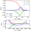 |
Fig. 11. 2PCF multipoles of the window function for the EWSS (solid) in the redshift bin z ∈ (1.1, 1.3) and for the single patch (dashed) shown in Fig. 3 in the same redshift range. The vertical lines indicate the characteristic length scale V1/3 for the two surveys. The bottom panel offers a more detailed view of the large-scale behaviour of the functions. |
In Fig. 12, we present all the elements of the resultant mixing matrices for the two different geometries considering the second tomographic bin z ∈ (1.1, 1.3). We fix k = 0.03 h Mpc−1 and plot 𝒲ℓℓ′(k, k′) as a function of k′. Each panel refers to a specific combination of ℓ and ℓ′. We plot the results for the Euclid footprint in black, while those for the connected patch are shown in red. As was expected, the most significant contributions come from k′=k but mixing takes place within a relatively broad range of wavenumbers. The matrix elements are always positive for ℓ = ℓ′ and show an oscillatory behaviour otherwise. These overall trends are present for both survey footprints. However, the results for the EWSS show high-frequency oscillations that are absent in the single patch case. This modulation can be traced back to presence of the peak at very large separations in the Qℓ functions presented in Fig. 11.
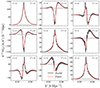 |
Fig. 12. Elements of the mixing matrix for the two surveys discussed in Fig. 11 evaluated at k = 0.03 h Mpc−1. |
8.2.2. Comparison with the LIGER mocks
We finally compare the theoretical model that accounts for the survey window and the integral constraint to the spectral multipoles extracted from our mock catalogues. For the sake of clarity, we summarise here how the theoretical prediction is computed: (i) we generated the linear matter power spectrum at z = 0 using the CAMB code; (ii) we utilised Kaiser’s model to obtain the galaxy power spectrum in redshift space and resorted to Eq. (42) in order to get the observed spectra on the past light cone; (iii) we computed the elements of the mixing matrix using the 2PCF multipoles estimated from the random catalogue of the mocks (see Eq. (47)); and (iv) we accounted for the survey window function and the integral constraint by making use of Eq. (46).
In Fig. 13, we compare the model (solid lines) to the measurements extracted from the 𝒱 mocks (symbols with error bars). As a reference, we also plot the theoretical predictions obtained without accounting for the finite-volume effects (dotted lines). Since we obtained similar results in all tomographic bins, we only show them for the interval z ∈ (1.1 , 1.3). The model and the measurements are in extremely good agreement at all wavenumbers, k > kC = 2 π/V1/3 (highlighted with a vertical dashed line). On larger scales, the quadrupole and hexadecapole moments show a small discrepancy, possibly due to wide-angle corrections missed by Kaiser’s model. A side note is in order here. The fact that Kaiser’s model nicely matches our 𝒱 mocks does not imply that it accounts for all RSDs generated by peculiar velocities. In fact, the 𝒱 catalogues were constructed by setting the magnification and evolution bias to zero, which automatically cancels some wide-angle effects. Anyway, the remarkable consistency we find validates the accuracy of the LIGER mock catalogues and demonstrates that the mixing-matrix formalism can be reliably used for surveys made of disconnected patches.
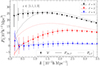 |
Fig. 13. Power-spectrum multipoles for the 𝒱 mocks in the redshift range z ∈ (1.1, 1.3). The mean and RMS scatter over the 140 mocks are displayed with squares and error bars, respectively. The solid and dotted lines show the theoretical predictions obtained with the Kaiser model (see Eq. (42)) with and without accounting for the window function of the EWSS (see Eq. (46)), respectively. The vertical dashed line marks the characteristic wavenumber, kC = 2 π/V1/3. |
Finally, we compared the theoretical model with the multipole moments extracted from the 𝒪 mocks, which mimic what will be observed by the actual Euclid mission. This way, we sought to assess the significance with which a theoretical model that accounts only for the velocity-gradient term can be ruled out due to the presence of additional RSDs in the data. Given the close match between the model and the numerical results obtained from the 𝒱 mocks, we obviously expected very similar results to those presented in Sect. 7.2.2. We employed the likelihood-ratio test and only considered wavenumbers k < kC grouped in 11 bins covering the range k ∈ [3.2, 36]×10−3 h Mpc−1 (slightly narrower than in Sect. 7.2.2). The resulting S/Ns for this (𝒪− Pobs) test are [1.3, 1.2, 1.5, 2.9] for the four tomographic bins listed in the same order as in Table 4. As was expected, these results are in good agreement with those deriving from the 𝒪–𝒱 test. This reinforces the conclusion that it is necessary to include at least the weak lensing corrections in order to obtain a good fit to the Euclid power-spectrum multipoles on scales k < 0.03 h Mpc−1.
9. Summary
The EWSS will measure redshifts and angular positions of nearly 30 million emission-line galaxies over a third of the sky and in the redshift range 0.9 ≲ z ≲ 1.8 (Laureijs et al. 2011). If observational systematic effects are kept under control, it will provide us with the opportunity to study galaxy clustering on unprecedentedly large scales. Theoretical considerations suggest that relativistic ‘projection’ effects alter the clustering signal we measure. In fact, galaxy observables (i.e. redshift, fluxes, and sky position) are influenced by the inhomogeneities that light encounters as it propagates from the galaxies to the observer. However, we construct maps of the galaxy distribution by assuming that galaxies populate an unperturbed model universe (for instance, in order to convert redshift into distances). This discrepancy leads to RSDs, which we need to model in order to interpret clustering data. While the leading effect generated by the relative peculiar velocities between the sources and the observer (Kaiser 1987) is regularly accounted for in all studies, additional contributions due to Doppler, gravitational lensing, Sachs–Wolfe, and time-delay type terms have mostly been neglected. The importance of these relativistic corrections is expected to grow as we investigate physical length scales approaching the Hubble radius. In this work, we make forecasts for their impact on different galaxy two-point statistics that will be measured from the EWSS; namely, the angular power spectrum, the multipole moments of the anisotropic 2PCF, and the multipole moments of the anisotropic power spectrum.
We used the LIGER method (summarised schematically in Fig. 1) to build 140 mock galaxy catalogues, each covering the whole footprint (and redshift range) of the EWSS and accounting for all relativistic RSDs up to the first order in the cosmological perturbations (see Fig. 3 for one example shown in projection). We studied the impact of different relativistic RSDs by turning on and off particular effects while producing the galaxy catalogues. In particular, for each of the 140 realisations, we generated the galaxy distribution in real space (ℛ ) and three different versions of its redshift-space counterpart. In the 𝒱 mocks, we basically only accounted for the spatial derivative of the peculiar velocity of the galaxies along the line of sight. In the 𝒢 catalogues, we added all the integral terms, which are dominated by the weak lensing signal (magnification bias and convergence). Finally, the 𝒪 mocks also include the distortions generated by a non-vanishing peculiar velocity of the observer, which we matched to the observed dipole temperature anisotropy of the cosmic microwave background. The 𝒪 catalogues mimic what will be obtained with Euclid using heliocentric redshifts. The ℛ , 𝒱, and 𝒢 mocks are useful tools for our investigation but do not correspond to anything15 that can be measured in reality. We note that our study automatically includes wide-angle effects induced by correlating pairs with large separations on the celestial sphere. On the other hand, we do not account for variations in the survey depth on the sky (which can generate a spurious clustering signal if not corrected for in the random catalogue) and redshift errors as we concentrate solely on the signal produced by relativistic RSDs.
We used the likelihood-ratio test to estimate the statistical significance with which the Euclid measurements could reject the null hypothesis that certain relativistic projection effects can be neglected in the theoretical models. In particular, given the summary statistics measured from the individual 𝒪 mocks, we have compared the likelihoods of the models obtained by averaging the clustering signal over all of the 𝒱, 𝒢, and 𝒪 catalogues with no tunable parameters. Our results can be summarised as follows.
(i) Angular power spectrum: The peculiar velocity of the observer noticeably increases the amplitude of the dipole (ℓ = 1), octupole (ℓ = 3), and dotriacontapole (ℓ = 5) signal measured in the heliocentric frame (Fig. 5). Statistically, this boost can be measured with a S/N of 2.1 for the redshift bin that encompasses the entire survey (Table 1) The combined effect of magnification bias and weak lensing convergence slightly increases the clustering signal for ℓ ≳ 50. This contribution is particularly evident in the broad redshift bin 0.9 < z < 1.8, where it is detectable with S/N = 5.4. Slightly smaller statistical significance (up to S/N = 4.5) is obtained by cross-correlating distant narrower bins (see Table 2). We note that the radial projection in the angular power spectrum strongly suppresses the contribution of the source peculiar velocities at small scales (large ℓ). Consequently, the weak-lensing contribution becomes the most dominant correction at these scales, in contrast to its behaviour in the 3D statistics.
(ii) Multipole moments of the 2PCF: The peculiar velocity of the observer introduces small modifications to the clustering signals and the likelihood-ratio test shows that the S/N for rejecting a model that assumes a comoving observer is always smaller than one. The weak lensing contribution amplifies the quadrupole and hexadecapole moments of the 2PCF at large scales (r > 150 h−1 Mpc) for z > 1.3 (see Fig. 7). The S/N of the combined contributions due to lensing and vo to the multipoles of the 2PCF grows with redshift and reaches 2.5 in the most distant tomographic bin we consider (1.5 < z < 1.8). Our results are in excellent agreement with the Fisher information-based S/N estimates provided by Euclid Collaboration: Jelic-Cizmek et al. (2024). These authors show that neglecting lensing magnification in the models systematically shifts the constraints on the cosmological parameters derived from the Euclid multipoles of the 2PCF. In the ΛCDM framework, the resulting bias is of the order of 0.4 – 0.7 standard deviations. Even larger biases affect model-independent estimates of the growth rate of structure.
(iii) Multipole moments of the power spectrum: The peculiar velocity of the observer imprints rather strong characteristic features on very large scales (k < 0.015 h Mpc−1) that are, however, difficult to detect with the EWSS due to the large statistical uncertainties of the measurements. The S/N is always of order one16 in all the tomographic bins we consider (Table 4). The weak gravitational lensing signal is mostly noticeable in the tomographic slice 1.5 < z < 1.8, where it can be detected with S/N = 2.4. In terms of the S/N of the different effects, considering the multipole moments of the power spectrum provides very similar results to those obtained from the 2PCF.
Since they are obtained by averaging the measurements of a given summary statistic over 140 mock catalogues, by construction, the models considered above are unbiased and perfectly account for wide-angle effects. In actual surveys, however, observational data are fit to theoretical predictions derived with some flavour of perturbation theory and based on assuming the LPP approximation. We thus repeated the likelihood-ratio test for the multipoles of the power spectrum by contrasting the mock-based predictions with a simple analytical model obtained combining the linear matter power spectrum with Kaiser’s model for RSDs. In order to compare it to the mock data accounting for the Euclid window function, we used the mixing-matrix formalism introduced in Eqs. (46) and (47). We find that the elements of the mixing matrix present high-frequency oscillations (Fig. 12) because the EWSS is made of four disconnected patches that we analyse simultaneously. The window-corrected theoretical model very closely matches the mean from the 𝒱 mocks. The striking agreement shown in Fig. 13 simultaneously demonstrates that (i) our mock catalogues are accurate, (ii) the mixing-matrix approach is also robust for surveys composed of multiple patches, and (iii) the power spectrum multipoles extracted from the 𝒱 mocks are not particularly affected by the wide-angle effects sourced by the velocity-gradient term. On the other hand, in the redshift bin 1.5 < z < 1.8, the window-corrected Kaiser model is rejected with S/N = 2.9 by the 𝒪 mocks that include all relativistic RSDs. This result reinforces the conclusion that the weak lensing term cannot be disregarded at high redshift and on large scales.
Related work based on the Euclid photometric sample and its cross-correlation with measurements of cosmic shear is presented in Euclid Collaboration: Lepori et al. (2022) and Euclid Collaboration: Tanidis et al. (2024).
In Eqs. (4) and (5), we are neglecting the fact that the co-ordinate time does not coincide with the proper time of the observer in an inhomogenous universe. This only affects the mean number density and has no impact on the density contrast (Bertacca et al. 2020; Grimm & Yoo 2021).
The synchronous comoving galaxy overdensity is related to its Poisson gauge counterpart,  , via
, via  (e.g. Jeong et al. 2012).
A code implementation in C is publicly available at https://astro.uni-bonn.de/~porciani/LIGER/.
Relativistic species, such as massive neutrinos, generate anisotropic stress (a difference between the metric perturbations Φ − Ψ ≠ 0). Their impact on the power spectrum from the EWSS is discussed in Euclid Collaboration: Archidiacono et al. (2025) and is irrelevant for the scales considered in this work.
At linear order, the perturbation of  corresponds to the trace of the metric given in Eq. (3).
We did not simulate direction-dependent incompleteness (for instance due to Galactic extinction, Euclid Collaboration: Monaco et al. in prep.) which affects the clustering summary statistics at large scales. These effects can be mitigated when estimating the clustering statistics (e.g. Burden et al. 2017; Paviot et al. 2022)
The HEALPix/healpy software package is available in http://healpix.sourceforge.net.
Many studies of wide-angle effects use a different convention that defines the line of sight as the direction bisecting the angle formed by the two galaxies (e.g. Szalay et al. 1998; Matsubara 2000a; Szapudi 2004; Raccanelli et al. 2010; Samushia et al. 2012; Bertacca et al. 2012). For small angles, this differs from the midpoint method at 𝒪(φ2).
A derivation of the impact of vo on all multipoles is presented in (Elkhashab et al. 2024).
The 𝒢 catalogues correspond to what a comoving observer would measure but this does not coincide with the galaxy maps obtained by correcting the galaxy redshifts measured by a non-comoving observer (Elkhashab et al. 2024).
Higher significance is found either considering wider redshift bins (Elkhashab et al. 2021) or using dedicated statistics (Elkhashab et al. 2024).
Acknowledgments
DB and MYE acknowledge support from the COSMOS network through the ASI (Italian Space Agency) Grants 2016-24-H.0, 2016-24-H.1-2018 and 2020-9-HH.0. MYE and DB acknowledge funding from the Italian Ministry of Education, University and Research (MIUR) through the “Dipartimenti di eccellenza” project “Science of the Universe”. The Euclid Consortium acknowledges the European Space Agency and a number of agencies and institutes that have supported the development of Euclid, in particular the Agenzia Spaziale Italiana, the Austrian Forschungsförderungsgesellschaft funded through BMK, the Belgian Science Policy, the Canadian Euclid Consortium, the Deutsches Zentrum für Luft- und Raumfahrt, the DTU Space and the Niels Bohr Institute in Denmark, the French Centre National d’Etudes Spatiales, the Fundação para a Ciência e a Tecnologia, the Hungarian Academy of Sciences, the Ministerio de Ciencia, Innovación y Universidades, the National Aeronautics and Space Administration, the National Astronomical Observatory of Japan, the Netherlandse Onderzoekschool Voor Astronomie, the Norwegian Space Agency, the Research Council of Finland, the Romanian Space Agency, the State Secretariat for Education, Research, and Innovation (SERI) at the Swiss Space Office (SSO), and the United Kingdom Space Agency. A complete and detailed list is available on the Euclid web site (https://www.euclid-ec.org).
References
- Bagley, M. B., Scarlata, C., Mehta, V., et al. 2020, ApJ, 897, 98 [NASA ADS] [CrossRef] [Google Scholar]
- Bahr-Kalus, B., Bertacca, D., Verde, L., & Heavens, A. 2021, JCAP, 11, 027 [Google Scholar]
- Bertacca, D. 2015, Classical Quantum Gravity, 32, 195011 [Google Scholar]
- Bertacca, D. 2020, Int. J. Mod. Phys. D, 29, 2050085 [Google Scholar]
- Bertacca, D., Maartens, R., Raccanelli, A., & Clarkson, C. 2012, JCAP, 10, 025 [Google Scholar]
- Bertacca, D., Raccanelli, A., Bartolo, N., et al. 2018, Phys. Rev. D, 97, 023531 [Google Scholar]
- Bertacca, D., Ricciardone, A., Bellomo, N., et al. 2020, Phys. Rev. D, 101, 103513 [Google Scholar]
- Beutler, F., & McDonald, P. 2021, JCAP, 11, 031 [Google Scholar]
- Beutler, F., Saito, S., Seo, H.-J., et al. 2014, MNRAS, 443, 1065 [NASA ADS] [CrossRef] [Google Scholar]
- Beutler, F., Castorina, E., & Zhang, P. 2019, JCAP, 03, 040 [Google Scholar]
- Bianchi, D., Gil-Marín, H., Ruggeri, R., & Percival, W. J. 2015, MNRAS, 453, L11 [NASA ADS] [CrossRef] [Google Scholar]
- Bonvin, C., & Durrer, R. 2011, Phys. Rev. D, 84, 063505 [NASA ADS] [CrossRef] [Google Scholar]
- Borzyszkowski, M., Bertacca, D., & Porciani, C. 2017, MNRAS, 471, 3899 [NASA ADS] [CrossRef] [Google Scholar]
- Breton, M.-A., Rasera, Y., Taruya, A., Lacombe, O., & Saga, S. 2019, MNRAS, 483, 2671 [NASA ADS] [CrossRef] [Google Scholar]
- Breton, M.-A., de la Torre, S., & Piat, J. 2022, A&A, 661, A154 [NASA ADS] [CrossRef] [EDP Sciences] [Google Scholar]
- Broadhurst, T. J., Taylor, A. N., & Peacock, J. A. 1995, ApJ, 438, 49 [Google Scholar]
- Burden, A., Padmanabhan, N., Cahn, R. N., White, M. J., & Samushia, L. 2017, JCAP, 03, 001 [Google Scholar]
- Camera, S., Maartens, R., & Santos, M. G. 2015, MNRAS, 451, L80 [NASA ADS] [CrossRef] [Google Scholar]
- Castorina, E., & Di Dio, E. 2022, JCAP, 01, 061 [CrossRef] [Google Scholar]
- Castorina, E., & White, M. 2018, MNRAS, 476, 4403 [NASA ADS] [Google Scholar]
- Castorina, E., Hand, N., Seljak, U., et al. 2019, JCAP, 09, 010 [Google Scholar]
- Challinor, A., & Lewis, A. 2011, Phys. Rev. D, 84, 043516 [NASA ADS] [CrossRef] [Google Scholar]
- Cole, S., Percival, W. J., Peacock, J. A., et al. 2005, MNRAS, 362, 505 [Google Scholar]
- Di Dio, E., Montanari, F., Lesgourgues, J., & Durrer, R. 2013, JCAP, 11, 044 [CrossRef] [Google Scholar]
- Eisenstein, D. J., Zehavi, I., Hogg, D. W., et al. 2005, ApJ, 633, 560 [Google Scholar]
- Elkhashab, M. Y., Porciani, C., & Bertacca, D. 2021, MNRAS, 509, 1626 [NASA ADS] [CrossRef] [Google Scholar]
- Elkhashab, M. Y., Porciani, C., & Bertacca, D. 2024, ArXiv e-prints [arXiv:2412.03953] [Google Scholar]
- Euclid Collaboration (Blanchard, A. et al.) 2020, A&A, 642, A191 [NASA ADS] [CrossRef] [EDP Sciences] [Google Scholar]
- Euclid Collaboration (Borlaff, A. S. et al.) 2022, A&A, 657, A92 [NASA ADS] [CrossRef] [EDP Sciences] [Google Scholar]
- Euclid Collaboration (Lepori, F. et al.) 2022, A&A, 662, A93 [NASA ADS] [CrossRef] [EDP Sciences] [Google Scholar]
- Euclid Collaboration (Scaramella, R. et al.) 2022, A&A, 662, A112 [NASA ADS] [CrossRef] [EDP Sciences] [Google Scholar]
- Euclid Collaboration (Schirmer, M. et al.) 2022, A&A, 662, A92 [NASA ADS] [CrossRef] [EDP Sciences] [Google Scholar]
- Euclid Collaboration (Jelic-Cizmek, G. et al.) 2024, A&A, 685, A167 [NASA ADS] [CrossRef] [EDP Sciences] [Google Scholar]
- Euclid Collaboration (Tanidis, K. et al.) 2024, A&A, 683, A17 [NASA ADS] [CrossRef] [EDP Sciences] [Google Scholar]
- Euclid Collaboration (Archidiacono, M. et al.) 2025, A&A, 693, A58 [NASA ADS] [CrossRef] [EDP Sciences] [Google Scholar]
- Euclid Collaboration (Mellier, Y. et al.) 2025, A&A, 697, A1 [Google Scholar]
- Feldman, H. A., Kaiser, N., & Peacock, J. A. 1994, ApJ, 426, 23 [Google Scholar]
- Foglieni, M., Pantiri, M., Di Dio, E., & Castorina, E. 2023, Phys. Rev. Lett., 131, 111201 [Google Scholar]
- Gibelyou, C., & Huterer, D. 2012, MNRAS, 427, 1994 [NASA ADS] [CrossRef] [Google Scholar]
- Górski, K. M., Hivon, E., Banday, A. J., et al. 2005, ApJ, 622, 759 [Google Scholar]
- Grimm, N., & Yoo, J. 2021, Phys. Rev. D, 104, 083548 [Google Scholar]
- Hahn, O., & Abel, T. 2011, MNRAS, 415, 2101 [Google Scholar]
- Hamilton, A. J. S. 1998, in The Evolving Universe, ed. D. Hamilton, Astrophys. Space Sci. Libr., 231, 185 [Google Scholar]
- Hamilton, A. J. S. 2000, MNRAS, 312, 257 [NASA ADS] [CrossRef] [Google Scholar]
- Hamilton, A. J. S. 2005, ArXiv e-prints [arXiv:astro-ph/0503604] [Google Scholar]
- Hamilton, A. J. S., & Culhane, M. 1996, MNRAS, 278, 73 [Google Scholar]
- Hartlap, J., Simon, P., & Schneider, P. 2007, A&A, 464, 399 [NASA ADS] [CrossRef] [EDP Sciences] [Google Scholar]
- Heavens, A. F., & Taylor, A. N. 1995, MNRAS, 275, 483 [NASA ADS] [Google Scholar]
- Hockney, R. W., & Eastwood, J. W. 1988, Computer simulation using particles (CRC Press) [Google Scholar]
- Hui, L., & Greene, P. B. 2006, Phys. Rev. D, 73, 123526 [NASA ADS] [CrossRef] [Google Scholar]
- Hui, L., Gaztañaga, E., & LoVerde, M. 2007, Phys. Rev. D, 76, 103502 [NASA ADS] [CrossRef] [Google Scholar]
- Hui, L., Gaztañaga, E., & LoVerde, M. 2008, Phys. Rev. D, 77, 063526 [NASA ADS] [CrossRef] [Google Scholar]
- Jelic-Cizmek, G., Lepori, F., Bonvin, C., & Durrer, R. 2021, JCAP, 04, 055 [NASA ADS] [CrossRef] [Google Scholar]
- Jeong, D., Schmidt, F., & Hirata, C. M. 2012, Phys. Rev. D, 85, 023504 [NASA ADS] [CrossRef] [Google Scholar]
- Kaiser, N. 1987, MNRAS, 227, 1 [Google Scholar]
- Kaufman, G. M. 1967, Report N. 6710, Center for Operations Research and Econometrics. Catholic University of Louvain. Heverlee, Belgium [Google Scholar]
- Landy, S. D., & Szalay, A. S. 1993, ApJ, 412, 64 [Google Scholar]
- Laureijs, R., Amiaux, J., Arduini, S., et al. 2011, ArXiv e-prints [arXiv:1110.3193] [Google Scholar]
- Lewis, A., & Bridle, S. 2002, Phys. Rev. D, 66, 103511 [Google Scholar]
- Loureiro, A., Moraes, B., Abdalla, F. B., et al. 2019, MNRAS, 485, 326 [NASA ADS] [CrossRef] [Google Scholar]
- Maciaszek, T., Ealet, A., Gillard, W., et al. 2022, in Space Telescopes and Instrumentation 2022: Optical, Infrared, and Millimeter Wave, eds. L. E. Coyle, M. D. Perrin, & S. Matsuura, SPIE, 12180, 613 [Google Scholar]
- Matsubara, T. 2000a, ApJ, 535, 1 [Google Scholar]
- Matsubara, T. 2000b, ApJ, 537, L77 [NASA ADS] [CrossRef] [Google Scholar]
- Noorikuhani, M., & Scoccimarro, R. 2023, Phys. Rev. D, 107, 083528 [Google Scholar]
- Pápai, P., & Szapudi, I. 2008, MNRAS, 389, 292 [CrossRef] [Google Scholar]
- Paviot, R., de la Torre, S., de Mattia, A., et al. 2022, MNRAS, 512, 1341 [NASA ADS] [CrossRef] [Google Scholar]
- Peacock, J. A. 1991, MNRAS, 253, 1 [Google Scholar]
- Peacock, J. A., Cole, S., Norberg, P., et al. 2001, Nature, 410, 169 [Google Scholar]
- Peebles, P. J. E. 1973, ApJ, 185, 413 [Google Scholar]
- Peebles, P. J. E. 1980, The Large-Scale Structure of the Universe (Princeton University Press) [Google Scholar]
- Percival, W. J., Burkey, D., Heavens, A., et al. 2004, MNRAS, 353, 1201 [NASA ADS] [CrossRef] [Google Scholar]
- Planck Collaboration I. 2020, A&A, 641, A1 [NASA ADS] [CrossRef] [EDP Sciences] [Google Scholar]
- Planck Collaboration VI. 2020, A&A, 641, A6 [NASA ADS] [CrossRef] [EDP Sciences] [Google Scholar]
- Pozzetti, L., Hirata, C. M., Geach, J. E., et al. 2016, A&A, 590, A3 [NASA ADS] [CrossRef] [EDP Sciences] [Google Scholar]
- Pryer, D., Smith, R. E., Booth, R., et al. 2022, JCAP, 08, 019 [Google Scholar]
- Raccanelli, A., Samushia, L., & Percival, W. J. 2010, MNRAS, 409, 1525 [NASA ADS] [CrossRef] [Google Scholar]
- Raccanelli, A., Bertacca, D., Doré, O., & Maartens, R. 2014, JCAP, 08, 022 [Google Scholar]
- Raccanelli, A., Montanari, F., Bertacca, D., Doré, O., & Durrer, R. 2016, JCAP, 05, 009 [Google Scholar]
- Raccanelli, A., Bertacca, D., Jeong, D., Neyrinck, M. C., & Szalay, A. S. 2018, Phys. Dark Univ., 19, 109 [Google Scholar]
- Reimberg, P., Bernardeau, F., & Pitrou, C. 2016, JCAP, 01, 048 [Google Scholar]
- Samushia, L., Percival, W. J., & Raccanelli, A. 2012, MNRAS, 420, 2102 [Google Scholar]
- Samushia, L., Branchini, E., & Percival, W. J. 2015, MNRAS, 452, 3704 [Google Scholar]
- Sargent, W. L. W., & Turner, E. L. 1977, ApJ, 212, L3 [NASA ADS] [CrossRef] [Google Scholar]
- Scoccimarro, R. 2015, Phys. Rev. D, 92, 083532 [NASA ADS] [CrossRef] [Google Scholar]
- Semenzato, F., Bertacca, D., & Raccanelli, A. 2025, Phys. Rev. D, 111, 023522 [Google Scholar]
- Szalay, A. S., Matsubara, T., & Landy, S. D. 1998, ApJ, 498, L1 [NASA ADS] [CrossRef] [Google Scholar]
- Szapudi, I. 2004, ApJ, 614, 51 [NASA ADS] [CrossRef] [Google Scholar]
- Tansella, V., Jelic-Cizmek, G., Bonvin, C., & Durrer, R. 2018, JCAP, 10, 032 [Google Scholar]
- Taruya, A., Nishimichi, T., & Jeong, D. 2018, Phys. Rev. D, 98, 103532 [Google Scholar]
- Wilson, M. J., Peacock, J. A., Taylor, A. N., & de la Torre, S. 2017, MNRAS, 464, 3121 [Google Scholar]
- Yamamoto, K., Nishioka, H., & Suto, Y. 1999, ApJ, 527, 488 [Google Scholar]
- Yamamoto, K., Nishioka, H., & Taruya, A. 2000, ArXiv e-prints [arXiv:astro-ph/0012433] [Google Scholar]
- Yamamoto, K., Nakamichi, M., Kamino, A., Bassett, B. A., & Nishioka, H. 2006, PASJ, 58, 93 [Google Scholar]
- Yoo, J., & Desjacques, V. 2013, Phys. Rev. D, 88, 023502 [Google Scholar]
- Yoo, J., Fitzpatrick, A., & Zaldarriaga, M. 2009, Phys. Rev. D, 80, 083514 [NASA ADS] [CrossRef] [Google Scholar]
- Zaroubi, S., & Hoffman, Y. 1996, ApJ, 462, 25 [Google Scholar]
- Zonca, A., Singer, L., Lenz, D., et al. 2019, J. Open Source Softw., 4, 1298 [Google Scholar]
Appendix A: Validation of the LIGER method
The calculation of the galaxy angular power spectrum with relativistic RSDs (but excluding corrections due to  and considering constant values of b and 𝒬) has been integrated into the CAMB and CLASS codes (Di Dio et al. 2013). Here, we validate the LIGER method by comparing the mean of the angular power spectra estimated from our ℛ and 𝒢 mock catalogues to the output of CAMB. For simplicity, we perform the comparison for a full-sky survey and we provide the density-weighted average of the b and 𝒬 functions as input to CAMB. Figure A.1 shows that the two methods agree to better than 1% for ℓ ≲ 90 for the tomographic bin z ∈ (1.1, 1.3). The loss of power of the mock catalogues at higher multipoles is irrelevant for our study (which focuses on larger scales) and can be attributed to the coarse spatial resolution of the input 2LPT simulations (see Sect. 3.2). Similar results are obtained for the other redshift bins.
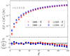 |
Fig. A.1. Top: Mean angular power spectra estimated from our mock catalogues (squares with RMS error bars) for the ℛ (red) and 𝒢 (blue) suites are compared to the corresponding output from the CAMB code (crosses). All spectra were binned using intervals Δℓ = 5. Bottom: Relative difference between the spectra (error bars here indicate the standard error of the mean). |
All Tables
All Figures
|
Fig. 1. Flow chart of the LIGER method in the ‘large-box’ mode (top row) and of the clustering analysis performed in this paper (bottom row). Inputs and outputs are displayed as red and blue parallelograms, respectively, while processes are shown as green rectangles. |
| In the text | |
|
Fig. 2. Top: Background number density of galaxies in the EWSS as a function of redshift. Bottom: Corresponding evolution, magnification, and linear-bias parameters. |
| In the text | |
|
Fig. 3. Projected galaxy number counts for one of the 𝒱 mocks in the z ∈ (0.9, 1.1) redshift bin. The black lines enclose the region used in Sect. 8.2.1 as an example of a simply connected domain. |
| In the text | |
|
Fig. 4. Elucidatory example of the statistical test outlined in Sect. 4. In the top panel, the blue histogram on the right-hand side shows the distribution of the likelihood-ratio test statistic λ evaluated from the mock catalogues that do not include all relativistic RSDs (i.e. under the null hypothesis, ℋ0, which we try to rule out using the observed data). The red histogram on the left-hand side, instead, displays the distribution of λ in the mock light cones that account for all effects (i.e. under the alternative hypothesis, ℋ1). The solid and dashed curves represent Gaussian models for the histograms, as is described in the main text. The S/N is a measure of the separation between the two histograms in units of their RMS scatter. The shaded region highlights the realisations in which ℋ0 is ruled out at the 95% confidence level. The bottom panel only differs from the top one in the fact that the covariance matrix C𝒪 has been used to compute all likelihood functions. We use this approximation in the remainder of this paper. |
| In the text | |
|
Fig. 5. Difference between the angular power spectra of the 𝒪 and 𝒢 mocks for a full-sky survey (red) and the EWSS (blue). The symbols indicate the mean signal, while the error bars show the standard deviation over the 140 realisations. |
| In the text | |
|
Fig. 6. Mean auto-and cross-angular power spectra extracted from the 𝒪 (red stars) and 𝒱 (green circles) mocks. The shaded region indicates the RMS scatter of the 𝒪 spectra. The panels are ordered as the entries in Tables 1 and 2. The cross-spectra of the tomographic redshift bins are multiplied by ten to improve the readability of the figure. |
| In the text | |
|
Fig. 7. Mean ℓ = 0, 2, and 4 multipoles of the 2PCF measured from the ℛ (black squares), 𝒱 (green circles), 𝒢 (blue crosses), and 𝒪 (red stars) mocks in the four tomographic redshift bins. The shaded areas highlight the RMS scatter among the 𝒪 light cones. |
| In the text | |
|
Fig. 8. PDF of the likelihood-ratio test statistic forthe 𝒪–𝒱 test applied to the multipoles of the 2PCF. |
| In the text | |
|
Fig. 9. Mean ℓ = 0, 2, and 4 multipoles of the power spectrum measured from the 𝒱 (green circles), 𝒢 (blue crosses), and 𝒪 (red stars) mocks in the four tomographic redshift bins. The shaded areas highlight the RMS scatter among the 𝒪 light cones. |
| In the text | |
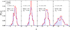 |
Fig. 10. Similar to Fig. 8 using the power spectrum multipoles as the data vector. |
| In the text | |
|
Fig. 11. 2PCF multipoles of the window function for the EWSS (solid) in the redshift bin z ∈ (1.1, 1.3) and for the single patch (dashed) shown in Fig. 3 in the same redshift range. The vertical lines indicate the characteristic length scale V1/3 for the two surveys. The bottom panel offers a more detailed view of the large-scale behaviour of the functions. |
| In the text | |
|
Fig. 12. Elements of the mixing matrix for the two surveys discussed in Fig. 11 evaluated at k = 0.03 h Mpc−1. |
| In the text | |
|
Fig. 13. Power-spectrum multipoles for the 𝒱 mocks in the redshift range z ∈ (1.1, 1.3). The mean and RMS scatter over the 140 mocks are displayed with squares and error bars, respectively. The solid and dotted lines show the theoretical predictions obtained with the Kaiser model (see Eq. (42)) with and without accounting for the window function of the EWSS (see Eq. (46)), respectively. The vertical dashed line marks the characteristic wavenumber, kC = 2 π/V1/3. |
| In the text | |
|
Fig. A.1. Top: Mean angular power spectra estimated from our mock catalogues (squares with RMS error bars) for the ℛ (red) and 𝒢 (blue) suites are compared to the corresponding output from the CAMB code (crosses). All spectra were binned using intervals Δℓ = 5. Bottom: Relative difference between the spectra (error bars here indicate the standard error of the mean). |
| In the text | |
Current usage metrics show cumulative count of Article Views (full-text article views including HTML views, PDF and ePub downloads, according to the available data) and Abstracts Views on Vision4Press platform.
Data correspond to usage on the plateform after 2015. The current usage metrics is available 48-96 hours after online publication and is updated daily on week days.
Initial download of the metrics may take a while.