| Issue |
A&A
Volume 694, February 2025
|
|
|---|---|---|
| Article Number | A54 | |
| Number of page(s) | 13 | |
| Section | Stellar atmospheres | |
| DOI | https://doi.org/10.1051/0004-6361/202452385 | |
| Published online | 31 January 2025 | |
Structure formation in O-type stars and Wolf–Rayet stars
1
Institute of Astronomy, KU Leuven,
Celestijnenlaan 200D,
3001
Leuven,
Belgium
2
Anton Pannekoek Institute for Astronomy, University of Amsterdam,
1090GE
Amsterdam,
The Netherlands
★ Corresponding author; cassandra.vandersijpt@kuleuven.be
Received:
26
September
2024
Accepted:
10
January
2025
Context. Turbulent small-scale structures in the envelopes and winds of massive stars have long been suggested as the cause for excessive line broadening in the spectra of these stars that could not be explained by other mechanisms such as thermal broadening. However, while these structures are also seen in recent radiation-hydrodynamical simulations, their origin, particularly in the envelope, has not been extensively studied.
Aims. We study the origin of structures seen in 2D radiation-hydrodynamical unified stellar atmosphere and wind simulations of O stars and Wolf–Rayet stars. Particularly, we study whether the structure growth in the simulations is consistent with sub-surface convection, as is commonly assumed to be the origin of this turbulence.
Methods. Using a linear stability analysis of the optically thick, radiation-pressure dominated envelopes of massive stars, we identified multiple instabilities that could be driving structure growth. We quantified the structure growth in the non-linear simulations of O stars and Wolf–Rayet stars by computing density power spectra and tracking their temporal evolution. Then, we compared these results to the analytical results from the stability analysis to distinguish between the different instabilities.
Results. The stability analysis leads to two possible instabilities: the convective instability and an acoustic instability that is a local variant of so-called strange modes. Analytic expressions for the growth rates of these different instabilities are found. In particular, strong radiative diffusion damps the growth rate ω of the convective instability in this regime leading to a distinct ω ∼ 1/k2 dependence on wavenumber k. From our power spectra analysis of the simulations, however, we find that structure growth rather increases with k – tentatively as ω ~ √k.
Conclusions. Our results suggest that, contrary to what is commonly assumed, structures in luminous O and Wolf–Rayet star envelopes do not primarily develop from the sub-surface convective instability. Rather the growth seems compatible with either the acoustic instability in the radiation-dominated regime or with Rayleigh-Taylor type instabilities, although the exact origin remains inconclusive for now.
Key words: hydrodynamics / instabilities / turbulence / stars: atmospheres / stars: winds, outflows / stars: Wolf–Rayet
© The Authors 2025
 Open Access article, published by EDP Sciences, under the terms of the Creative Commons Attribution License (https://creativecommons.org/licenses/by/4.0), which permits unrestricted use, distribution, and reproduction in any medium, provided the original work is properly cited.
This article is published in open access under the Subscribe to Open model. Subscribe to A&A to support open access publication.
1 Introduction
Generally, massive stars are believed to have convective cores and smooth radiative envelopes. The current unified model atmosphere codes, covering the sub-surface layers up to the wind outflow simultaneously, assume the atmosphere to be spherically symmetric, stationary, and in radiative equilibrium in order to model it in 1D (see for example, FASTWIND; Santolaya-Rey et al. 1997; Puls et al. 2005, 2020; Sundqvist & Puls 2018, CMFGEN; Hillier & Miller 1998; Hillier & Lanz 2001, POWR; Gräfener et al. 2002; Hamann & Gräfener 2004; Sander et al. 2012). Nonetheless, there have been observational and theoretical indications showing that the assumption of a smooth envelope and wind may not hold.
Particularly, excessive line broadening in O stars has been linked to “macroturbulence,” large-scale motions of clumps near the surface (Conti & Ebbets 1977; Howarth et al. 1997; Simón-Díaz et al. 2017). Furthermore, the winds of these stars are believed to be clumped as well (Eversberg et al. 1998; Puls et al. 2006; Oskinova et al. 2007; Sundqvist et al. 2010; Šurlan et al. 2012; Hawcroft et al. 2021; Rubio-Díez et al. 2022; Brands et al. 2022). This implies that both the envelope and the wind of these O stars are structured instead of smooth. Also for classical Wolf–Rayet (WR) stars, which are believed to be evolved O stars, their envelopes and winds were shown to be structured (Moffat et al. 1988; Lepine 1994; Dessart & Owocki 2002; Crowther 2007; Michaux et al. 2014). Moreover, recent multi-dimensional modeling efforts (Jiang et al. 2015; Moens et al. 2022b; Debnath et al. 2024) indeed show many structures in the atmospheres of both O stars and WR stars. However, while the structure formation mechanism in the wind (the line-deshadowing instability) has been extensively studied (Owocki & Rybicki 1984, 1985, 1991; Rybicki et al. 1990; Owocki & Puls 1996; Sundqvist et al. 2018), the origin of the structures in the near-surface layers is significantly less studied. Since Iglesias & Rogers (1996) discovered an increase in opacity due to recombination of iron group elements around ∼200 kK, the so-called iron opacity peak or iron bump, structures in these near-surface layers have usually been attributed to a sub-surface convection zone triggered by this increase in opacity (Cantiello et al. 2009; Jiang et al. 2015). However, a linear stability analysis by Blaes & Socrates (2003) showed that optically thick radiation-dominated gases are prone to multiple instabilities, and not only the convective instability. Thus far, it has not been formally studied which instability actually triggers the turbulence in the envelopes of these massive stars. The turbulent properties of these envelopes, which might be dependent on the formation mechanism, impact the emergent stellar structure (see, for example, the discussion in Debnath et al. 2024 on turbulent pressure and convective energy transport). These turbulent properties are also important regarding recent efforts to encode multi-dimensional effects in 1D model atmosphere codes (González-Torà et al. 2024). Therefore, it is important to understand the physics behind the structure formation.
Building on the work by Blaes & Socrates (2003), we study possible instabilities in the envelopes of massive stars and compare theoretical predictions to the structure growth in multi-D simulations of WR stars and O stars from Moens et al. (2022b) and Debnath et al. (2024), respectively. By studying and comparing these different simulations, we probe how the structure formation mechanism may change with the different conditions that prevail in WR and O star envelopes. We particularly focus on formally showing whether the convective instability is indeed driving structure formation in these massive stars.
In Section 2, we give a summary of the radiationhydrodynamics equations that are solved and the numerical simulation methods used in Moens et al. (2022b) and Debnath et al. (2024). We also perform a local linear stability analysis, building upon Blaes & Socrates (2003). In Section 3, we calculate growth rates of the structures in the two simulations by computing power spectra and tracking their evolution over time. In Section 4, we compare the growth rates from the simulations to the analytical results from the linear stability analysis and we discuss the differences between the two simulations. In Section 5, we suggest possible explanations for the results we found in Section 3 and we discuss possible observational implications of our results. Finally, Section 6 gives a summary and potential future work.
2 Background
In this section, we outline the basic radiation-hydrodynamics (RHD) equations that are solved in this work. We also give a short overview of the key aspects of the numerical simulation methods used in Moens et al. (2022b) and Debnath et al. (2024), to which the reader is referred for further details. Lastly, we perform a linear stability analysis of the optically thick stellar envelope as in Blaes & Socrates (2003), bar some minor modifications for our problem set-up.
2.1 Basic radiation-hydrodynamic equations
The basic equations of RHD considered in this work are
 (1)
(1)
 (2)
(2)
 (3)
(3)
 (4)
(4)
In these equations, υ is the velocity of the gas, ρ is the gas density, p is the gas pressure, P is the radiation pressure tensor, e is the total gas energy density, E is the radiation energy density, fg is the gravitational force density, fr is the radiation force density, Fdiff is the co-moving frame (CMF) radiative flux, and  contains contributions from heating and cooling. These equations are supplemented by the following closure relation for an ideal gas:
 (5)
(5)
where γ is the adiabatic index and u is the internal gas energy density. A constant γ = 5/3 is assumed for the gas, neglecting any ionization effects. This is a reasonable assumption because the iron group ionization energy constitutes a very small fraction of the total energy budget in these radiation-pressure dominated stars1. The gravitational and radiation force densities are given by
 (6)
(6)
 (7)
(7)
where κF is the flux-weighted mean opacity, M⋆ is the fixed stellar mass, r is the distance to the point source (which corresponds to z in our coordinate system), c is the speed of light, and G is the gravitational constant. The heating and cooling term is given by
 (8)
(8)
where B is the frequency-integrated Planck function, κE is the energy mean opacity, and κP is the Planck mean opacity. The CMF radiative flux is calculated using a flux-limited diffusion closure relation:
 (9)
(9)
where λ is a flux-limiter, which is used as a bridging law between the optically thick and thin analytic limits (Levermore & Pomraning 1981; Moens et al. 2022a). This relation originates from the relation P = fE where f is the Eddington tensor. In the optically thick limit, we may use f = (1/3)I and λ = 1/3.
2.2 Numerical simulation methods
In this work, we analyze RHD models produced using the RHD module of the hydrodynamics code MPI-AMRVAC (Xia et al. 2018; Keppens et al. 2023). The workings of this RHD module are described in detail in Moens et al. (2022a). Following Moens et al. (2022b) and Debnath et al. (2024), the flux-energy and Planck mean opacities are assumed to be equal, that is, κF = κE = κP = κ. Specifically, the total opacity of the medium is calculated using a “hybrid opacity” scheme (Poniatowski et al. 2021) such that κ = κRoss + κline. Hence, the opacity is the sum of the Rosseland mean opacities κRoss in a static medium (the OPAL opacities Iglesias & Rogers 1996 in this work), valid in the optically thick part of the simulations, and line opacities in a supersonic medium κline, which create a strong “line-driving” effect due to the enhancing power of Doppler shifts (Castor et al. 1975). In this work, the line-driving effect plays a minor role as we focus on analyzing the optically thick sub-surface layers where κRoss dominates.
The models studied here are developed and described by Moens et al. (2022b) and Debnath et al. (2024), where they show simulations of WR stars and O stars, respectively. These simulations are 2D “box-in-star” models on a grid with a vertical direction z and a lateral direction y. However, correction terms were added in the vertical direction to account for sphericity effects in the divergence operator, see Appendix A in Moens et al. (2022a) for further details. We study representative models from both works, namely the O4 model from Debnath et al. (2024) and a modified version of the Γ3 model from Moens et al. (2022b), where we extended the latter model to a lower boundary temperature of ~480 kK and applied the prescription for initial perturbations from Debnath et al. (2024). In the rest of this paper, these models are referred to as the “O4 model” and the “WR model,” respectively. The averaged fundamental parameters of both models are shown in Table 1. The effective temperature is defined as  , where Rph is the photospheric radius, that is, the vertical point where the Rosse- land mean optical depth τ = 2/3, and σ is the Stefan-Boltzman constant. The luminosity is calculated as
  and LEdd = 4π GM★ c/κe, with κe = 0.34 cm2/g for the O4 model and κe = 0.2 cm2/g for the (hydrogen-free) WR model. The mass loss rate is calculated as the mass flux through a spherical shell at a radial distance z from the star, that is, Ṁ = 〈4πz2υzρ〉, with υz the vertical velocity at the outer boundary of the grid. All averages here are computed by averaging laterally and over several late time snapshots.
A big distinguishing factor between the dynamics of the WR wind and the O star wind is the wind launching mechanism. It has been shown that the WR star can already launch an optically thick wind from the iron bump region, where the Eddington limit is locally exceeded, and afterward line-driving takes over to further accelerate the wind (Poniatowski et al. 2021; Moens et al. 2022b). Therefore, there is already a net outflow in the iron bump region which might impact the structure formation in this region. We discuss the effects of this mean outflow on our present study of structure formation in Appendix A. The O star, however, launches an optically thin wind just outside the photosphere and the locally super-Eddington layer at the iron bump leads to a turbulent layer with an average velocity of zero (Debnath et al. 2024). Hence, the O star is, on average, in hydrostatic equilibrium at the iron bump. A super-Eddington layer in hydrostatic equilibrium leads to a density inversion as the radiation force exceeding gravity leads to the gas pressure gradient, and therefore the density gradient, changing sign in the hydrostatic momentum equation. Thus, the initial conditions of the O4 model contain such a density inversion.
These models were computed on a grid with four different refinement levels, but the layers we consider here lie within the highest refinement level. At the highest refinement level, the grid of the O4 model consists of 256 × 2048 cells, covering 0.2Rc laterally and 2Rc vertically. The grid of the WR model consists of 128 × 1024 cells, covering 0.5Rc laterally and 5Rc vertically. Here, and for all further occurrences, Rc refers to the lower boundary radius of the respective model. The grid specifications for both models are summarized in Table 2 as they are important for defining the range of perturbation wavenumbers. The cells are not perfect squares, so the cell sizes in Table 2 refer to their vertical size.
Fundamental parameters for the O4 model and the WR model.
2.3 Linear stability analysis
The stability of the stellar envelope is studied using a linear stability analysis, following the work by Blaes & Socrates (2003).
They studied local radiation-hydrodynamic instabilities in optically thick media, which is the relevant regime for the stellar envelopes that we are studying. In this section, the key steps and results of the analysis are outlined, but the reader is referred to Blaes & Socrates (2003) for further details. We also rewrite these results and inspect the physical properties of the present instabilities in the different stellar regimes that we study.
Since we study the optically thick regime, we take λ = 1/3 in Eq. (9) and we neglect the line driving component of the total opacity such that κ = κRoss. We also assume the radiation pressure tensor P is isotropic and related to the radiation energy density as P = (1/3)EI. We note that Blaes & Socrates (2003) did not assume all mean opacities to be equal as we do here and therefore our results are slightly different compared to them. We assume that the total state variables can be split into background values and small Eulerian perturbations (that is, perturbations at a fixed position), namely
 (10)
(10)
Here, Tg is the gas temperature, related to the gas pressure by p = ρkB Tg /µ with kB the Boltzmann constant and µ the mean molecular mass, and Tr is the radiation temperature, related to the radiation energy density by  . The background equilibrium state is assumed to be static and in local thermodynamic equilibrium (LTE). Using υ = 0 and Tg = Tr = T in Eqs. (1)–(4) and Eq. (9) gives
 (11)
(11)
 (12)
(12)
 (13)
(13)
as the non-trivial equations describing the equilibrium state, where we have defined the gravitational acceleration  . Linearizing Eqs. (1)–(4) and Eq. (9) around the equilibrium state and using Eqs. (11)–(13) to simplify gives the linearized RHD equations describing the evolution of perturbations:
 (14)
(14)
 (15)
(15)
 (16)
(16)
 (17)
(17)
 (18)
(18)
where we have defined ωa = cκρ and all state variables without δ refer to the background equilibrium values. The frequency ωa describes the thermal coupling between the radiation and the gas. Due to our assumption that all mean opacities are equal, this thermal coupling frequency differs from the expression in Blaes & Socrates (2003). This is the only difference between the analysis presented here and the analysis by Blaes & Socrates (2003). Notice that Eq. (16) now describes the internal gas energy density instead of the total gas energy density. In this linearization, we assumed constant γ and µ, therefore neglecting any ionization effects and compositional gradients.
We assume that the perturbations are local, which means that the perturbation wavelength should be smaller than the typical scale over which the background variables change considerably (the “short wavelength limit”). Such a typical scale is the total pressure scale height, with the total pressure being the sum of gas pressure and radiation pressure. We can assume a “WKB Ansatz” for such local perturbations, meaning that all perturbations have a plane wave dependence as
 (19)
(19)
Here, k is the perturbation wave vector (whose magnitude is related to the wavelength λ as k = 2π/λ) and ω is the perturbation angular frequency. In 2D, the wavevector consists of a vertical component kz and a lateral component ky . Our assumption of locality means that we implicitly assume the background medium to be infinite such that no boundary specifications are needed. Generally, ω is a complex quantity, ω = ωR + iωI, where the real part ωR determines the phase speed and the imaginary part ωI factors out as an exponential ∼ exp(ωIt) which can lead to either an instability or a damped wave, with a growth or decay rate ωI, respectively. Using Eq. (19), all time derivatives and spatial derivatives of the perturbed variables can be substituted as
 (20)
(20)
Using this substitution in the linearized RHD equations, Eqs. (16) and (17) can be combined into an equation describing the perturbation in total pressure, Eq. (40) in Blaes & Socrates (2003). We consider the case in which the radiation and the gas are tightly thermally coupled, that is, the limit ωa → ∞. This limit is applicable here since a typical coupling time 1/ωa in the relevant regions of the studied models is one to two orders of magnitude smaller than the photon free-flight time across the lateral extent of the computational domain, which means that the radiation and the gas are indeed tightly coupled. Further taking the limit k → ∞ as we are considering local perturbations, this equation can then be rewritten and factorized into a dispersion relation (which is equivalent to Eq. (59) in Blaes & Socrates 2003)
![$\eqalign{ & \left( {\omega + {{ic{k^2}} \over {3\kappa \rho }}{{4(\gamma - 1)E} \over {p + 4(\gamma - 1)E}}} \right)\left( {{\omega ^2} - {k^2}c_{\rm{i}}^2} \right) \cr & \left[ {\omega + i{{3\kappa \rho } \over {c{k^2}}}\left( {1 - {{(\widehat k \cdot \hat z)}^2}} \right)\left( {1 + {{4E} \over {3p}}} \right)\left( {{{\gamma p} \over {4(\gamma - 1)E}}N_{\rm{g}}^2 + {1 \over 3}N_{\rm{r}}^2} \right)} \right] = 0, \cr} $](/articles/aa/full_html/2025/02/aa52385-24/aa52385-24-eq27.png) (21)
(21)
where we only retain the highest order terms in k for each mode here,  is the isothermal gas sound speed,
  and
and
 (22)
(22)
 (23)
(23)
are the Brunt–Väisälä frequencies in gas and radiation, respectively, with the adiabatic gas sound speed  and the radiation sound speed
  , and
, and
 (24)
(24)
 (25)
(25)
are the gas and radiation entropy. This dispersion relation describes four possible wave modes, out of which three modes can potentially become unstable. Albeit, two unstable modes are only recovered when including lower order corrections in k (see Eq. (31)). We make a distinction in terminology between modes with Re(ω) ≠ 0 or Re(ω) = 0. A mode with Re(ω) = 0 and increasing or decreasing amplitude is referred to as “unstable” or “damped,” respectively, while a mode with Re(ω) ≠ 0 and increasing or decreasing amplitude is referred to as “overstable” or “overdamped,” respectively. The first factor in Eq. (21) describes a radiative diffusion mode that is purely damped (and is therefore not of interest in the current study of structure growth) because of the negative, purely imaginary frequency. The last factor in Eq. (21) describes non-propagating gravity waves with frequency
 (26)
(26)
Using Eqs. (22) and (23), we can rewrite
 (27)
(27)
with Stot = Sg + S r. This product can therefore be identified with the total Brunt–Väisälä frequency  . Furthermore, we also recognize the first factor in Eq. (26) as the radiative diffusion coefficient D = c/(3κρ). Thus, the total gravity wave frequency can be rewritten as
 (28)
(28)
The factor 1/(Dk2) defines a radiation diffusion time tdiff over the perturbation wavelength λ = 2π/k and the total Brunt-Väisälä frequency defines the growth or decay time  the perturbation would have when neglecting the effects of radiative diffusion. We note that
  for growth and
  for decay. So,
 (29)
(29)
From this scaling, it is clear that the growth rate of the gravity mode decreases with decreasing tdiff, namely the perturbations are quickly washed away by rapid radiative diffusion. This diffusion time is itself dependent on the perturbation wavenumber which gives the final ωg ∼ 1/k2 dependence. This dependence can also be seen by rewriting the diffusion timescale as tdiff ~ tffτλ, where tff = λ/c is the photon free-flight timescale over the perturbation wavelength λ and τλ = κρλ is the associated optical depth for this length. As expected, radiative diffusion enhances the photon escape time with a factor ∼τλ. Perturbations with shorter wavelengths (and larger wavenumbers) thus experience quicker radiative diffusion and therefore have smaller growth rates. The gravity mode has a purely imaginary frequency, which means that this mode either decays (ωI < 0) or grows exponentially (ωI > 0). The frequency of the gravity mode can have a changing sign depending on the gradients of the background state variables. Therefore, the gravity modes are unstable if  , or equivalently,
 (30)
(30)
Finally, the second factor in Eq. (21) describes, to highest order in k, two isothermal acoustic wave modes traveling in opposite directions. When including first order corrections to the frequencies, it can be found that these isothermal acoustic modes have a non-zero ωI as well (see also Blaes & Socrates 2003, their Eq. (62)), namely
![${\omega _{{\rm{ac}}}} = \pm k{c_{\rm{i}}} - i{\kappa \over {2c{c_{\rm{i}}}}}\left( {1 + {{3p} \over {4E}}} \right)\left[ {\left( {{{4E} \over 3} + p} \right){c_{\rm{i}}} \mp \left( {\widehat k \cdot {F_{{\rm{diff}}}}} \right){\Theta _\rho }} \right],$](/articles/aa/full_html/2025/02/aa52385-24/aa52385-24-eq46.png) (31)
(31)
where the upper and lower signs describe upward and downward propagating waves, respectively, and Θρ = ∂ In κ/∂ In ρ. The instability criterion for these modes is
 (32)
(32)
The stability of the different propagation directions depends on the sign of Θρ. For Θρ > 0, the upward propagating waves can become overstable while the downward propagating waves are overdamped. These overstable acoustic modes are believed to be a local version of the global so-called strange mode instability (Gautschy & Glatzel 1990; Glatzel 1994; Saio et al. 1998) and we therefore refer to this instability as “strange mode” from now on. It is important to note that these strange modes can only become overstable when there are non-zero opacity derivatives and therefore, there would be no instability in a pure Thomson scattering medium. This is in apparent contradiction with Shaviv (2001) who found these instabilities in purely Thomson atmospheres, although it is important to note that he performed a global analysis as opposed to this local analysis.
Following Owocki (2014), we can rewrite Eq. (31) by regrouping some terms into a “radiation drag” term Dr such that the imaginary part of ωac becomes
 (33)
(33)

and ɡr = κFdiff /c. Using ɡr = Γɡ, with Γ the Eddington factor, and taking the second factor to be close to one in radiationpressure dominated media, we can further rewrite
 (35)
(35)
The first factor defines a certain growth time tac, Γɡ/(2ci) ~ 1/tac, which is a function of Γ. The total growth time of the acoustic instability depends on tac and on the competition between Θρ (the “driving term”) and Dr (the “damping term”). Thus, in order to have an instability, the driving term |Θρ| must be larger than the damping term Dr , which is equivalent to the criterion of Eq. (32). This Θρ depends on the opacity and is therefore also a function of metallicity and helium abundance. The radiation drag Dr depends on the flux Fdiff and hence, assuming a gas dominated by radiation pressure, Dr ∼  , where we have defined a local flux temperature
  at the iron bump (located at z0). Since this flux temperature is much higher for WR stars than for O stars, whereas T, ci/c and Θρ are similar for the considered region, these scalings suggest that this instability should be more effective in WR stars than in O stars.
From this rewriting, we can also see that for lower luminosity stars, with lower Γ, tac is larger and therefore the total growth time is also larger than for higher luminosity stars. This means that this instability is less relevant in the lower luminosity regime. It is also important to reiterate that the strange modes are propagating waves as opposed to the gravity modes, which means that any structure growth initiated by this mode does not necessarily manifest as structures at a fixed point in space. Finally, we see that the imaginary part of Eq. (31) is independent of wavenumber, that is, Im(ωac) ∼ k0 , which is a different scaling than what was found for the gravity mode.
Due to the discrete nature of the grid-based simulations studied here, the wavenumbers k are a discrete set of values. The upper and lower limits are set by the cell size Lcell and the box size Lbox, respectively, namely k ≥ 2π/Lbox and k ≤ π/Lcell. However, since the analysis above is only valid in the short wavelength limit, we must further restrict the range of wavenumbers to be analyzed. As mentioned earlier, the WKB Ansatz is valid only when background variables do not vary considerably over the perturbation wavelength. We took the total pressure scale height  , as a typical length scale over which the background values vary. The iron bump region is the relevant region for instabilities to develop, so we calculated a characteristic scale height H0 of a single snapshot as the scale height at the vertical point where the OPAL opacity reaches its maximum. Therefore, the lower limit for the wavenumbers becomes k ≥ max[2π/Lbox, 2π/H0]. We also defined a characteristic dynamical timescale as t0 = H0/cr,0, where the radiation sound speed was evaluated at the same point as the scale height. We used the radiation sound speed to define the dynamical timescale because the system is radiation-dominated and hence the radiation sound speed is larger than the gas sound speed.
Grid specifications for the O4 model and the WR model.
3 Results
We computed power spectra to quantify the evolution of structures in the presented simulations. Defining the relative density as
 (36)
(36)
where 〈ρ〉 is the laterally averaged density at a radial point, the density power spectrum is given by
 (37)
(37)
where  is the 2D Fourier transform of the relative density and the averaging is done over circles of equal k. Previously, the plane-wave dependence of the perturbations was already introduced in Eq. (19). However, a more complete treatment would be to expand a perturbation in Fourier modes as
 (38)
(38)
where the imaginary part of the frequency ωI has been absorbed in the Fourier coefficients  . Therefore, the time evolution of the power spectrum Φ(k) for any particular wavenumber is expected to follow an exponential curve with a certain growth rate. These growth rates can then be compared to analytic ωI for the convective mode and the strange mode to distinguish between these two instabilities. First, we calculated the characteristic scale height and dynamical timescale, as defined above, at the time when the perturbations start experiencing steady exponential growth. For the WR model, we get H0 = 0.80Rc and t0 ≈ 824 s. Therefore, we get approximately k ∈ [13/Rc, 641/Rc] as the range of resolvable wavenumbers in the WR simulation. For the O4 model, we get H0 = 0.13Rc and t0 ≈ 5275 s. Therefore, we get approximately k ∈ [49/Rc, 3204/Rc] for the wavenumber range. In Fig. 1, we show the relative density as defined above for three different time snapshots in the O4 model (top row) and the WR model (bottom row). In this figure, one can indeed nicely see the development of structure.
In the top panel of Fig. 2, the evolution of the density power Φ for two different wavenumbers, namely k = 503/Rc and k = 2010/Rc, in the O4 simulation is shown. To avoid creating a bias in a certain direction, we cut the original grid into a square from z = 1.1 Rc to z = 1.3Rc and y = −0.1 Rc to y = 0.1 Rc.
The vertical range was chosen to accurately resolve the iron opacity peak and to lie well within the convectively unstable region, see further discussion in Section 4.1. The growth rates for these two modes can be deduced by fitting an exponential ~ exp(ωt) to these curves. The fitting was done starting from the time snapshot where steady exponential growth starts (t ≈ 2t0) and until a plateau is reached (t ≈ 8t0). We find growth rates 0.38/t0 and 0.48/t0 for the small-wavenumber mode and the large-wavenumber mode, respectively. The result for the WR model is shown in the bottom panel of Fig. 2. As before, we cut the grid into a square, now from z = 1.3Rc to z = 1.8Rc. Both modes seem to be damped initially, until around t ∼ 2t0 . This is likely due to the perturbations in the initial conditions being washed away by the presence of an outflow in this region. Afterward, the growth continues steadily with growth rates 1.45/t0 and 1.88/t0 for the small-wavenumber mode with k = 88/Rc and the large-wavenumber mode with k = 402/Rc, respectively. Importantly, the growth reaches a plateau in both simulations, indicating that a full turbulent state is reached. This plateau seems to be at higher value for the small wavenumber modes in both cases.
In Jiang et al. (2015), a similar initial damping as in our WR model is found for the large-wavenumber modes in their StarTop model (which has similar stellar parameters as our O4 model). Afterward, they see quick exponential growth which they attribute to a non-linear cascade. However, as the initial damping in the WR model seems to be present irrespective of wavenumber and we do not see the same behavior in the O4 model, we deem such a non-linear cascade an unlikely explanation for the initial structure growth in our models.
As discussed in Section 2.3, the growth rates for both the convective instability and the strange mode instability have a particular k-dependence. The growth rates, computed from the power evolution curves, can be calculated for a range of wavenumbers in order to compare to theory. In Fig. 3, the resulting growth rates from the O4 model (top panel) and the WR model (bottom panel) are shown as a function of wavenumber. We omitted the first and last three wavenumbers from their respective wavenumber range to avoid any resolution effects. The points in blue indicate the rates found from the curves in Fig. 2. It is clear that neither the O4 model nor the WR model shows the expected 1/k2 dependence of the convective instability.
In fact, in the O4 model, up to k ≈ 2000/Rc, the growth rates increase with increasing wavenumbers, approximately as  . A fit of
  up to k = 2000/Rc is shown in the figure as the green dashed line. Afterward, there seems to be a plateau or a lightly decreasing trend and a clear deviation from this
  behavior. This decrease for higher wavenumbers could be related to numerical damping being largest at smaller scales. In the WR model, this same
  behavior is found, although the spread in growth rates is larger than for the O4 model. We also find no deviation from this trend at higher wavenumbers. It has to be noted that, due to the larger spread, the k-dependence is less clear as a linear dependence, for example, could in principle fit the data as well. In any case, the WR model also shows no clear agreement with either instability discussed in Section 2.3. Interestingly, the growth rates in the WR model are overall larger than the growth rates in the O4 model. To really see the difference between the growth rates from the different models, we need to translate them to the same units. Comparing the mode with k = 88/Rc in the WR model to the mode with k = 2010/Rc in the O4 model, as these are approximately the same wavenumber if we translate them to the same units, we find a growth rate ω = 1.8 × 10⁻³ s−1 in the WR model and ω = 8.5 × 10⁻⁵ s−1 in the O4 model. Thus, for similar wavenumber modes, the growth rate in the WR model is around a factor of twenty larger than the growth rate in the O4 model. This could also explain why there is no drop-off at higher wavenumbers as small numerical damping would have less of an effect on the large growth rates of the WR model.
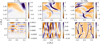 |
Fig. 1 Relative density Δρ (as defined in the text) at t = 2t0, t = 5t0 and t = 10t0 for the O4 model (top) and the WR model (bottom). Here, t0 refers to the models’ respective dynamical timescales of t0 ≈ 5275 s for the O4 model and t0 ≈ 824 s for the WR model. The colorbars do not necessarily have the same range. |
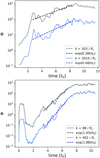 |
Fig. 2 Density power evolution over time of the different wavenumber modes in the O4 model (top) and the WR model (bottom). The blue curves show the evolution of the large-wavenumber mode and the gray curves show the small-wavenumber mode. The dashed curves show the respective exponential fits. |
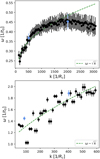 |
Fig. 3 Growth rates calculated from the exponential fit of the density power evolution for multiple wavenumbers in the O4 model (top) and WR model (bottom). The blue dots correspond to the wavenumbers shown in Fig. 2. The errorbars on the growth rates are one standard deviation errors from the nonlinear least squares fitting. The green dashed line is a fit of ω(k). |
4 Analysis
Using Eqs. (30) and (32), we can predict the unstable regions for the convective mode and the strange mode for both models. Moreover, the imaginary parts ωI of the resulting frequencies in Eqs. (26) and (31) for these modes allow us to estimate the growth rates set by both instabilities. Eqs. (26) and (31) depend on the direction of the wave vector so whenever we calculate characteristic values for the growth rates, we assume that the wave vector makes a 45° angle with the vertical direction.
4.1 O stars
In the top panel of Fig. 4, we show the laterally averaged density structure for the snapshot at t = 2t0 of the O4 model, which corresponds to the time where we started the exponential fit in the top panel of Fig. 2. With the red and blue dashed lines, we show the edges of the regions where the convective mode and the strange mode become unstable or overstable, respectively. We note that there is some overlap between the convective region and the strange mode region. However, the convective region is located completely below the photosphere while the strange mode region starts closer to the photosphere and extends into the wind. It must be noted that these regions are predicted using analytic results that are derived in the optically thick limit which means that these criteria can really only be applied in the subsurface layers. Therefore, we focus solely on the sub-surface region, dominated by the convective instability in the O4 model, albeit with a smaller strange mode region also. The growth rates we calculate from Eqs. (26) and (31) depend on the local background variables at every grid point, but as a characteristic value, we can take the mean value over all grid points in the same region where we computed the power evolution (Fig. 2) in the previous section, namely from ɀ = 1.1 Rc to ɀ = 1.3Rc and y = −0.1 Rc to y = 0.1 Rc. For k ≈ 503/Rc, the small wavenumber mode in the top panel of Fig. 2, this results in a mean convective growth rate of 〈ωg〉 ≈ 0.0014/t0. The growth rate for the strange mode can also be computed, calculating the opacity gradient in Eq. (31) directly from the opacity table used in the model. The growth rate of the strange mode in the O4 model, which is independent of k, is calculated to be 〈ωac〉 ≈ −0.37/t0. Thus, the strange modes are, on average, damped in the region where the power spectra are computed. The convective growth rate, on the other hand, is on average positive but the average value is two orders of magnitude smaller than the result for the small-wavenumber mode in Fig. 2. Since the theoretical convective growth rate does not agree with the computed growth rates and since the k-dependence in the top panel of Fig. 3 does not show the characteristic ~1/k2 scaling, the convective instability is unlikely to be the origin of structure formation in the O4 model. While the plateau in the top panel of Fig. 3 could be in line with the ~k0 scaling of the strange mode instability, these strange modes are expected to be damped in the studied region and therefore, the strange mode instability also seems to be an unlikely explanation.
4.2 Wolf–Rayet stars
In the bottom panel of Fig. 4, we show the average density structure at t = 2t0 for the WR model, where we once again indicate the region in which the convective mode could be unstable according to Eq. (30) by the red dashed lines. The convective region is located deeper below the photosphere as compared to the results for the O4 model and it also seems to extend further. The key difference with the previous O4 model is the strange mode region. Whereas in the O4 model, the strange mode instability region is clearly bounded and located close to the photosphere, this mode is predicted to be overstable over the entire radial extent of the WR model, extending far down to the lower boundary. Due to the initial conditions of the WR model being less smooth than those of the O4 model, the theoretical growth rates fluctuate heavily within the convective region, even going negative at multiple vertical points. Therefore, the estimated mean convective growth rate for k = 88/Rc over the range from ɀ = 1.3Rc to ɀ = 1.8Rc and y = −0.25Rc to y = 0.25Rc (consistent with the slice that was used to produce the bottom panel in Fig. 2) still comes out slightly damped with 〈ωg〉 ≈ −0.0050/t0. The mean growth rate for the strange mode in this same region is 〈ωac〉 ≈ 1.53/t0. The strange mode growth rate matches the order of magnitude of the computed growth rates in the bottom panel of Fig. 3 quite well, especially on the small-wavenumber end. However, the k-dependence in the bottom panel of Fig. 3 also does not match the characteristic ~ 1 /k2 or ~k0 behavior of either instability. As both the theoretical value of the convective growth rate as well as the k-dependence does not match the results of the WR model, the convective instability can most likely be excluded as a potential structure formation mechanism. For the strange modes, however, the result is less clear as the theoretical strange mode growth rate does match the computed growth rates quite well, but the k-dependence is different. Although, it must be noted that the theoretical k-dependence turns out to be different in the limit of fully negligible gas pressure, see Section 5.1 for further discussion.
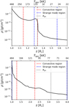 |
Fig. 4 Average density profiles at t = 2t0 for the O4 model (top) and the WR model (bottom), with the vertical axis in logarithmic scale. The red dashed lines indicate the predicted convective region and the blue dashed lines indicate the predicted strange mode region. In the WR model, the whole domain is predicted to be unstable to strange modes, which we indicate by the blue dashed lines at the edges of the plot. The dotted black lines indicate the photosphere. |
4.3 Comparison
The differences in theoretical growth rates and instability regions between the O4 model and the WR model can be explained by analyzing Eqs. (29) and (35), as done in Section 2.3, and giving some characteristic numbers at the peak of the iron bump in the respective models.
For the convective mode, the growth rate is determined by the ratio of the diffusion timescale and the total Brunt–Väisälä frequency. For k = 100/R⊙, which corresponds to kWR = 100/Rc and kO = 1350/Rc, we find that tdiff,O ≈ 0.192 s and tdiff,WR ≈ 0.013 s so the diffusion time in the O4 model is a factor fourteen larger than the diffusion time in the WR model. This difference can be explained by referring back to our earlier rewriting of tdiff = τλtff. As the wavenumber (and hence the wavelength) is the same, tff does not change between the two models, so the difference in diffusion time comes entirely from the factor τλ. This difference in optical depth comes mainly from the larger density in the iron bump region of the O4 model. Thus, due to the larger optical depth, the O4 model experiences less damping by radiative diffusion. The total Brunt–Väisälä frequency depends on gradients of density and (gas or radiation) pressure. The density inversion in the initial conditions of the O4 model makes the second term in Eq. (23) absolutely positive, which means that  is always true. Thus, the density inversion that arises from trying to maintain hydrostatic equilibrium when Γ > 1 is inherently unstable to convection in luminous stellar envelopes (Langer 1997). Since the WR star is able to launch a wind from the iron bump, there is no density inversion and therefore not necessarily an instability. This, together with the quick radiative diffusion, makes the convective instability less prominent in the WR stars.
Another major difference between the O4 model and the WR model is the strange mode growth rates and instability region. This comes from the interplay between the different terms in Eq. (35). The boundaries of the instability region are determined by the competition between Θρ and Dr. Interestingly, we find that Θρ is on the same order in the O4 model and the WR model with Θρ ≈ 0.15. Therefore, the difference between the two models comes entirely from the radiative drag term. We find that Dr in the O4 model is around a factor of seventy larger than in the WR model. The main difference in this radiation drag term comes from the flux factor in the definition of Dr , since the flux of the WR model is indeed larger than the flux in the O4 model. We can also relate this to the local flux temperature  that we defined previously. This
  is indeed larger in WR stars than in O stars and this explains why WR stars experience less radiative drag. Due to the smaller radiative drag, we expect the strange modes to be more prominent in the WR model than in the O4 model.
5 Discussion
5.1 Growth rate k-dependence
As discussed above, the top panel of Fig. 3 shows that the growth rates of both the O4 model and the WR model have a very peculiar k-dependence in the sense that they do not match either instability studied in Section 2.3. Therefore, we attempt to give suggestions for alternative formation mechanisms.
An instability that has not been discussed here is the Rayleigh-Taylor (RT) instability which arises when a higher density gas overlays a lower density gas. However, the density inversion in Fig. 4 is inherently unstable to this instability as well. Furthermore, although the WR model does not show any density inversions on average, some outflowing density inversions may appear in the early stages of the simulation (see Fig. 3 in Moens et al. 2022b). Therefore, both the O4 model and the WR model could in principle experience RT-like instabilities, although we expect a larger effect in the O4 model due to the density inversion being quite prominent. Such a RT-like instability does not appear in the stability analysis in Section 2.3 because we assumed the background state to be locally uniform. To find these RT instabilities, we should have considered a background state with a density jump at an interface with certain boundary conditions (Jacquet & Krumholz 2011). This could, in principle, be done but this is outside the scope of the current work. Jacquet & Krumholz (2011) studied the linear growth of radiative RT instabilities in both the optically thin and the optically thick limit. Furthermore, in the appendix of Jiang et al. (2013), radiative RT instabilities in the limit of negligible absorption opacity were studied. In all of these different limits, the same  scaling of the classical RT instability was found. Thus, although it is not entirely clear which limits can be safely applied to the simulations studied here, radiative RT instabilities generally seem to lead to the same k-dependence as found in our simulations.
Another possibility is the strange mode instability result in the negligible gas pressure limit found in Blaes & Socrates (2003), their section 3.3, in which they neglected gas pressure altogether and found
 (39)
(39)
This result also reproduces this  dependence. It could be argued that this limit applies to these systems, as they are radiation-pressure dominated, although the gas pressure still accounts for up to 30% of the total pressure at the density inversion in the O4 model. In the WR model, however, on average only about 0.5% of the total pressure is accounted for by the gas pressure. Thus, at least for the O4 model, it is unclear whether this limit can be applied.
Therefore, both RT-like instabilities and strange mode instabilities in the limit of negligible gas pressure would produce the same scaling we find in our simulations. However, since these instabilities have the same k-dependence, it is difficult to distinguish between them and we have also not formally derived these scalings for our problem set-up. The task of conclusively identifying which instability is leading to this  scaling is left for future work.
5.2 Observational implications
Atmospheric micro and macroturbulence. The turbulence generated in the envelopes and atmospheres of massive stars can lead to multiple observational effects. One noteworthy effect is the relation between turbulent motions and the so-called microturbulence or macroturbulence, additional ad-hoc velocity broadening terms that were introduced to explain excessive line broadening that could not be explained by rotational or thermal broadening (Conti & Ebbets 1977; Gray 2008; Simón-Díaz et al. 2017). It has been suggested that the turbulent sub-surface layer associated with the iron bump can excite gravity waves which lead to velocity fluctuations at the surface and can therefore possibly be related to microturbulence (Cantiello et al. 2009). Moreover, supersonic turbulence up to the surface, as seen in simulations like those presented here, is a natural explanation for the inferred macroturbulent velocities (Jiang et al. 2015; Schultz et al. 2022; Debnath et al. 2024). On the other hand, gravity waves excited by core-convection or this sub-surface turbulent zone and traveling up to the stellar surface have also been discussed with respect to the origin of such macroturbulence (Aerts et al. 2009; Simón-Díaz et al. 2017; Serebriakova et al. 2024). The origin of these structures is important in the context of macroturbulence as the driving mechanism of the turbulent structures impacts both their final velocities and their distributions. For example, gravity waves are excited preferentially in the lateral directions, which may lead to turbulent velocity profiles dominated by the tangential component. However, such laterally dominated distributions are not necessarily the outcome for the excitation mechanisms suggested in Section 5.1. Since different velocity distributions give rise to different shapes of the line profile broadening functions (see overview in Gray 2008), detailed high-resolution spectroscopy may be able to distinguish between these different scenarios.
Leakage of light. As mentioned above, the origin of the structures also has an impact on their final shapes which may affect the porosity properties of the turbulent atmosphere. Such porosity generally refers to the additional light leakage that can occur from an inhomogeneous gaseous system as compared to a homogeneous one of the same mass, and is important in a wide range of astrophysical environments. In the context of stellar winds of massive stars, such a porous atmosphere can lead to reduced mass loss rates for the same total luminosity (Shaviv 2000). The quantitative amount of light-leakage can depend on the shapes of the structures. For example, finger-like, radially extended structures such as those seen in this paper may lead to larger escape fractions for photons emitted in the radial direction than in the lateral. As one specific example, this might have a pronounced effect on the number of continuum photons emitted from the deeper photosphere which are able to interact with resonant lines in the wind. Due to Doppler shifts, these interactions can only occur on surfaces of constant line-of-sight velocities and hence such “velocity–porosity” effects (Oskinova et al. 2007; Sundqvist et al. 2010; Owocki 2014) have been shown to be particularly important for line formation in massive-star winds (Prinja & Massa 2013; Šurlan et al. 2012; Hawcroft et al. 2021; Brands et al. 2022). Current implementations of velocityporosity into standard spectroscopic analysis tools (Sundqvist & Puls 2018), however, assume isotropic effects. In view of the results found here, it is thus not clear to what extent the amount of line photon leakage through the atmosphere is properly captured within current spectroscopic studies of massive stars.
5.3 On the nature of sub-surface turbulent zones in massive stars
It has long been known that stellar envelopes approaching the Eddington limit will trigger a sub-surface convection zone (Langer 1997; Maeder 2009). Due to the iron bump pushing part of the stellar envelope to the Eddington limit, the sub-surface convection zone that is created is often linked to the near-surface turbulence in massive stars. Our results, however, suggest that convection is actually not the main formation mechanism of the envelope and atmospheric turbulence in O stars and WR stars.
It is important to note, though, that the initial conditions of the presented simulations may have an impact on the formation of structures. Especially for the O4 model, the initial conditions assume a hydrostatic envelope in radiative equilibrium, resulting in a density inversion. The final average structure of the non-linear simulations, however, no longer shows such a density inversion. Furthermore, the average structure also involves significant turbulent pressure support. Therefore, the average structure deviates quite heavily from the initial conditions, meaning that the relaxation of the initial conditions is significant in these simulations. Further work is needed to study exactly how sensitive the structure formation is to the initial conditions. Nevertheless, with this in mind, our results here can still be used to gain further insights into the underlying physics of the formation of envelope turbulence in massive stars.
We find that, at least in the case of O stars and WR stars, while the convective instability is indeed expected to be present in the iron bump region, the initial structure formation does not show the 1/k2 dependence expected for radiative convection. This indicates that other instabilities, such as potentially the strange mode instability and RT-like instabilities, could be the dominant driving force behind this turbulence. Additionally, analysis of the final, non-linear turbulent states in simulations of O stars and WR stars shows that energy transport by enthalpy (or, convection) is very inefficient in these atmospheres, with ≳90% of the total energy being carried by diffuse radiation even at the peak of the iron bump (Jiang et al. 2015; Debnath et al. 2024). By contrast, the atmospheric turbulent pressure support is very significant, that is, reaching similar levels as radiation pressure in the photospheric layers of the O4 model. Therefore, in view of our results, the treatment of this turbulent zone as a classical convection zone in 1D stellar structure and evolution models should be revisited.
Interestingly, a similar deviation from a ω ~ 1/k2 dependence is found in the StarTop model in Jiang et al. (2015). This is the model whose parameters most closely resemble the parameters of the O4 model. Similar to our O4 model, their StarTop model is in the regime where convection is an inefficient mode of energy transport. By contrast, in their model StarDeep, which lies in the efficient convection regime, they do approximately reproduce the ~1/k2 dependence. This suggests that the convective instability might become more significant as enthalpy becomes more efficient in transporting energy. We notice a potential anti-correlation between such convective energy transport and the strength of the strange mode instability. Namely, efficiency of energy transport through convection scales as ~ciE/Fdiff (Gräfener et al. 2012; Jiang et al. 2015; Debnath et al. 2024), but this is precisely the damping term Dr (in the radiation-pressure dominated limit) that competes against the opacity driving term Θρ in the strange mode instability. Thus, in regimes of efficient convective energy transport, the strange mode instability is expected to also be strongly damped (or even non-existent). Thus, it might be that the structure formation mechanism and the turbulent properties systematically change as one moves to different stellar regimes with varying Teff (see also Schultz et al. 2023).
6 Summary and outlook
The turbulent sub-surface layers of O stars and WR stars play an important role both for the stellar structure as well as for the emergent spectra. However, the origin of this turbulence, albeit often linked to a sub-surface convection zone triggered by the iron bump, has not been extensively studied. In this paper, we studied the formation mechanism of the emergent turbulence in multi-D simulations of WR stars and O stars by Moens et al. (2022b) and Debnath et al. (2024), respectively. Based on work by Blaes & Socrates (2003), we identified multiple instabilities that could operate in the optically thick, radiation-pressure dominated envelopes of these stars. Two possible instabilities are found: the convective instability and a local variant of the strange mode instability. Studying the analytical growth rates of these instabilities shows that the convective growth rate depends on wavenumber k as ωg ~ 1/k2 and the strange mode is independent of wavenumber, that is, ωac ~ k0. The growth rates of the structures in the simulations were deduced by computing power spectra of the relative density, tracking the power evolution over time and fitting an exponential to the results. We find that  for both the O4 model and the WR model. Therefore, the k-dependence from the simulations is incompatible with either instability studied here. Instead, this
  scaling could potentially be compatible with the Rayleigh-Taylor instability (Jacquet & Krumholz 2011; Jiang et al. 2013) or the strange mode instability in the limit of negligible gas pressure (Blaes & Socrates 2003). In any case, we clearly find that the structure formation in both models does not agree with the classical radiatively modified convection picture as we do not reproduce the expected ω ~ 1/k2 scaling. This is a significant result since, as previously mentioned, this sub-surface turbulent layer is often treated as a sub-surface convective layer (for instance, in stellar evolution codes such as MESA; Paxton et al. 2013) in the sense that energy transport is often assumed to be efficient, which is not the case for the simulations analyzed here. Moreover, the different formation mechanism impacts the final shape and size of the structures.
As the exact structure formation mechanism in these simulations remains inconclusive for now, future work will attempt to identify other instabilities by modifying the stability analysis accordingly. Another direct follow-up to this work would be to quantify the properties of the emergent non-linear turbulent structures. In particular, we would like to quantify the energy distribution in the turbulent medium by computing energy power spectra and then comparing this to classical turbulence theory (see for example Schmidt et al. 2009). It would also be useful to quantify the characteristic length scale of these structures and distinguish between the lateral and vertical components.
Furthermore, we wish to extend this analysis to different stellar regimes such as Luminous Blue Variables or Red Supergiants. As discussed in the previous section, we expect to find differences between our results here and those regimes where convective energy transport is supposed to be more efficient.
Acknowledgements
The computational resources used for this work were provided by Vlaams Supercomputer Centrum (VSC) funded by the Research Foundation-Flanders (FWO) and the Flemish Government. CVdS, JOS, DD and NM acknowledge the support of the European Research Council (ERC) Horizon Europe under grant agreement number 101044048. JOS further acknowledges the support of the Belgian Research Foundation Flanders (FWO) Odysseus program under grant number G0H9218N, and from FWO grant G077822N. The authors thank the referee Dr. Achim Feldmeier for constructive criticism on the manuscript. The authors would like to thank all members of the KUL-EQUATION group for fruitful discussion, comments, and suggestions. The following packages were used to analyze the data: NumPy (Harris et al. 2020), SciPy (Virtanen et al. 2020), matplotlib (Hunter 2007), Python amrvac_reader (Keppens et al. 2021).
Appendix A Additional considerations for a mean background outflow
A.1 Advection timescale
As previously mentioned, WR stars can launch an optically thick wind from the sub-surface layers whereas an O star has a fully optically thin wind, initiated outside the photosphere, on top of a turbulent deeper atmosphere. For WR stars, the average sonic point can therefore lie within the iron bump region, meaning that there might already be a significant outflow in the structure formation region. This leads to a competing timescale: any structures that grow due to an instability must be able to grow to non-linear scales before the wind expels a significant amount of mass from the unstable region. This same reasoning was already put forward in Cantiello et al. (2009) for the helium opacity bump, which is located even closer to the photosphere. As in Cantiello et al. (2009), we may define a certain mass loss timescale for our WR model as the time tṀ it takes for the wind to expel an amount of mass equal to the mass in the unstable region, namely
 (A.1)
(A.1)
where ∆M is the total mass contained within the unstable region and Ṁ is the mass loss rate. We focus on the convective region indicated in Fig. 4 which extends over ∆ɀ ≈ 1.3Rc. We calculate a characteristic ∆M = 4πɀ2∆ɀ〈ρ〉 = 1.94 × 10⁻⁹ M⊙ in a spherical shell at a distance ɀ, where we have taken the ɀ- coordinate at the midpoint of the convective region so ɀ = 1.95Rc and 〈ρ〉 = 1.9 × 10⁻¹⁰ g/cm3 is the laterally averaged density at this midpoint. The typical mass loss rate in this convective region can be calculated as the mass loss rate at the midpoint Ṁ = 4πɀ2〈υɀρ〉 = 6.5 × 10⁻⁵ M⊙/yr. Using these estimates, we find
 (A.2)
(A.2)
This time is equivalent to the typical advection time of a fluid parcel across the convective region. This time needs to be compared to the typical time it takes for convection to develop. We can estimate the minimal time that is needed for a perturbation to grow due to the convective instability. The maximum growth rate in the convective region of the WR stars is ωg = 0.34/t0 so the minimal time that is needed for a perturbation to grow by a factor of e is t = 1/ωg ≈ 2400 s. This time is already larger than tṀ and it is important to note that this estimate is the minimal convective growth time, which is only valid at a specific point in the convective region, but not everywhere. Thus, on average, it takes much longer for convection to develop which means that the mass loss time tṀ is significantly smaller than this growth time. Therefore, the convective region is completely cleared of material before convection can fully develop.
The case for the strange modes is different. Firstly, the instability region is larger than the convective region. Considering only the sub-photospheric layers, the extent of the instability region is now ∆ɀ ≈ 2.2Rc which results in ∆M = 3.3 × 10⁻⁹M⊙ and Ṁ = 6.5 × 10⁻⁵M⊙/yr. Therefore, the advection time becomes
 (A.3)
(A.3)
The maximum acoustic growth rate in the sub-surface region is ω ≈ 1.91/t0 which results in a minimal growth time t ≈ 430 s. Thus, the growth time is now significantly shorter than the advection time. Furthermore, these strange modes are propagating waves as opposed to the gravity waves. Hence, the strange mode instability is a traveling instability instead of an instability at a fixed vertical position. Therefore, the strange modes will not be impacted by material being cleared out of a certain fixed region as they will propagate out of this region also. For these reasons, we do not expect the growth of the strange modes to be substantially impacted by the sub-surface outflow.
A.2 Eulerian vs Lagrangian frame
As explained in Section 2.3, the resulting dispersion relation from the linear stability analysis is obtained by assuming perturbations on top of a certain background equilibrium state. This equilibrium state was taken to be static, but this approximation is questionable for the WR stars, in particular, as the velocities in the region of interest are already significant. For the O stars, this approximation seems reasonable since the average velocity in the sub-surface layers is close to zero. The power spectra in Section 3 were computed by taking a cut of the grid at a fixed location (see Section 3), that is, by studying the structures in an Eulerian reference frame. However, in reality, the result for the dispersion relation in Section 2.3 is only valid in a reference frame moving with the local fluid velocity, that is, a Lagrangian frame. This means that the cut of the grid should actually follow the local fluid velocity. Implementing this in practice is nontrivial since the gas is accelerating so the top part of the cut will have a larger average gas velocity than the bottom part in which case the size of the cut would not be conserved. To simplify, we started with a cut of 0.5Rc × 0.5Rc, as before, and at each time step, we calculated the total average radial gas velocity υavg within this cut. Then, for the next time step, we moved the cut by a vertical distance υavg∆t. For each time step, the power in a certain mode was calculated using the procedure outlined in Section 3. To avoid complications with the different refinement levels as the cut moves through the box, we re-ran the WR simulation on a full grid at the base refinement of 1024 × 128 cells. In this method, the initial position of the cut is a free parameter. The only restriction we want to impose is that the cut moves through the full iron bump region, meaning that the initial location of the lower boundary of the cut should be below the iron bump. Therefore, we sampled four different initial lower boundary positions, namely at ɀ = 1.1 Rc, ɀ = 1.2Rc, ɀ = 1.3Rc and ɀ = 1.4Rc to study how this initial position might affect the final curves. Inspection of the results shows that the initial position does affect the computed growth rates and we believe this is due to the time-dependent nature of these simulations, meaning that not all regions are always equally structured and by changing the initial position, we track more or less structured regions with different behavior. As such, we took an average of the four different starting positions in order to obtain a more general view of the power evolution obtained from this Lagrangian method. In Fig. A.1, this average Lagrangian power evolution is shown as the blue curve and the black curve shows the evolution curve in the Eulerian frame as used above. From this figure, it is clear that in an average sense, the power evolution is qualitatively the same between the Lagrangian method and the Eulerian method. As a further comparison, we show the average growth rates from this Lagrangian frame analysis as a function of wavenumber in Fig. A.2. The average was computed as a weighted average of the results from thirty different starting positions, ranging from ɀ = 1.1 Rc to ɀ = 1.4Rc in steps of ∆ɀ = 0.01 Rc. This figure shows that the general k-dependence agrees well between the Eulerian and the Lagrangian analysis. Repeating the previous analysis using the Lagrangian method comes with some complications. Firstly, as already mentioned, the results are quite sensitive to the starting position. Secondly, as we are only interested in the optically thick envelope, the analysis can only be done as long as the cut stays below the photosphere. Because of this, we can only track the power evolution for shorter periods of time. Due to these reasons, and because the two methods seem to give qualitatively similar results, the Eulerian analysis is favored in this work.
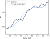 |
Fig. A.1 Power evolution comparison between the Eulerian frame and the Lagrangian frame. The black curve shows the power evolution in the usual Eulerian frame and the blue curve shows the power evolution for the average Lagrangian frame, where the averaging was done for four different starting positions (see text). |
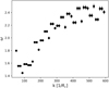 |
Fig. A.2 Average growth rates for multiple wavenumbers from the Lagrangian frame analysis. The final growth rate for a certain wavenumber is a weighted average of thirty growth rates from different starting positions between ɀ = 1.1 Rc and ɀ = 1.4Rc in steps of ∆ɀ = 0.01 Rc. |
References
- Aerts, C., Puls, J., Godart, M., & Dupret, M.-A. 2009, A&A, 508, 409 [NASA ADS] [CrossRef] [EDP Sciences] [Google Scholar]
- Blaes, O., & Socrates, A. 2003, ApJ, 596, 509 [CrossRef] [Google Scholar]
- Brands, S. A., de Koter, A., Bestenlehner, J. M., et al. 2022, A&A, 663, A36 [Google Scholar]
- Cantiello, M., Langer, N., Brott, I., et al. 2009, A&A, 499, 279 [NASA ADS] [CrossRef] [EDP Sciences] [Google Scholar]
- Castor, J. I., Abbott, D. C., & Klein, R. I. 1975, ApJ, 195, 157 [Google Scholar]
- Conti, P. S., & Ebbets, D. 1977, ApJ, 213, 438 [CrossRef] [Google Scholar]
- Crowther, P. A. 2007, ARA&A, 45, 177 [Google Scholar]
- Debnath, D., Sundqvist, J. O., Moens, N., et al. 2024, A&A, 684, A177 [NASA ADS] [CrossRef] [EDP Sciences] [Google Scholar]
- Dessart, L., & Owocki, S. P. 2002, A&A, 393, 991 [NASA ADS] [CrossRef] [EDP Sciences] [Google Scholar]
- Eversberg, T., Lépine, S., & Moffat, A. F. J. 1998, ApJ, 494, 799 [NASA ADS] [CrossRef] [Google Scholar]
- Gautschy, A., & Glatzel, W. 1990, MNRAS, 245, 597 [NASA ADS] [Google Scholar]
- Glatzel, W. 1994, MNRAS, 271, 66 [NASA ADS] [CrossRef] [Google Scholar]
- González-Torà, G., Sander, A. A. C., Sundqvist, J. O., et al. 2024, A&A, submitted [arXiv:2501.14511] [Google Scholar]
- Gräfener, G., Koesterke, L., & Hamann, W. R. 2002, A&A, 387, 244 [NASA ADS] [CrossRef] [EDP Sciences] [Google Scholar]
- Gräfener, G., Owocki, S. P., & Vink, J. S. 2012, A&A, 538, A40 [NASA ADS] [CrossRef] [EDP Sciences] [Google Scholar]
- Gray, D. F. 2008, The Observation and Analysis of Stellar Photospheres (Cambridge, UK: Cambridge University Press) [Google Scholar]
- Hamann, W. R., & Gräfener, G. 2004, A&A, 427, 697 [NASA ADS] [CrossRef] [EDP Sciences] [Google Scholar]
- Harris, C. R., Millman, K. J., van der Walt, S. J., et al. 2020, Nature, 585, 357 [NASA ADS] [CrossRef] [Google Scholar]
- Hawcroft, C., Sana, H., Mahy, L., et al. 2021, A&A, 655, A67 [NASA ADS] [CrossRef] [EDP Sciences] [Google Scholar]
- Hillier, D. J., & Lanz, T. 2001, in Astronomical Society of the Pacific Conference Series, 247, Spectroscopic Challenges of Photoionized Plasmas, eds. G. Ferland & D. W. Savin, 343 [NASA ADS] [Google Scholar]
- Hillier, D. J., & Miller, D. L. 1998, ApJ, 496, 407 [NASA ADS] [CrossRef] [Google Scholar]
- Howarth, I. D., Siebert, K. W., Hussain, G. A. J., & Prinja, R. K. 1997, MNRAS, 284, 265 [NASA ADS] [CrossRef] [Google Scholar]
- Hunter, J. D. 2007, Comput. Sci. Eng., 9, 90 [NASA ADS] [CrossRef] [Google Scholar]
- Iglesias, C. A., & Rogers, F. J. 1996, ApJ, 464, 943 [NASA ADS] [CrossRef] [Google Scholar]
- Jacquet, E., & Krumholz, M. R. 2011, ApJ, 730, 116 [NASA ADS] [CrossRef] [Google Scholar]
- Jiang, Y.-F., Davis, S. W., & Stone, J. M. 2013, ApJ, 763, 102 [NASA ADS] [CrossRef] [Google Scholar]
- Jiang, Y.-F., Cantiello, M., Bildsten, L., Quataert, E., & Blaes, O. 2015, ApJ, 813, 74 [Google Scholar]
- Keppens, R., Teunissen, J., Xia, C., & Porth, O. 2021, Comput. Math. Appl., 81, 316 [Google Scholar]
- Keppens, R., Popescu Braileanu, B., Zhou, Y., et al. 2023, A&A, 673, A66 [NASA ADS] [CrossRef] [EDP Sciences] [Google Scholar]
- Langer, N. 1997, in Luminous Blue Variables: Massive Stars in Transition, 120, 83 [NASA ADS] [Google Scholar]
- Lepine, S. 1994, Ap&SS, 221, 371 [NASA ADS] [CrossRef] [Google Scholar]
- Levermore, C. D., & Pomraning, G. C. 1981, ApJ, 248, 321 [NASA ADS] [CrossRef] [Google Scholar]
- Maeder, A. 2009, Physics, Formation and Evolution of Rotating Stars, Astronomy and Astrophysics Library (Berlin, Heidelberg: Springer Berlin Heidelberg) [CrossRef] [Google Scholar]
- Michaux, Y. J. L., Moffat, A. F. J., Chené, A.-N., & St-Louis, N. 2014, MNRAS, 440, 2 [NASA ADS] [CrossRef] [Google Scholar]
- Moens, N., Sundqvist, J. O., El Mellah, I., et al. 2022a, A&A, 657, A81 [NASA ADS] [CrossRef] [EDP Sciences] [Google Scholar]
- Moens, N., Poniatowski, L. G., Hennicker, L., et al. 2022b, A&A, 665, A42 [NASA ADS] [CrossRef] [EDP Sciences] [Google Scholar]
- Moffat, A. F. J., Drissen, L., Lamontagne, R., & Robert, C. 1988, ApJ, 334, 1038 [NASA ADS] [CrossRef] [Google Scholar]
- Oskinova, L., Hamann, W.-R., & Feldmeier, A. 2007, A&A, 476, 1331 [NASA ADS] [CrossRef] [EDP Sciences] [Google Scholar]
- Owocki, S. P. 2014, Instabilities in the Envelopes and Winds of Very Massive Stars (Springer International Publishing), 113 [Google Scholar]
- Owocki, S. P., & Puls, J. 1996, ApJ, 462, 894 [Google Scholar]
- Owocki, S. P., & Rybicki, G. B. 1984, ApJ, 284, 337 [Google Scholar]
- Owocki, S. P., & Rybicki, G. B. 1985, ApJ, 299, 265 [NASA ADS] [CrossRef] [Google Scholar]
- Owocki, S. P., & Rybicki, G. B. 1991, ApJ, 368, 261 [NASA ADS] [CrossRef] [Google Scholar]
- Paxton, B., Cantiello, M., Arras, P., et al. 2013, ApJS, 208, 4 [Google Scholar]
- Poniatowski, L. G., Sundqvist, J. O., Kee, N. D., et al. 2021, A&A, 647, A151 [NASA ADS] [CrossRef] [EDP Sciences] [Google Scholar]
- Prinja, R., & Massa, D. 2013, A&A, 559, A15 [NASA ADS] [CrossRef] [EDP Sciences] [Google Scholar]
- Puls, J., Urbaneja, M. A., Venero, R., et al. 2005, A&A, 435, 669 [NASA ADS] [CrossRef] [EDP Sciences] [Google Scholar]
- Puls, J., Markova, N., Scuderi, S., et al. 2006, A&A, 454, 625 [NASA ADS] [CrossRef] [EDP Sciences] [Google Scholar]
- Puls, J., Najarro, F., Sundqvist, J. O., & Sen, K. 2020, A&A, 642, A172 [EDP Sciences] [Google Scholar]
- Rubio-Díez, M. M., Sundqvist, J. O., Najarro, F., et al. 2022, A&A, 658, A61 [NASA ADS] [CrossRef] [EDP Sciences] [Google Scholar]
- Rybicki, G. B., Owocki, S. P., & Castor, J. I. 1990, ApJ, 349, 274 [NASA ADS] [CrossRef] [Google Scholar]
- Saio, H., Baker, N. H., & Gautschy, A. 1998, MNRAS, 294, 622 [NASA ADS] [CrossRef] [Google Scholar]
- Sander, A., Hamann, W. R., & Todt, H. 2012, A&A, 540, A144 [NASA ADS] [CrossRef] [EDP Sciences] [Google Scholar]
- Santolaya-Rey, A. E., Puls, J., & Herrero, A. 1997, A&A, 323, 488 [NASA ADS] [Google Scholar]
- Schmidt, W., Federrath, C., Hupp, M., Kern, S., & Niemeyer, J. C. 2009, A&A, 494, 127 [NASA ADS] [CrossRef] [EDP Sciences] [Google Scholar]
- Schultz, W. C., Bildsten, L., & Jiang, Y.-F. 2022, ApJ, 924, L11 [NASA ADS] [CrossRef] [Google Scholar]
- Schultz, W. C., Bildsten, L., & Jiang, Y.-F. 2023, ApJ, 951, L42 [NASA ADS] [CrossRef] [Google Scholar]
- Serebriakova, N., Tkachenko, A., & Aerts, C. 2024, A&A, 692, A245 [NASA ADS] [CrossRef] [EDP Sciences] [Google Scholar]
- Shaviv, N. J. 2000, ApJ, 532, L137 [NASA ADS] [CrossRef] [Google Scholar]
- Shaviv, N. J. 2001, ApJ, 549, 1093 [NASA ADS] [CrossRef] [Google Scholar]
- Simón-Díaz, S., Godart, M., Castro, N., et al. 2017, A&A, 597, A22 [CrossRef] [EDP Sciences] [Google Scholar]
- Sundqvist, J., & Puls, J. 2018, A&A, 619, A59 [NASA ADS] [CrossRef] [EDP Sciences] [Google Scholar]
- Sundqvist, J., Puls, J., & Feldmeier, A. 2010, A&A, 510, A11 [NASA ADS] [CrossRef] [EDP Sciences] [Google Scholar]
- Sundqvist, J. O., Owocki, S. P., & Puls, J. 2018, A&A, 611, A17 [NASA ADS] [CrossRef] [EDP Sciences] [Google Scholar]
- Šurlan, B., Hamann, W.-R., Kubát, J., Oskinova, L. M., & Feldmeier, A. 2012, A&A, 541, A37 [NASA ADS] [CrossRef] [EDP Sciences] [Google Scholar]
- Virtanen, P., Gommers, R., Oliphant, T. E., et al. 2020, Nature Methods, 17, 261 [CrossRef] [Google Scholar]
- Xia, C., Teunissen, J., El Mellah, I., Chané, E., & Keppens, R. 2018, ApJS, 234, 30 [Google Scholar]
All Tables
All Figures
|
Fig. 1 Relative density Δρ (as defined in the text) at t = 2t0, t = 5t0 and t = 10t0 for the O4 model (top) and the WR model (bottom). Here, t0 refers to the models’ respective dynamical timescales of t0 ≈ 5275 s for the O4 model and t0 ≈ 824 s for the WR model. The colorbars do not necessarily have the same range. |
| In the text | |
|
Fig. 2 Density power evolution over time of the different wavenumber modes in the O4 model (top) and the WR model (bottom). The blue curves show the evolution of the large-wavenumber mode and the gray curves show the small-wavenumber mode. The dashed curves show the respective exponential fits. |
| In the text | |
|
Fig. 3 Growth rates calculated from the exponential fit of the density power evolution for multiple wavenumbers in the O4 model (top) and WR model (bottom). The blue dots correspond to the wavenumbers shown in Fig. 2. The errorbars on the growth rates are one standard deviation errors from the nonlinear least squares fitting. The green dashed line is a fit of ω(k). |
| In the text | |
|
Fig. 4 Average density profiles at t = 2t0 for the O4 model (top) and the WR model (bottom), with the vertical axis in logarithmic scale. The red dashed lines indicate the predicted convective region and the blue dashed lines indicate the predicted strange mode region. In the WR model, the whole domain is predicted to be unstable to strange modes, which we indicate by the blue dashed lines at the edges of the plot. The dotted black lines indicate the photosphere. |
| In the text | |
|
Fig. A.1 Power evolution comparison between the Eulerian frame and the Lagrangian frame. The black curve shows the power evolution in the usual Eulerian frame and the blue curve shows the power evolution for the average Lagrangian frame, where the averaging was done for four different starting positions (see text). |
| In the text | |
|
Fig. A.2 Average growth rates for multiple wavenumbers from the Lagrangian frame analysis. The final growth rate for a certain wavenumber is a weighted average of thirty growth rates from different starting positions between ɀ = 1.1 Rc and ɀ = 1.4Rc in steps of ∆ɀ = 0.01 Rc. |
| In the text | |
Current usage metrics show cumulative count of Article Views (full-text article views including HTML views, PDF and ePub downloads, according to the available data) and Abstracts Views on Vision4Press platform.
Data correspond to usage on the plateform after 2015. The current usage metrics is available 48-96 hours after online publication and is updated daily on week days.
Initial download of the metrics may take a while.