| Issue |
A&A
Volume 691, November 2024
|
|
|---|---|---|
| Article Number | A296 | |
| Number of page(s) | 15 | |
| Section | Stellar atmospheres | |
| DOI | https://doi.org/10.1051/0004-6361/202452235 | |
| Published online | 22 November 2024 | |
Abundances of iron-peak elements in 58 bulge spheroid stars from APOGEE
1
Universidade de São Paulo, IAG, Departamento de Astronomia,
05508-090
São Paulo,
Brazil
2
Lund Observatory, Department of Astronomy and Theoretical Physics, Lund University,
Box 43,
221 00
Lund,
Sweden
3
Max Planck Institute for Astronomy,
Königstuhl 17,
69117
Heidelberg,
Germany
4
Instituto de Astronomía, Universidad Católica del Norte,
Av. Angamos 0610,
Antofagasta,
Chile
5
University of Arizona, Steward Observatory,
Tucson,
AZ
85719,
USA
6
Observatório Nacional,
rua General José Cristino 77,
São Cristóvão, Rio de Janeiro
20921-400,
Brazil
7
NSF NOIRLab,
950 N. Cherry Ave.,
Tucson,
AZ
85719,
USA
8
Instituto de Astrofísica de Canarias, C/Via Lactea s/n,
38205
La Laguna, Tenerife,
Spain
9
Departamento de Astrofísica, Universidad de La Laguna,
38206
La Laguna, Tenerife,
Spain
10
Instituto de Astronomía, Universidad Nacional Autónoma de México,
A. P. 106, C.P.
22800,
Ensenada, B. C.,
Mexico
11
Astrophysikalisches Institut Potsdam,
An der Sternwarte 16,
Potsdam
14482,
Germany
12
Universidade Federal do Rio Grande do Sul,
Caixa Postal 15051,
91501-970
Porto Alegre,
Brazil
13
Department of Physics and Astronomy and JINA Center for the Evolution of the Elements (JINA-CEE), University of Notre Dame,
Notre Dame,
IN
46556,
USA
14
Departament de Física Quãntica i Astrofísica (FQA), Universitat de Barcelona (UB),
Martí i Franquès, 1,
08028
Barcelona,
Spain
15
Institut de Ciències del Cosmos, Universitat de Barcelona (IEEC-UB),
Martí i Franquès 1,
08028
Barcelona,
Spain
16
Institut d’Estudis Espacials de Catalunya (IEEC), Edifici RDIT, Campus UPC,
08860
Castelldefels (Barcelona),
Spain
17
Astrophysics Research Institute, Liverpool John Moores University,
Liverpool,
L3 5RF,
UK
18
Instituto de Astrofísica, Facultad de Ciencias Exactas, Universidad Andres Bello,
Fernández Concha 700,
Las Condes, Santiago,
Chile
19
Vatican Observatory,
Vatican City State
00120,
Italy
20
Departamento de Astronomia, Casilla 160-C, Universidad de Concepcion,
Chile
21
Instituto de Investigación Multidisciplinario en Ciencia y Tecnología, Universidad de La Serena. Avenida Raúl Bitrán S/N,
La Serena,
Chile
22
Departamento de Astronomía, Facultad de Ciencias, Universidad de La Serena.
Av. Juan Cisternas 1200,
La Serena,
Chile
23
Universidade Federal de Sergipe, Av. Marechal Rondon, S/N,
49000-000
São Cristóvão,
SE,
Brazil
24
Instituto de Astrofísica, Pontificia Universidad Católica de Chile,
Vicuña Mackenna 4860, Macul, Casilla 306,
Santiago 22,
Chile
25
Université Côte d’Azur, Observatoire de la Côte d’Azur, CNRS, Laboratoire Lagrange,
Nice,
France
26
Centro de Astronomía (CITEVA), Universidad de Antofagasta,
Avenida Angamos 601,
Antofagasta
1270300,
Chile
★ Corresponding author; This email address is being protected from spambots. You need JavaScript enabled to view it.
Received:
13
September
2024
Accepted:
9
October
2024
Abstract
Context. Stars presently identified in the bulge spheroid are probably very old, and their abundances can be interpreted as due to the fast chemical enrichment of the early Galactic bulge. The abundances of the iron-peak elements are important tracers of nucleosynthesis processes, in particular oxygen burning, silicon burning, the weak s-process, and α-rich freeze-out.
Aims. The aim of this work is to derive the abundances of V, Cr, Mn, Co, Ni, and Cu in 58 bulge spheroid stars and to compare them with the results of a previous analysis of data from the Apache Point Observatory Galactic Evolution Experiment (APOGEE).
Methods. We selected the best lines for V, Cr, Mn, Co, Ni, and Cu located within the H-band of the spectrum, identifying the most suitable ones for abundance determination, and discarding severe blends. Using the stellar physical parameters available for our sample from the DR17 release of the APOGEE project, we derived the individual abundances through spectrum synthesis. We then complemented these measurements with similar results from different bulge field and globular cluster stars, in order to define the trends of the individual elements and compare with the results of chemical-evolution models.
Results. We verify that the H-band has useful lines for the derivation of the elements V, Cr, Mn, Co, Ni, and Cu in moderately metalpoor stars. The abundances, plotted together with others from high-resolution spectroscopy of bulge stars, indicate that: V, Cr, and Ni vary in lockstep with Fe; Co tends to vary in lockstep with Fe, but could be showing a slight decrease with decreasing metallicity; and Mn and Cu decrease with decreasing metallicity. These behaviours are well reproduced by chemical-evolution models that adopt literature yields, except for Cu, which appears to drop faster than the models predict for [Fe/H]<−0.8. Finally, abundance indicators combined with kinematical and dynamical criteria appear to show that our 58 sample stars are likely to have originated in situ.
Key words: stars: atmospheres / Galaxy: abundances / Galaxy: bulge
© The Authors 2024
 Open Access article, published by EDP Sciences, under the terms of the Creative Commons Attribution License (https://creativecommons.org/licenses/by/4.0), which permits unrestricted use, distribution, and reproduction in any medium, provided the original work is properly cited.
This article is published in open access under the Subscribe to Open model. This email address is being protected from spambots. You need JavaScript enabled to view it. to support open access publication.
1 Introduction
The very early Galactic bulge formed from a merger of dark matter haloes and their respective matter content, consisting of first-generation stars and globular clusters (GCs) (e.g. Gao et al. 2010). The subsequent processes of bulge formation are still debated in the literature, and observational evidence is needed to advance discussions on this topic. The GCs identified with a metallicity of [Fe/H]~ −1 appear to be very old, with ages of 12.5–13.5 Gyr (Bica et al. 2024), and should have formed in the earliest bulge. In this work, we analyse stars that could be the counterparts of these clusters.
The Galactic bulge is known to host two main populations of field stars: a metal-poor, alpha-enhanced population ([Fe/H]~ −0.5; [α/Fe]~+0.25), and a metal-rich, alpha-poor one ([Fe/H]~+0.3; [α/Fe]~0.0 (Rojas-Arriagada et al. 2019; Queiroz et al. 2020). The two components have different spatial distribution and kinematics (e.g. Babusiaux et al. 2010; Zoccali et al. 2017; Queiroz et al. 2021). Specifically, the metal-rich component is believed to be associated with the Galactic bar, whose origin can certainly be traced back to the well-known bar formation caused by the dynamical instabilities of the disc, themselves induced by the spiral arms. The metal-poor component, on the other hand, traces a more spheroidal component whose origin is still debated. It could be an early so-called classical bulge, but some models can reproduce structures qualitatively compatible with this component as a result of the early merger of substructures caused by the dynamical instability of a disc with a rather large velocity dispersion (e.g. Athanassoula et al. 2017; Debattista et al. 2017).
Because the differences between the weak-bar or spheroid resulting from a thick disc and a pressure-supported classical bulge seem to be rather subtle, it is important to study the metalpoor component of the Milky Way (MW) bulge in great detail in order to provide multidimensional constraints on the models, and thus be able to distinguish between the two formation scenarios. To this aim, a few years ago we began to complete and characterise a sample of 58 moderately metal-poor bulge stars that can be safely associated with the old and metal-poor bulge spheroid (Razera et al. 2022).
In order to better understand the earliest bulge stars, we selected stars with a metallicity of [Fe/H] < −0.8, because among the metal-poor stars in the Galactic bulge there is a peak at [Fe/H] ~ −1.0 in both bulge GCs (Rossi et al. 2015; Bica et al. 2016; Pérez-Villegas et al. 2020; Bica et al. 2024) and field stars (Lucey et al. 2021). This relatively high metallicity for the oldest stars is due to a fast chemical enrichment (Chiappini et al. 2011; Wise et al. 2012; Barbuy et al. 2018a; Matteucci 2021).
There is also the possibility to have bulge stars with an ex situ origin, brought in via early accretion events that include the Gaia-Sausage-Enceladus (GSE – Belokurov et al. 2018; Helmi et al. 2018), and other proposed ones; in particular Kraken (Kruijssen et al. 2019), Koala (Forbes 2020), Heracles (Horta et al. 2021), and Aurora (Myeong et al. 2022; Belokurov & Kravtsov 2023), which are the most important structures identified in the region.
We applied this selection process to the reduced proper motion (RPM) stars from Queiroz et al. (2021) as a starting point, with stars observed by the Apache Point Observatory Galactic Evolution Experiment (APOGEE project – Majewski et al. 2017). To select spheroid stars, we applied kinematical and dynamical criteria. These criteria applied to APOGEE stars resulted in 58 stars, the characteristics of which are reported in Razera et al. (2022).
Once the stars were selected, we extracted the H-band spectra from APOGEE and reanalysed them. In Razera et al. (2022), we analysed the abundances of C, N, O, Mg, Si, Ca, and Ce; in Barbuy et al. (2023), the same stars were analysed for their Na and Al lines in the H-band. Sales-Silva et al. (2024) analysed the neutron-capture elements Nd and Ce, including some stars in common with the present sample. Our main interest in the present work is to analyse the iron-peak element abundances of these moderately metal-poor spheroid bulge stars. Generally, the α-elements and heavy elements tend to be more commonly studied, given their relatively easy interpretation in terms of nucleosynthesis. The iron-peak elements that are less studied, however, have potentially powerful implications; for example, for interpretations regarding the origin of stars as in situ or ex situ, as recently shown by Nissen et al. (2024).
The iron-peak elements with measurable lines in our sample stars in the H-band are V, Cr, Mn, Co, Ni, and Cu. The elements V, Cr, Mn, and Co are in the lower iron-peak element group, which includes elements with 21 ≤ Z ≤ 27 (45 ≤ A ≤ 58). In massive stars, depending on temperatures and densities, these elements are produced in explosive oxygen burning and incomplete and complete explosive Si burning; for densities typical of core-collapse supernovae (CCSNe), α-rich freeze-out takes place (Woosley & Weaver 1995; Nomoto et al. 2013). The elements Ni and Cu are among the upper iron-group elements, which include elements with 28 ≤ Z ≤ 32 (57 ≤ A ≤ 72). In massive stars, these elements are mainly produced in two processes, namely neutron capture on iron-group nuclei during He burning and later burning stages, also called weak-s component (Limongi & Chieffi 2003), and the α-rich freeze-out in the deepest layers. The iron-peak elements are also produced by Type Ia supernovae (Iwamoto et al. 1999).
This paper is organised as follows: in Section 2, we describe the sample stars. In Section 3, we describe the present abundance analysis. In Section 4, we discuss our results. In Section 5, we present chemical-evolution models that are compared with the data. In Section 6 we use our derived abundances to identify our sample stars through in situ-ex situ origin indicators. We summarise our conclusions in Section 7.
2 The sample
As explained in Razera et al. (2022), our selection is based on the RPM sample from Queiroz et al. (2021), which, in turn, is based on the stars observed by APOGEE, combined with StarHorse distances (Santiago et al. 2016; Queiroz et al. 2018), and crossmatched with proper motions from the Gaia Early Data Release 3 (Gaia Collaboration 2021). The selection identified stars with a distance to the Galactic centre of dGC < 4 kpc, a maximum height of |Z|max < 3 kpc, eccentricity of > 0.7, and with orbits not supporting the bar, where the orbits were computed in Queiroz et al. (2021), and imposing a metallicity of [Fe/H] < −0.8. This led to a sample of 58 stars with spectra observed and analysed within APOGEE.
APOGEE is part of the Sloan Digital Sky Survey IV (Blanton et al. 2017, SDSS-IV/V). The APOGEE spectroscopic programs targeted MW stars at high resolution (R ~ 22 500) and high signal-to-noise ratios in the H-band (15 140–16 940 Å) (Wilson et al. 2019) and included about 7×10⁵ stars, covering both the northern and southern sky. While APOGEE-1 observed the Galactic bulge at l > 0° using the 2.5m Sloan Foundation Telescope at the Apache Point Observatory in New Mexico (Gunn et al. 2006), these observations were complemented with APOGEE-2 using the 2.5 m Irénée du Pont Telescope at the Las Campanas Observatory in Chile (Bowen & Vaughan 1973). Santana et al. (2021) and Beaton et al. (2021) describe the targeting of APOGEE for the south and north, respectively.
The analysis of H-band spectra in the APOGEE project is carried out through a Nelder-Mead algorithm (Nelder & Mead 1965), which simultaneously fits the stellar parameters – effective temperature (Teff), gravity (log g), metallicity ([Fe/H]), and microturbulence velocity (vt) – together with the abundances of carbon, nitrogen, and α-elements with the APOGEE Stellar Parameter and Chemical Abundances Pipeline (ASPCAP) (García Pérez et al. 2016), which is based on the FERRE code (Allende Prieto et al. 2006). In the present work, we use APOGEE Data Release 17 - DR17 (Abdurro’ uf et al. 2022).
Line list and oscillator strengths.
3 Calculations
We adopted the uncalibrated stellar parameters effective temperature (Teff), gravity (log g), metallicity ([Fe/H]), and microturbulence velocity (vt) from the APOGEE DR 17 results; these are reported here in Table A.1. For DR17, the parameters were obtained with new spectral grids constructed using the Synspec spectrum synthesis code (Hubeny & Lanz 2017; Hubeny et al. 2021). We note that in da Silva et al. (2024) we verified the reliability of ASPCAP for deriving stellar parameters, and concluded that the use of molecular-line intensities is a powerful method, in particular for the derivation of effective temperatures.
We computed the abundances of V, Cr, Mn, Co, Ni, and Cu in the H-band using the code TURBOSPECTRUM from Alvarez & Plez (1998) and Plez (2012). Model atmosphere grids are from Gustafsson et al. (2008). The solar abundances of the studied iron-peak elements are from Asplund et al. (2021), namely: A(Cr) = 5.62, A(Mn) = 5.42, A(Co) = 4.94, A(Ni) = 6.20, and A(Cu) = 4.18.
Table 1 reports the lines in the H-band that we used to measure the abundances of the iron-peak elements V, Cr, Mn, Co, Ni, and Cu in the spectra of the sample stars. Oscillator strengths were adopted from the line list of the APOGEE collaboration, which were initially adopted from the most recent line list of Kurucz & Bell (1995), with log gf values updated with NIST values, and adjusted based on the Sun and Arcturus but only within 2 sigma of log gf uncertainties. For comparison purposes, we also show the log gf values from the Vienna Atomic Line Database (VALD3): see the line lists of Ryabchikova & Pakhomov (2015) and Kurucz & Bell (1995). We note that NIST log gf values are not available for any of these studied lines. The APOGEE lines that are given as split in hyperfine structure (hfs) are only indicated as such. The lines identified as found in the present work correspond to a search for measurable lines using the APOGEE line list; the weak lines for this work could be useful in spectra of more metal-rich stars.
The full atomic line list employed is that from the APOGEE collaboration, together with the molecular lines described in Smith et al. (2021). Previously, Razera et al. (2022) and Barbuy et al. (2023) examined the lines of the elements C, N, O, Na, Al, Mg, Si, Ca, and Ti (Ti was considered as unmeasurable in these stars due to severe blends).
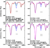 |
Fig. 1 V I lines in stars 2M18200365-3224168 (b26), 2M17532599-2053304 (c5), 2M17224443-2343053 (c10), and 2M17552681-3342729 (c19) computed with [V/Fe]=−0.3 (red), 0.0 (cyan), +0.3 (blue), and final values if different (magenta), compared with the observed spectrum (black). |
4 Iron-peak elements: V, Cr, Mn, Co, Ni, and Cu
We analysed lines of V, Cr, Mn, Co, Ni, and Cu as detailed below. The fits were all carried out visually, adopting convolutions with FWHM from 0.65 to 0.75 Å in the range 15 000–17 000 Å. These full width at half maximum (FWHM) values are compatible with those based on a directly measured FWHM of ~0.7 Å, with 10–20 per cent variations seen across the wavelength range by Ashok et al. (2021) and Nidever et al. (2015). Although for most of the lines the resulting abundance is similar to that reported in DR17, there are cases where the visual inspection is needed because of noise or defects. The results are given in Table A.1.
Vanadium: the V I 15924.791 Å line, together with the weaker line at 15 925.595 Å is measurable; all other lines are too shallow in these metal-poor stars. Hayes et al. (2022) indicate a further two lines, which only appear in stars more metal-rich than those analysed here. Figure 7 of this latter paper shows results for stars with metallicities [Fe/H] > −1.0. In Table A.2, we replace the values of [V/Fe] from the DR 17 results with more reliable measurements from the BACCHUS Analysis of Weak Lines in APOGEE Spectra (BAWLAS). BAWLAS is part of the DR17 release as a Value Added Catalog (VAC Hayes et al. 2022), and presents abundances for some of the elements represented by only weak lines, namely Na, P, S, V, Cu, Ce, and Nd, as well as 12C/13C ratios. The VAC used only spectra with higher signal-to-noise ratios (S/N~120). Figure 1 shows the fit to the V I 15924.791 Å line in four stars: 2M18200365-3224168 (b26), 2M17532599-2053304 (c5), 2M17224443-2343053 (c10), and 2M17552681-3342729 (c19). However, even considering that some of the fits are credible, some noise is present in the region and the plot of [V/Fe] versus [Fe/H] shows a large spread (see Sect. 5).
Chromium: there are four measurable lines, but only two are useful for all stars. This is because, for one-third of the stars, the line at Cr I 15 860.214 Å falls in the instrument gap and the line Cr I 16 015.327 Å is blended with a strong unidentified feature. The latter line is measurable for only a few stars; in the others, it results in a spurious, much higher Cr abundance. Regarding the blends disturbing the 16 015.327 Å line listed in Table 1, Smith et al. (2021) points out possible identifications of a feature at 16 016.75 Å, which could be Ni I, Zr I, or Ni I; it is also blended with a 12C16O line, but the CO lines are taken into account using the proper abundances of C and O from Razera et al. (2022).
We adopted a mean of the Cr abundance from the two measurable lines. With most cases, measured from the Cr I 15 178.593 Å and 15 680.063 Å lines, we adopted the mean obtained from the fits to these lines, or only the fit for the best line, which is Cr I 15 680.063 Å. In some cases, the result is the mean of the three lines (always discarding Cr I 16 015.327 Å, except in one unique star). Figure 2 provides an example of the fits to the Cr lines for the star 2M17382504-2424163 (c17).
Manganese: the three lines listed in the APOGEE reference papers cited above are suitable. Two other lines that we detected are too faint in these metal-poor stars. In general, we find very good agreement with the ASPCAP results (see Table A.2). Figure 3 shows a fit for the 3 Mn I lines in star 2M18200365-3224168 (b26). In cases where the Mn abundance varies among the lines, a mean value was adopted.
Cobalt: Co I 16757.7 Å is the unique suitable line, as listed in Smith et al. (2013), but is a very strong and clean line. We also inspected two other lines, CoI 15 906.075 and 16 568.649 Å, but these were not useful. Figure 4 shows the fit to the Co line in four stars, namely 2M17392719-2310311 (b14), 2M17552744-3228019 (b19), 2M17532599-2053304 (c5), and 2M17503065-2313234 (c28).
Nickel: we analysed nine lines, identified with an asterisk in Table 1, and in general they give the same resulting abundance. For the cases where the result differs from line to line, we adopted a mean Ni abundance. The line Ni I 16 589.440 Å tends to give higher abundances in most stars. Figure 5 shows the fit to the nine lines for star 2M18010424-3126158 (c21).
Copper: the CuI 16 005.735 Å line identified by Smith et al. (2013) is the single useful line. We also identified the CuI 16 650.0 Å line, but the latter is immersed in a strong feature composed of other blending lines; this feature is insensitive to the Cu abundance. The Cu I 16 005.735 Å line is located between a line consisting mainly of Fe I, and a small contribution of Ti I, Ti II, and Ca I lines, and on the red side a strong Fe I line. The Cu I line is on the wing of the bluer feature, and can be checked. The main uncertainty in the Cu abundance is due to the adopted continuum level. Regarding the continuum, we verified the overall fit to the continuum in the region 16 002–16 011 Å and for most stars we used the local continuum at around 16 009 Å situated after the blend dominated by the Fe I 16 006.758 Å line. It is also difficult to measure the extent of the Cu deficiency in the severely Cu-deficient cases. Figure 6 shows the fit to the Cu I 16 005.735 Å line for six stars: 2M17153858-2759467 (b1), 2M17173693-2806495 (b2), 2M17250290-2800385 (b3), 2M17265563-2813558 (b4), 2M17295481-2051262 (b6), and 2M17324257-2301417 (b8).
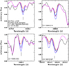 |
Fig. 2 Cr I lines in star 2M17382504-2424163 (c17) computed with [Cr/Fe]=−0.3 (red), 0.0 (cyan), +0.3 (blue), and +0.08 (magenta) compared with the observed spectrum (black). The final result of [Cr/Fe]=+0.08 is shown in magenta. |
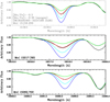 |
Fig. 3 Manganese lines in star 2M18200365-3224168 (b26). The synthetic spectra were computed with [MnFe]=−0.6 (green), −0.3 (red), 0.0 (cyan), and +0.3 (blue), and are compared with the observed spectrum (black). A final value of [MnFe]=−0.3 fits the three lines well. |
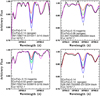 |
Fig. 4 Cobalt line in four stars: 2M17392719-2310311 (b14), 2M17552744-3228019 (b19), 2M17532599-2053304 (c5), and 2M17503065-2313234 (c28). The synthetic spectra were computed with [Co/Fe]=−0.3 (red), 0.0 (cyan), +0.3 (blue), the APOGEE value indicated in the panels (green), and the final value (magenta), and are compared with the observed spectrum (black). |
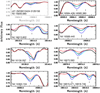 |
Fig. 5 Nickel lines in star 2M18010424-3126158 (c21). The synthetic spectra were computed with [Ni/Fe]=−0.3 (red), 0.0 (cyan), and +0.3 (blue), and are compared with the observed spectrum (black). |
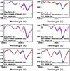 |
Fig. 6 Copper line in six stars illustrating the difficulty in deriving Cu abundances. The synthetic spectra were computed with [Cu/Fe]=−0.3 (red), 0.0 (cyan), +0.3 (blue), and +0.08 (magenta), an are compared with the observed spectrum (black). |
4.1 Non-LTE corrections
Non-local thermodynamic equilibrium (NLTE) corrections are available for some of the lines of Cr, Mn, and Co by Bergemann & Cescutti (2010), Bergemann & Gehren (2008), and Bergemann et al. (2010), provided on their website1. These corrections are reported in Table B.1.
We conducted a detailed examination of the NLTE corrections provided on the MPIA website for the available spectral lines. For Cr I, corrections are available for the lines at 15 680.063, 15 860.214, and 16 015.327 A, with an average correction of ~0.15 dex. An inspection of the curve of growth and the line profiles did not reveal any significant discrepancies. However, there are no corrections for the line 15 178.593 Å, which is one of the only two adopted; in addition, the corrections appear too high, and so we did not apply these NLTE corrections to Cr.
For Mn I, corrections are provided for the lines at 15 217.793 and 15 262.702 Å. The line at 15 217.793 Å exhibits an average correction of ~0.10 dex, whereas the 15 252.702 Å line would have a larger NLTE correction of ~0.5 dex. Therefore, as not all three lines have corrections available, and because the corrections appear reasonable for only one line and high for the rest, we also did not apply NLTE corrections for Mn. The corrections on Co I 16757.711 Å abundances appear suitable, and lead to the finding that Co appears under-abundant at the lower metallicities.
Finally, the papers cited above as used for the NLTE corrections adopt the classical inelastic collisions with the hydrogen atoms by Drawin (1968) in their calculations. The approximation is scaled by a factor SH, which in the Bergemann et al. papers is assumed to have a very low value (SH = 0 for Cr and Mn and SH = 0.05 for Co), thereby maximising the size of the NLTE corrections. For this reason, we finally did not apply the NLTE corrections to the resulting spectroscopic abundances to any of the analysed elements.
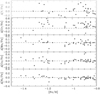 |
Fig. 7 [V, Cr, Mn, Co, Ni/Fe] vs. [Fe/H], plotting the differences between the present results and the APOGEE DR17 values. |
4.2 Uncertainties
The uncertainties in the derived abundances can be seen in Figure 7, where we plot the difference in abundances, that is, the abundances derived in this work minus the ones derived with the APOGEE-ASPCAP DR17 software. The differences between the two measurements can be considered as the uncertainty, which are mainly due to continuum placement.
There is good agreement between the two values for V, Mn, and Co, with V tending to be higher in the present work, and very good agreement regarding the Ni abundances. Finally, the present Cr abundances are systematically higher than the ASPCAP ones.
The mean difference between our results and ASPCAP are found to be:
![Mathematical equation: $\[\begin{align*} {[\mathrm{V} / \mathrm{Fe}]_{\text {present }}-[\mathrm{V} / \mathrm{Fe}]_{\mathrm{ASPCAP}} }=+0.11 \pm 0.005,\\{[\mathrm{Cr} / \mathrm{Fe}]_{\text {present }}-[\mathrm{Cr} / \mathrm{Fe}]_{\mathrm{ASPCAP}} }=+0.17 \pm 0.003,\\{[\mathrm{Mn} / \mathrm{Fe}]_{\text {present }}-[\mathrm{Mn} / \mathrm{Fe}]_{\mathrm{ASPCAP}}=-0.04 \pm 0.001},\\{[\mathrm{Co} / \mathrm{Fe}]_{\text {present }}-[\mathrm{Co} / \mathrm{Fe}]_{\mathrm{ASPCAP}}=+0.03 \pm 0.001},\\{[\mathrm{Ni} / \mathrm{Fe}]_{\text {present }}-[\mathrm{Ni} / \mathrm{Fe}]_{\mathrm{ASPCAP}}=+0.00 \pm 0.0002}.\end{align*} \]$](/articles/aa/full_html/2024/11/aa52235-24/aa52235-24-eq1.png) (1)
(1)
The visual fits are more reliable than ASPCAP for lines in noisy spectra or where lines are too faint, in which case ASPCAP tends to assign very low abundances, and this is the reason for our abundances being higher by +0.11 and +0.17 dex for V and Cr. The VAC-BAWLAS results for vanadium partly mitigate this issue. For Mn, Co, and Ni, the mean difference is low, but the present results appear more homogeneous. The fits are available upon request.
5 Chemical-evolution models
The chemical-evolution model for the Galactic bulge computed here assumes a classical bulge. It is derived from the chemical-evolution models of Friaça & Terlevich (1998), which adopted a multi-zone chemical evolution coupled with a hydrodynamical code. For the Galactic bulge, a classical spheroid with a baryonic mass of 2×10⁹ M⊙ and a dark halo mass of 1.3×10¹⁰ M⊙ are assumed (e.g. Barbuy et al. 2018a).
Cosmological parameters from the Planck Collaboration VI (2020) are adopted, namely Ωm = 0.31, ΩΛ = 0.69, Hubble constant H0= 68 km s−1Mpc−1, and an age of the Universe of 13.801±0.024 Gyr.
For the nucleosynthesis yields, we adopt: (i) for massive stars, the metallicity-dependent yields from core-collapse supernovae (CCSNae)/Supernovae Type II (SNe II) from Woosley & Weaver (1995), with some alterations of the yields following the suggestions of Timmes et al. (1995), and for low metallicities (Z < 0.01 Z⊙, or [Fe/H] < −2.5), the yields are from high-explosion-energy hypernovae (HNe) from Nomoto et al. (2013); (ii) Type Ia Supernovae (SNIa) yields are from Iwamoto et al. (1999) – their models W7 (progenitor star of initial metallicity Z = Z⊙) and W 70 (zero initial metallicity); and (iii) for intermediate-mass stars (0.8–8 M⊙) with initial Z = 0.001, 0.004, 0.008, 0.02, and 0.4, we adopt yields from van den Hoek & Groenewegen (1997) with variable η asymptotic giant branch (AGB case). Models are computed for radii of r < 0.5, 0.5 < r < 1, 1 < r < 2, and 2 < r < 3 kpc from the Galactic centre, and for specific star-formation rate values of ν = 1 and 3 Gyr−1. We note that for Co, the SNe II yields from Woosley & Weaver (1995) were computed both with original values and also multiplied by two, following the recommendations of Timmes et al. (1995), see further discussion below. The yields of SNe Ia for Ni from Iwamoto et al. (1999) were divided by two, because, as the authors pointed out, the W7 model overproduces 58Ni, the main Ni isotope. More over, from Table 3 of Iwamoto et al. (1999), the W7 model has [58Ni/56Fe]=+0.62, and the W70 model, [58Ni/56Fe]=+0.47, whereas the five remaining models have an average [58Ni/56Fe]=+0.14, implying 58Ni overabundances by factors of ~ 3 and ~ 2, for models W7 and W70, respectively.
Below we describe the available literature data for the studied elements, which are taken into account in the [X/Fe] versus [Fe/H] plots, and the chemical-evolution models. Figures 8, 9, and 10 show [V/Fe] versus [Fe/H] (upper panel) and [Mn/Fe] versus [Fe/H] (lower panel), [Cr/Fe] versus [Fe/H] (upper panel) and [Ni/Fe] versus [Fe/H] (lower panel), and [Co/Fe] versus [Fe/H] (upper panel) and [Cu/Fe] versus [Fe/H] (lower panel), respectively. The present data are compared with literature data and the chemical-evolution models described above, that is, for specific star formation rates of νSF = 1 and 3 Gyr−1. The literature data included in these plots are described below.
Vanadium: In Figure 8 (upper panel) the present data are compared with the following literature data: bulge GCs from Ernandes et al. (2018), thick-disc and halo stars from Ishigaki et al. (2013), halo stars from Hawkins et al. (2016a), disc stars from Kepler+APOGEE given in Hawkins et al. (2016b), and bulge field stars by Nandakumar et al. (2024). As most of the available data on V do not correspond to bulge stars, the origin of the different samples is indicated in the figure panel. The data show a large spread.
Manganese: in Figure 8 (lower panel) the present data are compared with literature data, including the GCs from Ernandes et al. 2018, namely the metal-rich bulge clusters NGC 6528 and NGC 6553, the moderately metal-poor clusters HP 1, NGC 6522, and NGC 6558, and additionally the disc cluster 47 Tucanae; again results for the metal-rich cluster NGC 6528 from Sobeck et al. (2006), and the relatively metal-poor cluster NGC 6355 from Souza et al. (2023), and bulge field stars (Nandakumar et al. 2024; Lomaeva et al. 2019; Schultheis et al. 2017; Barbuy et al. 2013; McWilliam et al. 2003). We note that Schultheis et al. (2017) are early results from APOGEE Data Release 13 (DR13). Mn abundances from Lucey et al. (2022) are not plotted because of the large scatter for this element. The models appear to fit the data very well, however we note that the NLTE corrections were not taken into account.
Manganese behaves as a metallicity-dependent element. [Mn/Fe] decreases with decreasing metallicity due to the decreasing trend in the yields from SNe II ejecta at metallicities of lower than [Fe/H] ~ −1. In addition, for solar metallicities, the SNe II Mn yields have almost solar abundances and the SNIa contribution becomes noticeable for [Fe/H]> −0.8. For the W70 model of Iwamoto et al. (1999), [Mn/Fe]= −007, and [Mn/Fe] = +0.10 for the W7 model. The impact of the SNe Ia is clearly seen in Figure 8, in the small jump of [Mn/Fe] at [Fe/H] ~ −0.8, as shown by the chemodynamical model with νSF = 3 Gyr−1.
Chromium: literature data include bulge field stellar abundances (Nandakumar et al. 2024; Lucey et al. 2022; Lomaeva et al. 2019; Bensby et al. 2017; Schultheis et al. 2017; Johnson et al. 2014). Cr tends to vary in lockstep with Fe. The models for Cr show a suprasolar bump at [Fe/H]~−1.1 and a subsolar bow at [Fe/H]~−2.0 as a direct consequence of the yields from Woosley & Weaver (1995). Again, the data presented by Schultheis et al. (2017) are early results from APOGEE DR13.
Cobalt: literature data include bulge field-stars (Nandakumar et al. 2024; Ernandes et al. 2020; Lomaeva et al. 2019; Schultheis et al. 2017; Johnson et al. 2014). Co tends to vary in lockstep with Fe, but could be somewhat under-abundant in the more metalpoor stars, which is not reproduced by the models. In Figure 10, the NLTE Co abundances are taken into account in results from Ernandes et al. (2020), but this is not the case for the present data due to the reasons explained in subsection 4.1. For Co, the data from Schultheis et al. (2017) are early results from APOGEE DR13. The adopted yields from Woosley & Weaver (1995) are shown with original values, but also with Co yields multiplied by two, as recommended by Timmes et al. (1995). It appears that with the new data for the more metal-poor stars, the original yields are more suitable.
Nickel: literature data include bulge field-stars (Nandakumar et al. 2024; Lomaeva et al. 2019; Bensby et al. 2017; Schultheis et al. 2017; Johnson et al. 2014). Regarding the data from Bensby et al. (2017), we adopt only the stars older than 11 Gyr. Schultheis et al. (2017) are early results from APOGEE DR13. Ni clearly varies in lockstep with Fe. Relative to the other elements studied here, the models for Ni follow the Fe more closely, with a deviation from solar ratios at around [Ni/Fe]< ± 0.1. This applies to the models and also to the data.
Copper: literature data include bulge field-stars abundances (Nandakumar et al. 2024; Ernandes et al. 2020; Lomaeva et al. 2019; Xu et al. 2019; Johnson et al. 2014), and GC data are from Ernandes et al. (2018).
In conclusion, Cr and Ni vary in lockstep with Fe, that is, [Cr/Fe] ~ [Ni/Fe] ~ 0.0 for all metallicities. Mn is deficient for metal-poor stars and shows a clear secondary behaviour. Regarding Co and Cu, in Barbuy et al. (2018a) and Ernandes et al. (2020), we suggested that abundances of Co and Cu could be used to discriminate between their origin as neutron capture elements on iron-group nuclei during He burning and later burning stages, also called the weak-s component (Limongi & Chieffi 2003), and the α-rich freeze-out in the deepest layers (Woosley et al. 1973; Woosley & Weaver 1995; Woosley et al. 2002; Sukhbold et al. 2016). The results of Ernandes et al. (2020) seemed to clearly show that Co follows Fe, but only a few points at [Fe/H] ≤ −1 were available to these authors. With the present data, we see that for some stars, Co tends to vary in lockstep with Fe, showing [Co/Fe] ~ 0.0, but there are also several stars with a lower [Co/Fe] for [Fe/H] < −1. As mentioned above, following a suggestion by Timmes et al. (1995), the yields of Co from Woosley & Weaver (1995) multiplied by two satisfy the higher Co values, but for the Co-low more metal-poor stars, the original lower Co yields provide a better fit to the data. This is now evidence that Co, and likewise Cu, might have a secondary behaviour, not being dominantly produced by alpha-rich freezeout as we suggested in Ernandes et al. (2020) but by a weak-s process. Cu shows a clear secondary behaviour, but another issue is that Cu appears to be even more deficient than predicted by the models for [Fe/H]<−0.8.
Finally, Zasowski et al. (2019) studied the APOGEE DR14 and DR15 abundances of 4000 stars located at distances of <4 kpc from the Galactic centre, including Cr, Mn, Co, and Ni. The data naturally show a large spread, but the general trend of Cr, Mn, and Ni is compatible with the present results, whereas their Co abundances show too large a spread to be compared with the present results.
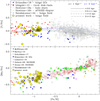 |
Fig. 8 [V/Fe] vs. [Fe/H] (upper panel) and [Mn/Fe] vs. [Fe/H] (lower panel): Chemical-evolution models with SFR of ν = 1 and 3 Gyr−1 (black and blue lines respectively) overplotted on the results of the present study (yellow pentagons) and literature data. Bulge GCs are from Ernandes et al. (2018) (blue squares), bulge field stars are from Nandakumar et al. (2024) (sea green open stars). For V: thick disc and halo stars from Ishigaki et al. (2013) (red filled circles), halo stars from Hawkins et al. (2016a), and disc stars from Kepler+APOGEE given in Hawkins et al. (2016b) (bold grey open stars). For Mn: bulge field data from Lomaeva et al. (2019) (filled orange triangles), Schultheis et al. (2017) (open red circles), Barbuy et al. (2013) (filled green circles), McWilliam et al. (2003) (filled blue triangles), and GCs NGC 6528 by Sobeck et al. (2006) (filled magenta triangles), NGC 6355 by Souza et al. (2023) (filled red triangles). Different model lines correspond to the outputs of models computed for radii r < 0.5, 0.5 < r < 1, 1 < r < 2, and 2 < r < 3 kpc from the Galactic centre. |
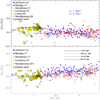 |
Fig. 9 [Cr/Fe] vs. [Fe/H] (upper panel) and [Ni/Fe] vs. [Fe/H] (lower panel). Chemical-evolution models with SFR of ν = 1 and 3 Gyr−1 (black and blue lines respectively) overplotted on the results of the present study (yellow pentagons) and literature data: Johnson et al. (2014) (blue filled circles), Bensby et al. (2017) (red filled circles), Schultheis et al. (2017) (open red circles), Lomaeva et al. (2019) (filled orange triangles), and Lucey et al. (2022) (grey filled circles, only for Ni). Different model lines are for the same radii from the Galactic centre as in Fig. 8. |
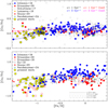 |
Fig. 10 [Co/Fe] vs. [Fe/H] (upper panel) and [Cu/Fe] vs. [Fe/H] (lower panel): Chemical-evolution models with specific star formation of ν = 1 and 3 Gyr−1 for original yields from Woosley & Weaver (1995) (black and blue respectively), and for Co yields multiplied by two (red and magenta lines). Data consist of the present results (yellow pentagons) and literature data, including field data from Johnson et al. (2014) (blue filled circles), Ernandes et al. (2020) (red filled circles), and Schultheis et al. (2017) (open grey circles), and Xu et al. (2019) (filled grey triangles), plus GC data from Ernandes et al. (2018) (red open circles) in the lower panel. Different model lines are for the same radii from the Galactic centre, as in Fig. 8. |
6 Inspecting abundance indicators
Table 2 lists the abundances of elements studied in Razera et al. (2022) and Barbuy et al. (2023). Together with Table A.1, these data gather all abundances verified by our calculations, in addition to that of cerium, which was also analysed in Razera et al. (2022).
We have analysed some of these abundances as indicators of origin as second generation from GCs, and abundance indicators of in situ or ex situ origin.
Nitrogen-rich stars in the bulge field were identified as second-generation stars evaporated from GCs by Schiavon et al. (2017) and Fernández-Trincado et al. (2017). In our sample stars, b15, c11, and C13 are N-rich with [N/Fe]>+0.5, and could be considered as second-generation stars evaporated from GCs. The star c13 also has a rather high Na abundance of [Na/Fe]=+0.35; see Table 2.
We apply the correlations discussed in Montalbán et al. (2021), and Ortigoza-Urdaneta et al. (2023), who proposed that [Ni/Fe] versus [(C+N)/O] is an indicator that can be used to discriminate between an in situ and an ex situ stellar origin, similar to the more popular representation in the [Mg/Mn] versus [Al/Fe] plane. We show both the present abundances and the APOGEE-ASPCAP abundances for the same 58 stars. Figure 11 shows these plots, where we can see that in the [Mg/Mn] versus [Al/Fe] plane there are stars spread between the in situ and the ex situ region. The difference with the Queiroz et al. (2021) population is larger for the results in this study when compared with the DR 17 results that looked more spread between the two regions. In the [Ni/Fe] versus [(C+N)/O] plot, more stars fall in the Heracles locus. For [Mg/Mn] versus [Al/Fe], Queiroz et al. (2021) demonstrated that counter-rotating stars populate both the in situ and ex situ regions. Vasini et al. (2024) demonstrate that the uncertainties on the chemical yields can reproduce totally different star formation histories (SFHs) in the [Mg/Mn] versus [Al/Fe] plane, which means that they may reproduce an ex situ SFH using in situ yields. On the other hand, Feltzing & Feuillet (2023) argue that this kind of plot can lead to a clear separation between in situ metalweak disc and halo ex situ stars, which otherwise also show a high and moderate [Mg/Fe], respectively. As for Ni, subsolar Ni is expected for ex situ stars, whereas [Ni/Fe] = 0.00 ± 0.05 for our sample, which is characteristic of an in situ origin. Second-generation stars can also mimic an in situ origin on the [Mg/Mn] versus [Al/Fe] plane, as observed by Fernández-Trincado et al. (2022) and Souza et al. (2023), who analysed individual stars of in situ GCs. For instance, the GC NGC 6558, classified as in situ based on different methods (Barbuy et al. 2018b; Pérez-Villegas et al. 2020; Souza et al. 2024), has stars with low [Al/Fe], which could lead to a misinterpretation that NGC 6558 is an ex situ cluster, if only this criterion were taken into account.
Nissen et al. (2024) point out a parallel between the abundances of alpha elements and iron-peak elements. For their alpha-low stars, V, Sc, and Co are also low. Our stars are all alpha-enhanced, as can be seen from their O and Mg abundances, and somewhat lower values of Ca and Si – this is expected given that O and Mg are produced in hydrostatic phases of massive stars, whereas Ca and Si are produced in explosive phases (McWilliam 2016). For Nissen’s stars, the alpha-enhanced stars show [Co/Fe]~+0.1, like most of our stars, and the alpha-low ones show [Co/Fe] ~ −0.1. Also, Nissen & Schuster (2010) found that nearly all accreted stars in the solar neighbourhood have −0.2 < [Ni/Fe] < −0.05. Our sample stars are all alpha-enhanced and most of them also show [Co/Fe]~+0.0 to 0.1, and [Ni/Fe] ~ 0.0, therefore indicating an in situ origin.
In conclusion, we believe that [(C+N)/O] does not seem to offer a robust way of discriminating between an ex situ and an in situ origin, as it contradicts the other more reliable indicators such as alpha-enhancement, but also [Al/Fe], which is low in Heracles stars (−0.25 ≲ [Al/Fe] ≲ 0.0). CNO also depends critically on stellar evolution processes of mixing and extra-mixing (e.g. Smiljanic et al. 2009; Shetrone et al. 2019), whereas the other abundance indicators depend on the nucleosynthesis that took place in the environment where the stars were born.
As Heracles selection criteria include high eccentricities and lower energies, some overlap with our selection criteria for selecting our RPM sample (see Queiroz et al. 2020, 2021) is expected.
There are coincidences with Heracles, with however one discriminator being the low [Al/Fe] in Heracles stars. This structure might well be an early progenitor of the early bulge of the Milky Way, and not an accreted object. A similar case is Aurora, which shows a wide range in [Al/Fe], and was considered by Myeong et al. (2022) to contain early stars formed in the young Milky Way.
Abundances of C, N, and O (Razera et al. 2022), Na and Al (Barbuy et al. 2023), and Mg, Si, and Ca from DR17.
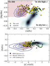 |
Fig. 11 [Mg/Mn] vs. [Al/Fe] (upper panel) and [Ni/Fe] vs. [C+N/O] (lower panel). Contours correspond to Heracles Horta et al. (2021) and Gaia-Sausage-Enceladus Limberg et al. (2022), and the black points to the RPM sample from Queiroz et al. (2021). Yellow pentagons show abundances derived from the results presented here, while blue stars show APOGEE-ASPCAP abundances for the same 58 stars. |
6 Conclusions
This is the third paper of a series dealing with the chemical abundance analysis of 58 stars selected to have [Fe/H]<−0.8 and orbits compatible with being members of a spheroidal component of the Galactic bulge. In the present work, we have recomputed the abundances of the iron-peak elements V, Cr, Mn, Co, Ni, and Cu in spectra observed by the APOGEE collaboration. We confirm which lines are suitable for the determination of these abundances in the range of metallicities of −2.0 < [Fe/H] < −0.8.
The abundances were compared with chemical-evolution models, which appear to reproduce the [X/Fe] versus [Fe/H] behaviour well in most cases. In summary, V, Cr, and Ni tend to vary in lockstep with iron, as does Co, although the present data on Co show a trend towards under-abundance for [Fe/H] <−1, and might be showing a secondary behaviour similar to that of Cu. Mn and Cu decrease with decreasing metallicity, and Cu appears to drop faster than the models predict for [Fe/H]<−0.8. Finally, using abundance discriminators, together with kinematical and dynamical criteria, our sample of 58 stars has the characteristics of an in situ sample.
Acknowledgements
B.B. and A.C.S.F. acknowledge grants from FAPESP, Conselho Nacional de Desenvolvimento Científico e Tecnológico (CNPq) and Coordenação de Aperfeiçoamento de Pessoal de Nível Superior (CAPES) - Financial code 001. P.S. acknowledges Fundação de Amparo à Pesquisa do Estado de São Paulo (FAPESP) post-doctoral fellowships 2020/13239-5 and 2022/14382-1. S.O.S. acknowledges a FAPESP PhD fellowship no. 2018/220443. A.P.-V., B.B., and S.O.S. acknowledge the DGAPA-PAPIIT grant IA103224. P.S., B.B., H.E., and S.O.S. are part of the Brazilian Participation Group (BPG) in the Sloan Digital Sky Survey (SDSS), from the Laboratório Interinstitucional de e-Astronomia – LIneA, Brazil. J.G.F-.T. gratefully acknowledges the grant support provided by Proyecto Fondecyt Iniciación No. 11220340, Proyecto Fondecyt Postdoc No. 3230001 (Sponsored by J.G.F-.T.) and from the Joint Committee ESO-Government of Chile 2021 (ORP 023/2021), and 2023 (ORP 062/2023). F.A. acknowledges partial supported by the Spanish MICIN/AEI/10.13039/501100011033 and by “ERDF A way of making Europe” by the “European Union” through grant PID2021-122842OB-C21, and the Institute of Cosmos Sciences University of Barcelona (ICCUB, Unidad de Excelencia ‘María de Maeztu’) through grant CEX2019-000918-M. FA acknowledges the grant RYC2021-031683-I funded by MCIN/AEI/10.13039/501100011033 and by the European Union NextGenerationEU/PRTR. D.M. gratefully acknowledges support from the Center for Astrophysics and Associated Technologies (CATA) by ANID BASAL projects ACE210002 and FB210003, and Fondecyt Project No. 1220724. D.G. gratefully acknowledges the support provided by Fondecyt regular n. 1220264. D.G. also acknowledges financial support from the Dirección de Investigación y Desarrollo de la Universidad de La Serena through the Programa de Incentivo a la Investigación de Académicos (PIA-DIDULS). The work of V.V.S. and V.M.P. is supported by NOIRLab, which is managed by the Association of Universities for Research in Astronomy (AURA) under a cooperative agreement with the U.S. National Science Foundation. T.C.B. acknowledges support from grant PHY 14-30152; Physics Frontier Center/JINA Center for the Evolution of the Elements (JINA-CEE), and from OISE-1927130: The International Research Network for Nuclear Astrophysics (IReNA), awarded by the US National Science Foundation. Apogee project: funding for the Sloan Digital Sky Survey IV has been provided by the Alfred P. Sloan Foundation, the U.S. Department of Energy Office of Science, and the Participating Institutions. SDSS acknowledges support and resources from the Center for High-Performance Computing at the University of Utah. The SDSS web site is www.sdss.org. SDSS is managed by the Astrophysical Research Consortium for the Participating Institutions of the SDSS Collaboration including the Brazilian Participation Group, the Carnegie Institution for Science, Carnegie Mellon University, Center for Astrophysics I Harvard & Smithsonian (CfA), the Chilean Participation Group, the French Participation Group, Instituto de Astrofísica de Canarias, The Johns Hopkins University, Kavli Institute for the Physics and Mathematics of the Universe (IPMU) / University of Tokyo, the Korean Participation Group, Lawrence Berkeley National Laboratory, Leibniz Institut für Astrophysik Potsdam (AIP), Max-Planck-Institut für Astronomie (MPIA Heidelberg), Max-Planck-Institut für Astrophysik (MPA Garching), Max-Planck-Institut für Extraterrestrische Physik (MPE), National Astronomical Observatories of China, New Mexico State University, New York University, University of Notre Dame, Observatório Nacional / MCTI, The Ohio State University, Pennsylvania State University, Shanghai Astronomical Observatory, United Kingdom Participation Group, Universidad Nacional Autónoma de México, University of Arizona, University of Colorado Boulder, University of Oxford, University of Portsmouth, University of Utah, University of Virginia, University of Washington, University of Wisconsin, Vanderbilt University, and Yale University.
Appendix A Present and APOGEE-ASPCAP abundance results
In Table A.1 are given the APOGEE uncalibrated stellar parameters, and the present resulting abundances for the elements V, Cr, Mn, Co, Ni, and Cu. In Table A.2 we report the abundances of V, Cr, Mn, Co, and Ni from APOGEE DR 17 for the 58 sample stars. Copper was not measured by the APOGEE ASPCAP procedure. The values in bold face correspond to data from the Value Added Catalog (VAC), and analysed in BAWLAS (see text).
Appendix B Non-Local thermodynamic Equilibrium corrections
Table B.1 provides the NLTE corrections for the lines available in Bergemann & Cescutti (2010), for the elements Cr, Mn, and Co. We only adopted the final values for the Co abundances, given that for Cr and Mn there are no corrections for all the lines studied, and for Cr and Mn the corrections appear too high.
Stellar parameters and abundances of V, Cr, Mn, Co, Ni, and Cu derived.
Abundances of V, Cr, Mn, Co, and Ni from APOGEE DR17 for the 58 sample stars.
NLTE corrections (in dex) for the Cr I, Mn I, Co I lines available in nlte.mpia.de website.
References
- Abdurro’uf, Accetta, K., Aerts, C., et al. 2022, ApJS, 259, 35 [NASA ADS] [CrossRef] [Google Scholar]
- Allende Prieto, C., Beers, T. C., Wilhelm, R., et al. 2006, ApJ, 636, 804 [NASA ADS] [CrossRef] [Google Scholar]
- Alvarez, R., & Plez, B. 1998, A&A, 330, 1109 [NASA ADS] [Google Scholar]
- Ashok, A., Zasowski, G., Seth, A., et al. 2021, AJ, 161, 167 [NASA ADS] [CrossRef] [Google Scholar]
- Asplund, M., Amarsi, A. M., & Grevesse, N. 2021, A&A, 653, A141 [NASA ADS] [CrossRef] [EDP Sciences] [Google Scholar]
- Athanassoula, E., Rodionov, S. A., & Prantzos, N. 2017, MNRAS, 467, L46 [Google Scholar]
- Babusiaux, C., Gómez, A., Hill, V., et al. 2010, A&A, 519, A77 [NASA ADS] [CrossRef] [EDP Sciences] [Google Scholar]
- Barbuy, B., Hill, V., Zoccali, M., et al. 2013, A&A, 559, A5 [NASA ADS] [CrossRef] [EDP Sciences] [Google Scholar]
- Barbuy, B., Chiappini, C., & Gerhard, O. 2018a, ARA&A, 56, 223 [Google Scholar]
- Barbuy, B., Muniz, L., Ortolani, S., et al. 2018b, A&A, 619, A178 [NASA ADS] [CrossRef] [EDP Sciences] [Google Scholar]
- Barbuy, B., Friaça, A. C. S., Ernandes, H., et al. 2023, MNRAS, 526, 2365 [NASA ADS] [CrossRef] [Google Scholar]
- Beaton, R. L., Oelkers, R. J., Hayes, C. R., et al. 2021, AJ, 162, 302 [NASA ADS] [CrossRef] [Google Scholar]
- Belokurov, V., Erkal, D., Evans, N. W., Koposov, S. E., & Deason, A. J. 2018, MNRAS, 478, 611 [Google Scholar]
- Belokurov, V., & Kravtsov, A. 2023, MNRAS, 525, 4456 [NASA ADS] [CrossRef] [Google Scholar]
- Bensby, T., Feltzing, S., Gould, A., et al. 2017, A&A, 605, A89 [NASA ADS] [CrossRef] [EDP Sciences] [Google Scholar]
- Bergemann, M., & Cescutti, G. 2010, A&A, 522, A9 [NASA ADS] [CrossRef] [EDP Sciences] [Google Scholar]
- Bergemann, M., & Gehren, T. 2008, A&A, 492, 823 [NASA ADS] [CrossRef] [EDP Sciences] [Google Scholar]
- Bergemann, M., Pickering, J. C., & Gehren, T. 2010, MNRAS, 401, 1334 [CrossRef] [Google Scholar]
- Bica, E., Ortolani, S., & Barbuy, B. 2016, PASA, 33, e028 [Google Scholar]
- Bica, E., Ortolani, S., Barbuy, B., & Oliveira, R. A. P. 2024, A&A, 687, A201 [NASA ADS] [CrossRef] [EDP Sciences] [Google Scholar]
- Blanton, M. R., Bershady, M. A., Abolfathi, B., et al. 2017, AJ, 154, 28 [Google Scholar]
- Bowen, I. S., & Vaughan, A. H. J., 1973, Appl. Opt., 12, 1430 [Google Scholar]
- Chiappini, C., Frischknecht, U., Meynet, G., et al. 2011, Nature, 472, 454 [Google Scholar]
- da Silva, P., Barbuy, B., Ernandes, H., et al. 2024, A&A, 687, A66 [NASA ADS] [CrossRef] [EDP Sciences] [Google Scholar]
- Debattista, V. P., Ness, M., Gonzalez, O. A., et al. 2017, MNRAS, 469, 1587 [Google Scholar]
- Drawin, H.-W. 1968, Zeitschrift für Physik A Hadrons and nuclei, 211, 404 [CrossRef] [Google Scholar]
- Ernandes, H., Barbuy, B., Alves-Brito, A., et al. 2018, A&A, 616, A18 [NASA ADS] [CrossRef] [EDP Sciences] [Google Scholar]
- Ernandes, H., Barbuy, B., Friaça, A. C. S., et al. 2020, A&A, 640, A89 [NASA ADS] [CrossRef] [EDP Sciences] [Google Scholar]
- Feltzing, S., & Feuillet, D. 2023, ApJ, 953, 143 [NASA ADS] [CrossRef] [Google Scholar]
- Fernández-Trincado, J. G., Zamora, O., García-Hernández, D. A., et al. 2017, ApJ, 846, L2 [Google Scholar]
- Fernández-Trincado, J. G., Beers, T. C., Barbuy, B., et al. 2022, A&A, 663, A126 [NASA ADS] [CrossRef] [EDP Sciences] [Google Scholar]
- Forbes, D. A. 2020, MNRAS, 493, 847 [Google Scholar]
- Friaça, A. C. S., & Terlevich, R. J. 1998, MNRAS, 298, 399 [CrossRef] [Google Scholar]
- Gaia Collaboration (Brown, A. G. A., et al.) 2021, A&A, 649, A1 [NASA ADS] [CrossRef] [EDP Sciences] [Google Scholar]
- Gao, L., Theuns, T., Frenk, C. S., et al. 2010, MNRAS, 403, 1283 [CrossRef] [Google Scholar]
- García Pérez, A. E., Allende Prieto, C., Holtzman, J. A., et al. 2016, AJ, 151, 144 [Google Scholar]
- Gunn, J. E., Siegmund, W. A., Mannery, E. J., et al. 2006, AJ, 131, 2332 [NASA ADS] [CrossRef] [Google Scholar]
- Gustafsson, B., Edvardsson, B., Eriksson, K., et al. 2008, A&A, 486, 951 [NASA ADS] [CrossRef] [EDP Sciences] [Google Scholar]
- Hawkins, K., Jofré, P., Heiter, U., et al. 2016a, A&A, 592, A70 [NASA ADS] [CrossRef] [EDP Sciences] [Google Scholar]
- Hawkins, K., Masseron, T., Jofré, P., et al. 2016b, A&A, 594, A43 [NASA ADS] [CrossRef] [EDP Sciences] [Google Scholar]
- Hayes, C. R., Masseron, T., Sobeck, J., et al. 2022, ApJS, 262, 34 [NASA ADS] [CrossRef] [Google Scholar]
- Helmi, A., Babusiaux, C., Koppelman, H. H., et al. 2018, Nature, 563, 85 [Google Scholar]
- Horta, D., Schiavon, R. P., Mackereth, J. T., et al. 2021, MNRAS, 500, 1385 [Google Scholar]
- Hubeny, I., & Lanz, T. 2017, arXiv e-prints [arXiv:1706.01859] [Google Scholar]
- Hubeny, I., Allende Prieto, C., Osorio, Y., & Lanz, T. 2021, arXiv e-prints [arXiv:2104.02829] [Google Scholar]
- Ishigaki, M. N., Aoki, W., & Chiba, M. 2013, ApJ, 771, 67 [NASA ADS] [CrossRef] [Google Scholar]
- Iwamoto, K., Brachwitz, F., Nomoto, K., et al. 1999, ApJS, 125, 439 [NASA ADS] [CrossRef] [Google Scholar]
- Johnson, C. I., Rich, R. M., Kobayashi, C., Kunder, A., & Koch, A. 2014, AJ, 148, 67 [Google Scholar]
- Kruijssen, J. M. D., Pfeffer, J. L., Reina-Campos, M., Crain, R. A., & Bastian, N. 2019, MNRAS, 486, 3180 [Google Scholar]
- Kurucz, R., & Bell, B. 1995, Robert Kurucz CD-ROM (Cambridge, Mass.: Smithsonian Astrophysical Observatory), 23 [Google Scholar]
- Limberg, G., Souza, S. O., Pérez-Villegas, A., et al. 2022, ApJ, 935, 109 [NASA ADS] [CrossRef] [Google Scholar]
- Limongi, M., & Chieffi, A. 2003, ApJ, 592, 404 [CrossRef] [Google Scholar]
- Lomaeva, M., Jönsson, H., Ryde, N., Schultheis, M., & Thorsbro, B. 2019, A&A, 625, A141 [NASA ADS] [CrossRef] [EDP Sciences] [Google Scholar]
- Lucey, M., Hawkins, K., Ness, M., et al. 2021, MNRAS, 501, 5981 [NASA ADS] [CrossRef] [Google Scholar]
- Lucey, M., Hawkins, K., Ness, M., et al. 2022, MNRAS, 509, 122 [Google Scholar]
- Majewski, S. R., Schiavon, R. P., Frinchaboy, P. M., et al. 2017, AJ, 154, 94 [NASA ADS] [CrossRef] [Google Scholar]
- Matteucci, F. 2021, A&A Rev., 29, 5 [NASA ADS] [CrossRef] [Google Scholar]
- McWilliam, A. 2016, PASA, 33, e040 [NASA ADS] [CrossRef] [Google Scholar]
- McWilliam, A., Rich, R. M., & Smecker-Hane, T. A. 2003, ApJ, 592, L21 [NASA ADS] [CrossRef] [Google Scholar]
- Montalbán, J., Mackereth, J. T., Miglio, A., et al. 2021, Nat. Astron., 5, 640 [Google Scholar]
- Myeong, G. C., Belokurov, V., Aguado, D. S., et al. 2022, ApJ, 938, 21 [NASA ADS] [CrossRef] [Google Scholar]
- Nandakumar, G., Ryde, N., Mace, G., et al. 2024, ApJ, 964, 96 [NASA ADS] [CrossRef] [Google Scholar]
- Nelder, J. A., & Mead, H. 1965, Comput. J., 7, 308 [CrossRef] [Google Scholar]
- Nidever, D. L., Holtzman, J. A., Allende Prieto, C., et al. 2015, AJ, 150, 173 [NASA ADS] [CrossRef] [Google Scholar]
- Nissen, P. E., & Schuster, W. J. 2010, A&A, 511, L10 [NASA ADS] [CrossRef] [EDP Sciences] [Google Scholar]
- Nissen, P. E., Amarsi, A. M., Skúladóttir, Á., & Schuster, W. J. 2024, A&A, 682, A116 [NASA ADS] [CrossRef] [EDP Sciences] [Google Scholar]
- Nomoto, K., Kobayashi, C., & Tominaga, N. 2013, ARA&A, 51, 457 [CrossRef] [Google Scholar]
- Ortigoza-Urdaneta, M., Vieira, K., Fernández-Trincado, J. G., et al. 2023, A&A, 676, A140 [NASA ADS] [CrossRef] [EDP Sciences] [Google Scholar]
- Pérez-Villegas, A., Barbuy, B., Kerber, L. O., et al. 2020, MNRAS, 491, 3251 [Google Scholar]
- Planck Collaboration VI. 2020, A&A, 641, A6 [NASA ADS] [CrossRef] [EDP Sciences] [Google Scholar]
- Plez, B. 2012, Astrophysics Source Code Library [record ascl:1205.004] [Google Scholar]
- Queiroz, A. B. A., Anders, F., Santiago, B. X., et al. 2018, MNRAS, 476, 2556 [Google Scholar]
- Queiroz, A. B. A., Anders, F., Chiappini, C., et al. 2020, A&A, 638, A76 [NASA ADS] [CrossRef] [EDP Sciences] [Google Scholar]
- Queiroz, A. B. A., Chiappini, C., Perez-Villegas, A., et al. 2021, A&A, 656, A156 [NASA ADS] [CrossRef] [EDP Sciences] [Google Scholar]
- Razera, R., Barbuy, B., Moura, T. C., et al. 2022, MNRAS, 517, 4590 [CrossRef] [Google Scholar]
- Rojas-Arriagada, A., Zoccali, M., Schultheis, M., et al. 2019, A&A, 626, A16 [NASA ADS] [CrossRef] [EDP Sciences] [Google Scholar]
- Rossi, L. J., Ortolani, S., Barbuy, B., Bica, E., & Bonfanti, A. 2015, MNRAS, 450, 3270 [NASA ADS] [CrossRef] [Google Scholar]
- Ryabchikova, T., & Pakhomov, Y. 2015, Balt. Astron., 24, 453 [Google Scholar]
- Sales-Silva, J. V., Cunha, K., Smith, V. V., et al. 2024, ApJ, 965, 119 [NASA ADS] [CrossRef] [Google Scholar]
- Santana, F. A., Beaton, R. L., Covey, K. R., et al. 2021, AJ, 162, 303 [NASA ADS] [CrossRef] [Google Scholar]
- Santiago, B. X., Brauer, D. E., Anders, F., et al. 2016, A&A, 585, A42 [NASA ADS] [CrossRef] [EDP Sciences] [Google Scholar]
- Schiavon, R. P., Zamora, O., Carrera, R., et al. 2017, MNRAS, 465, 501 [Google Scholar]
- Schultheis, M., Rojas-Arriagada, A., García Pérez, A. E., et al. 2017, A&A, 600, A14 [NASA ADS] [CrossRef] [EDP Sciences] [Google Scholar]
- Shetrone, M., Tayar, J., Johnson, J. A., et al. 2019, ApJ, 872, 137 [NASA ADS] [CrossRef] [Google Scholar]
- Smiljanic, R., Gauderon, R., North, P., et al. 2009, A&A, 502, 267 [NASA ADS] [CrossRef] [EDP Sciences] [Google Scholar]
- Smith, V. V., Cunha, K., Shetrone, M. D., et al. 2013, ApJ, 765, 16 [Google Scholar]
- Smith, V. V., Bizyaev, D., Cunha, K., et al. 2021, AJ, 161, 254 [NASA ADS] [CrossRef] [Google Scholar]
- Sobeck, J. S., Ivans, I. I., Simmerer, J. A., et al. 2006, AJ, 131, 2949 [Google Scholar]
- Souza, S. O., Ernandes, H., Valentini, M., et al. 2023, A&A, 671, A45 [NASA ADS] [CrossRef] [EDP Sciences] [Google Scholar]
- Souza, S. O., Libralato, M., Nardiello, D., et al. 2024, A&A, 690, A37 [NASA ADS] [CrossRef] [EDP Sciences] [Google Scholar]
- Sukhbold, T., Ertl, T., Woosley, S. E., Brown, J. M., & Janka, H. T. 2016, ApJ, 821, 38 [NASA ADS] [CrossRef] [Google Scholar]
- Timmes, F. X., Woosley, S. E., & Weaver, T. A. 1995, ApJS, 98, 617 [NASA ADS] [CrossRef] [Google Scholar]
- van den Hoek, L. B., & Groenewegen, M. A. T. 1997, A&AS, 123, 305 [NASA ADS] [CrossRef] [EDP Sciences] [Google Scholar]
- Vasini, A., Spitoni, E., & Matteucci, F. 2024, A&A, 683, A121 [NASA ADS] [CrossRef] [EDP Sciences] [Google Scholar]
- Wilson, J. C., Hearty, F. R., Skrutskie, M. F., et al. 2019, PASP, 131, 055001 [NASA ADS] [CrossRef] [Google Scholar]
- Wise, J. H., Turk, M. J., Norman, M. L., & Abel, T. 2012, ApJ, 745, 50 [NASA ADS] [CrossRef] [Google Scholar]
- Woosley, S. E., & Weaver, T. A. 1995, AIP Conf. Ser., 327, 365 [NASA ADS] [CrossRef] [Google Scholar]
- Woosley, S. E., Arnett, W. D., & Clayton, D. D. 1973, ApJS, 26, 231 [NASA ADS] [CrossRef] [Google Scholar]
- Woosley, S. E., Heger, A., & Weaver, T. A. 2002, Rev. Mod. Phys., 74, 1015 [NASA ADS] [CrossRef] [Google Scholar]
- Xu, X. D., Shi, J. R., & Yan, H. L. 2019, ApJ, 875, 142 [NASA ADS] [CrossRef] [Google Scholar]
- Zasowski, G., Schultheis, M., Hasselquist, S., et al. 2019, ApJ, 870, 138 [NASA ADS] [CrossRef] [Google Scholar]
- Zoccali, M., Vasquez, S., Gonzalez, O. A., et al. 2017, A&A, 599, A12 [NASA ADS] [CrossRef] [EDP Sciences] [Google Scholar]
All Tables
Abundances of C, N, and O (Razera et al. 2022), Na and Al (Barbuy et al. 2023), and Mg, Si, and Ca from DR17.
NLTE corrections (in dex) for the Cr I, Mn I, Co I lines available in nlte.mpia.de website.
All Figures
|
Fig. 1 V I lines in stars 2M18200365-3224168 (b26), 2M17532599-2053304 (c5), 2M17224443-2343053 (c10), and 2M17552681-3342729 (c19) computed with [V/Fe]=−0.3 (red), 0.0 (cyan), +0.3 (blue), and final values if different (magenta), compared with the observed spectrum (black). |
| In the text | |
|
Fig. 2 Cr I lines in star 2M17382504-2424163 (c17) computed with [Cr/Fe]=−0.3 (red), 0.0 (cyan), +0.3 (blue), and +0.08 (magenta) compared with the observed spectrum (black). The final result of [Cr/Fe]=+0.08 is shown in magenta. |
| In the text | |
|
Fig. 3 Manganese lines in star 2M18200365-3224168 (b26). The synthetic spectra were computed with [MnFe]=−0.6 (green), −0.3 (red), 0.0 (cyan), and +0.3 (blue), and are compared with the observed spectrum (black). A final value of [MnFe]=−0.3 fits the three lines well. |
| In the text | |
|
Fig. 4 Cobalt line in four stars: 2M17392719-2310311 (b14), 2M17552744-3228019 (b19), 2M17532599-2053304 (c5), and 2M17503065-2313234 (c28). The synthetic spectra were computed with [Co/Fe]=−0.3 (red), 0.0 (cyan), +0.3 (blue), the APOGEE value indicated in the panels (green), and the final value (magenta), and are compared with the observed spectrum (black). |
| In the text | |
|
Fig. 5 Nickel lines in star 2M18010424-3126158 (c21). The synthetic spectra were computed with [Ni/Fe]=−0.3 (red), 0.0 (cyan), and +0.3 (blue), and are compared with the observed spectrum (black). |
| In the text | |
|
Fig. 6 Copper line in six stars illustrating the difficulty in deriving Cu abundances. The synthetic spectra were computed with [Cu/Fe]=−0.3 (red), 0.0 (cyan), +0.3 (blue), and +0.08 (magenta), an are compared with the observed spectrum (black). |
| In the text | |
|
Fig. 7 [V, Cr, Mn, Co, Ni/Fe] vs. [Fe/H], plotting the differences between the present results and the APOGEE DR17 values. |
| In the text | |
|
Fig. 8 [V/Fe] vs. [Fe/H] (upper panel) and [Mn/Fe] vs. [Fe/H] (lower panel): Chemical-evolution models with SFR of ν = 1 and 3 Gyr−1 (black and blue lines respectively) overplotted on the results of the present study (yellow pentagons) and literature data. Bulge GCs are from Ernandes et al. (2018) (blue squares), bulge field stars are from Nandakumar et al. (2024) (sea green open stars). For V: thick disc and halo stars from Ishigaki et al. (2013) (red filled circles), halo stars from Hawkins et al. (2016a), and disc stars from Kepler+APOGEE given in Hawkins et al. (2016b) (bold grey open stars). For Mn: bulge field data from Lomaeva et al. (2019) (filled orange triangles), Schultheis et al. (2017) (open red circles), Barbuy et al. (2013) (filled green circles), McWilliam et al. (2003) (filled blue triangles), and GCs NGC 6528 by Sobeck et al. (2006) (filled magenta triangles), NGC 6355 by Souza et al. (2023) (filled red triangles). Different model lines correspond to the outputs of models computed for radii r < 0.5, 0.5 < r < 1, 1 < r < 2, and 2 < r < 3 kpc from the Galactic centre. |
| In the text | |
|
Fig. 9 [Cr/Fe] vs. [Fe/H] (upper panel) and [Ni/Fe] vs. [Fe/H] (lower panel). Chemical-evolution models with SFR of ν = 1 and 3 Gyr−1 (black and blue lines respectively) overplotted on the results of the present study (yellow pentagons) and literature data: Johnson et al. (2014) (blue filled circles), Bensby et al. (2017) (red filled circles), Schultheis et al. (2017) (open red circles), Lomaeva et al. (2019) (filled orange triangles), and Lucey et al. (2022) (grey filled circles, only for Ni). Different model lines are for the same radii from the Galactic centre as in Fig. 8. |
| In the text | |
|
Fig. 10 [Co/Fe] vs. [Fe/H] (upper panel) and [Cu/Fe] vs. [Fe/H] (lower panel): Chemical-evolution models with specific star formation of ν = 1 and 3 Gyr−1 for original yields from Woosley & Weaver (1995) (black and blue respectively), and for Co yields multiplied by two (red and magenta lines). Data consist of the present results (yellow pentagons) and literature data, including field data from Johnson et al. (2014) (blue filled circles), Ernandes et al. (2020) (red filled circles), and Schultheis et al. (2017) (open grey circles), and Xu et al. (2019) (filled grey triangles), plus GC data from Ernandes et al. (2018) (red open circles) in the lower panel. Different model lines are for the same radii from the Galactic centre, as in Fig. 8. |
| In the text | |
|
Fig. 11 [Mg/Mn] vs. [Al/Fe] (upper panel) and [Ni/Fe] vs. [C+N/O] (lower panel). Contours correspond to Heracles Horta et al. (2021) and Gaia-Sausage-Enceladus Limberg et al. (2022), and the black points to the RPM sample from Queiroz et al. (2021). Yellow pentagons show abundances derived from the results presented here, while blue stars show APOGEE-ASPCAP abundances for the same 58 stars. |
| In the text | |
Current usage metrics show cumulative count of Article Views (full-text article views including HTML views, PDF and ePub downloads, according to the available data) and Abstracts Views on Vision4Press platform.
Data correspond to usage on the plateform after 2015. The current usage metrics is available 48-96 hours after online publication and is updated daily on week days.
Initial download of the metrics may take a while.