| Issue |
A&A
Volume 696, April 2025
|
|
|---|---|---|
| Article Number | A154 | |
| Number of page(s) | 10 | |
| Section | Galactic structure, stellar clusters and populations | |
| DOI | https://doi.org/10.1051/0004-6361/202451793 | |
| Published online | 16 April 2025 | |
CAPOS: The bulge Cluster APOgee Survey
V. Elemental abundances of the bulge globular cluster HP 1
1
Departamento de Astronomía, Universidad de Concepción,
Casilla 160-C,
Concepcion,
Chile
2
Universidad Sergio Arboleda, Departamento de Matemáticas, Escuela de Ciencias Exactas e Ingenierías,
calle 74 # 14-14,
Bogotá,
Colombia
3
Observatorio Astronómico Nacional, Universidad Nacional de Colombia,
Bogotá,
Colombia
4
Departamento de Física, Facultad de Ciencias, Pontificia Universidad Javeriana,
Cr. 7 No 40–62,
Bogotá
D.C.
110231,
Colombia
5
Universidad Andres Bello, Facultad de Ciencias Exactas, Departamento de Física y Astronomía – Instituto de Astrofísica, Autopista Concepción-Talcahuano
7100,
Talcahuano,
Chile
6
Department of Astronomy, Facultad de Ciencias, Universidad de La Serena,
Av. Juan Cisternas 1200,
La Serena,
Chile
7
Instituto de Astronomía, Universidad Católica del Norte,
Av. Angamos 0610,
Antofagasta,
Chile
★ Corresponding authors; This email address is being protected from spambots. You need JavaScript enabled to view it.
; This email address is being protected from spambots. You need JavaScript enabled to view it.
Received:
5
August
2024
Accepted:
2
March
2025
Abstract
We performed a detailed abundance analysis of ten red giant members of the heavily obscured bulge globular cluster HP 1 using high-resolution, high S/N, near-infrared spectra collected with the Apache Point Observatory Galactic Evolution Experiment II survey (APOGEE-2), obtained as part of the bulge Cluster APOgee Survey (CAPOS). We investigated the chemical abundances for a variety of species, including the light (C, N), odd-Z (Al), α (O, Mg, Si, S, Ca, and Ti), Fe-peak (Ni, Fe), and neutron-capture (Ce) elements. The derived mean cluster metallicity is [Fe/H] = −1.15 ± 0.03, with no evidence of an intrinsic metallicity spread. HP 1 exhibits a typical α enrichment that follows the trend for similar metallicity Galactic globular clusters (GCs), such as NGC 288 and NGC 5904, although our [Si/Fe] abundances are relatively high. We find a significant nitrogen spread (~1 dex) and a large fraction of nitrogen-enhanced ([N/Fe] > +0.7) stars that populate the cluster. We also detect intrinsic star-to-star spreads in [C/Fe], [O/Fe], [Al/Fe], and [Ca/Fe], which are (anti)correlated with several chemical species, indicating the prevalence of the multiple-population phenomenon in HP 1. We uncover for the first time a possible correlation between Ca and Al, although the sample is small. The mean ⟨[Mg/Fe]⟩ = +0.29 and ⟨[Al/Fe]⟩ = +0.46 place HP 1 in the region dominated by in situ GCs, supporting the in situ nature of this cluster.
Key words: techniques: spectroscopic / surveys / stars: abundances / Galaxy: bulge / globular clusters: individual: HP 1
© The Authors 2025
 Open Access article, published by EDP Sciences, under the terms of the Creative Commons Attribution License (https://creativecommons.org/licenses/by/4.0), which permits unrestricted use, distribution, and reproduction in any medium, provided the original work is properly cited.
This article is published in open access under the Subscribe to Open model. This email address is being protected from spambots. You need JavaScript enabled to view it. to support open access publication.
1 Introduction
Globular clusters are fossil relics and are key to helping us unlock our Galaxy’s formation and early evolution as they are very old, dating from around the time of galaxy formation, yet are still present and easily observable today; they also yield ages that are very precise. It has been well established that Galactic bulge globular clusters (BGCs) form an independent system from that of the halo (Minniti 1995) and were most likely formed in situ, as opposed to the ex situ halo GCs (e.g., Massari et al. 2019), and are therefore very valuable for investigating the oldest native Milky Way (MW) relics and their formation. In 2016, the VISTA Variables in the Via Lactea (VVV) survey contained more than 55 GCs in the bulge area of the MW, as Bica et al. (2016) reported, and a number of new candidates have recently been reported by Bica et al. (2024). Many of these are relatively unknown and poorly studied due to the visibility limitations of this region, caused by heavy dust obscuration.
The Apache Point Observatory Galactic Evolution Experiment II survey (APOGEE-2; Majewski et al. 2017), part of the Sloan Digital Sky Survey-IV (SDSS-IV; Blanton et al. 2017), was developed to provide precise radial velocities (RV < 1 km s−1) and detailed chemical abundances for an unprecedentedly large sample of giant stars, aiming to unveil the dynamical structure and chemical history of all MW components. The bulge Cluster APOgee Survey (CAPOS) was granted time as an external program to APOGEE-2 and focused on studying the formation and evolution of the Galactic bulge using a large sample of BGCs located in the inner ±10° × ±10° around the Galactic center (Geisler et al. 2021). CAPOS has obtained high-resolution (R ~22 500) spectra in the near-infrared (H band), and thus it is able to penetrate dust much more than previous observations that were limited to the optical. CAPOS observations were carried out on the Irénée du Pont 2.5 m telescope (Bowen & Vaughan 1973) at Las Campanas Observatory (APOGEE-2S). The APOGEE spectra deliver detailed abundance and kinematic information of individual giant stars with an internal accuracy in chemical abundances better than ~0.05 dex and radial velocities with an error of <0.1 km s−1 for well-observed (S/N≥ 70) stars. Each spectrum provides information on more than 25 chemical species: C, C I, N, O, Na, Mg, Al, Si, P, S, K, Ca, Ti, Ti II, V, Cr, Mn, Fe, Co, Ni, Cu, Ge, Rb, Ce II, Nd II, and Yb II (Shetrone et al. 2015; Hasselquist et al. 2016; Cunha et al. 2017; Smith et al. 2021).
The CAPOS GC targets were taken from (Harris 2010). In selecting the CAPOS sample, a number of criteria were considered, including prioritizing the most metal-poor BGCs, those that were poorly studied, and new GC candidates (Minniti et al. 2017a,b; Barbá et al. 2019; Palma et al. 2019) and maximizing the number of observable clusters per field. A total of 18 BGCs were observed in CAPOS. The sample includes GCs that were classified as BGCs taking into account only their Galactic location (Bica et al. 2016) but not kinematics, since the observations were generally obtained before the release of Gaia data release 2 (DR2), which provided the orbital characteristics of GCs for the first time (Massari et al. 2019). CAPOS is particularly focused on the chemical abundances of [Fe/H], [α/Fe], and [C, N, O/Fe] for BGCs; such measurements are key to supplementing deep photometry to derive ages from isochrones, since ages strongly depend on these values. All these parameters will contribute to our knowledge of Galactic formation and chemical evolution.
Initial results based on abundances from the APOGEE Stellar Parameters and Abundances Pipeline (ASPCAP), APOGEE’s internal pipeline, for a subsample of the earliest CAPOS clusters observed were presented in Geisler et al. (2021). Several CAPOS clusters have subsequently been studied in more detail, including FSR 1758; in Romero-Colmenares et al. (2021) we reported a new paradigm for this GC. Others include NGC 6380 (Tonantzintla 1; Fernández-Trincado et al. 2021a) and Tonantzintla 2 (Fernández-Trincado et al. 2022c), where evidence for a correlation between light- and slow neutron-capture process (Ce II) elements is identified, and NGC 6558 (González-Díaz et al. 2023), where a detailed chemical abundance analysis was reported for O16H, C12O16, and C12N14 molecules. In addition, the presence of the multiple population (MP) phenomenon in all of these objects was investigated. Elemental abundances in GCs from APOGEE-2 data have been analyzed in a series of papers by Mészáros et al. (2015), Schiavon et al. (2017a), Masseron et al. (2019), Fernández-Trincado et al. (2019, 2020a,b, 2021a,b,c,d, 2022b,c), Mészáros et al. (2020), Geisler et al. (2021), Mészáros et al. (2021), and Schiavon et al. (2024), showing evidence of chemical inhomogeneities and MPs in all clusters investigated.
The MP phenomenon has been found across the entire parameter space covered by GCs, and their chemical inhomogeneities have been identified and mapped. MPs have also been widely examined by Carretta et al. (2009) and Bastian & Lardo (2018, and references therein), where the authors find a significant spread in Na and O and an anticorrelation in all their targets. These abundance spreads are presumably due to the early evolution of each cluster, formed initially by a first population of stars that has the same chemical composition as field stars at the same metallicity. The second (likely subsequent) population of stars (Na-richer and O-poorer) is formed from gas polluted by ejecta of evolved stars of the first population (Na-poorer and O-richer). This is the so-called MP phenomenon. This spectroscopic evidence has been interpreted as the signature of material processed during H-burning at high temperatures by proton-capture reactions (such as the Ne–Na and Mg–Al cycles). Several sources of polluters have been proposed: intermediate-mass asymptotic giant branch stars (D’Antona et al. 2016), fast-rotating massive stars (Decressin et al. 2007), massive binaries (de Mink et al. 2009), and early disk accretion (Bastian et al. 2013). However, none of the proposed scenarios to date can account for all observational constraints, as explained by Renzini et al. (2015), thus demanding both additional theories and additional observations. BGCs are especially important in this regard as they open up the realm of higher metallicity, which is not populated by halo GCs.
Among the CAPOS BGCs, HP 1 is one of the more intriguing and possibly oldest clusters: it has been examined photometrically by Kerber et al. (2019) and constitutes a fossil relic of the Galactic bulge. Figure 1 displays a VVV image of HP 1 from Saito et al. (2012), clearly showing its globular nature.
HP 1 is a bona fide GC with a reasonably low metallicity for a BGC; it also possesses a blue horizontal branch (BHB), with an estimated age of ![Mathematical equation: $\[12.8~_{-0.8}^{+0.9}\]$](/articles/aa/full_html/2025/04/aa51793-24/aa51793-24-eq1.png) Gyr (Kerber et al. 2019), a mass of 1.2 × 10⁵ M⊙, a distance from the Sun of 7000 ± 140 pc, a Galactocentric distance of 1260 ± 130 pc, and a tidal radius of 19 pc, as reported by Vasiliev & Baumgardt (2021). It is one of the most centrally located GCs in the MW, projected at 3.3° from the Galactic center, with a reported metallicity of [Fe/H] ~ −1.0 (Harris 2010; Barbuy et al. 2016). Barbuy et al. (2016) obtained abundances of the elements C, N, O, Na, Mg, Al, Si, Ti, and Fe. α elements are enhanced, as expected, with mean [O, Mg, Si/Fe] values of +0.40, +0.36, and ≲+0.35, respectively, while Ti has a mean abundance of [Ti/Fe] ≲ +0.16.
Gyr (Kerber et al. 2019), a mass of 1.2 × 10⁵ M⊙, a distance from the Sun of 7000 ± 140 pc, a Galactocentric distance of 1260 ± 130 pc, and a tidal radius of 19 pc, as reported by Vasiliev & Baumgardt (2021). It is one of the most centrally located GCs in the MW, projected at 3.3° from the Galactic center, with a reported metallicity of [Fe/H] ~ −1.0 (Harris 2010; Barbuy et al. 2016). Barbuy et al. (2016) obtained abundances of the elements C, N, O, Na, Mg, Al, Si, Ti, and Fe. α elements are enhanced, as expected, with mean [O, Mg, Si/Fe] values of +0.40, +0.36, and ≲+0.35, respectively, while Ti has a mean abundance of [Ti/Fe] ≲ +0.16.
CAPOS data provide much better, and completely self-consistent, spectroscopic metallicity compared to any currently available for HP 1, as well as detailed abundances for many elements with a wide variety of nucleosynthetic origins, including the α- (O, Mg, Si, S, Ca, and Ti), Fe-peak (Fe, Ni), light (C, N), odd-Z (Al), and s-process elements (Ce). Geisler et al. (2021) derive a mean metallicity of -1.20±0.10 from ASPCAP DR16 abundances.
In this study, we used the Brussels Automatic Code for Characterizing High accUracy Spectra (BACCHUS) package (Masseron et al. 2016) to characterize the chemical abundances in HP 1. We made a careful line-by-line selection in each spectrum. For each line of each element, BACCHUS synthesizes spectra with different abundances and returns the best-fit value.
In Sect. 2, we describe the methods and data. In Sect. 3 we review HP 1 and also describe the stellar parameters. Section 4 presents the abundance determinations. The results are described in Sect. 5, and lastly we present our summary and concluding remarks in Sect. 6.
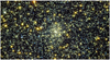 |
Fig. 1 Multiband (JHKs-combined color) infrared view of HP 1 (from the VVV survey). |
2 Data and sample
Our HP 1 CAPOS spectra are part of the 17th and final data release of SDSS-IV (Abdurro’uf et al. 2022), which includes all APOGEE-2 data. Spectra were reduced as described in Nidever et al. (2015) and analyzed using ASPCAP (García Pérez et al. 2016) and the libraries of synthetic spectra described in Zamora et al. (2015). The customised H-band line lists are fully described in Shetrone et al. (2015), Hasselquist et al. (2016), Cunha et al. (2017), and Smith et al. (2021). The APOGEE-2S plug-plates containing HP 1 members were centered on (l,b) ~ (357°, +2.0°) and (358°, +2.0°), which correspond to the APOGEE-2 programs of geisler_18a (plate name 357° +2.0°C), schlaufman_17a, and kollmeier_17a (plate name 358° +2.0°O).
We adopted the following criteria, which are based on those described in Geisler et al. (2021), Romero-Colmenares et al. (2021), and Fernández-Trincado et al. (2022c), to select our final HP 1 members: i) stars located within the tidal radius of 19 pc (30 arcmin) from the cluster center; ii) stars with proper motions (PMs) within a radius of 0.5 mas yr−1 from the mean cluster value; iii) stars with radial velocity within 20 km s−1 of the cluster mean radial velocity, 39.76 km s−1, taken from Vasiliev & Baumgardt (2021); and iv) stars differing in [Fe/H] from the assumed mean value (−1.06; Barbuy et al. 2016) by <0.3 dex. This [Fe/H] value was used as our initial metallicity, which was recalculated in this work (see Sect. 5). Fourteen stars satisfied all of these criteria and were considered our final members.
Table 1 lists the main physical parameters adopted for HP 1, while Table 2 lists the 14 members. However, we chose to analyze only the 11 stars that have a S/N >70 pixel−1. This limit for S/N has been suggested by the APOGEE team (e.g., Mészáros et al. 2020) and Fernández-Trincado et al. (2021a), 2022c) in order to guarantee reliable abundance determinations. Stars that do not meet this requirement are listed in the last three rows of Table 2. We also removed one additional star, 2M17310160–2959048, from our abundance analysis, as a visual inspection of its spectrum reveals that the Fe I lines are very weak, noisy, and with unusual line profiles, thus limiting our ability to produce reliable abundances. This star is listed in the 11th row in Table 2. We note that the ASPCAP pipeline provides some estimates of abundances for this star that we suspect are not reliable. As an initial guess, we adopted the [Fe/H] abundance ratios from ASPCAP, which are also shown in Fig. 2 and Table 3. Figure 2 summarizes the photometric, kinematic, astrometric, and metallicity properties of the 11 final HP 1 members analyzed.
Global properties of HP 1 taken from Vasiliev & Baumgardt (2021) and Harris (1996, 2010 edition).
3 Stellar parameters
The atmospheric parameters of our targets were obtained through an iterative procedure based on the Gaia (G, Bp, and Rp) and 2MASS (J, H, and KS) photometry of HP 1. During this procedure, the effective temperature (Teff) and gravity (log g) of each red giant branch (RGB) star (including our targets) were obtained, and at the same time, the color magnitude diagrams (CMDs) were corrected for differential reddening. First, we fitted a PARSEC isochrone (Bressan et al. 2012) to the RGB, assuming an age of 13.0 Gyr, as shown in Fig. 3. We accounted for reddening by applying the Cardelli et al. (1989) reddening law to the isochrone. The visual absorption, AV, the RV parameter, the intrinsic distance modulus, (m-M)0, and the global metallicity, [M/H], were determined by simultaneously fitting the red giant branch (RGB), red clump (RC), and RGB tip in the K versus Bp − K, G versus Bp − Rp, BP versus Bp − Rp, and K versus J − K CMDs. The Teff and log g of each RGB star were then determined as those corresponding to the point on the isochrone where the Ks magnitude matches that of the star (we avoided using RC stars for this step). We used the Ks magnitude because it is the least affected by reddening and, consequently, by differential reddening. Having the temperature, we obtained the intrinsic Bp − Ks color of each star from the color-temperature relation of the RGB part of the isochrone and, by subtracting the mean reddening obtained from the isochrone fitting, also the differential reddening at the position of each star. Finally, for each star we selected the four closest neighbors (five stars in total) and corrected its G, Bp, Rp, J, H, and K magnitudes using the mean differential reddening of the five stars. We used the Bp − K color because it is the most sensitive to any reddening variation. This procedure was iterated until any improvement in the CMDs was negligible.
We obtained AV = 3.8, RV = 2.4, (m−M)0 = 14.10, and [M/H] = −0.9 (dex), a value higher than the iron content of the cluster ([Fe/H] = −1.1). This is not surprising since GCs are usually α-enhanced.
The microturbulence (ξt) was determined using the empirical equation given in Dutra-Ferreira et al. (2016):
![Mathematical equation: $\[\xi_t=0.998+3.16 \times 10^{-4} X-0.253 Y-2.86 \times 10^{-4} X Y+0.165 Y^2,\]$](/articles/aa/full_html/2025/04/aa51793-24/aa51793-24-eq2.png) (1)
(1)
where X = Teff − 5500 [K] and Y = log(g) − 4.0. As Dutra-Ferreira et al. (2016) indicate, this equation is consistent with the microturbulence values computed from 3D models. We refer the reader to that paper for detailed information. Table 3 lists our derived atmospheric parameters (Teff, log g, and ξt) for the 11 HP 1 stars, and compares them to those derived from the ASPCAP pipeline.
4 Abundance determinations
We made use of the BACCHUS code (Masseron et al. 2016) to manually analyze each star in our sample, in order to examine the reliability of each atomic and molecular line present in each spectrum and derive the metallicity (from Fe I lines), broadening parameters, and chemical abundances for 12 chemical species, as listed in Table 3.
The BACCHUS code relies on the Turbospectrum radiative transfer code (Plez 2012) and the α-rich ([α/Fe] = +0.4) MARCS model atmosphere grid (Gustafsson et al. 2008), and the abundances are computed by adopting a line-by-line approach under the assumption of local thermodynamic equilibrium (LTE). For each element and each line, the abundance determination proceeds as in our previous CAPOS BACCHUS papers (Fernández-Trincado et al. 2021a). In summary, the steps are: (i) a spectrum synthesis using the full set of (atomic and molecular) lines is done to find the local continuum level via a linear fit; (ii) cosmic and telluric line rejections are performed; (iii) the local S/N per element is estimated; (iv) a series of flux points contributing to a given absorption line are automatically selected; and (v) abundances are derived by comparing the observed spectrum with a set of convolved synthetic spectra characterized by different abundances.
Four different abundance determinations are used: (i) line-profile fitting; (ii) core line-intensity comparison; (iii) equivalent-width comparison; and (iv) global goodness-of-fit estimate. Each diagnostic yields validation flags. Based on these flags, a decision tree then rejects or accepts the line, keeping the best-fit abundance. We adopted the χ2 goodness-of-fit diagnostic as the final abundance because it is considered to be the most robust. However, we stored the information from the other diagnostics, including the standard deviation between all four methods. The line list used in this work is the latest internal DR17 of atomic and molecular line list (linelist.20170418), including the s-process elements (Ce II, Nd II, and Yb II) (Hasselquist et al. 2016; Cunha et al. 2017).
In particular, a mix of heavily CN-cycled and α-rich MARCS models were used, as well as the same molecular lines adopted by APOGEE-2 (Smith et al. 2013), in order to determine the C, N, and O abundances. In addition, we adopted the C, N, and O abundances that satisfied the fitting of all molecular lines consistently; that is to say, we first derived 16O abundances from 16OH lines, then derived 12C from 12C16O lines and 14N from 12C14N lines; the C–N–O abundances were derived iteratively to minimize the 16OH, 12C16O, and 12C14N dependences (Smith et al. 2013).
The adoption of a purely photometric temperature scale enables us to be somewhat independent of the ASPCAP/APOGEE-2 pipeline, which provides important comparison data for validation. The final results presented in this paper are based on computations performed with the BACCHUS code using the photometric atmospheric parameters listed in Table 3. The same table also lists our resulting elemental abundances for the targets analyzed in this work. Figure 4 shows an example of our best BACCHUS spectral synthesis on clean selected features for star 2M17310541–2958416.
The CAPOS spectra provide access to 26 chemical species. However, most of the atomic and molecular lines are very weak and/or heavily blended, in some cases too much so to produce reliable abundances in the typical Teff, log(g), and metallicity ranges of our sample. For this reason, and after a careful visual inspection of all our spectra, we provide reliable abundance determinations for 12 selected chemical species, belonging to the iron-peak (Fe, Ni), odd-Z (Al), light (C, N), α- (O, Mg, Si, S, Ca, and Ti), and s-process (Ce) elements, which are listed in Table 3.
We did not include Na, which is often used to characterize MPs in GCs, in our analysis as this relies on two atomic lines in the H band (Na I: 1.6363 μm and 1.6388 μm) that are unfortunately too weak and too strongly blended by telluric features, and thus not able to produce reliable [Na/Fe] abundance ratios in HP 1. For this reason, in investigating MPs in HP 1, we focused on C, N, O, Mg, and Al, which are also typical chemical tracers of MPs in GCs (see, e.g., Mészáros et al. 2015; Ventura et al. 2016; Mészáros et al. 2020; Masseron et al. 2016; Pancino et al. 2017; Schiavon et al. 2017a; Fernández-Trincado et al. 2021a, 2022c; Schiavon et al. 2024).
It is important to note that two stars in our sample (2M17304363–2954441 and 2M17310585–2958354) show no reliable C12N14 lines; therefore, it was not possible to determine their [N/Fe] abundance ratios. For these particular cases, we adopted the same prescription as described in Simpson & Martell (2019) and evaluated the impact of the unknown [N/Fe] abundance ratios on [Fe/H] and [C, O/Fe], considering that carbon and oxygen abundance ratios are derived from the molecular equilibria that exist in the stellar atmosphere between C12N14, C12O16, and O16H. Thus, we assumed values of [N/Fe] ∈ {−1, −0.5, 0.0, +0.5, +1.0} and determined for each combination the corresponding [Fe/H] and [C, O/Fe] abundance ratios. The overall effect of the unknown [N/Fe] for these stars is relatively small: varying N through −1.0 < [N/Fe] < + 1.0 registers variations in Δ[C/Fe]<0.2 dex, Δ[O/Fe]<0.2 dex, and Δ[Fe/H]<0.1 dex.
For [S/Fe] abundance ratios, we find that most of the S I lines are very weak and heavily blended by other features in the typical Teff, log(g), and metallicity range of our sample, leading to unreliable [S/Fe] abundances. Therefore, the [S/Fe] abundance ratios listed in Table 3 should be taken as upper limits.
As the abundance values are sensitive to all of the atmospheric parameters, and depend on the chemical species, to estimate their uncertainties we varied the main atmospheric parameters one at a time and computed the abundances for all species for each of these possibilities for one star, 2M17305949–3000019, and calculated the typical uncertainty as σtotal, following the same methodology outlined in Fernández-Trincado et al. (2020a) and repeated in Eq. (2) for guidance. The total uncertainty, σtotal, is defined as
![Mathematical equation: $\[\sigma_{\text {total }}^2=\sigma_{[\mathrm{X} / \mathrm{H}], \mathrm{T}_{\mathrm{eff}}}^2+\sigma_{[\mathrm{X} / \mathrm{H}], \log (g)}^2+\sigma_{[\mathrm{X} / \mathrm{H}], \xi_{\mathrm{t}}}^2+\sigma_{\text {mean}}^2,\]$](/articles/aa/full_html/2025/04/aa51793-24/aa51793-24-eq3.png) (2)
(2)
where ![Mathematical equation: $\[\sigma_{\text {mean }}^{2}\]$](/articles/aa/full_html/2025/04/aa51793-24/aa51793-24-eq4.png) is calculated using the standard deviation derived from the different BACCHUS abundances of the different lines (line-by-line variation) for each element. The values of
is calculated using the standard deviation derived from the different BACCHUS abundances of the different lines (line-by-line variation) for each element. The values of ![Mathematical equation: $\[\sigma_{[X / H], T_{\mathrm{eff}}}^{2}, \sigma_{[\mathrm{X} / \mathrm{H}], \log (g)}^{2}\]$](/articles/aa/full_html/2025/04/aa51793-24/aa51793-24-eq5.png) , and
, and ![Mathematical equation: $\[\sigma_{[\mathrm{X} / \mathrm{H}], \xi_{t}}^{2}\]$](/articles/aa/full_html/2025/04/aa51793-24/aa51793-24-eq6.png) were derived for the elements in 2 M17305949–3000019 using sensitivity values of ±100 K for the temperature, ±0.3 dex for log g, and 0.05 km s−1 for the microturbulent velocity (ξt). These values were chosen as they represent the typical conservative uncertainties in the atmospheric parameters for our sample. Importantly, we note that we find lower S/Ns and/or higher S/Ns produce similar results in their uncertainties, with negligible variations in the final σtotal. Thus, the star 2M17305949–3000019 is a good representation of the HP 1 sample and it is reasonable to assume that the errors we find reflect the typical cluster star analyzed in this study. Therefore, the uncertainties listed in Table 3 for this star are considered representative of our HP 1 sample.
were derived for the elements in 2 M17305949–3000019 using sensitivity values of ±100 K for the temperature, ±0.3 dex for log g, and 0.05 km s−1 for the microturbulent velocity (ξt). These values were chosen as they represent the typical conservative uncertainties in the atmospheric parameters for our sample. Importantly, we note that we find lower S/Ns and/or higher S/Ns produce similar results in their uncertainties, with negligible variations in the final σtotal. Thus, the star 2M17305949–3000019 is a good representation of the HP 1 sample and it is reasonable to assume that the errors we find reflect the typical cluster star analyzed in this study. Therefore, the uncertainties listed in Table 3 for this star are considered representative of our HP 1 sample.
Photometry, kinematics, and astrometric properties of the 14 likely HP 1 members.
 |
Fig. 2 Main properties of HP 1 stars. Panel (a: color–magnitude diagram in the Gaia bands for cluster stars with a membership probability greater than 90% (black dots) and <90% (gray dots), taken from Vasiliev & Baumgardt (2021). The 11 stars analyzed in this work are marked with cyan symbols in all the panels. The APOGEE-2 footprint stars toward HP 1 are marked with gray dots in panels b, c, d, and e. Panel b: sky position of stars centered on HP 1; the large overlaid dashed red circle refers to the cluster tidal radius (rt). Panel c: PM distribution for stars toward the field of HP 1, with the inner zoomed window highlighting the distribution of our sample within a 0.5 mas yr−1 radius around the nominal PM of the cluster. Panel d: [Fe/H] versus the projected angular cluster distance, with the blue line showing the assumed initial mean cluster metallicity and the cyan shadow region indicating ±0.3 dex from the initial metallicity. Panel e: Radial velocity versus [Fe/H] of our member stars compared to APOGEE-2 field stars. The red box delimited by ±0.30 dex and ±20 km s−1, centered on [Fe/H] = −1.06 and RV = +39.76 km s−1, encloses our potential cluster members (see Sect. 2). The metallicity values shown in panels d and e were taken from the ASPCAP pipeline. |
BACCHUS and ASPCAP elemental abundances of ten members in HP 1.
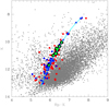 |
Fig. 3 K vs. Bp − K CMD of HP 1. The cyan line shows a portion along the RGB sequence of a 13.0 Gyr isochrone with [M/H] = −0.90 shifted using E(B–V) = 1.01 and (m-M)0 = 14.10. Gray points represent nonmember stars (according to proper motions). Red circles represent member stars, blue circles member stars corrected for differential reddening, and green circles our targets. |
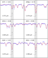 |
Fig. 4 Comparison of synthetic spectra (red lines) to the observed spectra (blue dots) for the HP 1 star 2M17310541–2958416. Each panel show the best-determined (gray shadow region) [Ti/Fe], [Mg/Fe], [Fe/H], [O/Fe], [Al/Fe], and [Si/Fe] abundance ratios listed in Table 3. An arbitrary normalized flux is plotted on the vertical axis, while the air wavelength (μm) is plotted on the horizontal axis. |
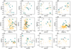 |
Fig. 5 Combined light-, odd-Z, α − and s-process elements from our BACCHUS results listed in Table 3. Panels a–1: [C/Fe]–[N/Fe], [C/Fe]–[O/Fe], [N/Fe]–[O/Fe], [N/Fe]–[Al/Fe], [Mg/Fe]–[Al/Fe], [Si/Fe]–[Al/Fe], [N/Fe]–[Mg/Fe], [Mg/Fe]–[Si/Fe], [N/Fe]–[Si/Fe], [O/Fe]–[Al/Fe], [N/Fe]–[Ce/Fe], and [Al/Fe]–[Ce/Fe] distributions for HP 1 (cyan circles), in comparison with the other APOGEE-2 GCs examined by Mészáros et al. (2020): NGC 288 (black empty squares) and NGC 5904 (orange triangles). The error bars mark the typical uncertainty (σtotal) listed in Table 3. |
5 Results and discussion
The present study adds a substantial contribution to the chemical characterization of HP 1, including detailed abundances for 12 chemical species derived from high S/N, high-resolution, near-infrared spectra of ten member giants. In the only other high-resolution spectroscopic study, Barbuy et al. (2006, 2016) analyzed a total of eight red giants in this cluster, but using optical spectra. Our sample of likely cluster members increases this number and is thus the largest sample yet analyzed spectroscopically, with the added benefit that it is based on observations in the near-infrared to help mitigate this cluster’s high reddening, allowing us to examine abundance variations within the cluster.
Figure 5 illustrates the chemical behaviors of HP 1 stars and compares them to two other GCs at similar metallicity (NGC 5904 and NGC 288) taken from Mészáros et al. (2020), whose dataset has been carefully examined with the same code and a similar methodology as adopted in this work. We avoid any comparison with GCs based only on the ASPCAP APOGEE-2 pipeline, as they can exhibit larger systematic offsets (see, e.g., Jönsson et al. 2018; Holtzman et al. 2018; Nataf et al. 2019). Thus, the listed ASPCAP values in Table 3 are only for reference and are not considered in our analysis, as our BACCHUS results are likely more precise than the ASPCAP ones.
5.1 The Fe-peak elements: Fe and Ni
We measure a mean metallicity of ⟨[Fe/H]⟩ = −1.15 ± 0.03 (standard error of the mean), with a dispersion of 0.08 ± 0.02 dex. This value is <0.1 dex more metal poor than the mean [Fe/H] = −1.06 reported by Barbuy et al. (2016), used as our initial metallicity estimate. This discrepancy is within the relative errors. Thus, we conclude that our mean [Fe/H] is in good agreement with the value reported in Barbuy et al. (2016) and that HP 1 is a cluster with an intermediate metallicity, [Fe/H] ~−1.15. We note that the mean ASPCAP value, −1.16, is very similar and also has the same dispersion. Geisler et al. (2021) derive a mean of −1.20 ± 0.10 from the ASPCAP DR16 Fe abundances for the same sample, while Geisler et al., (in prep.) find −1.23 ± 0.07 from DR 17. However, both of these values include a small negative correction to the ASPCAP metallicities of stars with high [N/Fe], which is indeed the case for most of our sample, in order to correct for ASPCAP issues for such second-generation stars. Schiavon et al. (2024) find −1.21 for a somewhat different DR17 sample and do not include a metallicity correction. Lastly, we note that the Harris (2010) catalog value for this cluster is −1, based on lower quality data. Our observed star-to-star [Fe/H] spread of 0.25 dex is quite similar to our measurement uncertainty (see Table 3), indicating that no significant metallicity variation is detected.
Regarding the other iron-peak element we examined, nickel (Ni) is on average slightly super-solar (⟨[Ni/Fe]⟩ = +0.03 ± 0.03) with a very small dispersion, <0.06 dex, and a very small star-to-star spread (~0.11 dex), within our typical uncertainties. Therefore, we do not detect a significant spread in this element either.
5.2 The odd-Z element: Al
We find that HP 1 exhibits a mean aluminum enrichment of ⟨[Al/Fe]⟩ = +0.46 ± 0.29, with a large variation in [Al/Fe], which is far beyond the typical errors. Thus, we report a strong star-to-star [Al/Fe] spread of ~0.84 dex in HP 1, which is expected for GCs at similar metallicity due to MPs (see, e.g., Pancino et al. 2017; Masseron et al. 2019; Mészáros et al. 2020).
Figures 5(e–f) reveal the strong star-to-star [Al/Fe] spread observed in HP 1, which is very similar to NGC 5904 (M 5) and NGC 288. It is clear that the extended distribution of Al is larger than the estimated errors of [Al/Fe] in HP 1 and suggests an astrophysical origin, which is likely the result of the past activation of the Mg–Al cycle nuclear fusion process at, possibly, the early stages of asymptotic giant branch (AGB) star evolution (Mészáros et al. 2015; Ventura et al. 2016). However, Figures 5(e–f; h) do not reveal any significant and clear Mg–Al/Si–Al (anti)correlations in HP 1. Similar behavior is also seen in the comparison GCs.
If the Mg–Al fusion cycle, which converts Mg into Al, is involved, it apparently does not completely process the material through the entire Mg–Al cycle, suggesting that the observed large star-to-star [Al/Fe] spread may also be due in part to diversity in the process of stellar chemical feedback and star formation in these clusters. We note that we have not been able to find any dependence of the Al abundance on effective temperature or evolutionary status (RGB or AGB), ruling out the presence of any possible analysis bias. Figure 6 reveals that the [Al/Fe] versus [Mg/Fe] abundance ratios of HP 1 stars fall clearly in the region dominated by in situ GCs, as defined by Belokurov & Kravtsov (2024), supporting our claim that HP 1 likely formed in situ, as expected for a BGC.
5.3 The α-elements: O, Mg, Si, Ca, and Ti
Table 3 reveals that HP 1 exhibits a considerable α-element enhancement, with mean values ranging from +0.20 to +0.45 ([O/Fe], [Mg/Fe], [Si/Fe], [Ca/Fe], and [Ti/Fe]), and in reasonable agreement with GCs of similar metallicity such as NGC 5904 and NGC 288, with a small star-to-star spread within our typical uncertainties, except for [O/Fe], [Si/Fe], and [Ca/Fe], which show a star-to-star spread that exceeds the observational uncertainties. [O/Fe] is the only α element with a very extended and significant spread, >0.5 dex, which is clearly (anti)correlated with light elements (C and N), as shown in Figs. 5(b–c).
It is also expected that Al is correlated with elements enhanced by proton-capture reactions (nitrogen), as demonstrated in Fig. 5(d), and anticorrelated with those depleted in H-burning at high temperatures (oxygen), as revealed in Fig. 5(j). Therefore, Al and O represent more robust indicators for the prevalence of the MP phenomenon in HP 1.
We also find a [Ca/Fe] abundance ratio scatter in HP 1, of 0.36 dex, which is larger than the typical internal uncertainties. Figure 7 reveals an intriguing correlation between [Ca/Fe] and [Al/Fe] that has not been previously seen in any bulge GC to our knowledge. The significance of this correlation is 0.74 (Pearson’s test), with a p-value of 0.05, and 0.75 (Spearman’s test) with a p-value of 0.05, suggesting the correlation is indeed significant. However, we note that the sample is small (only seven stars with measurable [Ca/Fe] abundance ratios). Moreover, two of the stars are noted to have blending issues in Al and three in Ca. Thus, more observations are needed to substantiate the reality of such a correlation. In addition, neither of our comparison GCs displays any such correlation, making our result more suspicious. Astrophysically, the Al spread is of course due to the outcome of proton-capture reactions at very high temperatures (Carretta & Bragaglia 2021). However, while a single core-collapse supernova might be enough to produce the claimed star-to-star spread in [Ca/Fe], fast-rotating massive stars (FRMSs; Decressin et al. 2007) or massive AGB stars have been proposed to produce the observed pattern in Al (Carretta et al. 2010), thus requiring multiple astrophysical processes to account for any correlation. Further research is clearly required to corroborate this intriguing possibility.
In general, we find that HP 1 exhibits average [Mg, O/Fe] abundance ratios that are in good agreement with those obtained by Barbuy et al. (2016), and which range from +0.3 ≲ [O, Mg/Fe] ≲ +0.5. Of course, the mean will depend on the MP nature of each sample, given that both of these elements are affected by MPs.
Our data yield a mean [Si/Fe] = +0.45, with some stars having enrichments as large as +0.63. The similar-sized sample analyzed by Barbuy et al. (2016) is limited to +0.15 ≲ [Si/Fe] ≲ +0.35. Indeed, our [Si/Fe] abundances appear high compared to our comparison GCs of similar metallicity in Fig. 5 as well. We note that our average [Ca/Fe] and [Ti/Fe] abundance ratios are moderately enhanced compared to those measured by Barbuy et al. (2016), who report values in the range −0.04 ≲ [Ca, Ti/Fe]≲ +0.28.
In order to validate the reliability of the observed [O/Fe] trends in HP 1, and to examine any possible bias introduced by the stellar parameters in the interpretation and discussion of our results, we applied Pearson’s and Spearman’s correlation tests to the Teff–[O/Fe] and [N/Fe]–[O/Fe] planes, and validated our results by applying a bootstrap resampling with 100 000 realizations. The Pearson’s and Spearman’s correlation coefficients range from −0.22 to −0.30 with a p-value >0.3, indicating that there is a null trend between [O/Fe] and Teff, while the Pearson’s and Spearman’s correlation coefficients range from −0.52 to −0.93 with a low p–value (<0.02), indicating that the observed [N/Fe]–[O/Fe] anticorrelation is unlikely to be due to random chance.
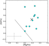 |
Fig. 6 [Mg/Fe] − [Al/Fe] distribution for HP 1 stars (cyan symbols). The black “X” symbol show the average [Mg/Fe] and [Al/Fe] abundance ratios of HP 1 from our BACCHUS values listed in Table 3. The dashed black line taken from Belokurov & Kravtsov (2024) separates the region dominated by in situ GCs (above the line) from accreted GCs (below the line). |
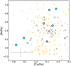 |
Fig. 7 [Ca/Fe] – [Al/Fe] distribution for HP 1 stars (cyan symbols) and our two comparison GCs. |
5.4 The light elements: C and N
HP 1 exhibits a high enrichment in nitrogen, with a mean ⟨[N/Fe]⟩ = +0.94 ± 0.43, and a large star-to-star spread of +0.95 dex, typical of MPs. HP 1 reveals a statistically significant correlation in C–O, as shown in Fig. 5(b), and clear anticorrelations in C–N (Fig. 5a) and N–O (Fig. 5c). These patterns are typical of GCs and are attributed to the prevalence of the MPs phenomenon (see e.g., Schiavon et al. 2017a, 2024, and references therein). Almost all the stars examined in HP 1 are enriched in nitrogen (except two stars with [N/Fe]< + 0.4). The chemical trends of [N/Fe] are very similar to those observed in NGC 5904 and NGC 288 (see Fig. 5), but with (at least) two groups of stars, likely compatible with a first generation ([N/Fe]≲ +0.7) and a second generation ([N/Fe]≳ +0.7; Geisler et al. 2021). This study reveals that a significant fraction of the stars with enhanced [N/Fe] abundances well above Galactic levels ([N/Fe]≳ +0.7) populate HP 1, a feature that is typical of stars in BGCs such as NGC 6380 (Fernández-Trincado et al. 2021d), and a clear indication of MPs (see e.g., Schiavon et al. 2017a; Geisler et al. 2021; Schiavon et al. 2024). Here we also report for the first time [C/Fe] abundance ratios for this cluster that are in the range −0.61 < [C/Fe] <+0.03, while Barbuy et al. (2016) report only an upper limit for [C/Fe] < 0.
The CNO trends we find are in agreement with the output of the hot CNO cycle (Wiescher et al. 2010), which predicts lower C and O and higher N abundances for the material that goes through it. However, the CNO trends we find cannot be used to discriminate between the different scenarios that have been proposed to explain the MP phenomenon and, in particular, they cannot be used to determine which polluter is responsible.
5.5 The s-process element: Ce
We find a mean ⟨[Ce/Fe]⟩ = +0.19 ± 0.03 from three stars in HP 1, which is moderately overabundant compared to the Sun and similar to the Ce levels observed in other GCs such as NGC 288 (see Fig. 5(1)). Thus, we believe that this moderate enrichment in [Ce/Fe] is likely produced by different progenitors, possibly by pollution of this cluster by low-mass AGB stars (Fernández-Trincado et al. 2021a, 2022c) after the cluster formed. Unfortunately, with only one neutron-capture element measured in HP 1 (for one of the only three stars with reliable Ce II line profiles), it is not possible to firmly determine the nucleosynthetic origins of these stars.
6 Concluding remarks
We present a detailed elemental abundance analysis using the BACCHUS package for ten stars belonging to the BGC HP 1, obtained from high S/N, high-resolution, near-IR spectra with APOGEE as part of the CAPOS survey. We examined 12 chemical species belonging to the light (C and N), α (O, Mg, Si, S, Ca, and Ti), iron-peak (Fe and Ni), odd-Z (Al), and s-process (Ce) elements. Overall, the chemical species examined so far in HP 1 are in agreement with other Galactic GCs with similar metallicities (e.g., Masseron et al. 2019; Mészáros et al. 2015; Schiavon et al. 2017a; Mészáros et al. 2020; Geisler et al. 2021; Schiavon et al. 2024). The main conclusions of this paper are the following:
HP 1 exhibits a mean ⟨[Fe/H]⟩ = −1.15 ± 0.03, with a star-to-star [Fe/H] spread, ~0.25 dex, which is quite similar to our measurement uncertainty. Thus, no significant metallicity variation is detected. Our reported average [Fe/H] is in good agreement with the metallicity estimated by Barbuy et al. (2016);
[α/Fe] ratios are enhanced, as expected, with [Si/Fe] being especially high: substantially higher than found by Barbuy et al. (2016);
The typical Mg-Al anticorrelation is not observed, which is in line with other GCs at similar metallicities (see e.g., Mészáros et al. 2020). However, a significant star-to-star [Al/Fe] spread, 0.84 dex, was identified, which (anti)correlates with [O/Fe] and [N/Fe]. We conclude that the O–Al anticorrelation and N–Al correlations represent robust indicators of the MP phenomenon in HP 1;
We find for the first time a significant variation in C, N, and O, with a clear [C/Fe]–[N/Fe] and [N/Fe]–[O/Fe] anticorrelation and [C/Fe]–[O/Fe] correlation, and a significant spread in nitrogen (>0.95 dex), carbon (>0.64 dex), and oxygen (>0.5), as expected from MPs;
HP 1 also exhibits a modest star-to-star [Ca/Fe] spread, +0.36, that exceeds the observational uncertainties. Furthermore, [Ca/Fe] correlates with [Al/Fe]. However, we note that the sample size is small and observationally limited. This finding, observed for the first time in a bulge GC, if confirmed, makes HP 1 an especially interesting representative;
Unfortunately, there are too few stars with reliable measurements of [Ce/Fe] and [S/Fe] abundance ratios to provide reliable conclusions regarding these chemical species;
HP 1 hosts a significant population of nitrogen-enriched stars, indicating the prevalence of the MP phenomenon in this cluster. Furthermore, the high nitrogen enrichment of HP 1 makes this cluster a potential progenitor of the unusual nitrogen-enhanced bulge field stars identified in the inner Galaxy, peaking at [Fe/H] ~ −1.0 (e.g., Schiavon et al. 2017b; Fernández-Trincado et al. 2022a);
The mean ⟨[Mg/Fe]⟩ = +0.29 and ⟨[Al/Fe]⟩ = +0.46 measured in this work place HP 1 in the region dominated by in situ GCs (see e.g., Belokurov & Kravtsov 2024), evidence in favor of the in situ nature of HP 1. Despite the very large scatter observed in [Al/Fe], all stars fall into the in situ domain.
In this work, we obtain one of the first detailed chemical analyses of one of the oldest in situ GCs. Further investigation, including detailed research on elements with distinct nucleosynthesis processes and comparison with a larger sample of HP 1 stars as well as similar clusters, should provide valuable insights into the unique evolutionary path of this GC in the bulge. This should contribute to our broader understanding of GC formation and evolution in the MW in general, which is the goal of the CAPOS survey. Finally, these results underscore the complex nature of chemical abundance patterns in GCs and highlight the importance of comprehensive near-infrared spectroscopic studies in unraveling the chemical signature of the MP phenomenon across the entire volume of parameter space covered by CAPOS.
Acknowledgements
The first author gratefully acknowledges the support provided by the National Agency for Research and Development (ANID)/CONICYT-PFCHA/DOCTORADO NACIONAL/2017-21171231. S.V. gratefully acknowledges the support provided by Fondecyt Regular no. 1220264, and by the ANID BASAL project ACE210002. D.G. gratefully acknowledges the support provided by Fondecyt regular no. 1220264. D.G. also acknowledges financial support from the Dirección de Investigación y Desarrollo de la Universidad de La Serena through the Programa de Incentivo a la Investigación de Académicos (PIA-DIDULS). J.G.F-T gratefully acknowledges the grants support provided by ANID Fondecyt Iniciación No. 11220340, ANID Fondecyt Postdoc No. 3230001, and from the Joint Committee ESO-Government of Chile under the agreement 2023 ORP 062/2023.
References
- Abdurro’uf, Accetta, K., Aerts, C., et al. 2022, ApJS, 259, 35 [NASA ADS] [CrossRef] [Google Scholar]
- Asplund, M., Grevesse, N., & Sauval, A. J. 2005, in Cosmic Abundances as Records of Stellar Evolution and Nucleosynthesis, eds. I. Barnes, Thomas G. & F. N. Bash, Astronomical Society of the Pacific Conference Series, 336, 25 [NASA ADS] [Google Scholar]
- Barbá, R. H., Minniti, D., Geisler, D., et al. 2019, ApJ, 870, L24 [CrossRef] [Google Scholar]
- Barbuy, B., Zoccali, M., Ortolani, S., et al. 2006, A&A, 449, 349 [NASA ADS] [CrossRef] [EDP Sciences] [Google Scholar]
- Barbuy, B., Cantelli, E., Vemado, A., et al. 2016, A&A, 591, A53 [NASA ADS] [CrossRef] [EDP Sciences] [Google Scholar]
- Bastian, N., & Lardo, C. 2018, ARA&A, 56, 83 [Google Scholar]
- Bastian, N., Lamers, H. J. G. L. M., de Mink, S. E., et al. 2013, MNRAS, 436, 2398 [CrossRef] [Google Scholar]
- Belokurov, V., & Kravtsov, A. 2024, MNRAS, 528, 3198 [CrossRef] [Google Scholar]
- Bica, E., Ortolani, S., & Barbuy, B. 2016, PASA, 33, e028 [Google Scholar]
- Bica, E., Ortolani, S., Barbuy, B., & Oliveira, R. A. P. 2024, A&A, 687, A201 [NASA ADS] [CrossRef] [EDP Sciences] [Google Scholar]
- Blanton, M. R., Bershady, M. A., Abolfathi, B., et al. 2017, AJ, 154, 28 [Google Scholar]
- Bowen, I. S., & Vaughan, A. H. J., 1973, Appl. Opt., 12, 1430 [Google Scholar]
- Bressan, A., Marigo, P., Girardi, L., et al. 2012, MNRAS, 427, 127 [NASA ADS] [CrossRef] [Google Scholar]
- Cardelli, J. A., Clayton, G. C., & Mathis, J. S. 1989, ApJ, 345, 245 [Google Scholar]
- Carretta, E., & Bragaglia, A. 2021, A&A, 646, A9 [EDP Sciences] [Google Scholar]
- Carretta, E., Bragaglia, A., Gratton, R. G., et al. 2009, A&A, 505, 117 [NASA ADS] [CrossRef] [EDP Sciences] [Google Scholar]
- Carretta, E., Bragaglia, A., Gratton, R., et al. 2010, ApJ, 712, L21 [NASA ADS] [CrossRef] [Google Scholar]
- Cunha, K., Smith, V. V., Hasselquist, S., et al. 2017, ApJ, 844, 145 [Google Scholar]
- D’Antona, F., Vesperini, E., D’Ercole, A., et al. 2016, MNRAS, 458, 2122 [Google Scholar]
- de Mink, S. E., Pols, O. R., Langer, N., & Izzard, R. G. 2009, A&A, 507, L1 [NASA ADS] [CrossRef] [EDP Sciences] [Google Scholar]
- Decressin, T., Meynet, G., Charbonnel, C., Prantzos, N., & Ekström, S. 2007, A&A, 464, 1029 [NASA ADS] [CrossRef] [EDP Sciences] [Google Scholar]
- Dutra-Ferreira, L., Pasquini, L., Smiljanic, R., Porto de Mello, G. F., & Steffen, M. 2016, A&A, 585, A75 [NASA ADS] [CrossRef] [EDP Sciences] [Google Scholar]
- Fernández-Trincado, J. G., Zamora, O., Souto, D., et al. 2019, A&A, 627, A178 [Google Scholar]
- Fernández-Trincado, J. G., Beers, T. C., & Minniti, D. 2020a, A&A, 644, A83 [Google Scholar]
- Fernández-Trincado, J. G., Minniti, D., Beers, T. C., et al. 2020b, A&A, 643, A145 [Google Scholar]
- Fernández-Trincado, J. G., Beers, T. C., Barbuy, B., et al. 2021a, ApJ, 918, L9 [CrossRef] [Google Scholar]
- Fernández-Trincado, J. G., Beers, T. C., Minniti, D., et al. 2021b, A&A, 647, A64 [EDP Sciences] [Google Scholar]
- Fernández-Trincado, J. G., Beers, T. C., Minniti, D., et al. 2021c, A&A, 648, A70 [Google Scholar]
- Fernández-Trincado, J. G., Minniti, D., Souza, S. O., et al. 2021d, ApJ, 908, L42 [Google Scholar]
- Fernández-Trincado, J. G., Beers, T. C., Barbuy, B., et al. 2022a, A&A, 663, A126 [NASA ADS] [CrossRef] [EDP Sciences] [Google Scholar]
- Fernández-Trincado, J. G., Minniti, D., Garro, E. R., & Villanova, S. 2022b, A&A, 657, A84 [NASA ADS] [CrossRef] [EDP Sciences] [Google Scholar]
- Fernández-Trincado, J. G., Villanova, S., Geisler, D., et al. 2022c, A&A, 658, A116 [NASA ADS] [CrossRef] [EDP Sciences] [Google Scholar]
- García Pérez, A. E., Allende Prieto, C., Holtzman, J. A., et al. 2016, AJ, 151, 144 [Google Scholar]
- Geisler, D., Villanova, S., O’Connell, J. E., et al. 2021, A&A, 652, A157 [NASA ADS] [CrossRef] [EDP Sciences] [Google Scholar]
- González-Díaz, D., Fernández-Trincado, J. G., Villanova, S., et al. 2023, MNRAS, 526, 6274 [CrossRef] [Google Scholar]
- Grevesse, N., Scott, P., Asplund, M., & Sauval, A. J. 2015, A&A, 573, A27 [CrossRef] [EDP Sciences] [Google Scholar]
- Gustafsson, B., Edvardsson, B., Eriksson, K., et al. 2008, A&A, 486, 951 [NASA ADS] [CrossRef] [EDP Sciences] [Google Scholar]
- Harris, W. E. 1996, AJ, 112, 1487 [Google Scholar]
- Harris, W. E. 2010, arXiv e-prints [arXiv:1012.3224] [Google Scholar]
- Hasselquist, S., Shetrone, M., Cunha, K., et al. 2016, ApJ, 833, 81 [Google Scholar]
- Holtzman, J. A., Hasselquist, S., Shetrone, M., et al. 2018, AJ, 156, 125 [Google Scholar]
- Jönsson, H., Allen de Prieto, C., Holtzman, J. A., et al. 2018, AJ, 156, 126 [CrossRef] [Google Scholar]
- Kerber, L. O., Libralato, M., Souza, S. O., et al. 2019, MNRAS, 484, 5530 [Google Scholar]
- Majewski, S. R., Schiavon, R. P., Frinchaboy, P. M., et al. 2017, AJ, 154, 94 [NASA ADS] [CrossRef] [Google Scholar]
- Massari, D., Koppelman, H. H., & Helmi, A. 2019, A&A, 630, L4 [NASA ADS] [CrossRef] [EDP Sciences] [Google Scholar]
- Masseron, T., García-Hernández, D. A., Mészáros, S., et al. 2019, A&A, 622, A191 [NASA ADS] [CrossRef] [EDP Sciences] [Google Scholar]
- Masseron, T., Merle, T., & Hawkins, K. 2016, BACCHUS: Brussels Automatic Code for Characterizing High accUracy Spectra, Astrophysics Source Code Library [record ascl:1605.004] [Google Scholar]
- Mészáros, S., Martell, S. L., Shetrone, M., et al. 2015, AJ, 149, 153 [Google Scholar]
- Mészáros, S., Masseron, T., García-Hernández, D. A., et al. 2020, MNRAS, 492, 1641 [Google Scholar]
- Mészáros, S., Masseron, T., Fernández-Trincado, J. G., et al. 2021, MNRAS, 505, 1645 [Google Scholar]
- Minniti, D. 1995, AJ, 109, 1663 [NASA ADS] [CrossRef] [Google Scholar]
- Minniti, D., Alonso-García, J., Braga, V., et al. 2017a, RNAAS, 1, 16 [Google Scholar]
- Minniti, D., Geisler, D., Alonso-García, J., et al. 2017b, ApJ, 849, L24 [CrossRef] [Google Scholar]
- Nataf, D. M., Wyse, R. F. G., Schiavon, R. P., et al. 2019, AJ, 158, 14 [Google Scholar]
- Nidever, D. L., Holtzman, J. A., Allende Prieto, C., et al. 2015, AJ, 150, 173 [NASA ADS] [CrossRef] [Google Scholar]
- Palma, T., Minniti, D., Alonso-García, J., et al. 2019, MNRAS, 487, 3140 [Google Scholar]
- Pancino, E., Romano, D., Tang, B., et al. 2017, A&A, 601, A112 [NASA ADS] [CrossRef] [EDP Sciences] [Google Scholar]
- Plez, B. 2012, Turbospectrum: Code for spectral synthesis, Astrophysics Source Code Library [record ascl:1205.004] [Google Scholar]
- Renzini, A., D’Antona, F., Cassisi, S., et al. 2015, MNRAS, 454, 4197 [Google Scholar]
- Romero-Colmenares, M., Fernández-Trincado, J. G., Geisler, D., et al. 2021, A&A, 652, A158 [NASA ADS] [CrossRef] [EDP Sciences] [Google Scholar]
- Saito, R. K., Hempel, M., Minniti, D., et al. 2012, A&A, 537, A107 [NASA ADS] [CrossRef] [EDP Sciences] [Google Scholar]
- Schiavon, R. P., Johnson, J. A., Frinchaboy, P. M., et al. 2017a, MNRAS, 466, 1010 [NASA ADS] [CrossRef] [Google Scholar]
- Schiavon, R. P., Phillips, S. G., Myers, N., et al. 2024, MNRAS, 528, 1393 [CrossRef] [Google Scholar]
- Schiavon, R. P., Zamora, O., Carrera, R., et al. 2017b, MNRAS, 465, 501 [Google Scholar]
- Shetrone, M., Bizyaev, D., Lawler, J. E., et al. 2015, ApJS, 221, 24 [Google Scholar]
- Simpson, J. D., & Martell, S. L. 2019, MNRAS, 490, 741 [NASA ADS] [CrossRef] [Google Scholar]
- Smith, V. V., Cunha, K., Shetrone, M. D., et al. 2013, ApJ, 765, 16 [Google Scholar]
- Smith, V. V., Bizyaev, D., Cunha, K., et al. 2021, AJ, 161, 254 [NASA ADS] [CrossRef] [Google Scholar]
- Vasiliev, E., & Baumgardt, H. 2021, MNRAS, 505, 5978 [NASA ADS] [CrossRef] [Google Scholar]
- Ventura, P., García-Hernández, D. A., Dell’Agli, F., et al. 2016, ApJ, 831, L17 [Google Scholar]
- Wiescher, M., Görres, J., Uberseder, E., Imbriani, G., & Pignatari, M. 2010, Annual Review of Nuclear and Particle Science, 60, 381 [NASA ADS] [CrossRef] [Google Scholar]
- Zamora, O., García-Hernández, D. A., Allende Prieto, C., et al. 2015, AJ, 149, 181 [CrossRef] [Google Scholar]
All Tables
Global properties of HP 1 taken from Vasiliev & Baumgardt (2021) and Harris (1996, 2010 edition).
Photometry, kinematics, and astrometric properties of the 14 likely HP 1 members.
All Figures
|
Fig. 1 Multiband (JHKs-combined color) infrared view of HP 1 (from the VVV survey). |
| In the text | |
|
Fig. 2 Main properties of HP 1 stars. Panel (a: color–magnitude diagram in the Gaia bands for cluster stars with a membership probability greater than 90% (black dots) and <90% (gray dots), taken from Vasiliev & Baumgardt (2021). The 11 stars analyzed in this work are marked with cyan symbols in all the panels. The APOGEE-2 footprint stars toward HP 1 are marked with gray dots in panels b, c, d, and e. Panel b: sky position of stars centered on HP 1; the large overlaid dashed red circle refers to the cluster tidal radius (rt). Panel c: PM distribution for stars toward the field of HP 1, with the inner zoomed window highlighting the distribution of our sample within a 0.5 mas yr−1 radius around the nominal PM of the cluster. Panel d: [Fe/H] versus the projected angular cluster distance, with the blue line showing the assumed initial mean cluster metallicity and the cyan shadow region indicating ±0.3 dex from the initial metallicity. Panel e: Radial velocity versus [Fe/H] of our member stars compared to APOGEE-2 field stars. The red box delimited by ±0.30 dex and ±20 km s−1, centered on [Fe/H] = −1.06 and RV = +39.76 km s−1, encloses our potential cluster members (see Sect. 2). The metallicity values shown in panels d and e were taken from the ASPCAP pipeline. |
| In the text | |
|
Fig. 3 K vs. Bp − K CMD of HP 1. The cyan line shows a portion along the RGB sequence of a 13.0 Gyr isochrone with [M/H] = −0.90 shifted using E(B–V) = 1.01 and (m-M)0 = 14.10. Gray points represent nonmember stars (according to proper motions). Red circles represent member stars, blue circles member stars corrected for differential reddening, and green circles our targets. |
| In the text | |
|
Fig. 4 Comparison of synthetic spectra (red lines) to the observed spectra (blue dots) for the HP 1 star 2M17310541–2958416. Each panel show the best-determined (gray shadow region) [Ti/Fe], [Mg/Fe], [Fe/H], [O/Fe], [Al/Fe], and [Si/Fe] abundance ratios listed in Table 3. An arbitrary normalized flux is plotted on the vertical axis, while the air wavelength (μm) is plotted on the horizontal axis. |
| In the text | |
|
Fig. 5 Combined light-, odd-Z, α − and s-process elements from our BACCHUS results listed in Table 3. Panels a–1: [C/Fe]–[N/Fe], [C/Fe]–[O/Fe], [N/Fe]–[O/Fe], [N/Fe]–[Al/Fe], [Mg/Fe]–[Al/Fe], [Si/Fe]–[Al/Fe], [N/Fe]–[Mg/Fe], [Mg/Fe]–[Si/Fe], [N/Fe]–[Si/Fe], [O/Fe]–[Al/Fe], [N/Fe]–[Ce/Fe], and [Al/Fe]–[Ce/Fe] distributions for HP 1 (cyan circles), in comparison with the other APOGEE-2 GCs examined by Mészáros et al. (2020): NGC 288 (black empty squares) and NGC 5904 (orange triangles). The error bars mark the typical uncertainty (σtotal) listed in Table 3. |
| In the text | |
|
Fig. 6 [Mg/Fe] − [Al/Fe] distribution for HP 1 stars (cyan symbols). The black “X” symbol show the average [Mg/Fe] and [Al/Fe] abundance ratios of HP 1 from our BACCHUS values listed in Table 3. The dashed black line taken from Belokurov & Kravtsov (2024) separates the region dominated by in situ GCs (above the line) from accreted GCs (below the line). |
| In the text | |
|
Fig. 7 [Ca/Fe] – [Al/Fe] distribution for HP 1 stars (cyan symbols) and our two comparison GCs. |
| In the text | |
Current usage metrics show cumulative count of Article Views (full-text article views including HTML views, PDF and ePub downloads, according to the available data) and Abstracts Views on Vision4Press platform.
Data correspond to usage on the plateform after 2015. The current usage metrics is available 48-96 hours after online publication and is updated daily on week days.
Initial download of the metrics may take a while.