| Issue |
A&A
Volume 694, February 2025
|
|
|---|---|---|
| Article Number | A121 | |
| Number of page(s) | 13 | |
| Section | Extragalactic astronomy | |
| DOI | https://doi.org/10.1051/0004-6361/202451403 | |
| Published online | 11 February 2025 | |
Overdensity of Lyman-break galaxy candidates around hot-dust-obscured galaxies
1
Instituto de Estudios Astrofísicos, Facultad de Ingeniería y Ciencias, Universidad Diego Portales, Av. Ejército Libertador 441, Santiago, Chile
2
Centre for Space Research, North-West University, Potchefstroom 2520, South Africa
3
ICRAR, The University of Western Australia, 35 Stirling Highway, Crawley, WA 6009, Australia
4
Instituto de Astrofísica, Facultad de Física, Pontificia Universidad Católica de Chile, Santiago 7820436, Chile
5
Las Campanas Observatory, Carnegie Institution of Washington, Raúl Bitrán 1200, La Serena, Chile
6
Department of Physics, Northwestern College, 101 7th St SW, Orange City, IA 51041, USA
7
School of Physics, Korea Institute for Advanced Study, 85 Hoegiro, Dongdaemun-gu, Seoul 02455, Republic of Korea
8
National Astronomical Observatories, Chinese Academy of Sciences, 20A Datun Road, Beijing 100101, China
9
Institute for Frontiers in Astronomy and Astrophysics, Beijing Normal University Beijing 102206, China
10
University of Chinese Academy of Sciences, Beijing 100049, China
11
Jet Propulsion Laboratory, California Institute of Technology, 4800 Oak Grove Drive, Pasadena, CA 91109, USA
12
Department of Physics, University of Crete, 70013 Heraklion, Greece
13
Institute of Astrophysics, Foundation for Research and Technology–Hellas (FORTH), Heraklion GR-70013, Greece
14
School of Sciences, European University Cyprus, Diogenes street, Engomi, 1516 Nicosia, Cyprus
15
IPAC, California Institute of Technology, 1200 E. California Boulevard, Pasadena, 91125 CA, USA
16
Physics & Astronomy, University of Leicester, 1 University Road, Leicester LE1 7RH, UK
⋆ Corresponding author; dejene.woldeyes@mail.udp.cl
Received:
6
July
2024
Accepted:
4
December
2024
Hot dust-obscured galaxies (hot DOGs) are a family of hyper-luminous, heavily obscured quasars. A number of studies based on the identification of companions at optical to far-infrared (FIR) wavelengths have shown that these objects reside in significantly overdense regions of the Universe. Here we present further characterisation of their environments by studying the surface density of Lyman break galaxy (LBG) candidates in the vicinity of three hot DOGs. For two of them, WISE J041010.60–091305.2 (W0410–0913) at z = 3.631 and WISE J083153.25+014010.8 (W0831+0140) at z = 3.912, we identify the candidate LBG companions using deep observations obtained with Baade/IMACS. For the third, WISE J224607.56–052634.9 (W2246–0526) at z = 4.601, we reanalyse previously published data obtained with Gemini-S/GMOS-S. We optimise the LBG photometric selection criteria at the redshift of each target using the COSMOS2020 catalog. When comparing the density of LBG candidates found in the vicinity of these hot DOGs with that in the COSMOS2020 catalog, we find overdensities of δ = 1.83 ± 0.08 (δ′ = 7.49 ± 0.68), δ = 4.67 ± 0.21 (δ′ = 29.17 ± 2.21), and δ = 2.36 ± 0.25 (δ′ = 11.60 ± 1.96) around W0410–0913, W0831+0140, and W2246–0526, respectively, without (with) contamination correction. Additionally, we find that the overdensities are centrally concentrated around each hot DOG. Our analysis also reveals that the overdensity of the fields surrounding W0410–0913 and W0831+0140 declines steeply beyond physical scales of ∼2 Mpc. If these overdensities evolve into clusters by z = 0, the present results suggest that the hot DOG may correspond to the early formation stages of the brightest cluster galaxy. We were unable to determine whether or not this is also the case for W2246–0526 due to the smaller field of view (FOV) of the GMOS-S observations. Our results imply that hot DOGs may be excellent tracers of protoclusters.
Key words: galaxies: evolution / galaxies: formation / galaxies: high-redshift / galaxies: structure
© The Authors 2025
 Open Access article, published by EDP Sciences, under the terms of the Creative Commons Attribution License (https://creativecommons.org/licenses/by/4.0), which permits unrestricted use, distribution, and reproduction in any medium, provided the original work is properly cited.
This article is published in open access under the Subscribe to Open model. Subscribe to A&A to support open access publication.
1. Introduction
The hierarchical assembly of galaxies implies that the environment in which galaxies are born and live can play a fundamental role in driving their evolution (e.g. Li et al. 2007; Dayal et al. 2019). This merging process may trigger active galactic nuclei (AGNs) activity, driving the growth of the supermassive black holes (SMBHs) at their centers. As we know that SMBHs assemble the majority of their mass through gas accretion during AGN phases (Soltan 1982; Inayoshi et al. 2020), it is likely that the most luminous quasars live in overdense regions of the Universe. In particular, the existence of SMBHs with > 108−9 M⊙ in the early Universe (z ≳ 6; e.g. Bañados et al. 2018; Wang et al. 2021; Fan et al. 2023, for a recent review) implies that these sources must be fed by large amounts of gas, and that they must live in the densest regions at that time (Overzier et al. 2009; Angulo et al. 2012). However, the observational evidence appears controversial.
Spanning over two decades, the exploration of overdensities around luminous high-redshift quasars and radio galaxies has notably deepened our comprehension of their environment throughout cosmic time (e.g. Zheng et al. 2006; Kim et al. 2009; Utsumi et al. 2010; Husband et al. 2013; Morselli et al. 2014; García-Vergara et al. 2017, 2019; Mazzucchelli et al. 2017; Uchiyama et al. 2018; Mignoli et al. 2020; Lambert et al. 2024). Spectroscopically identifying companion galaxies around quasars and radio galaxies is difficult due to the inherent faintness of the surrounding galaxies, and so various methods based purely on photometric observations have been devised to trace overdense regions. The most common of these include identification of either Lyman-break galaxies (LBGs; e.g. Steidel et al. 2003; Ouchi et al. 2004; Yoshida et al. 2006; Husband et al. 2013; Morselli et al. 2014; García-Vergara et al. 2017) through broad-band optical colours, or Lyman-alpha emitters (LAEs, e.g. Kashikawa et al. 2007; García-Vergara et al. 2019) via a combination of broad- and narrow-band observations.
Some studies find overdensities around high-redshift radio galaxies (1 < z < 5; e.g. Venemans et al. 2002, 2004, 2007; Miley et al. 2004; Intema et al. 2006; Mayo et al. 2012; Bosman et al. 2020) and high-redshift quasars (z ≳ 4; e.g. Zheng et al. 2006; Morselli et al. 2014; Balmaverde et al. 2017; García-Vergara et al. 2017). Others find a mix of overdensity and underdensity of LBGs (z ≥ 6; e.g. Kim et al. 2009; Ota et al. 2018; Champagne et al. 2023). There are also studies that find no overdensity of LAEs/LBGs around high-redshift quasars (z > 5.5; e.g. Bañados et al. 2013; Mazzucchelli et al. 2017; Uchiyama et al. 2018). Recently, Lambert et al. (2024) found evidence that the quasar itself may hinder star formation in its vicinity, suggesting that using LAEs as overdensity tracers should be done with caution. Despite these potential caveats, overdense environments provide a unique opportunity to understand the formation of large-scale structures, such as protoclusters in the early Universe.
Hot dust-obscured galaxies (hot DOGs; Eisenhardt et al. 2012; Wu et al. 2012), discovered through the Wide-field Infrared Survey Explorer (WISE; Wright et al. 2010) mission, are among some of the most luminous and rare populations of quasars. These objects are powered by intense accretion onto SMBHs, which are heavily buried under enormous amounts of gas and dust (Stern et al. 2014; Tsai et al. 2015, 2018; Assef et al. 2015). Recently, Li et al. (2024) estimated the black hole masses of hot DOGs using the broad CIV and MgII lines and found that they range from 108.7 to 1010 M⊙. Hot DOGs have extreme bolometric luminosities, Lbol > 1013 L⊙, with some exceeding Lbol > 1014 L⊙ (Tsai et al. 2015). These objects may play a significant role in the evolution of their host galaxies by inducing substantial gas outflows (Díaz-Santos et al. 2016; Jun et al. 2020; Finnerty et al. 2020).
Previous studies of the environments of hot DOGs have found that they inhabit densely populated regions (Jones et al. 2014, 2017; Assef et al. 2015; Fan et al. 2017; Zewdie et al. 2023). In particular, Assef et al. (2015) studied a large number of hot DOGs through Spitzer/IRAC imaging and statistically revealed that these objects exist in dense environments similar to those hosting radio-loud AGN (e.g. Wylezalek et al. 2013; Noirot et al. 2018). Jones et al. (2014, 2017) explored the overdensities of submillimeter galaxies (SMGs) and mid-infrared (MIR) Spitzer-selected galaxies situated in proximity to hot DOGs. Their findings also suggest that hot DOGs could potentially reside in overdense environments.
Ginolfi et al. (2022) studied the environment of WISE J041010.60–091305.2 (W0410–0913, z = 3.361) using VLT/MUSE observations and found a significant overdensity of LAEs around this hot DOG ( , where
  , NF is the number of LAE/LBG candidates in the targeted field, and NE is the number of LAEs/LBGs in the blank field normalised to the area of the targeted field). Luo et al. (2022) found double the surface density of distant red galaxies around W1835+4355 at z = 2.3 compared to the field. Recently, Zewdie et al. (Zewdie et al., hereafter 2023Zewdie) studied the environment of the most luminous known hot DOG WISE J224607.56–052634.9 (W2246–0526) at z = 4.601 using deep Gemini Multi-Object Spectrographs South (GMOS-S) imaging in the r, i, and z bands. These authors revealed a large overdensity (δ ∼ 6) of LBGs within 1.4 Mpc of the hot DOG, suggesting it lives in an early-stage protocluster. However, they did not observe a radial profile overdensity of LBGs around the hot DOG. They interpreted this as implying that either the hot DOG is not at the centre, that the structure is too young to have a clear centre even if the hot DOG becomes the brightest cluster galaxy (BCG), or that observational effects from the selection cancel out the radial profile. Further indications of the overdense environment around this source have also been found by deep ALMA observations: Díaz-Santos et al. (2016, 2018) revealed the presence of companions around W2246–0526 linked by dust streams up to 30 kpc from the hot DOG. Their findings suggest that this system is a triple merger, in a locally dense environment.
In the present work, we study the environment of three hot DOGs, namely W0410–0913, WISE J083153.25+014010.8 (W0831+0140), and W2246–0526, through the identification of LBG companions. We use optimised selection functions based on the observations, redshifts, and classifications of the Cosmic Evolution Survey (COSMOS; Scoville et al. 2007; Weaver et al. 2022) catalogue. Specifically, we investigate LBG candidates around W0410–0913 (z = 3.631) and W0831+0140 (z = 3.912) selected as g-band dropouts in imaging obtained with the Inamori-Magellan Areal Camera and Spectrograph (IMACS) at the Magellan Baade Telescope. Additionally, we reanalyse the data from 2023Zewdie for W2246–0526 using the same technique to optimise the selection function as that used for the other two fields. This paper is organised as follows: In Section 2, we discuss our IMACS observations, data reduction, photometric measurements, and the COSMOS2020 catalogue. In Section 3, we present the optimisation of the selection function based on the colour selection criteria. In Section 4, we discuss the study of the colour and spatial distribution of the LBG candidates and we compare our results with those for other hot DOG and quasar environments presented in the literature. Our conclusions are presented in Section 5. Throughout this paper, all magnitudes are given in the AB system. We assume a flat ΛCDM cosmology with H0 = 70 km s−1 Mpc−1 and ΩM = 0.3.
2. Observations and data reduction
2.1. Magellan/IMACS observations
We used the IMACS instrument with the f/4 camera on the Magellan Baade telescope to obtain deep images in the g, r, and i bands of the fields around W0410–0913 and W0831+0140 on the night of 25 November 2019 (P.I.: R.J. Assef). The average seeing was 1.02″, 1.07″, and 1.08″ for the W0410–0913 observations in the g, r, and i bands, respectively, with airmass ranging from 1.07 to 1.15. For the W0831+0140 observations, the mean seeing was 0.81″, 1.10″, and 1.01″ in the r, g, and i bands, respectively, with the airmass ranging from 1.17 to 1.54. All images have a pixel scale of 0.22″ pix−1 and a field of view (FOV) of 15.4′× 15.4′. A dithering pattern with offsets of between 20″ and 60″ in right ascension (RA) and declination (Dec) was applied to minimise the effect of the chip gaps in the final stacked image. The details of the observations are summarised in Table 1.
Summary of IMACS and GMOS-S observations used in this work. All data were acquired during the night of 25 November 2019 for both IMACS observations and nights of 16/23/27 September 2017 for W2246–0526 GMOS-S observations (2023Zewdie).
2.2. IMACS data reduction
We reduced the IMACS observations by first applying bias and flat-field corrections using Theli1 (Erben et al. 2005; Schirmer 2013). The raw IMACS images do not come with World Coordinate System (WCS) information, and so we developed a python package2 to calibrate the image astrometry. We first made an initial guess based on the telescope information in the image headers. We then cross-matched sources in our images with objects in Gaia DR3 (Gaia Collaboration 2023) using the astroquery package. The pixel-to-world relation was then used to define an accurate WCS object for each image. We found that the initial guess was inaccurate by about 20″. Finally, we used Swarp3 to co-add our images (Bertin et al. 2002).
There are a number of saturated stars, particularly in the field of W0410–0913, with large saturation spikes that cause irregular systematic features in the image, and so we applied some conservative masking to avoid the detection of spurious sources near the saturated spikes. The final masked images are shown in Figure 1. We estimated the usable area by generating 106 random points distributed throughout the image and counted the fraction of unmasked points. The usable area remaining after masking is ∼212.6 arcmin2 and ∼235.7 arcmin2 for the W0410–0913 and W0831+0140 fields, respectively. The IMACS instrument is composed of eight CCDs with a gap between them at the centre of the FOV. Therefore, we centred the targets on one of the CCDs. We considered the region around the hot DOG as the centre up to a maximum radius. We refer to this area as the ‘inner region’, which has a radius of ∼4.8′.
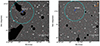 |
Fig. 1. r-band image of W0410–0913 (left-panel) and W0831+0140 (right-panel). In both panels, black circles and polygons show the masked area that we did not use for our LBG selection (see Section 2.1 for details). The blue circles and arrows indicate the hot DOGs positions, and the cyan circle represents the largest area centred on the hot DOG within the image bounds. The red circles are candidate LBG companions. |
2.3. Photometry
We measured the photometry using fixed apertures of 2″ diameter with SExtractor4 (Bertin & Arnouts 1996) in dual-image mode, using the r-band images for source detection. We used detection and analysis thresholds of 3 pixels detected above 1.5σ. We applied a 5 × 5 convolution filter based on a Gaussian point spread function (PSF) with a full width at half maximum (FWHM) of 3.0 pix (0.66″). For the background, we used a global model with mesh and filter sizes of 32 and 3 in pixels, respectively.
Photometric calibration was conducted using data from the Panoramic Survey Telescope & Rapid Response System (PanSTARRS) Survey (Tonry et al. 2012). We exclusively considered point sources, which were selected based on the probabilistic classification of unresolved point sources with a ps_score of greater than 0.83, following the suggestion by Tachibana & Miller (2018)5. The PanSTARRS point sources were cross-matched with our sources using a 1″ radius, resulting in 175 and 372 matches within the unmasked areas of the W0410–0913 and W0831+0140 fields, respectively. To address potential issues with saturation and non-linearity in the IMACS images, as well as issues with low-signal-to-noise-ratio (S/N) detections in PanSTARRS, we only considered PanSTARRS point sources within the PSF magnitude ranges of 18.0 < g < 22.5, 17.5 < r < 21.5, and 17.0 < i < 21.0, resulting in 71 (201), 78 (205), and 77 (204) sources, respectively, for W0410–0913 (W0831+0140). To calibrate the IMACS g-band observations, we found that a single colour term, g − r from PanSTARRS, was needed in addition to the PanSTARRS g-band magnitude. For the IMACS r band, we found that two colour terms were needed, and so we used the g − r and r − i PanSTARRS colours. Similarly, for the IMACS i band, we found that we needed to use the r − i and i − z PanSTARRS colours. The 1, 3, and 5σ depths of the image stacks are presented in Table 1.
We also used deep GMOS imaging data in the r, i, and z bands of Gemini GMOS-S presented by 2023Zewdie in the field around W2246–0526. The magnitude limits of the stacked images for the 5σ, 3σ, and 1σ depths of the i and z bands are detailed in Table 1. Using a similar criteria for masking as was done for the IMACS observations resulted in a final FoV of 23.7 arcmin2 as shown in Figure 2. For further details, we refer the reader to 2023Zewdie.
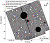 |
Fig. 2. i-band image of W2246–0526. The solid orange circle indicates the position of this hot DOG. The blue circles show the LBG candidates selected by 2023Zewdie using the modified selection criteria and with optimised selection criteria. The black circles and rectangles show the masked area. The red circles and rectangles show the LBG candidates only selected by 2023Zewdie and using optimised selection criteria, respectively. Figure adapted from 2023Zewdie. |
3. Optimisation of the LBG selection function
3.1. COSMOS data
The COSMOS2020 field offers a unique multiwavelength dataset covering a relatively large area of ∼2 deg2. Here, we use the COSMOS2020 CLASSIC catalogue (Weaver et al. 2022)6, where source detection was conducted using SExtractor. The catalogue provides observations in multiple broad and medium photometric bands. Additionally, it provides spectroscopic and photometric redshift estimates obtained with LePhare (Arnouts et al. 2002; Ilbert et al. 2006) and EAZY (Brammer et al. 2008) for more than 1.7 million sources. Weaver et al. (2022) quantify the uncertainty in photometric redshift estimates using the normalised median absolute deviation (NMAD; Hoaglin et al. 1983), defined as  . In COSMOS2020, the precision of photometric redshifts (expressed as σNMAD) is typically subpercent, that is, about 0.01(1 + z) for sources with i < 21. For the faintest sources (25 < i < 27), the precision remains around 5%, and stays better than 0.025(1 + z) for sources with i < 25.
In this work, we use the photometry and photometric redshift estimates in the COSMOS2020 catalogue to optimise the LBG selection function for each of the hot DOG fields studied, as discussed in the following section. We specifically use the Subaru HSC photometry in the g, r, i, and z bands, which have 3σ depths of 28.1, 27.8, 27.6, and 27.2 mag, respectively, within 2″ apertures. We only considered sources whose photometry is not affected by saturated stars and their spikes. We further require sources to be in the overlap region of the UltraVISTA, HSC, and SuprimeCam imaging (i.e. FLAG_COMBINED, clean = 0; hereafter, combined catalog, see Weaver et al. 2022) to ensure a uniform quality of photometric redshifts and object classifications. The area of this combined region is 1.278 deg2. The combined COSMOS2020 catalogue has a total of 723 897 sources and includes spectroscopic or accurate photometric redshift estimates, as well as separate classifications for galaxies (711 918), stars (9644), X-rays sources (2170), and failure sources (165), which enable us to estimate the contamination level. As shown in Figure 3, the filter curves are very similar between the instruments. Hence, it is not required to calculate the colour differences between them.
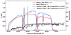 |
Fig. 3. Composite LBG spectrum from Shapley et al. (2003) shifted to z = 3.631 (black dashed lines) and z = 3.912 (grey solid lines), used for optimising the selection function for the W0410–0913 and W0831+0140 fields, respectively. After accounting for quantum efficiency and atmospheric transmission, the red and blue lines represent the HSC filter curves (used for optimisation and the blank field) and the IMACS filter curves (used for W0410–0913 and W0831+0140), respectively. |
3.2. LBG selection function
LBGs are actively star-forming galaxies and, as such, have intrinsically blue spectral energy distributions (SEDs) in the rest-frame UV down to the wavelength of the Lyα emission line. At wavelengths shorter than this, their SEDs are significantly depressed by intergalactic Lyα absorption and by the Lyman break shortward of 912 Å. Photometric identification of LBGs is typically done using three photometric bands. The colour between the two bluest bands is used to identify the drop in flux due to the Lyman break, while the colour between the two redder bands maps the rest-frame UV continuum of the galaxy.
For the two lower-redshift targets, W0410–0913 and W0831+0140, we identify companion galaxies using g − r and r − i colours, while for W2246–0526 we use r − i and i − z colours instead. The exact colour limits one uses determines the purity and the completeness of the LBG sample. In order to optimise the selection function, we used the redshift estimates and the HSC g, r, i, and z photometry of COSMOS2020 sources in the combined COSMOS2020 catalogue (see Section 3.1). The HSC observations of the COSMOS2020 field are deeper than our IMACS and GMOS-S observations. Specifically, the depth of COSMOS2020 surpasses our IMACS depths by 1.0, 1.5, and 2.0 mag in the g, r, and i bands. In contrast, compared to GMOS, the COSMOS2020 catalogue is ∼0.5 magnitude deeper in the i and z bands, while the depth in the r band is comparable. To account for the different depths of the COSMOS2020 catalogue and our datasets, we added noise to the HSC COSMOS2020 photometry to match that of our observations. We modelled the photometric uncertainty as a function of magnitude in our IMACS and GMOS-S field as:
where δm is the magnitude error, m is magnitude, and A and β are the constants that we fit for.
Table 2 shows the best-fit β and A values for each filter in each hot DOG field. We note that, at the background-dominated limit, one would expect β = 0.92, which is very close to the best-fit values. Using this relation, we create a simulated version of the COSMOS2020 data, matching the depth of each band of the IMACS and GMOS-S fields. Specifically, for every object in COSMOS2020, we simulate a new magnitude for COSMOS2020 sources brighter than the 1σ depth of the field in question. The new magnitudes are randomly drawn from a Gaussian distribution with a mean equal to the COSMOS2020 HSC magnitude in the respective band and a dispersion equal to (δm2(m)−δmHSC2)1/2, where δmHSC is the photometric uncertainty of the HSC observations.
Constants to model the photometric uncertainty as a function of magnitude in our fields.
We then proceed to optimise the LBG selection function separately for each of our fields using this modified COSMOS2020 photometry. The optimisation of the photometric selection criteria only considers sources fainter than the hot DOG in each field in the reddest band used for the colour selection (i.e. i = 23.96 for W0410–0913, i = 22.32 for W0831+0140, and z = 22.31 for W2246–0526). As LBGs are unlikely to be brighter than the hot DOG, this approach helps ensure the robustness of the LBG selection and minimises contamination. Additionally, we only use sources with magnitudes brighter than the 3σ depth of our images in the r(i) and i(z) bands, and brighter than the 1σ depth of our images in the g(r) bands in the IMACS (GMOS) observations.
We assume a general shape for the selection functions based on those of Ouchi et al. (2004). Specifically, we require that (i) sources are red in the bluest colour (g − r or r − i depending on the field) to target the depression in the SED caused by the Lyman break and the intergalactic medium (IGM) absorption; (ii) sources are blue in the reddest colour (r − i or i − z depending on the field) to ensure the continuum redwards to Lyα is consistent with a star-forming SED; and that (iii) sources meet a joint colour threshold to avoid contamination from lower-redshift galaxies. We optimise the selection function by maximising the contrast of the number of galaxies in the intended redshift range (NTarg) with respect to contaminants. Specifically, we select colours that maximise the function:
where NTarg are the galaxies in the targeted redshift range, defined as the redshift of the hot DOG +/− 0.1, Nlow z and Nhigh z are the galaxies with redshifts below and above the targeted range, respectively, NStars are stars, NX−ray are X-ray sources, and NFail are the failures, for which the photometric redshift fit failed (most of these objects have photometry from only a single band; see Weaver et al. 2022).
We find that the optimal selection function for sources at the redshift of W0410–0913 (z = 3.163) is given by
For sources at the redshift of W0831+0140 (z = 3.912), this selection function is given by
Finally, for W2246–0526 (z = 4.601), we find
Figures 4, 5, and 6 show the colour distribution of COSMOS2020 sources with the modified magnitudes used to optimise the LBG selection functions for the redshifts of W0410–0913, W0831+0140, and W2246–0526, respectively. The right panels of the figures also show the colours of representative galaxy templates from Coleman et al. (1980) in the redshift range of 0–3, and the LBG composite spectrum from Shapley et al. (2003). We used the Madau (1995) model, assuming the mean IGM optical depth for the hot DOG redshift.
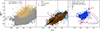 |
Fig. 4. g − r versus r − i colour distribution of simulated magnitude sources from the combined catalogue in the COSMOS2020 field used to optimise the selection function of companions to W0410–0913 in the redshift range 3.531 < z < 3.731. The left panel represents galaxies at lower redshifts (z < 3.531, grey) and higher redshifts (z > 3.731, tan). The middle panel displays stars, X-ray sources, and sources with failed photometric redshift measurements, while the right panel shows galaxies in the targeted redshift range of 3.631 ± 0.1. The solid magenta line represents the optimised selection function at 3.531 < z < 3.731. The grey line shows the colour–redshift track of the LBG composite spectrum of Shapley et al. (2003) with the IGM absorption of Madau (1995) shifted from z = 3.0 to z = 4.25, where the dots indicate Δz = 0.25. We show the representative colours of several classes of galaxies from Coleman et al. (1980) as a function of redshift from z = 0 to z = 3.0. |
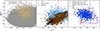 |
Fig. 5. Same as Figure 4 but for optimising the selection of companions to W0831+0140 in the redshift range of 3.812 < z < 4.012. |
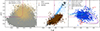 |
Fig. 6. r − i versus i − z colour-distribution-simulated magnitude sources from the combined catalogue in the COSMOS2020 field used to optimise the selection of companions to W2246–0526 in the redshift range 4.601 ± 0.1. Symbols are defined in the same way as described in detail in Figure 4. The figure also shows the selection function adopted by 2023Zewdie based on modified selection criteria of Ouchi et al. (2004, cyan) and the Yoshida et al. (2006, black; See 2023Zewdie for details). The grey line is the colour–redshift track of the LBG composite spectrum of Shapley et al. (2003) with the IGM absorption of Madau (1995) shifted from z = 4.0 to z = 5.5, and the symbols are the same as in Figure 4. |
We estimated the optimal reliability and completeness within the COSMOS fields. We find that the reliability of our optimal selection function for W0410-0913, W0831+0140, and W2246-0526 is 12.9%, 12.3%, and 13.3%, respectively. As can be seen in the left panel of Figures 4, 5, and 6, a higher fraction of the contaminants are galaxies within 0.2 and 0.5 units of redshift. We find that the completeness of our optimal selection function for W0410-0913, W0831+0140, and W2246-0526 is 44.6%, 34.4%, and 61.8%, respectively, although we note that the selection is optimised for contrast and not independently for reliability or completeness.
4. Results and discussion
4.1. Lyman-break galaxy candidates
We applied the optimised selection functions described in the previous section to select LBG candidates in the field around each hot DOG. We eliminated sources brighter than the hot DOGs in the i band and fainter than 3σ in the r and i bands. Sources fainter than the 1σ magnitude limit in the g band are treated as upper limits (1σ) for W0410–0913 and W0831+0140. Similarly, for W2246–0526, we eliminated sources brighter than the hot DOG in the z band, as well as those fainter than 3σ in the i and z bands. Sources fainter than the 1σ magnitude limit in the r band are treated as upper limits (1σ). We found 549, 676, and 96 LBG candidates around W0410–0913, W0831+0140, and W2246–0526, respectively. As mentioned above, the hot DOGs were not positioned at the centre of the IMACS FoV. Within the inner region (see Figure 1 and Section 2), we found 182 and 184 LBG candidates in the field of W0410–0913 and W0831+0140, respectively. These numbers are summarised in Table 3.
Statistical information on the environments around the three hot DOGs studied in this work. We estimate the overdensity using  and
and  , and provide the two area values for W0410–0913 and W0831+0140 for the full and inner region.
Figures 7 and 8 show the colour distributions of detected objects in each field, highlighting the LBG candidates. Figure 8 also shows the selection functions used by 2023Zewdie to identify LBG candidates around W2246–0526, and the modified selection criteria adapted from the studies of Ouchi et al. (2004) and Yoshida et al. (2006). The former identified 37 LBG candidates, while the latter identified 55. The optimised selection function determined in the present work identifies 96 LBG candidates over the same area. However, a direct comparison is difficult as the different selection functions are likely affected by different levels of completeness and reliability. We note, however, that W2246–0526 is not selected as an LBG in our study, nor by either selection function considered by 2023Zewdie. This outcome likely arises from its unique SED, which is influenced by strong dust and an AGN activity. However, the other two hot DOGs are selected as LBG candidates (Figure 7). Unlike W2246–0526, both W0410–0913 and W0831+0140 are selected by our criteria as LBGs, although we note the former is close to the edge of our optimised selection region (see Figure 7).
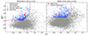 |
Fig. 7. Distribution of the g − r versus r − i colours of sources around W0410–0913 at z = 3.631 (left panel) and W0831+0140 at z = 3.912 (right panel). The hot DOGs are denoted by red filled-circles. In both panels, grey dots represent detected sources, and the blue dots represent the LBG candidates. The magenta lines show the optimised selection criteria based on the simulated magnitude sources from combined COSMOS2020 (see Section 3). In the left panel, the orange filled stars are the LAEs detected by VLT/MUSE observations (Ginolfi et al. 2022). |
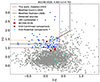 |
Fig. 8. Distribution of the r − i versus i − z colours of sources around W2246–0526 at z = 4.601. The red filled circle, grey and blue dots, and the magenta line have the same meaning as in Fig. 7. Brown filled squares and cyan filled stars are the confirmed and potential companions detected with ALMA observations (Díaz-Santos et al. 2018). The description of the selection function is the same as in Figure 6. |
4.2. Overdensity of LBGs around the hot DOGs
As is evident from Table 3, we find a significantly larger number of LBG candidates around hot DOGs than in the COSMOS2020 field. Assuming the COSMOS2020 field is representative of the average field densities (see below for details), we quantify the overdensities by first comparing the full number of candidates found around each hot DOG (NF) to the number expected in the same area based on COSMOS2020 (NE), namely

where NE is defined as NCOSMOSΨ, with NCOSMOS being the total number of objects selected in COSMOS by the optimised criteria, and  the ratio between the area searched in the COSMOS2020 catalogue (ACOSMOS) and the area searched around the given hot DOG (AHotDOG). This estimate of the overdensity is the simplest, but due to the presence of contaminants it is only a lower limit on the true overdensity. Using the SED classifications and the redshift estimates from the LePhare models presented in COSMOS2020, we can also try to account for contaminants by estimating the overdensity as
where  is defined as
  , with
  being the expected number of galaxies within 0.1 units of redshift from the respective hot DOG (see Eq. (2)), and
  being defined as
  , which is the number of contaminants selected by the optimised criteria in COSMOS2020 (which corresponds to all other categories in Eq. (2)). While in principle this should provide a better characterisation of the overdensities, it is affected by a number of additional sources of systematic uncertainty (primarily the accuracy of photometric redshift in COSMOS2020) as well as being subject to somewhat arbitrary definitions (e.g. the targeted redshift range). To provide a more complete picture, we present both estimates for all hot DOG fields. The true overdensity is expected to be between δ and δ′, with a higher likelihood of being closer to δ′.
We estimate the uncertainty of the overdensity as
while for the contamination-corrected estimate, we calculate the uncertainty as
We report uncertainties based on Poisson statistics, without added systematic uncertainties to account for cosmic variance.
For W0410–0913, considering the entire field of our observations, we find an overdensity of δ = 1.83 ± 0.08 and δ′ = 7.49 ± 0.68, while for W0831+0140, we find δ = 4.67 ± 0.21 and δ′ = 29.17 ± 2.21. The overdensity factors within the inner regions (see Section 2.1 and Figure 1) are δ = 2.36 ± 0.19 and δ′ = 12.38 ± 1.65 for W0410–0913, and δ = 4.38 ± 0.33 and δ′ = 29.50 ± 3.84 for W0831+0140. For W2246–0526 within the much smaller area probed by the GMOS-S imaging, we find δ = 2.36 ± 0.25 and δ′ = 11.60 ± 1.96. We note that Assef et al. (2016) showed that W0831+0140 can be classified as a blue hot DOG; these are objects whose UV/optical SED is dominated by scattered light from the highly obscured central engine (Assef et al. 2016, 2020, 2022). As such, the host may be significantly fainter than the limit adopted above, and could possibly be as faint as the host of W0410-0913. If we only consider LBG candidates fainter than the host galaxy of W0410-0913 (i.e. i > 23.96) in the W0831+0140, we estimate an overdensity of δ = 4.67 ± 0.19 and δ′ = 24.67 ± 1.87. The overdensity factors imply that these hot DOGs live in very dense environments.
Ginolfi et al. (2022) studied an overdensity of LAEs around W0410–0913 using VLT/MUSE, and identified 24 LAEs associated with this hot DOG. In our observations, we detect ten of these LAEs, although only seven have the necessary significance in the i band to be retained in our sample. Of these seven, only three were classified as LBG candidates by our optimised selection function. Of the remaining four, two are very close to the edge of the selection region, while the other two are significantly farther away and may potentially be interlopers.
Figures 9–11 show the surface density of LBG candidates as a function of the continuum band magnitude (i.e. i band for W0410–0913 and W0831+0140, and z band for W2246–0526). The figures also show the distribution of LBG candidates in COSMOS2020 for comparison. A noticeable trend is observed, where the overdensity level seems to diminish towards fainter magnitudes. The diminishing overdensity trend towards fainter magnitudes could be due to several factors, particularly the challenges of detecting faint galaxies and the biases inherent in the selection process. Our observations are not as deep as those from COSMOS, and so we are missing faint objects. When we subtract the contamination in both our field and COSMOS, the difference in overdensity becomes apparent in the figures. We optimise the selection using very small redshift bins, which might also contribute to missing faint sources. However, increasing the redshift bins can lead to more contamination.
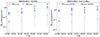 |
Fig. 9. Surface density of LBG candidates around W0410–0913 in the full field (left panel) and in the inner region within the 4.8′ the hot DOGs (right panel). Solid and open symbols show the densities without and with correcting for contaminants, respectively. |
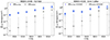 |
Fig. 10. Surface density of LBG candidates around W0831+0140 in the full field (left panel) and in the inner region within the 4.8′ the hot DOG (right panel). Symbols are as in Figure 9. |
2023Zewdie studied the overdensity of LBGs around W2246–0526 using the Subaru Deep Field (SDF) and Subaru/XMM-Newton Deep Field (SXDF) as blank fields, with slightly modified versions of the selection functions presented by Ouchi et al. (2004) and Yoshida et al. (2006). These selection functions have negligible levels of contamination (see discussions in the respective articles as well as in 2023Zewdie). 2023Zewdie found overdensities of δ = 7.1 ± 1.1 (δ = 5.1 ± 1.2) using the modified selection criteria from Ouchi et al. (2004) and the SDF (SXDF) to determine the expected field densities, and an overdensity of δ = 5.2 ± 1.4 using the modified selection criteria from Yoshida et al. (2006) with the SDF for comparison, resulting in an average overdensity of  . The overdensities found by 2023Zewdie are somewhat lower than what we find in the present work, namely δ′ = 11.60 ± 1.96. When applying the modified selection of Ouchi et al. (2004) used by 2023Zewdie to the combined region of the COSMOS2020 field, and taking into account the magnitude range they used, we find that the COSMOS2020 field has a 2.7 (2.5) times higher density of LBG candidates than SDF (SXDF). Similarly, using the modified criteria of Yoshida et al. (2006), we find COSMOS2020 to have a 1.5 times higher density of LBG candidates than SDF. While some of the differences may come from the different filters used (see 2023Zewdie for details), this suggests SDF (which covers a four times smaller area than COSMOS) might be somewhat underdense at the redshift of W2246–0526 (z = 4.601). We note that all fields involved in this work are far from the Galactic plane (GP) and Galactic centre (GC), minimising issues related to stellar contamination. Specifically, the fields for W0410–0913, W0831+0140, and W2246–0526 are 53.14, 23.01, and 39.9 deg away from the GP and 74.36, 131.96, and 135.44 deg away from the GC, respectively. For completeness, we note that COSMOS, SDF, and SXDF are 42.12, 82.62, and 51.49 deg away from the GP and 113.95, 84.16, and 125.56 deg away from the GC, respectively.
4.3. Spatial distribution and angular correlation function
Figures 12, 13, and 14 show the density of LBG candidates as a function of distance from W0410–0913, W0831+0140, and W2246–0526, respectively, measured in 20″ wide annuli centred on the hot DOG (not counting the hot DOG even when selected as an LBG). The overdensity of LBGs shows a profile concentrated around the hot DOGs, suggesting they correspond to the most massive galaxies in these structures and may become the BCGs of the forming clusters once virialised, as suggested by Díaz-Santos et al. (2018). We note that 2023Zewdie failed to identify a density profile clustering around the hot DOG (see Figure 14). The difference is likely due to the fact that our optimised selection function has a higher level of completeness and is able to identify many LBGs missed by 2023Zewdie (see the discussion of overdensities around hot DOGs in their Section 4.1 as well).
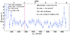 |
Fig. 12. Spatial distribution of LBG candidates as a function of distance from W0410–0913. We count the number of LBG candidates in annuli with 20″ radial intervals, avoiding the inner region of 1″ (7.2 kpc) radius. The vertical dashed red line represents the circle of 280″ in radius shown in Figure 1. |
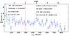 |
Fig. 13. Spatial distribution of LBG candidates as a function of distance from W0831+0140. We count the number of LBG candidates in annuli with 20″ radial intervals, avoiding the inner region of 1″(7.014 kpc) radius. The vertical dashed red lines represent the circle of 295″ radius shown in Figure 1. |
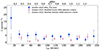 |
Fig. 14. Spatial distribution of LBG candidates as a function of their distance from W2246–0526. We count the number of LBG candidates in annuli with 20″ radial intervals, excluding the inner region of 2″(13.072 kpc) radius. We adapted this analysis from 2023Zewdie. The magenta open circles and grey open squares represent the selected LBG candidates based on modified selection criteria from 2023Zewdie. These selections have been corrected for detection completeness. For clarity, we shifted the surface density of LBG candidates selected by the modified Ouchi et al. (2004) selection criteria by +5″ on the x-axis. |
Further characterisation of the spatial distribution can be achieved by looking at their clustering. We use the two-point angular correlation, ω(θ), in each field to provide further evidence that these candidates are truly associated with one another. Specifically, ω(θ) is defined as the excess probability δP of finding objects with an angular separation of θ from each other, such that
![$$ \begin{aligned} \delta P=n^2[1+\omega (\theta )]\delta \Omega _1 \delta \Omega _2 ,\end{aligned} $$](/articles/aa/full_html/2025/02/aa51403-24/aa51403-24-eq22.gif)
where n is the mean number density, and δΩ1 and δΩ2 are the elements of the solid angle with a separation angle θ.
We used the estimator proposed by Landy & Szalay (1993) to calculate the two-point angular correlation function, namely
where DD(θ) is the number of pairs of selected LBGs with angular separations of between θ and θ + Δθ, RR(θ) is the number of pairs from random catalogues with the same geometry as the selected LBGs, and DR(θ) is the number of cross-pairs between data and random galaxies. Here, nD and nR are the total number densities of galaxies in the data and random catalogues, while NDD = nD * (nD − 1)/2, NRR = nR * (nR − 1)/2, and NDR = nD * nR are the total numbers of data-data pairs, random-random pairs, and data-random pairs, respectively. This galaxy correlation function estimator is widely used in the literature (e.g. Croom et al. 2005; Lee et al. 2006; Overzier et al. 2006a). We estimate the errors assuming Poisson statistics (Croom et al. 2005):
To compute the DR and RR terms, we used 10 000 random sources uniformly distributed within an area equivalent to that of each field. We then applied the same masks described in Section 2 for each field and computed the correlation functions. The results are shown in Figures 15.
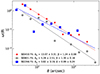 |
Fig. 15. Angular auto-correlation function of the selected LBG candidates around W0410–0913 (red stars), W0831+0140 (grey solid circles), and W2246–0526 (blue squares). We used logarithmic binning of the separations to ensure sufficient pair counts at small separations. The lines represent the power-law fits (red dotted lines): for W0410–0913 and W0831+0140, the separation angle ranges from 3 arcseconds to 480 arcseconds, with power-law fits (grey solid lines) of Aω = 13.07 ± 3.31 and β = 1.244 ± 0.08; and Aω = 5.28 ± 2.51 and β = 1.30 ± 0.16, respectively. For W2246–0526, the separation angle ranges from 2 arcseconds to 480 arcseconds, with power-law fits (blue dashed lines) of Aω = 3.82 ± 3.19 and β = 0.99 ± 0.24. |
The angular auto-correlation function is often expressed in the form of a power law (e.g. Roche & Eales 1999):
where Aω is the amplitude of the auto-correlation function and β is the slope or power-law index. As shown in Figures 15, which show the fit of the angular auto-correlation functions, for W0410-0913, Aω = 13.07 ± 3.31, and β = 1.244 ± 0.08; for W0831+0140, Aω = 5.28 ± 2.51, and β = 1.30 ± 0.16 and for W2246–0526, Aω = 3.82 ± 3.19, and β = 0.99 ± 0.24. We find ahigher amplitude and slope, indicating strong clustering at smaller scales.
Several analyses have fitted the power law by fixing β = 0.8 and β = 0.6. We also fixed the power-law index, β, value to estimate the clustering amplitude in each field, as shown in Table 4. Ouchi et al. (2001) studied the clustering amplitude for three fields at z ∼ 4, and Harikane et al. (2016) studied three fields at 3.8 < z < 6.8 by fixing β = 0.8 and found that Aω ranged from 0.56 ± 0.25 to 0.97 ± 0.57 and from 0.2 ± 0.10 to 8.8 ± 3.4, respectively. Similarly, Lee et al. (2006) studied ten fields at 3.5 < z < 5.5 by fixing β = 0.6 and found that Aω ranged from  to
to  . These three studies measured clustering amplitudes in field studies. We find that the clustering amplitude in our hot DOGs is somewhat higher than that observed in similar redshift studies conducted in the field. Specifically, at β = 0.8, we find a higher clustering signal than in the SDF field studies (Ouchi et al. 2001), and a weaker clustering at β = 0.6, although this latter is similar to the clustering signal found in the two Great Observatories Deep Origins Survey (GOODS) field studies (Lee et al. 2006). The rapid decrease in the clustering signal with decreasing β values suggests that galaxies are more clustered at smaller angular separations.
Summary of the clustering amplitude with the power-law model using best-fitting parameters (Aω and β) and two fixed power-law indices of the correlation function.
4.4. Overdensities around quasars and radio galaxies
2023Zewdie conducted a comparison of the overdensities observed around hot DOGs, quasars, and radio galaxies at different redshifts collected from the literature (see their Figure 12 and the discussion and references in their Section 4). The comparison encompasses various tracers, such as LBGs around quasars (Overzier et al. 2006b; Utsumi et al. 2010; Morselli et al. 2014; Balmaverde et al. 2017; García-Vergara et al. 2017; Ota et al. 2018; Mignoli et al. 2020), and radio galaxies (Miley et al. 2004; Intema et al. 2006; Overzier et al. 2008); and LAEs around quasars (García-Vergara et al. 2019), radio galaxies (Venemans et al. 2002, 2004), and hot DOGs (Ginolfi et al. 2022). Additionally, the comparison includes red, distant galaxies around a hot DOG (Luo et al. 2022) and 24 μm sources around radio galaxies (Mayo et al. 2012).
Ouchi et al. (2004) studied the properties of photometrically selected LBGs using deep SDF and SXDF imaging in R, i, z bands, finding that the selected LBGs had reasonably high completeness and low contamination from interlopers. 2023Zewdie modified the Ouchi et al. (2004) selection criteria by taking into account the filter curve and the IGM absorption model of Madau (1995), aiming to account for differences in the filters to ensure that the same sources were targeted as those targeted by Ouchi et al., which is necessary in order to estimate the overdensity. 2023Zewdie also checked the modified selection criteria by overplotting different types of stars (including main sequence, giant, and supergiant stellar atmosphere models from Castelli & Kurucz 2004, and M and L dwarfs from Burgasser 2014) and low-redshift galaxy templates from Coleman et al. (1980), shifted to redshifts from z = 0 to 3 (see Figures 4–6). 2023Zewdie found no contamination from these interlopers, as shown in their Figure 4.
Here, we have updated their comparison by adding the overdensity factors around the three hot DOGs studied in this work (see Figure 16), providing further evidence that hot DOGs may live in some of the densest structures at their redshifts. For completeness, we show the overdensity for the hot DOG environments both with (δ) and without (δ′) correcting for contaminants (see section 4.2 for details). The denseness of these environments may be related to their unique properties, such as their extreme infrared luminosities and high SMBH accretion rates. Given the small sample size, we are not able to draw strong conclusions as to the overdensity factor variation as a function of redshift.
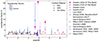 |
Fig. 16. Overdensity around high-redshift radio galaxies, quasars, and hot DOGs as a function of redshift adapted from 2023Zewdie. We added the three hot DOGs overdensities (δ′ filled star and δ open star) that were found using the optimised selection criteria. The red horizontal line indicates a null overdensity. (*We note that, in the literature, overdensity is defined as |
5. Conclusions
In this study, we investigated the environments of three hot DOGs by looking for companion LBGs using IMACS and GMOS-S photometry. In order to improve our sensitivity to LBGs, we developed a novel process to optimise the photometric selection criteria using the COSMOS2020 combined catalogue. Specifically, we used the HSC photometry of this field combined with its accurate photometric redshifts and SED classifications to adjust the colour selection criteria in order to target the galaxies at the specific redshift of each hot DOG we study. We summarise our results below.
-
For the hot DOG W0410-0916 at z = 3.631, we find an overdensity of δ = 1.83 ± 0.08 when considering the whole FoV of the IMACS imaging (14.6×14.6 Mpc2) compared to the density of targets selected using the same criteria in the COSMOS2020 catalogue. When focusing on the region within 2 Mpc of the hot DOG, we find instead δ = 2.36 ± 0.19. When accounting for potential contaminants based on the redshifts and classifications of COSMOS2020, these overdensities increase to δ′ = 7.49 ± 0.68 and 12.38 ± 1.65, respectively. Our results are consistent with the overdensity of LAEs of 14
 found by Ginolfi et al. (2022) within a 0.4 Mpc radius of the hot DOG.
 -
For W0831+0140 at z = 3.912, we also find an overdense field compared to COSMOS2020 with δ = 4.67 ± 0.21 within the entire IMACS FOV and δ = 4.38 ± 0.33 when focusing on the region within 2 Mpc of the hot DOG. When attempting to remove contaminants, these estimates increase to δ′ = 30.9 ± 2.0 and 29.4 ± 3.84, respectively.
-
We reanalysed the GMOS-S observations presented by 2023Zewdie for W2246–0526 at z = 4.601 to identify LBG companions using our method to optimise the selection criteria. We find an overdensity within the area of 4.7 × 4.7 arcmin2 of δ = 2.5 ± 0.5 that increases to δ′ = 11.60 ± 1.96 when attempting to remove contaminants. 2023Zewdie instead found an overdensity of
 when using the selection criteria from Ouchi et al. (2004) and Yoshida et al. (2006) and comparing to the target density found in the SDF and SXDF. We find that, while some of the difference could be explained by the different levels of contamination of the selection criteria and the different filters used, much of the difference may come from SDF/SXDF being underdense by a factor of about 2 when compared to COSMOS2020.
 -
Analysing the radial distribution of LBG candidates with respect to the hot DOGs, we find that in all three fields the overdensities are concentrated around the hot DOGs (Figures 12, 13, and 14).
We also compared our work with previous overdensity studies involving tracers such as LBGs, LAEs, and other companions around hot DOGs, quasars, and radio galaxies. We find hot DOGs may have some of the densest environments among luminous, active galaxies. Our results therefore suggest that hot DOGs are good tracers of dense protoclusters. Additional spectroscopic follow-up observations are necessary to further constrain the properties of the environments of these objects and to confirm whether or not hot DOGs represent an early stage of formation for the BCGs found in the local Universe.
The COSMOS2020 catalogueis available for download at https://cosmos2020.calet.org/
Acknowledgments
We thank the anonymous referee for their constructive comments and suggestions, which improved this article. DZ acknowledges the support of ANID fellowship grants, grant No. 21211531. RJA was supported by FONDECYT grants number 191124 and 1231718, and by the ANID BASAL project FB210003. SIL is supported in part by the National Research Foundation (NRF) of South Africa (NRF Grant Number: 146053). Any opinion, finding, and conclusion or recommendation expressed in this material is that of the author(s), and the NRF does not accept any liability in this regard. JGL acknowledges support from “Programa de Inserción Académica 2024 Vicerrectoría Académica y Prorrectoría Pontificia Universidad Católica de Chile”. The work of PRME and DS was carried out at the Jet Propulsion Laboratory, California Institute of Technology, under a contract with NASA. TDS acknowledges the research project was supported by the Hellenic Foundation for Research and Innovation (HFRI) under the “2nd Call for HFRI Research Projects to support Faculty Members & Researchers” (Project Number: 03382).
References
- Angulo, R. E., Springel, V., White, S. D. M., et al. 2012, MNRAS, 425, 2722 [NASA ADS] [CrossRef] [Google Scholar]
- Arnouts, S., Moscardini, L., Vanzella, E., et al. 2002, MNRAS, 329, 355 [Google Scholar]
- Assef, R. J., Eisenhardt, P. R. M., Stern, D., et al. 2015, ApJ, 804, 27 [Google Scholar]
- Assef, R. J., Walton, D. J., Brightman, M., et al. 2016, ApJ, 819, 111 [Google Scholar]
- Assef, R. J., Brightman, M., Walton, D. J., et al. 2020, ApJ, 897, 112 [NASA ADS] [CrossRef] [Google Scholar]
- Assef, R. J., Bauer, F. E., Blain, A. W., et al. 2022, ApJ, 934, 101 [NASA ADS] [CrossRef] [Google Scholar]
- Balmaverde, B., Gilli, R., Mignoli, M., et al. 2017, A&A, 606, A23 [NASA ADS] [CrossRef] [EDP Sciences] [Google Scholar]
- Bañados, E., Venemans, B., Walter, F., et al. 2013, ApJ, 773, 178 [CrossRef] [Google Scholar]
- Bañados, E., Venemans, B. P., Mazzucchelli, C., et al. 2018, Nature, 553, 473 [Google Scholar]
- Bertin, E., & Arnouts, S. 1996, A&AS, 117, 393 [NASA ADS] [CrossRef] [EDP Sciences] [Google Scholar]
- Bertin, E., Mellier, Y., Radovich, M., et al. 2002, in Astronomical Data Analysis Software and Systems XI, eds. D. A. Bohlender, D. Durand, & T. H. Handley, Astronomical Society of the Pacific Conference Series, 281, 228 [NASA ADS] [Google Scholar]
- Bosman, S. E. I., Kakiichi, K., Meyer, R. A., et al. 2020, ApJ, 896, 49 [Google Scholar]
- Brammer, G. B., van Dokkum, P. G., & Coppi, P. 2008, ApJ, 686, 1503 [Google Scholar]
- Burgasser, A. J. 2014, Astronomical Society of India Conference Series, 11, 7 [Google Scholar]
- Castelli, F., & Kurucz, R. L. 2004, A&A, 419, 725 [NASA ADS] [CrossRef] [EDP Sciences] [Google Scholar]
- Champagne, J. B., Casey, C. M., Finkelstein, S. L., et al. 2023, ApJ, 952, 99 [NASA ADS] [CrossRef] [Google Scholar]
- Coleman, G. D., Wu, C. C., & Weedman, D. W. 1980, ApJS, 43, 393 [CrossRef] [Google Scholar]
- Croom, S. M., Boyle, B. J., Shanks, T., et al. 2005, MNRAS, 356, 415 [NASA ADS] [CrossRef] [Google Scholar]
- Dayal, P., Rossi, E. M., Shiralilou, B., et al. 2019, MNRAS, 486, 2336 [Google Scholar]
- Díaz-Santos, T., Assef, R. J., Blain, A. W., et al. 2016, ApJ, 816, L6 [Google Scholar]
- Díaz-Santos, T., Assef, R. J., Blain, A. W., et al. 2018, Science, 362, 1034 [Google Scholar]
- Eisenhardt, P. R. M., Wu, J., Tsai, C.-W., et al. 2012, ApJ, 755, 173 [Google Scholar]
- Erben, T., Schirmer, M., Dietrich, J. P., et al. 2005, Astron. Nachr., 326, 432 [NASA ADS] [CrossRef] [Google Scholar]
- Fan, L., Jones, S. F., Han, Y., & Knudsen, K. K. 2017, PASP, 129, 124101 [NASA ADS] [CrossRef] [Google Scholar]
- Fan, X., Bañados, E., & Simcoe, R. A. 2023, ARA&A, 61, 373 [NASA ADS] [CrossRef] [Google Scholar]
- Finnerty, L., Larson, K., Soifer, B. T., et al. 2020, ApJ, 905, 16 [Google Scholar]
- Gaia Collaboration (Vallenari, A., et al.) 2023, A&A, 674, A1 [NASA ADS] [CrossRef] [EDP Sciences] [Google Scholar]
- García-Vergara, C., Hennawi, J. F., Barrientos, L. F., & Rix, H.-W. 2017, ApJ, 848, 7 [CrossRef] [Google Scholar]
- García-Vergara, C., Hennawi, J. F., Barrientos, L. F., & Arrigoni Battaia, F. 2019, ApJ, 886, 79 [CrossRef] [Google Scholar]
- Ginolfi, M., Piconcelli, E., Zappacosta, L., et al. 2022, Nat. Commun., 13, 4574 [NASA ADS] [CrossRef] [Google Scholar]
- Harikane, Y., Ouchi, M., Ono, Y., et al. 2016, ApJ, 821, 123 [NASA ADS] [CrossRef] [Google Scholar]
- Hoaglin, D. C., Mosteller, F., & Tukey, J. W. 1983, Understanding Robust and Exploratory Data Anlysis (New York: Wiley) [Google Scholar]
- Husband, K., Bremer, M. N., Stanway, E. R., et al. 2013, MNRAS, 432, 2869 [NASA ADS] [CrossRef] [Google Scholar]
- Ilbert, O., Arnouts, S., McCracken, H. J., et al. 2006, A&A, 457, 841 [NASA ADS] [CrossRef] [EDP Sciences] [Google Scholar]
- Inayoshi, K., Visbal, E., & Haiman, Z. 2020, ARA&A, 58, 27 [NASA ADS] [CrossRef] [Google Scholar]
- Intema, H. T., Venemans, B. P., Kurk, J. D., et al. 2006, A&A, 456, 433 [NASA ADS] [CrossRef] [EDP Sciences] [Google Scholar]
- Jones, S. F., Blain, A. W., Stern, D., et al. 2014, MNRAS, 443, 146 [Google Scholar]
- Jones, S. F., Blain, A. W., Assef, R. J., et al. 2017, MNRAS, 469, 4565 [Google Scholar]
- Jun, H. D., Assef, R. J., Bauer, F. E., et al. 2020, ApJ, 888, 110 [Google Scholar]
- Kashikawa, N., Kitayama, T., Doi, M., et al. 2007, ApJ, 663, 765 [NASA ADS] [CrossRef] [Google Scholar]
- Kim, S., Stiavelli, M., Trenti, M., et al. 2009, ApJ, 695, 809 [NASA ADS] [CrossRef] [Google Scholar]
- Lambert, T. S., Assef, R. J., Mazzucchelli, C., et al. 2024, A&A, 689, A331 [NASA ADS] [CrossRef] [EDP Sciences] [Google Scholar]
- Landy, S. D., & Szalay, A. S. 1993, ApJ, 412, 64 [Google Scholar]
- Lee, K.-S., Giavalisco, M., Gnedin, O. Y., et al. 2006, ApJ, 642, 63 [NASA ADS] [CrossRef] [Google Scholar]
- Li, Y., Hernquist, L., Robertson, B., et al. 2007, ApJ, 665, 187 [Google Scholar]
- Li, G., Assef, R. J., Tsai, C.-W., et al. 2024, ApJ, 971, 40 [NASA ADS] [CrossRef] [Google Scholar]
- Luo, Y., Fan, L., Zou, H., et al. 2022, ApJ, 935, 80 [NASA ADS] [CrossRef] [Google Scholar]
- Madau, P. 1995, ApJ, 441, 18 [NASA ADS] [CrossRef] [Google Scholar]
- Mayo, J. H., Vernet, J., De Breuck, C., et al. 2012, A&A, 539, A33 [NASA ADS] [CrossRef] [EDP Sciences] [Google Scholar]
- Mazzucchelli, C., Bañados, E., Decarli, R., et al. 2017, ApJ, 834, 83 [NASA ADS] [CrossRef] [Google Scholar]
- Mignoli, M., Gilli, R., Decarli, R., et al. 2020, A&A, 642, L1 [EDP Sciences] [Google Scholar]
- Miley, G. K., Overzier, R. A., Tsvetanov, Z. I., et al. 2004, Nature, 427, 47 [NASA ADS] [CrossRef] [Google Scholar]
- Morselli, L., Mignoli, M., Gilli, R., et al. 2014, A&A, 568, A1 [NASA ADS] [CrossRef] [EDP Sciences] [Google Scholar]
- Noirot, G., Stern, D., Mei, S., et al. 2018, ApJ, 859, 38 [NASA ADS] [CrossRef] [Google Scholar]
- Ota, K., Venemans, B. P., Taniguchi, Y., et al. 2018, ApJ, 856, 109 [NASA ADS] [CrossRef] [Google Scholar]
- Ouchi, M., Shimasaku, K., Okamura, S., et al. 2001, ApJ, 558, L83 [NASA ADS] [CrossRef] [Google Scholar]
- Ouchi, M., Shimasaku, K., Okamura, S., et al. 2004, ApJ, 611, 660 [Google Scholar]
- Overzier, R. A., Bouwens, R. J., Illingworth, G. D., & Franx, M. 2006a, ApJ, 648, L5 [NASA ADS] [CrossRef] [Google Scholar]
- Overzier, R. A., Miley, G. K., Bouwens, R. J., et al. 2006b, ApJ, 637, 58 [NASA ADS] [CrossRef] [Google Scholar]
- Overzier, R. A., Bouwens, R. J., Cross, N. J. G., et al. 2008, ApJ, 673, 143 [NASA ADS] [CrossRef] [Google Scholar]
- Overzier, R. A., Guo, Q., Kauffmann, G., et al. 2009, MNRAS, 394, 577 [NASA ADS] [CrossRef] [Google Scholar]
- Roche, N., & Eales, S. A. 1999, MNRAS, 307, 703 [NASA ADS] [CrossRef] [Google Scholar]
- Schirmer, M. 2013, ApJS, 209, 21 [NASA ADS] [CrossRef] [Google Scholar]
- Scoville, N., Aussel, H., Brusa, M., et al. 2007, ApJS, 172, 1 [Google Scholar]
- Shapley, A. E., Steidel, C. C., Pettini, M., & Adelberger, K. L. 2003, ApJ, 588, 65 [Google Scholar]
- Soltan, A. 1982, MNRAS, 200, 115 [Google Scholar]
- Steidel, C. C., Adelberger, K. L., Shapley, A. E., et al. 2003, ApJ, 592, 728 [Google Scholar]
- Stern, D., Lansbury, G. B., Assef, R. J., et al. 2014, ApJ, 794, 102 [Google Scholar]
- Tachibana, Y., & Miller, A. A. 2018, PASP, 130, 128001 [NASA ADS] [CrossRef] [Google Scholar]
- Tonry, J. L., Stubbs, C. W., Lykke, K. R., et al. 2012, ApJ, 750, 99 [Google Scholar]
- Tsai, C.-W., Eisenhardt, P. R. M., Wu, J., et al. 2015, ApJ, 805, 90 [Google Scholar]
- Tsai, C.-W., Eisenhardt, P. R. M., Jun, H. D., et al. 2018, ApJ, 868, 15 [NASA ADS] [CrossRef] [Google Scholar]
- Uchiyama, H., Toshikawa, J., Kashikawa, N., et al. 2018, PASJ, 70, S32 [NASA ADS] [CrossRef] [Google Scholar]
- Utsumi, Y., Goto, T., Kashikawa, N., et al. 2010, ApJ, 721, 1680 [NASA ADS] [CrossRef] [Google Scholar]
- Venemans, B. P., Kurk, J. D., Miley, G. K., et al. 2002, ApJ, 569, L11 [NASA ADS] [CrossRef] [Google Scholar]
- Venemans, B. P., Röttgering, H. J. A., Overzier, R. A., et al. 2004, A&A, 424, L17 [NASA ADS] [CrossRef] [EDP Sciences] [Google Scholar]
- Venemans, B. P., Röttgering, H. J. A., Miley, G. K., et al. 2007, A&A, 461, 823 [NASA ADS] [CrossRef] [EDP Sciences] [Google Scholar]
- Wang, F., Yang, J., Fan, X., et al. 2021, ApJ, 907, L1 [Google Scholar]
- Weaver, J. R., Kauffmann, O. B., Ilbert, O., et al. 2022, ApJS, 258, 11 [NASA ADS] [CrossRef] [Google Scholar]
- Wright, E. L., Eisenhardt, P. R. M., Mainzer, A. K., et al. 2010, AJ, 140, 1868 [Google Scholar]
- Wu, J., Tsai, C.-W., Sayers, J., et al. 2012, ApJ, 756, 96 [Google Scholar]
- Wylezalek, D., Galametz, A., Stern, D., et al. 2013, ApJ, 769, 79 [NASA ADS] [CrossRef] [Google Scholar]
- Yoshida, M., Shimasaku, K., Kashikawa, N., et al. 2006, ApJ, 653, 988 [NASA ADS] [CrossRef] [Google Scholar]
- Zewdie, D., Assef, R. J., Mazzucchelli, C., et al. 2023, A&A, 677, A54 [NASA ADS] [CrossRef] [EDP Sciences] [Google Scholar]
- Zheng, W., Overzier, R. A., Bouwens, R. J., et al. 2006, ApJ, 640, 574 [NASA ADS] [CrossRef] [Google Scholar]
All Tables
Summary of IMACS and GMOS-S observations used in this work. All data were acquired during the night of 25 November 2019 for both IMACS observations and nights of 16/23/27 September 2017 for W2246–0526 GMOS-S observations (2023Zewdie).
Constants to model the photometric uncertainty as a function of magnitude in our fields.
Statistical information on the environments around the three hot DOGs studied in this work. We estimate the overdensity using and , and provide the two area values for W0410–0913 and W0831+0140 for the full and inner region.
Summary of the clustering amplitude with the power-law model using best-fitting parameters (Aω and β) and two fixed power-law indices of the correlation function.
All Figures
|
Fig. 1. r-band image of W0410–0913 (left-panel) and W0831+0140 (right-panel). In both panels, black circles and polygons show the masked area that we did not use for our LBG selection (see Section 2.1 for details). The blue circles and arrows indicate the hot DOGs positions, and the cyan circle represents the largest area centred on the hot DOG within the image bounds. The red circles are candidate LBG companions. |
| In the text | |
|
Fig. 2. i-band image of W2246–0526. The solid orange circle indicates the position of this hot DOG. The blue circles show the LBG candidates selected by 2023Zewdie using the modified selection criteria and with optimised selection criteria. The black circles and rectangles show the masked area. The red circles and rectangles show the LBG candidates only selected by 2023Zewdie and using optimised selection criteria, respectively. Figure adapted from 2023Zewdie. |
| In the text | |
|
Fig. 3. Composite LBG spectrum from Shapley et al. (2003) shifted to z = 3.631 (black dashed lines) and z = 3.912 (grey solid lines), used for optimising the selection function for the W0410–0913 and W0831+0140 fields, respectively. After accounting for quantum efficiency and atmospheric transmission, the red and blue lines represent the HSC filter curves (used for optimisation and the blank field) and the IMACS filter curves (used for W0410–0913 and W0831+0140), respectively. |
| In the text | |
|
Fig. 4. g − r versus r − i colour distribution of simulated magnitude sources from the combined catalogue in the COSMOS2020 field used to optimise the selection function of companions to W0410–0913 in the redshift range 3.531 < z < 3.731. The left panel represents galaxies at lower redshifts (z < 3.531, grey) and higher redshifts (z > 3.731, tan). The middle panel displays stars, X-ray sources, and sources with failed photometric redshift measurements, while the right panel shows galaxies in the targeted redshift range of 3.631 ± 0.1. The solid magenta line represents the optimised selection function at 3.531 < z < 3.731. The grey line shows the colour–redshift track of the LBG composite spectrum of Shapley et al. (2003) with the IGM absorption of Madau (1995) shifted from z = 3.0 to z = 4.25, where the dots indicate Δz = 0.25. We show the representative colours of several classes of galaxies from Coleman et al. (1980) as a function of redshift from z = 0 to z = 3.0. |
| In the text | |
|
Fig. 5. Same as Figure 4 but for optimising the selection of companions to W0831+0140 in the redshift range of 3.812 < z < 4.012. |
| In the text | |
|
Fig. 6. r − i versus i − z colour-distribution-simulated magnitude sources from the combined catalogue in the COSMOS2020 field used to optimise the selection of companions to W2246–0526 in the redshift range 4.601 ± 0.1. Symbols are defined in the same way as described in detail in Figure 4. The figure also shows the selection function adopted by 2023Zewdie based on modified selection criteria of Ouchi et al. (2004, cyan) and the Yoshida et al. (2006, black; See 2023Zewdie for details). The grey line is the colour–redshift track of the LBG composite spectrum of Shapley et al. (2003) with the IGM absorption of Madau (1995) shifted from z = 4.0 to z = 5.5, and the symbols are the same as in Figure 4. |
| In the text | |
|
Fig. 7. Distribution of the g − r versus r − i colours of sources around W0410–0913 at z = 3.631 (left panel) and W0831+0140 at z = 3.912 (right panel). The hot DOGs are denoted by red filled-circles. In both panels, grey dots represent detected sources, and the blue dots represent the LBG candidates. The magenta lines show the optimised selection criteria based on the simulated magnitude sources from combined COSMOS2020 (see Section 3). In the left panel, the orange filled stars are the LAEs detected by VLT/MUSE observations (Ginolfi et al. 2022). |
| In the text | |
|
Fig. 8. Distribution of the r − i versus i − z colours of sources around W2246–0526 at z = 4.601. The red filled circle, grey and blue dots, and the magenta line have the same meaning as in Fig. 7. Brown filled squares and cyan filled stars are the confirmed and potential companions detected with ALMA observations (Díaz-Santos et al. 2018). The description of the selection function is the same as in Figure 6. |
| In the text | |
|
Fig. 9. Surface density of LBG candidates around W0410–0913 in the full field (left panel) and in the inner region within the 4.8′ the hot DOGs (right panel). Solid and open symbols show the densities without and with correcting for contaminants, respectively. |
| In the text | |
|
Fig. 10. Surface density of LBG candidates around W0831+0140 in the full field (left panel) and in the inner region within the 4.8′ the hot DOG (right panel). Symbols are as in Figure 9. |
| In the text | |
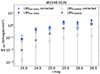 |
Fig. 11. Surface density of the LBG candidates around W2246–0526. For plot details, see Figure 9. |
| In the text | |
|
Fig. 12. Spatial distribution of LBG candidates as a function of distance from W0410–0913. We count the number of LBG candidates in annuli with 20″ radial intervals, avoiding the inner region of 1″ (7.2 kpc) radius. The vertical dashed red line represents the circle of 280″ in radius shown in Figure 1. |
| In the text | |
|
Fig. 13. Spatial distribution of LBG candidates as a function of distance from W0831+0140. We count the number of LBG candidates in annuli with 20″ radial intervals, avoiding the inner region of 1″(7.014 kpc) radius. The vertical dashed red lines represent the circle of 295″ radius shown in Figure 1. |
| In the text | |
|
Fig. 14. Spatial distribution of LBG candidates as a function of their distance from W2246–0526. We count the number of LBG candidates in annuli with 20″ radial intervals, excluding the inner region of 2″(13.072 kpc) radius. We adapted this analysis from 2023Zewdie. The magenta open circles and grey open squares represent the selected LBG candidates based on modified selection criteria from 2023Zewdie. These selections have been corrected for detection completeness. For clarity, we shifted the surface density of LBG candidates selected by the modified Ouchi et al. (2004) selection criteria by +5″ on the x-axis. |
| In the text | |
|
Fig. 15. Angular auto-correlation function of the selected LBG candidates around W0410–0913 (red stars), W0831+0140 (grey solid circles), and W2246–0526 (blue squares). We used logarithmic binning of the separations to ensure sufficient pair counts at small separations. The lines represent the power-law fits (red dotted lines): for W0410–0913 and W0831+0140, the separation angle ranges from 3 arcseconds to 480 arcseconds, with power-law fits (grey solid lines) of Aω = 13.07 ± 3.31 and β = 1.244 ± 0.08; and Aω = 5.28 ± 2.51 and β = 1.30 ± 0.16, respectively. For W2246–0526, the separation angle ranges from 2 arcseconds to 480 arcseconds, with power-law fits (blue dashed lines) of Aω = 3.82 ± 3.19 and β = 0.99 ± 0.24. |
| In the text | |
|
Fig. 16. Overdensity around high-redshift radio galaxies, quasars, and hot DOGs as a function of redshift adapted from 2023Zewdie. We added the three hot DOGs overdensities (δ′ filled star and δ open star) that were found using the optimised selection criteria. The red horizontal line indicates a null overdensity. (*We note that, in the literature, overdensity is defined as |
| In the text | |
Current usage metrics show cumulative count of Article Views (full-text article views including HTML views, PDF and ePub downloads, according to the available data) and Abstracts Views on Vision4Press platform.
Data correspond to usage on the plateform after 2015. The current usage metrics is available 48-96 hours after online publication and is updated daily on week days.
Initial download of the metrics may take a while.