| Issue |
A&A
Volume 689, September 2024
|
|
|---|---|---|
| Article Number | A327 | |
| Number of page(s) | 13 | |
| Section | Extragalactic astronomy | |
| DOI | https://doi.org/10.1051/0004-6361/202449732 | |
| Published online | 24 September 2024 | |
The fundamental plane of black hole activity for low-luminosity radio active galactic nuclei across 0 < z < 4
1
School of Astronomy and Space Science, Nanjing University, 163 Xianlin Avenue, Nanjing 210023, People’s Republic of China
2
Key Laboratory of Modern Astronomy and Astrophysics, Nanjing University, Ministry of Education, 163 Xianlin Avenue, Nanjing 210023, People’s Republic of China
3
Kavli Institute for Astronomy and Astrophysics, Peking University, Beijing 100871, People’s Republic of China
4
Department of Astronomy, School of Physics, Peking University, Beijing 100871, People’s Republic of China
5
Department of Pure and Applied Physics, Waseda University, 3-4-1 Okubo, Shinjuku, Tokyo 169-8555, Japan
Received:
26
February
2024
Accepted:
10
June
2024
Abstract
Context. The fundamental plane of black hole activity describes the correlation between radio luminosity (LR), X-ray luminosity (LX), and black hole mass (MBH). It reflects a connection between the accretion disc and the jet. However, the dependence of the fundamental plane on various physical properties of active galactic nuclei (AGNs) and host galaxies remains unclear, especially for low-luminosity AGNs, which is important for understanding the accretion physics in AGNs.
Aims. Here, we explore the dependence of the fundamental plane on the radio loudness, Eddington-ratio (λEdd), redshift, and galaxy star formation properties (star-forming galaxies and quiescent galaxies) across 0.1 < z ≤ 4 for radio AGNs. Based on current deep and large surveys, our studies can extend to lower luminosities and higher redshifts.
Methods. From the deep and large multi-wavelength surveys in the GOODS-N, GOODS-S, and COSMOS/UltraVISTA fields, we constructed a large and homogeneous radio AGN sample consisting of 208 objects with available estimates for LR and LX. Then we divided the radio AGN sample into 141 radio-quiet AGNs and 67 radio-loud AGNs according to the radio loudness defined by the ratio of LR to LX, and explored the dependence of the fundamental plane on different physical properties of the two populations, separately.
Results. The ratio of LR to LX shows a bimodal distribution that is well described by two single Gaussian models. The cross point between these two Gaussian components corresponds to a radio-loudness threshold of log(LR/LX) = − 2.73. The radio-quiet AGNs have a significantly larger Eddington ratio than the radio-loud AGNs. Our radio-quiet and radio-loud AGNs show a significantly different fundamental plane, which indicates a significant dependence of the fundamental plane on the radio loudness. For both radio-quiet and radio-loud AGNs, the fundamental plane shows a significant dependence on λEdd, but no dependence on redshift. The fundamental plane shows a significant dependence on the galaxy star formation properties for radio-quiet AGNs, while for radio-loud AGNs this dependence disappears.
Conclusions. The fundamental plane sheds important light on the accretion physics and X-ray emission origins of central engines. X-ray emission of radio-quiet AGNs at 0.01 < λEdd < 0.1 are produced by a combination of advection-dominated accretion flow (ADAF) and synchrotron radiation from the jet, while at 0.1 < λEdd < 1 they mainly follow the synchrotron jet model. The origins of X-ray emission of radio-loud AGNs are consistent with a combination of ADAF and the synchrotron jet model at λEdd < 0.01, agree with the synchrotron jet model at 0.01 < λEdd < 0.1, and follow a combination of the standard thin disc and a jet model at λEdd > 0.1.
Key words: galaxies: active / galaxies: general / galaxies: nuclei
Corresponding authors; This email address is being protected from spambots. You need JavaScript enabled to view it. , This email address is being protected from spambots. You need JavaScript enabled to view it. .
© The Authors 2024
 Open Access article, published by EDP Sciences, under the terms of the Creative Commons Attribution License (https://creativecommons.org/licenses/by/4.0), which permits unrestricted use, distribution, and reproduction in any medium, provided the original work is properly cited.
This article is published in open access under the Subscribe to Open model. This email address is being protected from spambots. You need JavaScript enabled to view it. to support open access publication.
1. Introduction
Accreting supermassive black holes (SMBHs), also known as active galactic nuclei (AGNs), emit immense energy across the whole electromagnetic spectrum, which is believed to have a great impact on the growth and evolution of host galaxies (Fabian 2012; King & Pounds 2015, for reviews). Thus, AGNs are ideal laboratories in which to explore both accretion physics around black holes and their connection with host galaxies. Accretion physics around black holes are found to be scale-invariant across black hole mass scale from ∼10 solar masses of X-ray binaries (XRBs) to 106 ∼ 1010 solar masses of SMBHs (Merloni et al. 2003; Falcke et al. 2004; Done & Gierliński 2005; McHardy et al. 2006; Körding 2014; Ruan et al. 2019). One of the most prominent pieces of evidence supporting the unification of XRBs and SMBHs is the fundamental plane of black hole activity (Merloni et al. 2003; Falcke et al. 2004 and references therein) that is characterized by a nonlinear empirical relation given by radio luminosity, X-ray luminosity, and black hole mass. The radio luminosity is thought to be related to jet activities (Begelman et al. 1984), while the ratio of X-ray luminosity to black hole mass is usually taken as a tracer for the accretion rate of the disc (Haardt & Maraschi 1991; Liu & Qiao 2022). Thus, the fundamental plane connecting XRBs and SMBHs suggests a similar disc-jet connection across different mass scales (e.g., Merloni et al. 2003; Falcke et al. 2004; Plotkin et al. 2012; Dong et al. 2014). The fundamental plane also provides an approach to estimating black hole mass directly through radio luminosity and X-ray luminosity (e.g., Merloni et al. 2003; Gültekin et al. 2019 and references therein).
However, a growing number of studies focusing only on the fundamental plane of AGNs demonstrate that different types of AGN, such as low-ionization nuclear emission line regions (LINERS), Seyferts, and quasars, show different fundamental planes (e.g., Yuan et al. 2009; Gültekin et al. 2009b; Bonchi et al. 2013; Saikia et al. 2015; Nisbet & Best 2016; Fan & Bai 2016; Xie & Yuan 2017; Li & Gu 2018; Liao et al. 2020; Bariuan et al. 2022). These results indicate that the fundamental plane may depend on the accretion state of the disc or be sensitive to the adopted sample of black holes (Plotkin et al. 2012). In order to increase sample sizes, the majority of the above-mentioned studies about the fundamental plane used a combination of radio-quiet and radio-loud AGNs. For the first time, Wang et al. (2006) and Li et al. (2008) studied the fundamental plane in broad-line radio-quiet and radio-loud AGNs separately. More recently, Bariuan et al. (2022) focused on radio-quiet and radio-loud quasars. These works all found that radio-quiet and radio-loud AGNs show quite different fundamental planes and follow different theoretical accretion models given by Merloni et al. (2003). Due to limitations of data, these works mainly focus on high-luminosity radio-loud and radio-quiet AGNs. Thanks to the deep and large multi-wavelength surveys in the GOODS-N, GOODS-S, and COSMOS/UltraVISTA fields (e.g., Owen 2018; Alberts et al. 2020; Smolčić et al. 2017; Liu et al. 2018; Jin et al. 2018), we can extend the fundamental plane studies to low-luminosity radio-quiet and radio-loud AGNs.
Due to the limitation of sample sizes, in the past it was difficult to analyse in detail the dependence of the fundamental plane on other physical properties, such as (1) the Eddington ratio, (2) redshift, and (3) galaxy star formation properties, especially for low-luminosity AGNs. These studies may be crucial to our understanding of why different types of AGNs exhibit different fundamental planes. (1) The “Eddington ratio”: Observational evidences show that radio-quiet and radio-loud AGNs have different fundamental planes (Wang et al. 2006; Li et al. 2008; Bariuan et al. 2022), and radio loudness exhibits a negative correlation with Eddington ratio (Ho 2002; Panessa et al. 2007; Sikora et al. 2007). This demonstrates that the fundamental plane may depend on the Eddington-scaled accretion rate, which is still lacking in quantitative studies until now. (2) “Redshift”: The AGN accretion rate density peaks at z ∼ 2, and declines toward the local Universe (see Aird et al. 2010; Madau & Dickinson 2014, for a review), which may give rise to different accretion physics at different cosmic times. The majority of previous works studied the fundamental plane at low redshift (z < 0.5), while some of them extended to high redshift but only for high-luminosity AGNs (Wang et al. 2006; Li et al. 2008; Bariuan et al. 2022). For low-luminosity AGNs, the dependence of the fundamental plane on redshift is still unclear. (3) “Galaxy star formation properties”: Radio AGNs hosted by star-forming galaxies (SFGs) and quiescent galaxies (QGs) have different cosmic evolutions for the AGN incident rate (e.g., Janssen et al. 2012; Kondapally et al. 2022; Wang et al. 2024, hereafter “Paper I”) and radio luminosity functions (Kondapally et al. 2022, Paper I). Given that SFGs and QGs may perform different fueling mechanisms toward central SMBHs (e.g., Kauffmann & Heckman 2009; Kondapally et al. 2022; Ni et al. 2023), radio activities of central engines may depend on the fueling mechanisms of their host galaxies. Further, it still remains unclear whether the fueling mechanisms affect the disc-jet connection characterized by the fundamental plane.
In this work, we first introduce a parent radio AGN sample from the GOODS-N, the GOODS-S, and the COSMOS/UltraVISTA fields selected by Paper I across 0.1 < z ≤ 4 (Section 2). For these radio AGNs, we collected available measurements for radio luminosity and X-ray luminosity from our previous works and other literature works, and inferred black hole mass from stellar mass (Section 3). Next, we divided our sample into radio-quiet and radio-loud AGN subsamples according to the radio loudness defined by the relative strength of the radio and X-ray emission (Section 4). Then, we fit the fundamental plane for the radio-quiet and radio-loud AGN subsamples separately (Section 5). Further, we give a brief summary about the fundamental plane studies and discuss the dependence of the fundamental plane on Eddington ratio, redshift, and galaxy star formation properties (Section 6). In Section 6, we also discuss the central engines for radio-quiet and radio-loud AGNs. Finally, we summarize our conclusions in Section 7. Throughout this paper, we assume a Chabrier (2003) initial mass function (IMF) and a flat cosmology with the following parameters: Ωm = 0.3, ΩΛ = 0.7, and H0 = 70 km s−1 Mpc−1.
2. Parent radio AGN sample
2.1. GOODS-N and COSMOS fields
For the GOODS-N and COSMOS/UltraVISTA fields, our parent radio AGN sample was derived from Paper I, which consists of 102 radio AGNs from the GOODS-N and 881 radio AGNs from the COSMOS/UltraVISTA across 0.1 < z < 4 selected by the infrared-radio correlation (IRRC; e.g., Helou et al. 1985; Condon 1992, and references therein). We refer to Section 4 in Paper I for more details about sample selections and here we just give a brief introduction. The IR emission and radio emission of the star formation process have a mutual origin in the activities of massive stars (Condon 1992; Dubner & Giacani 2015), which results in a tight correlation between them (IRRC). The IRRC is usually defined by the ratio (qTIR) of rest-frame 8–1000 μm IR luminosity (LTIR) to rest-frame 1.4 GHz radio luminosity (L1.4 GHz), which is in the form of qTIR = log[LTIR/(L1.4 GHz × 3.75 × 1012 Hz)] (Helou et al. 1985). The AGNs may have extra radio emission from nuclear activities, such as jets (Panessa et al. 2019, for a review). Therefore, radio AGNs usually exhibit a radio excess relative to the IRRC and have a smaller qTIR value than that of star formation. In Paper I, we define a qTIR threshold (qTIR, AGN) to select radio AGNs (see details in Paper I). A radio source will be selected as a radio AGN if its qTIR value is lower than qTIR, AGN. In addition, L1.4 GHz was derived from Paper I and was calculated by the radio flux from the deep VLA 1.4 GHz (GOODS-N; Owen 2018) or 3 GHz radio surveys (COSMOS; Smolčić et al. 2017) assuming a radio spectral index of −0.8 (e.g., Yang et al. 2022). LTIR was derived from Paper I and was estimated by the broadband spectral energy distribution (SED) fitting. In the SED fitting process, the far-infrared (FIR) and submillimeter data are derived from the “super de-blended” photometry (Liu et al. 2018; Jin et al. 2018), ensuring a more precise estimate for the IR luminosity.
2.2. GOODS-S field
We also selected a radio AGN sample from the GOODS-S field following Paper I to enlarge our sample. We first derived radio data at 3 GHz from Alberts et al. (2020), which contains 712 sources with a signal-to-noise ratio (S/N) larger than 3. Then we crossmatched this 3 GHz catalog with the ultraviolet-optical-mid-infrared (UV-optical-MIR) catalog from Guo et al. (2013) by a match radius of 1 arcsec. This UV-optical-MIR catalog covers the wavelength range between 0.4 and 8 μm, and contains 34 930 sources over 171 arcmin2. After crossmatching, 414 (out of 712) radio objects in Alberts et al. (2020) have UV/optical/MIR counterparts in Guo et al. (2013). Following the selection criteria in Paper I (0.1 < z ≤ 4.0 and S/N of radio flux ≥5), we selected 366 radio sources from the 414 objects as our radio source sample in the GOODS-S field to conduct further analysis. Next, we collected MIR-FIR data in the GOODS-S field from Wang et al. (in prep.). Based on the similar “super de-blended” photometry method in the GOODS-N and COSMOS fields, Wang et al. (in prep.) obtained photometry in the MIR band (Spitzer 16 and 24 μm) and “super de-blended” photometry in the FIR band (Herschel 100, 160, 250, 350, and 500 μm) for 1881 objects. We also utilized the submillimeter data derived from the SCUBA-2 850 μm survey (Cowie et al. 2018), the Atacama Large Millimeter/submillimeter Array (ALMA) 870 μm survey (Tadaki et al. 2020), and the ALMA 1.1 mm survey (Gómez-Guijarro et al. 2022). Further, we crossmatched the radio source sample in the GOODS-S field with the MIR-FIR catalog (Wang et al., in prep.) by a match radius of 1 arcsec, with the SCUBA-2 850 μm survey by a radius of 5 arcsec, with the ALMA 870 μm survey by a radius of 1 arcsec, and with the ALMA 1.1 mm survey by a radius of 1.5 arcsec. For the 366 sources in the radio source sample, 324 objects have MIR-FIR counterparts in Wang et al. (in prep.). Of these, 27 (out of 324) objects have SCUBA-2 850 μm detections, 12 (out of 324) objects have ALMA 870 μm detections, and 35 (out of 324) objects have ALMA 1.1 mm detections. For the above-mentioned 324 objects that have multi-wavelength data from the UV-optical-MIR to FIR-submillimeter-radio bands, we performed a broadband SED fitting with Code Investigating GALaxy Emission (CIGALE 2022.0; Burgarella et al. 2005; Noll et al. 2009; Boquien et al. 2019; Yang et al. 2020, 2022) to estimate various galaxy properties (such as LTIR and the stellar mass, M⋆). We refer to Appendix A in Paper I for parameter settings about the SED fitting. Finally, we followed Paper I to select a parent radio AGN sample in the GOODS-S field including 71 sources across 0.1 < z ≤ 4.0 (see brief introduction in Section 2.1 and detailed analysis in Section 4 of Paper I).
3. Derived quantities
3.1. Black hole mass (MBH)
In this work, we estimated the black hole mass in an indirect way that is based on the correlation between the black hole mass and the total stellar mass (MBH − M⋆ relation; e.g., Greene et al. 2020, for a review). Here, M⋆ was estimated by the broadband SED fitting (see details in Paper I for the GOODS-N and COSMOS fields, and see details in Section 2.2 for the GOODS-S field). Most of the radio AGNs in our sample are hosted by ellipticals. Thus, we used the MBH − M⋆ relation in the form of log(MBH/M⊙) = (7.89 ± 0.09)+(1.33 ± 0.12)×log(M⋆/3 × 1010 M⊙) from Greene et al. (2020) for local early-type galaxies. The M⋆ in this work was estimated based on a Chabrier (2003) IMF, while Greene et al. (2020) adopted a diet Salpeter IMF (Bell et al. 2003). Thus, we divided our M⋆ by a constant value of 1.14 (Madau & Dickinson 2014; van der Wel et al. 2007) to convert values from the Chabrier (2003) IMF to the diet Salpeter IMF. In addition, Li et al. (2023) found that the M⋆ − MBH relation does not show a significant evolution with redshift across 0 < z < 3.5. Therefore, we applied the local M⋆ − MBH relation from Greene et al. (2020) to the whole redshift range in this work (0.1 < z < 4). The uncertainties of MBH were inferred from the parameter errors of the MBH − M⋆ relation (Greene et al. 2020) using the propagation of error method.
3.2. Rest-frame 5 GHz radio luminosity (LR)
To get a pure radio luminosity for AGNs, radio luminosity from star formation (LSF) should be subtracted from the total radio luminosity. LSF was estimated by the IRRC in the form of
 (1)
(1)
(Helou et al. 1985), where LTIR is the rest-frame 8–1000 μm IR luminosity, L1.4GHz, SF is the rest-frame 1.4 GHz radio luminosity from star formation in units of erg s−1 Hz−1, and qTIR is the IRRC index for the star formation. qTIR has been found to depend on redshift (Magnelli et al. 2015; Delhaize et al. 2017; Novak et al. 2017; Enia et al. 2022) and stellar mass (Delvecchio et al. 2022). For consistency, here we used the relation obtained in our Paper I, which is in the form of qTIR = (2.62 ± 0.08)×(1 + z)−0.08 ± 0.03. In Paper I, we did not consider a M⋆-dependent IRRC as it does not have a significant impact on our results.
Then the rest-frame 5 GHz radio luminosity from AGN (hereafter LR, in units of erg s−1) was calculated by
 (2)
(2)
Here, DL is the luminosity distance (in centimeters), z is the redshift, νobs is the observed frequency (in GHz), and Sν, obs (in units of erg s−1 cm−2 Hz−1) is the observed integrated flux densities at νobs. For GOODS-N, Sν, obs at νobs = 1.4 GHz was derived from Owen (2018) (see Section 2.1 or Paper I). For GOODS-S, Sν, obs at νobs = 3 GHz was derived from Alberts et al. (2020) (see Section 2.2). For COSMOS, Sν, obs at νobs = 3 GHz was derived from Smolčić et al. (2017) (see Section 2.1 or Paper I). Sν, SF in Equation (2) is the flux densities at νobs attributed to the star formation, which was calculated by
 (3)
(3)
(Condon 1992), where L1.4 GHz, SF is given by Equation (1) and αSF is the radio spectral index for star formation, which is assumed to be −0.8 (e.g., Yang et al. 2022). αAGN in Equation (2) is the radio spectral index for AGNs, which is assumed to be −0.5 (e.g., Kellermann et al. 1989; de Gasperin et al. 2018) throughout this work. The value of αAGN is usually related to the radio morphology (e.g., αAGN ∼ 0.0 for core-dominated radio AGNs), which may change from object to object. Therefore, we also calculated LR under the assumption of αAGN = 0.0, −0.1, −0.3, −0.7, respectively, and used the Kolmogorov–Smirnov (K–S) test to check whether different αAGN values result in different LR distributions. The p values of all the K–S tests are much higher than 0.05, which indicates that adopting an αAGN value (between 0.0 and −0.7) does not affect the calculation for LR in our sample. Based on the propagation of error method, the uncertainties of LR were inferred from the flux uncertainties given by the above-mentioned radio surveys and the average measured uncertainties of qTIR (∼0.18; see our Paper I).
In some literature works, the rest-frame 5 GHz radio luminosity in the fundamental plane refers to the nuclear radio emission from a compact radio core in order to compare with X-ray emission that are mainly from central engine. However, VLA 1.4 GHz or 3 GHz surveys in the GOODS-N, GOODS-S, and COSMOS fields do not have a high-enough spatial resolution to resolve the compact radio core. Even so, their spatial resolutions still ensure that the radio flux is measured on the top of the galaxy rather than the large-scale jet. In addition, nearly 20% of our sample have radio detections with a higher spatial resolution, such as VLA 10 GHz Pilot Survey in the GOODS-N field (average spatial resolution of 0.22″ ≈ 1.76 kpc at z = 1; Murphy et al. 2017) and VLA 6 GHz Survey in the GOODS-S field (average angular resolution of 0.62″ × 0.31″ ≈ 4.97 kpc × 2.48 kpc at z = 1; Alberts et al. 2020; Lyu et al. 2022). These objects do not show significant large-scale jet structures. Furthermore, we utilized the ratio of peak radio flux to total radio flux as a proxy for compactness to select a sample only including objects with a relatively compact structure (including 110 sources). We found that using this compact object subsample does not change our results compared to using the entire sample. In order to ensure a large sample to conduct the analysis, in this work we used the entire sample and have not considered whether the rest-frame 5 GHz radio luminosity is strictly derived from a spatially resolved compact core.
3.3. Rest-frame 2–10 keV X-ray luminosity (LX)
X-ray data in the GOODS-N were mainly derived from the 2 Ms Chandra Deep Field-North (CDF-N) survey (Xue et al. 2016). Xue et al. (2016) estimated the absorption-corrected rest-frame 0.5–7 keV luminosity assuming an intrinsic photon index of Γ = 1.8 (typical value for the X-ray spectrum of AGNs; Tozzi et al. 2006). Then we crossmatched our parent radio AGN sample in the GOODS-N (102 objects, see Section 2.1) with the 2 Ms CDF-N survey by a match radius of 1.5 arcsec. A total of 46 (out of 102) objects have X-ray counterparts and their intrinsic 2–10 keV luminosities used in this work were calculated by the intrinsic 0.5–7 keV luminosity from Xue et al. (2016) under the assumption of Γ = 1.8. Among these 46 objects, 17 sources underwent systematic X-ray spectral analysis in Li et al. (2019) (Γ is a free parameter in the fit and Γ = 1.80 ± 0.08 for these objects). Therefore, the intrinsic 2–10 keV luminosities of these 17 sources were derived from Li et al. (2019).
X-ray data in the GOODS-S were mainly derived from the 7 Ms Chandra Deep Field-South (CDF-S) survey (Luo et al. 2017). Similar to the GOODS-N, the absorption-corrected rest-frame 0.5–7 keV luminosities in the GOODS-S were estimated by assuming an intrinsic photon index of Γ = 1.8 (Luo et al. 2017). We crossmatched our parent radio AGN sample in the GOODS-S (71 objects, see Section 2.2) with the 7 Ms CDF-S survey by a match radius of 1.5 arcsec. A total of 48 (out of 71) objects have X-ray counterparts and their intrinsic 2–10 keV luminosities used in this work were calculated by the intrinsic 0.5–7 keV luminosity from Luo et al. (2017) under the assumption of Γ = 1.8. Among these 48 objects, 23 sources underwent systematic X-ray spectral analysis in Liu et al. (2017) (Γ is a free in the fit and Γ = 1.81 ± 0.09). Therefore, the intrinsic 2–10 keV luminosities of these 23 sources were derived from Liu et al. (2017).
X-ray data in COSMOS were mainly derived from the X-ray spectral fitting for the 4.6 Ms Chandra COSMOS-Legacy survey (Marchesi et al. 2016) that gives the intrinsic 2–10 keV luminosity. We crossmatched our parent radio AGN sample in the COSMOS/UltraVISTA (881 objects, see Section 2.1) with the 4.6 Ms Chandra COSMOS-Legacy survey by a match radius of 1.5 arcsec. A total of 117 (out of 881) objects have X-ray counterparts with available estimates for the intrinsic 2–10 keV luminosity (Γ = 1.85 ± 0.62). Among these 117 objects, eight are classified as Compton-thick AGNs by Lanzuisi et al. (2018). For these eight objects, we used their obscuration-corrected intrinsic 2–10 keV luminosity from Lanzuisi et al. (2018) to conduct the subsequent analysis.
The above-mentioned 2–10 keV luminosity refers to the total X-ray luminosity from the entire galaxy (L2 − 10 keV, tot). In order to get the pure X-ray luminosity from AGNs, X-ray radiation from XRBs should be subtracted. X-ray luminosities of XRBs have been found to correlate with the star formation rate (SFR) and stellar mass (Grimm et al. 2003; Lehmer et al. 2010; Mineo et al. 2012, 2014), which also shows an evolution with redshift (Lehmer et al. 2016). Here, we used the relation of
 (4)
(4)
derived from Lehmer et al. (2016) based on the 6Ms CDF-S survey. The M⋆ and SFR in this relation were estimated assuming a Kroupa (2001) IMF, while we used the Chabrier (2003) IMF throughout this work. Therefore, we first divided our M⋆ and SFR by a constant factor of 1.06 (Speagle et al. 2014) to convert values from the Chabrier (2003) IMF to the Kroupa (2001) IMF. Then we applied the scaled M⋆ and SFR into Equation (4) to get the X-ray luminosity from XRBs. Finally, the pure X-ray luminosity from AGNs (hereafter LX, in units of erg s−1) can be calculated by
 (5)
(5)
where L2 − 10 keV, XRBs is calculated by Equation (4). Based on the propagation of error method, the uncertainties of LX were inferred from the flux uncertainties given by the above-mentioned X-rays surveys and the parameter uncertainties of Equation (4) given by Lehmer et al. (2016).
Considering the available estimates for M⋆, LR, and LX (LX in Equation (5) is required to be greater than 0), we selected a radio AGN sample including 208 objects (46 objects in GOODS-N, 45 in GOODS-S, and 117 in COSMOS/UltraVISTA) that were utilized in the subsequent analysis for the fundamental plane. The basic information for these 208 objects is summarized in Table 1. In addition, for the radio AGNs without X-ray counterparts in the aforementioned X-ray surveys, we estimated their 2–10 keV X-ray luminosity upper limits by the X-ray detection limit in these three fields (Xue et al. 2016; Luo et al. 2017; Civano et al. 2016) assuming Γ = 1.8. The X-ray detection limit is 2.0 × 10⁻¹⁶ erg cm−2 s−1 in the 0.5–7 keV band for GOODS-N (Xue et al. 2016), 1.9 × 10⁻¹⁷ erg cm−2 s−1 in the 0.5–7 keV band for GOODS-S (Luo et al. 2017), and 1.5 × 10⁻¹⁵ erg cm−2 s−1 in the 2–10 keV band for COSMOS (Civano et al. 2016).
Best-fitting parameters of the fundamental plane of black hole activity for radio-quiet and radio-loud AGNs in this work.
4. Final sample of radio-loud and radio-quiet active galactic nuclei
In this work, our final radio AGN sample used to make the fundamental plane analysis consists of the above-mentioned 208 objects, which have available estimates for LR, LX, and inferred MBH from M⋆. We utilized the radio loudness defined by the relative strength of the radio and X-ray emission (RX; e.g., Terashima & Wilson 2003; Panessa et al. 2007; Ho 2008) to divide radio-loud and radio-quiet AGNs in this work. The ratio of LR to LX is shown in panel A of Fig. 1. The log(LR/LX) distribution shows a bimodal shape that is attributed to radio-quiet and radio-loud AGNs, respectively. Next, we used two single Gaussian components to model the double peaks (see the dash-dotted blue line and dotted red line in panel A of Fig. 1), and used their cross point as the radio-loudness threshold (see the vertical dashed dark gray line in panel A of Fig. 1) to divide radio-quiet and radio-loud AGNs in this work. This radio-loudness threshold (RX, T) is
 |
Fig. 1. Distribution of the ratio of the rest-frame 5 GHz radio luminosity (LR) to the rest-frame 2–10 keV X-ray luminosity (LX) for the entire final radio AGN sample (panel A), the radio-quiet AGN subsample (panel B), and the radio-loud AGN subsample (panel C). The solid green curve in panel A represents the best-fit model to the entire distribution, which consists of two single Gaussian models (the dash-dotted blue curve and the dotted red curve). The vertical dashed dark gray line in all panels represents the cross point between two single models, which is defined as the radio-loudness threshold to divide radio-loud and radio-quiet AGNs in this work. The vertical dashed light gray line in panel A represents the radio-loudness threshold in Panessa et al. (2007), which was obtained by a sample consisting of local Seyferts and low-luminosity radio galaxies. The blue and red histograms in panel B represent the radio-quiet AGNs hosted by SFGs and QGs, respectively, while in panel C, they represent the radio-loud AGNs hosted by SFGs and QGs, respectively. |
 (6)
(6)
It is consistent with the result in Panessa et al. (2007) that was obtained based on a sample of 47 local Seyferts and 16 local low-luminosity radio galaxies (see the vertical dashed light gray line in panel A of Fig. 1). Finally, we selected 141 radio-quiet AGNs (68% of the final radio AGN sample) and 67 radio-loud AGNs (32% of the final radio AGN sample). The physical properties of these radio-quiet and radio-loud AGNs are shown in Fig. 2. All the radio AGNs including their various physical properties are summarized in Table A1.
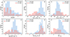 |
Fig. 2. Distribution of physical properties for the radio-quiet (RQ) AGNs (blue histogram) and radio-loud (RL) AGNs (red histogram) used to study the fundamental plane of black hole activity, including: (A) redshift, (B) rest-frame 2–10 keV X-ray luminosity from AGNs (LX), (C) rest-frame 5 GHz radio luminosity from AGNs (LR), (D) the specific star formation rate (sSFR), (E) the black hole mass (MBH) inferred from stellar mass, and (F) the Eddington ratio (λEdd). |
-
(1)
Both the radio-loud and radio-quiet AGN subsamples have a similar redshift range between 0.1 and 4, while the median redshift is 0.9 for the radio-loud AGNs and 1.2 for the radio-quiet AGNs (see panel A of Fig. 2). The p value of the K-S test for the redshift distributions of these two subsamples is about 0.037, which is lower than 0.05. This means that the radio-loud and radio-quiet AGN subsamples have different redshift distributions.
-
(2)
The range of log [LX(erg s−1)] for our radio-quiet AGN sample is between 40.9 and 45.2 with a median of 44.0, while for our radio-loud AGN sample it is between 39.9 and 44.7 with a median of 42.4 (see panel B of Fig. 2). The radio-quiet AGN sample has significantly larger LX than the radio-loud AGN sample. The p value of the K–S test is about 10−16; that is, much lower than 0.05, which indicates a significantly different X-ray luminosity distribution between the radio-loud and radio-quiet AGN subsamples.
-
(3)
The range of log [LR(erg s−1)] for the radio-quiet AGN sample is between 37.9 and 41.5 with a median of 40.0, while for the radio-loud AGN sample it is between 38.4 and 43.4 with a median of 40.5 (see panel C of Fig. 2). The radio-quiet AGN sample has slightly lower LR than the radio-loud AGN sample. The p value of the K–S test is about 0.0006; that is, much lower than 0.05, which indicates a significantly different radio luminosity distribution between the radio-loud and radio-quiet AGN subsamples.
-
(4)
The range of the specific star formation rate (sSFR) for our radio-quiet AGN sample is between 0.001 and 100 Gyr−1 with a median of 0.60 Gyr−1, while for our radio-loud AGN sample it is between 0.003 and 17 Gyr−1 with a median of 0.12 Gyr−1 (see panel D of Fig. 2). Here, the SFR was derived from Paper I, which estimated it with the broadband SED fitting. The radio-quiet AGN sample has a slightly higher sSFR than the radio-loud AGN sample. The p value of the K–S test is about 0.0008; that is, much lower than 0.05, which demonstrates that the radio-loud and radio-quiet AGN subsamples have significantly different sSFRs. This conclusion can also be proved by the different SFG or QG proportions in these two subsamples (see Figure 1 or Section 6.4).
-
(5)
The range of log[MBH/M⊙] for the radio-quiet AGN sample is between 5.35 and 9.62 with a median of 8.36, while for the radio-loud AGN sample it is between 4.28 and 9.70 with a median of 8.58 (see panel E of Fig. 2). The p value of the K–S test is about 0.122; that is, higher than 0.05, which indicates that the radio-loud and radio-quiet AGN subsamples have a similar black hole mass.
-
(6)
The Eddington ratio (λEdd) was defined as λEdd = Lbol/LEdd, where Lbol is the bolometric luminosity and LEdd is the Eddington luminosity. The bolometric luminosity is converted from X-ray luminosity by a bolometric correction factor that is related to the luminosity (e.g., Duras et al. 2020). For our sample, this correction factor was around 20 (Duras et al. 2020). Therefore, here Lbol was calculated by Lbol = LX × 20. The Eddington luminosity was defined as LEdd = 1.3 × 1038MBH/M⊙ in units of erg s−1 (Rybicki & Lightman 1979). The range of λEdd for our radio-quiet AGN sample is between 2.3 × 10⁻⁵ and 51 with a median of 0.06, while for our radio-loud AGN sample it is between 10−5 and 1.0 with a median of 0.001 (see panel F of Fig. 2). The radio-quiet AGN sample has significantly larger λEdd than the radio-loud AGN sample, which is consistent with the negative correlation between radio loudness and the Eddington ratio (e.g., Ho 2002; Panessa et al. 2007; Sikora et al. 2007). The p value of the K-S test is about 10−12; that is, significantly lower than 0.05, which indicates that the radio-loud and radio-quiet AGN subsamples present significantly different Eddington ratios.
5. Fitting the fundamental plane for radio-loud and radio-quiet active galactic nuclei
Following Merloni et al. (2003), we defined the fundamental plane of black hole activity as
 (7)
(7)
where LR is the rest-frame 5 GHz radio luminosity (in units of erg s−1), LX is the rest-frame 2–10 keV X-ray luminosity (in units of erg s−1), and MBH is the black hole mass (in units of M⊙). Then we used the the ordinary least squares (OLS) linear regression method in the Python package SCIKIT-LEARN (Pedregosa et al. 2011) to fit the dataset. Further, we ran the fitting process with 4000 iterations to take the uncertainties of both dependent and independent variables into account. Next, we took the variable LX as an example to show the detailed analysis process. In our sample, the ith object has the observed LX, obs, i with an uncertainty of σi. In the jth fitting process, the value of the variable used for fitting (LX, fit, i, j) was randomly selected from a normal distribution centered at LX, obs, i with a variance of σi. We made the same value selection for the variables LR and MBH. Thus, in the jth fitting process, the ith object had LX, fit, i, j, LR, fit, i, j, and MBH, fit, i, j. After the jth fitting, the best-fit parameters were given as ξX,j ± σX,j, ξM,j ± σM,j, and bj ± σb, j. Finally, fitting with 4000 iterations produced a nearly symmetric distribution for each fitting coefficient. Then we used the mean of the distribution as the best-fit coefficient, while the error was derived from the integrated variance from both fitting process and observed uncertainties. Next, we took the parameter ξX as an example. The best-fit ξX was calculated by  (written as
  hereafter), while its error was calculated by
  . Then we did the same calculation for both ξM and b.
We performed the above fitting process for our radio-quiet and radio-loud AGN samples separately. We found a best-fit fundamental plane of
 (8)
(8)
for the radio-quiet AGN sample, and
 (9)
(9)
for the radio-loud AGN sample. The best-fit coefficients and their errors are summarized in Table 1. The comparison between the observed LR and the predicted LR by the best-fit fundamental plane is shown in Fig. 3. The significantly different fundamental plane between radio-quiet and radio-loud AGNs, and their comparison with literature works, are discussed in detail in Section 6.1. Here, we defined a parameter, σR, to denote the scatter of the observed LR relative to the predicted value from the best-fit fundamental plane. σR for the radio-loud and radio-quiet subsets was 0.37 and 0.39, respectively (see Table 1). We also fit the fundamental plane for the entire radio AGN sample, which shows a much larger scatter with σR = 0.64. Next, we calculated the χ2 and degree of freedom (d.o.f.) for the best-fit results of the entire sample and the two subsets, respectively. Then we used f-test at a confidence level of ≥95% to decide whether splitting the entire sample into the radio-loud and radio-quiet subsets gives different coefficients for the fundamental plane. The f-test p values based on the χ2 and d.o.f. of the entire sample and each subset are all much lower than 0.05. Therefore, these statistical results verify that the radio-loud and radio-quiet AGNs in our sample do follow different fundamental planes. For the radio AGNs with only upper limits for X-ray luminosity, we estimated the lower limits of their radio loudness according to the ratio of LR to LX upper-limits. Therefore, from these sources, we selected 76 radio-loud AGNs with only upper limits for X-ray luminosity based on the previously defined radio-loudness threshold (see Equation (6)). These objects were not included in the regression fitting for the fundamental plane, and they are just shown in Fig. 3 (see the dark red triangles) as a comparison. These radio-loud AGNs are greatly consistent with the fundamental plane (see Equation (9)) obtained with the aforementioned radio-loud AGN sample.
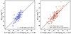 |
Fig. 3. Comparison of the predicted rest-frame 5 GHz luminosity from the best-fit fundamental plane (x axis) and the observed rest-frame 5 GHz luminosity (y axis) for the radio-quiet AGNs (left panel) and the radio-loud AGNs (right panel). The dashed black line in each panel represents the 1:1 line. The empty dark red triangles in the right panel represent the radio-loud AGNs with only upper limits for LX (see parameter calculation in Section 3.3 and see sample selection in Section 5) that were not utilized in the regression fitting for the fundamental plane. |
6. Discussion
The comparison between the best-fit correlation coefficients, ξX and ξM, of the fundamental plane can characterize the accretion physics and origins of X-ray emission for central engines (Merloni et al. 2003). In the ξX–ξM diagram (see Figs. 4, 5, 6), the theoretically predicted correlation coefficients were derived from Merloni et al. (2003). These theoretical models are advection-dominated accretion flow (ADAF; a radiatively inefficient accretion flow; Narayan & Yi 1994; Yuan 2001; Yuan & Narayan 2014, for a review), the synchrotron jet model producing radio emission and X-ray emission by the optically thin synchrotron radiation from jet, and the standard Shakura-Sunyaev disc model (Shakura & Sunyaev 1973; Pringle 1981, for a review). We followed Merloni et al. (2003) in assuming an electron spectral index of p = 2 for all the models, and assumed an accretion efficiency coefficient of q = 2.3 for the ADAF model and q = 1 for the disc model. Next, we give a brief summary of the studies on the fundamental plane in Section 6.1 and further discuss the dependence of the fundamental plane on Eddington ratio (Section 6.2), redshift (Section 6.3), and galaxy star formation properties (Section 6.4). Combining our and literature works, we investigate the central engines of radio-quiet and radio-loud AGNs in Section 6.5.
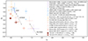 |
Fig. 4. Comparison of the best-fit correlation coefficients, ξX and ξM, of the fundamental plane. Our results for the radio-quiet (RQ) AGNs and radio-loud (RL) AGNs samples are shown as the filled dark red star and the empty dark red star, respectively. The results from literature works are shown as comparisons, including Merloni et al. (2003) (Merloni+2003), Falcke et al. (2004) (Falcke+2004), Plotkin et al. (2012) (Plotkin+2012), Dong et al. (2014) (Dong+2014), Yuan et al. (2009) (Yuan+2009), Gültekin et al. (2009b) (Gültekin+2009), Saikia et al. (2015) (Saikia+2015), Nisbet & Best (2016) (Nisbet & Best 2016), Xie & Yuan (2017) (Xie & Yuan 2017), Bonchi et al. (2013) (Bonchi+2013), Li & Gu (2018) (Li & Gu 2018), Fan & Bai (2016) (Fan & Bai 2016), Wang et al. (2006) (Wang+2006), Li et al. (2008) (Li+2008), and Bariuan et al. (2022) (Bariuan+2022). Purple symbols represent studies based on a sample consisting of both XRBs and local AGNs. Blue symbols represent studies based on LLAGNs. Yellow symbols represent studies for other types of AGNs. Red symbols represent studies for radio-quiet (filled symbols) and radio-loud (empty symbols) AGNs separately. The theoretically predicted correlation coefficients were derived from Merloni et al. (2003) with the electron spectral index p = 2, and are shown as black circles for the ADAF, black triangles for a synchrotron jet model, and black squares for the standard Shakura–Sunyaev disc model. Among them, empty and filled symbols represent the predictions based on a radio spectral index of 0 and −0.5, respectively, and the dashed lines connecting the empty and filled symbols represent the tracks of ξX and ξM due to the variation in the radio spectral index. |
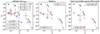 |
Fig. 5. Comparison of the best-fit correlation coefficients, ξX and ξM, of the fundamental plane for Eddington ratio subsamples (A), redshift subsamples (B), and galaxy star formation property subsamples (C). The theoretically predicted correlation coefficients for ADAF, the synchrotron jet model, and the disc model are the same as in Fig. 4, and are shown here as circles, triangles, and squares, respectively. In each panel, filled symbols represent radio-quiet (RQ) AGNs and empty symbols represent radio-loud (RL) AGNs. In panel A, “TW”, “B22”, “D14”, “W06”, and “L08” mean results from this work, Bariuan et al. (2022), Dong et al. (2014), Wang et al. (2006), and Li et al. (2008), respectively. Different colors represent different Eddington ratios: red for |


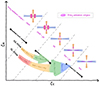 |
Fig. 6. Cartoon illustrating the model for the central engine of radio-quiet AGNs and radio-loud AGNs. Solid black lines represent the theoretically predicted correlation coefficients for ADAF, jet, and standard thin disc models, which are same as Figs. 4 and 5. The upper colored arrow represents the observational results for radio-quiet (RQ) AGNs, while the lower colored arrow represents the observational results for radio-loud (RL) AGNs. The different colors of the arrow represent different Eddington ratios (λEdd) and the direction of the arrow means from low λEdd to high λEdd. The shaded violet regions represent the origins of X-ray emission. The origins of X-ray emission of radio-quiet AGNs at 0.01 < λEdd < 0.1 are consistent with a combination of ADAF and a synchrotron jet model (ADAF+jet model), while at 0.1 < λEdd < 1, they mainly follow the synchrotron jet model (Jet model). The origins of X-ray emission of radio-loud AGNs are consistent with a combination of ADAF and a synchrotron jet model (ADAF+jet model) at λEdd < 0.01, and agree with the synchrotron jet model (Jet model) at 0.01 < λEdd < 0.1, and follow the standard thin disc coupled with a synchrotron jet model (Disc+jet model) at λEdd > 0.1. |
6.1. A brief summary of the fundamental plane studies
Merloni et al. (2003), Falcke et al. (2004), Plotkin et al. (2012), and Dong et al. (2014) all studied the fundamental plane using a sample consisting of both XRBs and local AGNs (see the purple symbols in Fig. 4). The AGN samples of Merloni et al. (2003), Falcke et al. (2004), and Plotkin et al. (2012) mainly focused on low-luminosity AGNs (LLAGNs). Merloni et al. (2003) favor the X-ray emission being produced by an ADAF model, while Falcke et al. (2004) and Plotkin et al. (2012) support the X-ray emission being produced by synchrotron radiation from the inner jet based on a sample having flat or inverted spectra. On the other hand, Dong et al. (2014) showed a significantly different pattern, that their bright AGNs with higher Eddington ratio are in line with the predictions of the disc model. Such a difference indicates that different types of AGNs may have different fundamental planes.
Furthermore, many studies of the fundamental plane only focus on AGNs. Some works studied the fundamental plane of local LLAGNs (Yuan et al. 2009; Gültekin et al. 2009a; Saikia et al. 2015; Nisbet & Best 2016; Xie & Yuan 2017, see blue symbols in Fig. 4). Gültekin et al. (2009a), Saikia et al. (2015), and Nisbet & Best (2016) obtained consistent results with those in Merloni et al. (2003) and Falcke et al. (2004), while Yuan et al. (2009) and Xie & Yuan (2017) exhibited different results. The LLAGN samples in Gültekin et al. (2009a), Saikia et al. (2015), and Nisbet & Best (2016) have a higher Eddington ratio than those in Yuan et al. (2009) and Xie & Yuan (2017), which might explain the different results between them. X-ray-selected AGNs (LX > 1042 erg s−1) from Bonchi et al. (2013) and young radio AGNs from Fan & Bai (2016) show a slight deviation from the ADAF model. Bonchi et al. (2013) mentioned that the deviation is mainly due to the inclusion of the radio upper limits in their analysis, while Fan & Bai (2016) thought that the bad angular resolution of radio data cannot distinguish the extended lobes from the cores, which will result in flatter correlation coefficients. The low-excitation radio-loud AGNs from Li & Gu (2018) show a similar fundamental plane with the LLAGNs (see Fig. 4). The above works usually calculated luminosity assuming a different radio spectral index, which may also bias the fundamental plane.
In addition, many works explore the fundamental plane of radio-quiet and radio-loud populations separately (Wang et al. 2006; Li et al. 2008; Bariuan et al. 2022). Both Wang et al. (2006) and Li et al. (2008) utilized broad-line AGN samples and they got consistent results for the fundamental plane within a 1σ uncertainty (see Fig. 4). They all found that radio-quiet and radio-loud AGNs show quite different fundamental planes. Radio-quiet AGNs favor the ADAF model coupled with a synchrotron jet model, while the radio-loud AGNs favor a combination of the disc model with the synchrotron jet model. More recently, Bariuan et al. (2022) found that for luminous quasars, radio-quiet and radio-loud subsets also have different fundamental planes. Therefore, these works demonstrate that the fundamental plane depends on the radio loudness of AGNs. The rest-frame 5 GHz luminosities of Wang et al. (2006), Li et al. (2008), and Bariuan et al. (2022) were all converted from 1.4 GHz radio flux densities assuming a radio spectral index of −0.5.
We also separately studied the fundamental plane of radio-quiet and radio-loud AGNs. Compared to the literature works (Wang et al. 2006; Li et al. 2008; Bariuan et al. 2022), our samples have a lower X-ray luminosity, lower radio luminosity, and lower Eddington ratio. We also find that there is a different fundamental plane between radio-quiet and radio-loud AGNs. Our low-luminosity radio-quiet AGNs show a slightly different fundamental plane than the high-luminosity radio-quiet AGNs from Wang et al. (2006), Li et al. (2008), and Bariuan et al. (2022), while our low-luminosity radio-loud AGNs present a significantly different result than the high-luminosity radio-loud AGNs from these literature works (see Fig. 4). These results indicate that the fundamental plane may have a dependence on the Eddington ratio (see details in Section 6.2).
The best-fit ξM coefficients of Wang et al. (2006), Li et al. (2008), Fan & Bai (2016), Bariuan et al. (2022), and our results appear relatively small, and fall below the theoretical predications in Fig. 4, especially for the radio-quiet subsamples at a low Eddington ratio (see panel A of Figure 5). The theoretical models shown in Fig. 4 were obtained based on the assumption of p = 2. We calculated the theoretical models with p = 3, but they still cannot explain the observations. Thus, we performed two fitting tests aiming to discuss possible reasons. Firstly, we simultaneously fit the XRBs and LLAGNs from Merloni et al. (2003), our sample, and the quasar sample from Bariuan et al. (2022). The luminosity range of our sample is between the LLAGNs of Merloni et al. (2003) and the quasar sample of Bariuan et al. (2022). The best-fit ξM and ξX are 0.59 ± 0.04 and 0.85 ± 0.03, respectively (σR ∼ 0.7). Next, we only fit the LLAGNs from Merloni et al. (2003), our sample, and the quasar sample from Bariuan et al. (2022). The best-fit ξM and ξX are 0.57 ± 0.07 and 0.86 ± 0.03, respectively (σR ∼ 0.7). Both of these two tests give results consistent with Merloni et al. (2003), which implies that the X-ray emission is produced by the ADAF model. These results differ from those using our sample and the quasar sample (Bariuan et al. 2022), respectively. From a statistical perspective, linear regressions to noisy data with limited dynamic range may result in different coefficients than that with a broad dynamic range (Plotkin et al. 2012). However, given that we use a large sample with a broad luminosity range from LLAGNs to quasars, we do not expect that they follow similar accretion physics and X-ray radiation mechanisms. Therefore, from a scientific perspective, the observational deviation from the theoretical predictions may indicate that some other underlying physical properties have an effect on the fundamental plane.
In addition, other mechanisms may be also responsible for the observational deviation from the theoretical predictions, especially at low Eddington ratios; such as: (1) We only use one solution (i.e., ADAF) of radiatively inefficient flows following Merloni et al. (2003), but we cannot rule out the possibility that other solutions, such as convection-dominated accretion flows, will better explain the observations; (2) Radiatively inefficient flows are prone to produce powerful outflows that may alter the theoretical predictions significantly (Merloni et al. 2003; 3) For the most massive SMBHs (> ∼ 108 M⊙), the synchrotron cooling in jet becomes important, which may bias the fundamental plane (Falcke et al. 2004; Körding et al. 2006; Plotkin et al. 2012). Even so, it is still meaningful to investigate whether other physical properties or processes, such as the Eddington ratio (accretion rate), redshift (cosmic evolution), and galaxy star formation properties (fueling mechanisms) affect the fundamental plane.
6.2. Eddington-ratio dependence of the fundamental plane
We split our radio-quiet AGN subsample into two Eddington-ratio subsets: λEdd ≤ 10−1.5 (with a median value of 0.01) and λEdd > 10−1.5 (with a median value of 0.2). Our radio-loud AGN subsample was split into two Eddington-ratio subsets: λEdd ≤ 10−2.5 (with a median value of 0.0003) and λEdd > 10−2.5 (with a median value of 0.02). The best-fit parameters for the fundamental plane of these subsets and the source number in each subset are summarized in Table 1. The comparison between ξX and ξM is shown in panel A of Fig. 5. For the radio-quiet AGN sample, both the low-Eddington-ratio subset (λEdd ≤ 10−1.5; the filled yellow square in panel A of Fig. 5) and high-Eddington-ratio subset (λEdd > 10−1.5; the filled blue circle in panel A of Fig. 5) agree with an ADAF model coupled with a synchrotron jet model for the origins of X-ray emission. For the radio-loud AGN sample, X-ray emission origins of the low-Eddington-ratio subset (λEdd ≤ 10−2.5; the empty red diamond in panel A of Fig. 5) can be explained by an ADAF model coupled with a synchrotron jet model, while the high-Eddington-ratio subset (λEdd > 10−2.5; the empty yellow square in panel A of Fig. 5) mainly follows a synchrotron jet model. For comparison, ξX and ξM from Wang et al. (2006) (W06), Li et al. (2008) (L08), and Bariuan et al. (2022) (B22) are shown in panel A of Fig. 5. In addition, we also analyzed the fundamental plane for the radio-quiet AGN sample from Dong et al. (2014) (D14) whose best-fit parameters are also shown in panel A of Fig. 5. Our samples and samples from these literature works have different Eddington ratios and follow different fundamental planes (see panel A of Fig. 5). According to these results, we find that for both radio-quiet AGNs and radio-loud AGNs, their fundamental planes may depend on Eddington ratio. We stress that only for our radio-loud and radio-quiet AGN samples does the scatter, σR, not show significant improvement after splitting the sample into two Eddington-ratio subsets (see Table 1), and the f-test p values based on the χ2 and d.o.f. of the entire sample and each Eddington-ratio subset are higher than 0.05. Therefore, only for our samples do the statistical results imply no significant dependence of the fundamental plane on the Eddington ratio, while combining with the quasar samples from previous works, this dependence becomes significant. It demonstrates that using a sample including both low-luminosity and luminous AGNs with a broad Eddington-ratio range is necessary for us to draw a solid conclusion about the dependence of the fundamental plane on the Eddington ratio.
6.3. Redshift dependence of the fundamental plane
We further studied the fundamental plane of radio-quiet and radio-loud AGN subsamples by splitting them into two redshift subsets: 0.1 < z ≤ 1 and 1 < z ≤ 4. For each subset, the best-fit parameters and source numbers are summarized in Table 1. Splitting the radio-loud or radio-quiet AGN sample into two redshift subsets does not reduce the scatter, σR (see Table 1), and produces f-test p values based on the χ2 and d.o.f. higher than 0.05. Therefore, neither the radio-loud AGNs nor the radio-quiet AGNs show a statistically significant redshift dependence of the fundamental plane (also see panel B of Fig. 5). For both radio-loud AGNs and radio-quiet AGNs, there seems to be no significant redshift dependence of the fundamental plane (see panel B of Fig. 5). For luminous AGNs (such as broad-line AGNs and quasars), Li et al. (2008) found no significant dependence on redshift for both radio-quiet and radio-loud subsets across 0 < z < 2.5, while Bariuan et al. (2022) only observed a redshift dependence for radio-loud subsets across 0.1 < z < 5. In the future, larger samples across a broad luminosity range and a wide redshift range are required to draw a firm conclusion about the redshift dependence.
6.4. Galaxy star formation property dependence of the fundamental plane
For the first time, we studied the galaxy star formation property (SFGs and QGs) dependence of the fundamental plane whose best-fit parameters and source numbers are summarized in Table 1. We adopted the UVJ selection criteria in Schreiber et al. (2015) to decide galaxy types (SFG or QG). Here, the UVJ magnitudes of our sample were derived from literature works (GOODS-N: Barro et al. 2019; GOODS-S: Straatman et al. 2016; COSMOS: Weaver et al. 2022). We know that radio AGNs hosted by SFGs and QGs have different cosmic evolutions for the AGN incident rate (e.g., Janssen et al. 2012; Kondapally et al. 2022, Paper I) and radio luminosity functions (Kondapally et al. 2022, Paper I). In addition, SFGs and QGs have different gas contents that may perform different fueling mechanisms toward central SMBHs (e.g., Kauffmann & Heckman 2009; Kondapally et al. 2022; Ni et al. 2023). Therefore, we want to know whether the galaxy star formation properties affect the fundamental plane. For our radio-quiet AGN sample, the scatter, σR, of the QG-hosting subset is significantly lower than that of the entire radio-quiet AGN sample and the SFG-hosting subset (see Table 1), and the f-test comparing the χ2 and d.o.f. of the entire radio-quiet AGN sample and the QG-hosting subset gives a p value much lower than 0.05. We performed the same statistical tests comparing the entire radio-quiet AGNs and the SFG-hosting subset, but the statistical tests do not show significant difference between their fundamental planes. This result can be expected due to the fact that the entire radio-quiet AGN sample is dominated by the SFG-hosting populations (see Table 1). In conclusion, the fundamental plane of the radio-quiet AGNs shows a dependence on the galaxy star formation properties, which means that the disc-jet connection of the radio-quiet AGNs may be related to the fueling mechanisms of their host galaxies. However, for the radio-loud AGN sample, we do not find a statistically significant dependence of the fundamental plane on the galaxy star formation properties: (1) the scatter, σR, is not improved after splitting the radio-loud AGN sample into the SFG- and QG-hosting subsets (see Table 1); and (2) the f-test p value is higher than 0.05. Therefore, the disc-jet connection of the radio-loud AGNs may not be affected by the fueling mechanisms of their host galaxies. In the future, larger samples are required to make more detailed analysis and draw a solid conclusion. In addition, nearly 82% of radio-quiet AGNs are hosted by SFGs and 18% of the radio-quiet AGNs are hosted by QGs (see Table 1 and panel B of Fig. 1), while the fraction of the radio-loud AGNs hosted by SFGs and QGs are both around 50% (see Table 1 and panel C of Fig. 1).
6.5. Central engine for radio-quiet and radio-loud active galactic nuclei
As we mentioned in Section 6.1, radio-quiet AGNs and radio-loud AGNs are found to follow different fundamental planes, which may correspond to different accretion physics and different origins of X-ray radiation for the central engine (see Fig. 4). In Fig. 6, we show a cartoon illustrating the central engines of radio-quiet AGNs and radio-loud AGNs based on the observational results.
According to the observational evidence from our work and literature works (see details in Section 6.2), X-rays emissions of radio-quiet AGNs at 0.01 < λEdd < 0.1 seem to be produced by a combination of ADAF and optically thin synchrotron radiation from the jet, while at 0.1 < λEdd < 1 they are mainly produced by the synchrotron radiation from the jet (see panel A in Fig. 5 or the cartoon illustration in Fig. 6). For radio-quiet AGNs at other λEdd ranges, more observational data are required to verify this trend in the future. Wang et al. (2022a) studied the ambient circumnuclear medium of six radio-quiet AGNs with 0.05 < λEdd < 0.5 based on the high-resolution X-ray analysis for warm absorber outflows. The density profile of the ambient circumnuclear medium shows that for these six radio-quiet AGNs, the accretion physics from 0.01 pc to a few parsec (corresponding to a physical scale from the broad-line region to the torus; Wang et al. 2022b) are consistent with the standard thin disc model. One possible reason for the difference between this work and Wang et al. (2022a) is different physical scales. The fundamental plane describes the disc-jet or corona-jet connection in the innermost region of the accretion flow (Merloni et al. 2003), which reflects the accretion physics around several Schwarzschild radii (e.g., Alston et al. 2020) (corresponding to about 10−4 pc assuming a 108 M⊙ black hole). Thus, the physical scale that we target in this work is much smaller than that in Wang et al. (2022a).
The origins of X-ray emissions of radio-loud AGNs are consistent with a combination of ADAF and a synchrotron jet model at λEdd < 0.01, agree with the synchrotron jet model at 0.01 < λEdd < 0.1, and follow the standard thin disc coupled with a synchrotron jet model at λEdd > 0.1 (see panel A in Fig. 5 or the cartoon illustration in Fig. 6). The result for the high-λEdd radio-loud AGN is consistent with that in Zhong et al. (2024), who found that the extremely powerful radio jets are a result of either the spectral transition from ADAF to a thin disc or a super-Eddington accretion.
7. Summary and conclusions
We investigated the fundamental plane of black hole activity based on a large radio AGN sample selected from the GOODS-N, GOODS-S, and COSMOS/UltraVISTA fields across 0.1 < z ≤ 4. This radio AGN sample consists of 208 objects with available estimates for rest-frame 5 GHz radio luminosity (LR) and rest-frame 2–10 keV X-ray luminosity (LX), and a black hole mass (MBH) inferred from the stellar mass (Section 3). We divided this radio AGN sample into 141 radio-quiet AGNs and 67 radio-loud AGNs (Section 4), and studied their fundamental planes separately (Section 5). Further, we summarized the current studies about the fundamental plane (Section 6.1). Finally, we explored the dependence of the fundamental plane on the Eddington ratio (Section 6.2), redshift (Section 6.3), and galaxy star formation properties (Section 6.4), and discussed the central engines of radio-quiet and radio-loud AGNs (Section 6.5). The main conclusions are shown as follows:
-
(i)
The ratio of LR to LX, also known as a tracer for radio loudness, shows a bimodal distribution that can be described well by two single Gaussian models (Fig. 1). The cross point between these two Gaussian components – that is, log(LR/LX) = − 2.73 – is defined as a radio-loudness threshold to divide radio-quiet and radio-loud AGN in this work.
-
(ii)
Our radio-quiet AGNs have a larger X-ray luminosity, lower radio luminosity, and significantly larger Eddington ratio than our radio-loud AGNs.
-
(iii)
Our radio-quiet and radio-loud AGNs show a significantly different fundamental plane:
 for the radio-quiet AGNs, and
  for the radio-loud AGNs (Fig. 3 and Table 1). Our radio-quiet AGNs can be explained by an ADAF model coupled with a synchrotron jet model, while our radio-loud AGNs mainly agree with a synchrotron-emitting jet model (Fig. 4).
 -
(iv)
For both radio-quiet and radio-loud AGNs, the fundamental plane shows a significant dependence on the Eddington ratio (panel A in Fig. 5), but no significant dependence on redshift (panel B in Fig. 5, respectively). The fundamental plane of radio-quiet AGNs show a dependence on the galaxy star formation properties (SFGs and QGs), while for radio-loud AGNs this dependence disappears.
-
(v)
Radio-quiet and radio-loud AGNs at different accretion states have different fundamental planes (Fig. 4) corresponding to different accretion physics and different origins of X-ray emission (Fig. 6). X-ray emissions of radio-quiet AGNs at 0.01 < λEdd < 0.1 are produced by a combination of ADAF and a synchrotron jet model, while at 0.1 < λEdd < 1 they mainly follow the synchrotron jet model (Fig. 6). The origins of X-ray emission of radio-loud AGNs are consistent with a combination of ADAF and a synchrotron jet model at λEdd < 0.01, agree with the synchrotron jet model at 0.01 < λEdd < 0.1, and follow the standard thin disc coupled with the jet model at λEdd > 0.1 (Fig. 6).
Data availability
All the low-luminosity radio AGNs are summarized in Table A.1, which is available at the CDS via anonymous ftp to cdsarc.cds.unistra.fr (130.79.128.5) or via https://cdsarc.cds.unistra.fr/viz-bin/cat/J/A+A/689/A327
Acknowledgments
We thank the anonymous referee for the constructive comments that greatly improved this paper. We thank Stefano Marchesi and Giorgio Lanzuisi for kind help to access the COSMOS-Legacy survey data. This work is supported by the National Natural Science Foundation of China (Project No. 12173017 and Key Project No. 12141301). LCH was supported by the National Science Foundation of China (11991052, 12011540375, 12233001), the National Key R&D Program of China (2022YFF0503401), and the China Manned Space Project (CMS-CSST-2021-A04, CMS-CSST-2021-A06).
References
- Aird, J., Nandra, K., Laird, E. S., et al. 2010, MNRAS, 401, 2531 [Google Scholar]
- Alberts, S., Rujopakarn, W., Rieke, G. H., Jagannathan, P., & Nyland, K. 2020, ApJ, 901, 168 [NASA ADS] [CrossRef] [Google Scholar]
- Alston, W. N., Fabian, A. C., Kara, E., et al. 2020, Nat. Astron., 4, 597 [NASA ADS] [CrossRef] [Google Scholar]
- Bariuan, L. G. C., Snios, B., Sobolewska, M., Siemiginowska, A., & Schwartz, D. A. 2022, MNRAS, 513, 4673 [NASA ADS] [CrossRef] [Google Scholar]
- Barro, G., Pérez-González, P. G., Cava, A., et al. 2019, ApJS, 243, 22 [NASA ADS] [CrossRef] [Google Scholar]
- Begelman, M. C., Blandford, R. D., & Rees, M. J. 1984, Rev. Mod. Phys., 56, 255 [Google Scholar]
- Bell, E. F., McIntosh, D. H., Katz, N., & Weinberg, M. D. 2003, ApJS, 149, 289 [Google Scholar]
- Bonchi, A., La Franca, F., Melini, G., Bongiorno, A., & Fiore, F. 2013, MNRAS, 429, 1970 [CrossRef] [Google Scholar]
- Boquien, M., Burgarella, D., Roehlly, Y., et al. 2019, A&A, 622, A103 [NASA ADS] [CrossRef] [EDP Sciences] [Google Scholar]
- Burgarella, D., Buat, V., & Iglesias-Páramo, J. 2005, MNRAS, 360, 1413 [NASA ADS] [CrossRef] [Google Scholar]
- Chabrier, G. 2003, ApJ, 586, L133 [NASA ADS] [CrossRef] [Google Scholar]
- Civano, F., Marchesi, S., Comastri, A., et al. 2016, ApJ, 819, 62 [Google Scholar]
- Condon, J. J. 1992, ARA&A, 30, 575 [Google Scholar]
- Cowie, L. L., González-López, J., Barger, A. J., et al. 2018, ApJ, 865, 106 [NASA ADS] [CrossRef] [Google Scholar]
- de Gasperin, F., Intema, H. T., & Frail, D. A. 2018, MNRAS, 474, 5008 [Google Scholar]
- Delhaize, J., Smolčić, V., Delvecchio, I., et al. 2017, A&A, 602, A4 [NASA ADS] [CrossRef] [EDP Sciences] [Google Scholar]
- Delvecchio, I., Daddi, E., Sargent, M. T., et al. 2022, A&A, 668, A81 [NASA ADS] [CrossRef] [EDP Sciences] [Google Scholar]
- Done, C., & Gierliński, M. 2005, MNRAS, 364, 208 [NASA ADS] [CrossRef] [Google Scholar]
- Dong, A.-J., Wu, Q., & Cao, X.-F. 2014, ApJ, 787, L20 [NASA ADS] [CrossRef] [Google Scholar]
- Dubner, G., & Giacani, E. 2015, A&ARv, 23, 3 [Google Scholar]
- Duras, F., Bongiorno, A., Ricci, F., et al. 2020, A&A, 636, A73 [NASA ADS] [CrossRef] [EDP Sciences] [Google Scholar]
- Enia, A., Talia, M., Pozzi, F., et al. 2022, ApJ, 927, 204 [NASA ADS] [CrossRef] [Google Scholar]
- Fabian, A. C. 2012, ARA&A, 50, 455 [Google Scholar]
- Falcke, H., Körding, E., & Markoff, S. 2004, A&A, 414, 895 [NASA ADS] [CrossRef] [EDP Sciences] [Google Scholar]
- Fan, X.-L., & Bai, J.-M. 2016, ApJ, 818, 185 [NASA ADS] [CrossRef] [Google Scholar]
- Gómez-Guijarro, C., Elbaz, D., Xiao, M., et al. 2022, A&A, 658, A43 [NASA ADS] [CrossRef] [EDP Sciences] [Google Scholar]
- Greene, J. E., Strader, J., & Ho, L. C. 2020, ARA&A, 58, 257 [Google Scholar]
- Grimm, H. J., Gilfanov, M., & Sunyaev, R. 2003, MNRAS, 339, 793 [Google Scholar]
- Gültekin, K., Cackett, E. M., Miller, J. M., et al. 2009a, ApJ, 706, 404 [CrossRef] [Google Scholar]
- Gültekin, K., Richstone, D. O., Gebhardt, K., et al. 2009b, ApJ, 698, 198 [Google Scholar]
- Gültekin, K., King, A. L., Cackett, E. M., et al. 2019, ApJ, 871, 80 [Google Scholar]
- Guo, Y., Ferguson, H. C., Giavalisco, M., et al. 2013, ApJS, 207, 24 [NASA ADS] [CrossRef] [Google Scholar]
- Haardt, F., & Maraschi, L. 1991, ApJ, 380, L51 [Google Scholar]
- Helou, G., Soifer, B. T., & Rowan-Robinson, M. 1985, ApJ, 298, L7 [Google Scholar]
- Ho, L. C. 2002, ApJ, 564, 120 [CrossRef] [Google Scholar]
- Ho, L. C. 2008, ARA&A, 46, 475 [Google Scholar]
- Janssen, R. M. J., Röttgering, H. J. A., Best, P. N., & Brinchmann, J. 2012, A&A, 541, A62 [NASA ADS] [CrossRef] [EDP Sciences] [Google Scholar]
- Jin, S., Daddi, E., Liu, D., et al. 2018, ApJ, 864, 56 [Google Scholar]
- Kauffmann, G., & Heckman, T. M. 2009, MNRAS, 397, 135 [NASA ADS] [CrossRef] [Google Scholar]
- Kellermann, K. I., Sramek, R., Schmidt, M., Shaffer, D. B., & Green, R. 1989, AJ, 98, 1195 [Google Scholar]
- King, A., & Pounds, K. 2015, ARA&A, 53, 115 [NASA ADS] [CrossRef] [Google Scholar]
- Kondapally, R., Best, P. N., Cochrane, R. K., et al. 2022, MNRAS, 513, 3742 [NASA ADS] [CrossRef] [Google Scholar]
- Körding, E. 2014, Space Sci. Rev., 183, 149 [CrossRef] [Google Scholar]
- Körding, E., Falcke, H., & Corbel, S. 2006, A&A, 456, 439 [NASA ADS] [CrossRef] [EDP Sciences] [Google Scholar]
- Kroupa, P. 2001, MNRAS, 322, 231 [NASA ADS] [CrossRef] [Google Scholar]
- Lanzuisi, G., Civano, F., Marchesi, S., et al. 2018, MNRAS, 480, 2578 [Google Scholar]
- Lehmer, B. D., Alexander, D. M., Bauer, F. E., et al. 2010, ApJ, 724, 559 [Google Scholar]
- Lehmer, B. D., Basu-Zych, A. R., Mineo, S., et al. 2016, ApJ, 825, 7 [Google Scholar]
- Li, J., Xue, Y., Sun, M., et al. 2019, ApJ, 877, 5 [NASA ADS] [CrossRef] [Google Scholar]
- Li, J. I. H., Shen, Y., Ho, L. C., et al. 2023, ApJ, 954, 173 [NASA ADS] [CrossRef] [Google Scholar]
- Li, S.-L., & Gu, M. 2018, MNRAS, 481, L45 [NASA ADS] [CrossRef] [Google Scholar]
- Li, Z.-Y., Wu, X.-B., & Wang, R. 2008, ApJ, 688, 826 [NASA ADS] [CrossRef] [Google Scholar]
- Liao, M., Gu, M., Zhou, M., & Chen, L. 2020, MNRAS, 497, 482 [NASA ADS] [CrossRef] [Google Scholar]
- Liu, B. F., & Qiao, E. 2022, iScience, 25, 103544 [NASA ADS] [CrossRef] [Google Scholar]
- Liu, T., Tozzi, P., Wang, J.-X., et al. 2017, ApJS, 232, 8 [NASA ADS] [CrossRef] [Google Scholar]
- Liu, D., Daddi, E., Dickinson, M., et al. 2018, ApJ, 853, 172 [Google Scholar]
- Luo, B., Brandt, W. N., Xue, Y. Q., et al. 2017, ApJS, 228, 2 [Google Scholar]
- Lyu, J., Alberts, S., Rieke, G. H., & Rujopakarn, W. 2022, ApJ, 941, 191 [NASA ADS] [CrossRef] [Google Scholar]
- Madau, P., & Dickinson, M. 2014, ARA&A, 52, 415 [Google Scholar]
- Magnelli, B., Ivison, R. J., Lutz, D., et al. 2015, A&A, 573, A45 [NASA ADS] [CrossRef] [EDP Sciences] [Google Scholar]
- Marchesi, S., Lanzuisi, G., Civano, F., et al. 2016, ApJ, 830, 100 [Google Scholar]
- McHardy, I. M., Koerding, E., Knigge, C., Uttley, P., & Fender, R. P. 2006, Nature, 444, 730 [NASA ADS] [CrossRef] [Google Scholar]
- Merloni, A., Heinz, S., & di Matteo, T. 2003, MNRAS, 345, 1057 [Google Scholar]
- Mineo, S., Gilfanov, M., & Sunyaev, R. 2012, MNRAS, 419, 2095 [Google Scholar]
- Mineo, S., Gilfanov, M., Lehmer, B. D., Morrison, G. E., & Sunyaev, R. 2014, MNRAS, 437, 1698 [NASA ADS] [CrossRef] [Google Scholar]
- Murphy, E. J., Momjian, E., Condon, J. J., et al. 2017, ApJ, 839, 35 [Google Scholar]
- Narayan, R., & Yi, I. 1994, ApJ, 428, L13 [Google Scholar]
- Ni, Q., Aird, J., Merloni, A., et al. 2023, MNRAS, 524, 4778 [CrossRef] [Google Scholar]
- Nisbet, D. M., & Best, P. N. 2016, MNRAS, 455, 2551 [NASA ADS] [CrossRef] [Google Scholar]
- Noll, S., Burgarella, D., Giovannoli, E., et al. 2009, A&A, 507, 1793 [NASA ADS] [CrossRef] [EDP Sciences] [Google Scholar]
- Novak, M., Smolčić, V., Delhaize, J., et al. 2017, A&A, 602, A5 [NASA ADS] [CrossRef] [EDP Sciences] [Google Scholar]
- Owen, F. N. 2018, ApJS, 235, 34 [Google Scholar]
- Panessa, F., Barcons, X., Bassani, L., et al. 2007, A&A, 467, 519 [NASA ADS] [CrossRef] [EDP Sciences] [Google Scholar]
- Panessa, F., Baldi, R. D., Laor, A., et al. 2019, Nat. Astron., 3, 387 [Google Scholar]
- Pedregosa, F., Varoquaux, G., Gramfort, A., et al. 2011, J. Mach. Learn. Res., 12, 2825 [Google Scholar]
- Plotkin, R. M., Markoff, S., Kelly, B. C., Körding, E., & Anderson, S. F. 2012, MNRAS, 419, 267 [NASA ADS] [CrossRef] [Google Scholar]
- Pringle, J. E. 1981, ARA&A, 19, 137 [NASA ADS] [CrossRef] [Google Scholar]
- Ruan, J. J., Anderson, S. F., Eracleous, M., et al. 2019, ApJ, 883, 76 [NASA ADS] [CrossRef] [Google Scholar]
- Rybicki, G. B., & Lightman, A. P. 1979, Astron. Quart., 3, 199 [NASA ADS] [CrossRef] [Google Scholar]
- Saikia, P., Körding, E., & Falcke, H. 2015, MNRAS, 450, 2317 [NASA ADS] [CrossRef] [Google Scholar]
- Schreiber, C., Pannella, M., Elbaz, D., et al. 2015, A&A, 575, A74 [NASA ADS] [CrossRef] [EDP Sciences] [Google Scholar]
- Shakura, N. I., & Sunyaev, R. A. 1973, A&A, 24, 337 [NASA ADS] [Google Scholar]
- Sikora, M., Stawarz, Ł., & Lasota, J.-P. 2007, ApJ, 658, 815 [NASA ADS] [CrossRef] [Google Scholar]
- Smolčić, V., Novak, M., Bondi, M., et al. 2017, A&A, 602, A1 [Google Scholar]
- Speagle, J. S., Steinhardt, C. L., Capak, P. L., & Silverman, J. D. 2014, ApJS, 214, 15 [Google Scholar]
- Straatman, C. M. S., Spitler, L. R., Quadri, R. F., et al. 2016, ApJ, 830, 51 [NASA ADS] [CrossRef] [Google Scholar]
- Tadaki, K.-I., Belli, S., Burkert, A., et al. 2020, ApJ, 901, 74 [NASA ADS] [CrossRef] [Google Scholar]
- Terashima, Y., & Wilson, A. S. 2003, ApJ, 583, 145 [Google Scholar]
- Tozzi, P., Gilli, R., Mainieri, V., et al. 2006, A&A, 451, 457 [NASA ADS] [CrossRef] [EDP Sciences] [Google Scholar]
- van der Wel, A., Holden, B. P., Franx, M., et al. 2007, ApJ, 670, 206 [NASA ADS] [CrossRef] [Google Scholar]
- Wang, R., Wu, X.-B., & Kong, M.-Z. 2006, ApJ, 645, 890 [NASA ADS] [CrossRef] [Google Scholar]
- Wang, Y., He, Z., Mao, J., et al. 2022a, ApJ, 928, 7 [NASA ADS] [CrossRef] [Google Scholar]
- Wang, Y., Kaastra, J., Mehdipour, M., et al. 2022b, A&A, 657, A77 [NASA ADS] [CrossRef] [EDP Sciences] [Google Scholar]
- Wang, Y., Wang, T., Liu, D., et al. 2024, A&A, 685, A79 [NASA ADS] [CrossRef] [EDP Sciences] [Google Scholar]
- Weaver, J. R., Kauffmann, O. B., Ilbert, O., et al. 2022, ApJS, 258, 11 [NASA ADS] [CrossRef] [Google Scholar]
- Xie, F.-G., & Yuan, F. 2017, ApJ, 836, 104 [NASA ADS] [CrossRef] [Google Scholar]
- Xue, Y. Q., Luo, B., Brandt, W. N., et al. 2016, ApJS, 224, 15 [Google Scholar]
- Yang, G., Boquien, M., Buat, V., et al. 2020, MNRAS, 491, 740 [Google Scholar]
- Yang, G., Boquien, M., Brandt, W. N., et al. 2022, ApJ, 927, 192 [NASA ADS] [CrossRef] [Google Scholar]
- Yuan, F. 2001, MNRAS, 324, 119 [NASA ADS] [CrossRef] [Google Scholar]
- Yuan, F., & Narayan, R. 2014, ARA&A, 52, 529 [NASA ADS] [CrossRef] [Google Scholar]
- Yuan, F., Yu, Z., & Ho, L. C. 2009, ApJ, 703, 1034 [NASA ADS] [CrossRef] [Google Scholar]
- Zhong, Y., Inoue, A. K., Sugahara, Y., et al. 2024, MNRAS, 529, 4531 [NASA ADS] [CrossRef] [Google Scholar]
All Tables
Best-fitting parameters of the fundamental plane of black hole activity for radio-quiet and radio-loud AGNs in this work.
All Figures
|
Fig. 1. Distribution of the ratio of the rest-frame 5 GHz radio luminosity (LR) to the rest-frame 2–10 keV X-ray luminosity (LX) for the entire final radio AGN sample (panel A), the radio-quiet AGN subsample (panel B), and the radio-loud AGN subsample (panel C). The solid green curve in panel A represents the best-fit model to the entire distribution, which consists of two single Gaussian models (the dash-dotted blue curve and the dotted red curve). The vertical dashed dark gray line in all panels represents the cross point between two single models, which is defined as the radio-loudness threshold to divide radio-loud and radio-quiet AGNs in this work. The vertical dashed light gray line in panel A represents the radio-loudness threshold in Panessa et al. (2007), which was obtained by a sample consisting of local Seyferts and low-luminosity radio galaxies. The blue and red histograms in panel B represent the radio-quiet AGNs hosted by SFGs and QGs, respectively, while in panel C, they represent the radio-loud AGNs hosted by SFGs and QGs, respectively. |
| In the text | |
|
Fig. 2. Distribution of physical properties for the radio-quiet (RQ) AGNs (blue histogram) and radio-loud (RL) AGNs (red histogram) used to study the fundamental plane of black hole activity, including: (A) redshift, (B) rest-frame 2–10 keV X-ray luminosity from AGNs (LX), (C) rest-frame 5 GHz radio luminosity from AGNs (LR), (D) the specific star formation rate (sSFR), (E) the black hole mass (MBH) inferred from stellar mass, and (F) the Eddington ratio (λEdd). |
| In the text | |
|
Fig. 3. Comparison of the predicted rest-frame 5 GHz luminosity from the best-fit fundamental plane (x axis) and the observed rest-frame 5 GHz luminosity (y axis) for the radio-quiet AGNs (left panel) and the radio-loud AGNs (right panel). The dashed black line in each panel represents the 1:1 line. The empty dark red triangles in the right panel represent the radio-loud AGNs with only upper limits for LX (see parameter calculation in Section 3.3 and see sample selection in Section 5) that were not utilized in the regression fitting for the fundamental plane. |
| In the text | |
|
Fig. 4. Comparison of the best-fit correlation coefficients, ξX and ξM, of the fundamental plane. Our results for the radio-quiet (RQ) AGNs and radio-loud (RL) AGNs samples are shown as the filled dark red star and the empty dark red star, respectively. The results from literature works are shown as comparisons, including Merloni et al. (2003) (Merloni+2003), Falcke et al. (2004) (Falcke+2004), Plotkin et al. (2012) (Plotkin+2012), Dong et al. (2014) (Dong+2014), Yuan et al. (2009) (Yuan+2009), Gültekin et al. (2009b) (Gültekin+2009), Saikia et al. (2015) (Saikia+2015), Nisbet & Best (2016) (Nisbet & Best 2016), Xie & Yuan (2017) (Xie & Yuan 2017), Bonchi et al. (2013) (Bonchi+2013), Li & Gu (2018) (Li & Gu 2018), Fan & Bai (2016) (Fan & Bai 2016), Wang et al. (2006) (Wang+2006), Li et al. (2008) (Li+2008), and Bariuan et al. (2022) (Bariuan+2022). Purple symbols represent studies based on a sample consisting of both XRBs and local AGNs. Blue symbols represent studies based on LLAGNs. Yellow symbols represent studies for other types of AGNs. Red symbols represent studies for radio-quiet (filled symbols) and radio-loud (empty symbols) AGNs separately. The theoretically predicted correlation coefficients were derived from Merloni et al. (2003) with the electron spectral index p = 2, and are shown as black circles for the ADAF, black triangles for a synchrotron jet model, and black squares for the standard Shakura–Sunyaev disc model. Among them, empty and filled symbols represent the predictions based on a radio spectral index of 0 and −0.5, respectively, and the dashed lines connecting the empty and filled symbols represent the tracks of ξX and ξM due to the variation in the radio spectral index. |
| In the text | |
|
Fig. 5. Comparison of the best-fit correlation coefficients, ξX and ξM, of the fundamental plane for Eddington ratio subsamples (A), redshift subsamples (B), and galaxy star formation property subsamples (C). The theoretically predicted correlation coefficients for ADAF, the synchrotron jet model, and the disc model are the same as in Fig. 4, and are shown here as circles, triangles, and squares, respectively. In each panel, filled symbols represent radio-quiet (RQ) AGNs and empty symbols represent radio-loud (RL) AGNs. In panel A, “TW”, “B22”, “D14”, “W06”, and “L08” mean results from this work, Bariuan et al. (2022), Dong et al. (2014), Wang et al. (2006), and Li et al. (2008), respectively. Different colors represent different Eddington ratios: red for |
| In the text | |
|
Fig. 6. Cartoon illustrating the model for the central engine of radio-quiet AGNs and radio-loud AGNs. Solid black lines represent the theoretically predicted correlation coefficients for ADAF, jet, and standard thin disc models, which are same as Figs. 4 and 5. The upper colored arrow represents the observational results for radio-quiet (RQ) AGNs, while the lower colored arrow represents the observational results for radio-loud (RL) AGNs. The different colors of the arrow represent different Eddington ratios (λEdd) and the direction of the arrow means from low λEdd to high λEdd. The shaded violet regions represent the origins of X-ray emission. The origins of X-ray emission of radio-quiet AGNs at 0.01 < λEdd < 0.1 are consistent with a combination of ADAF and a synchrotron jet model (ADAF+jet model), while at 0.1 < λEdd < 1, they mainly follow the synchrotron jet model (Jet model). The origins of X-ray emission of radio-loud AGNs are consistent with a combination of ADAF and a synchrotron jet model (ADAF+jet model) at λEdd < 0.01, and agree with the synchrotron jet model (Jet model) at 0.01 < λEdd < 0.1, and follow the standard thin disc coupled with a synchrotron jet model (Disc+jet model) at λEdd > 0.1. |
| In the text | |
Current usage metrics show cumulative count of Article Views (full-text article views including HTML views, PDF and ePub downloads, according to the available data) and Abstracts Views on Vision4Press platform.
Data correspond to usage on the plateform after 2015. The current usage metrics is available 48-96 hours after online publication and is updated daily on week days.
Initial download of the metrics may take a while.