| Issue |
A&A
Volume 689, September 2024
|
|
|---|---|---|
| Article Number | A274 | |
| Number of page(s) | 26 | |
| Section | Numerical methods and codes | |
| DOI | https://doi.org/10.1051/0004-6361/202449609 | |
| Published online | 19 September 2024 | |
Euclid preparation
XLIII. Measuring detailed galaxy morphologies for Euclid with machine learning
1
Institut für Planetologie, Universität Münster,
Wilhelm-Klemm-Str. 10,
48149
Münster,
Germany
Corresponding author; e-mail: This email address is being protected from spambots. You need JavaScript enabled to view it.
2
ESAC/ESA, Camino Bajo del Castillo,
s/n, Urb. Villafranca del Castillo,
28692
Villanueva de la Cañada, Madrid,
Spain
3
Jodrell Bank Centre for Astrophysics, Department of Physics and Astronomy, University of Manchester,
Oxford Road,
Manchester
M13 9PL,
UK
4
Instituto de Astrofísica de Canarias,
Calle Vía Láctea s/n,
38204
San Cristóbal de La Laguna, Tenerife,
Spain
5
Departamento de Astrofísica, Universidad de La Laguna,
38206
La Laguna, Tenerife,
Spain
6
Université PSL, Observatoire de Paris, Sorbonne Université, CNRS, LERMA,
75014,
Paris,
France
7
Université Paris-Cité,
5 Rue Thomas Mann,
75013
Paris,
France
8
INAF-Osservatorio Astronomico di Roma,
Via Frascati 33,
00078
Monteporzio Catone,
Italy
9
INFN section of Naples,
Via Cinthia 6,
80126
Napoli,
Italy
10
Centro de Estudios de Física del Cosmos de Aragón (CEFCA),
Plaza San Juan, 1, planta 2,
44001
Teruel,
Spain
11
Université de Strasbourg, CNRS, Observatoire astronomique de Strasbourg,
UMR 7550,
67000
Strasbourg,
France
12
University of Nottingham,
University Park,
Nottingham
NG7 2RD,
UK
13
SRON Netherlands Institute for Space Research,
Landleven 12,
9747
AD,
Groningen,
The Netherlands
14
Kapteyn Astronomical Institute, University of Groningen,
PO Box 800,
9700
AV
Groningen,
The Netherlands
15
Universität Innsbruck, Institut für Astro- und Teilchenphysik,
Technikerstr. 25/8,
6020
Innsbruck,
Austria
16
School of Computer Science, Merchant Venturers Building, University of Bristol,
Woodland Road,
Bristol,
BS8 1UB,
UK
17
National Astronomical Observatory of Japan,
2-21-1 Osawa,
Mitaka, Tokyo
181-8588,
Japan
18
INAF-Osservatorio Astronomico di Capodimonte,
Via Moiariello 16,
80131
Napoli,
Italy
19
Université Paris-Saclay, CNRS, Institut d’astrophysique spatiale,
91405
Orsay,
France
20
Institute of Cosmology and Gravitation, University of Portsmouth,
Portsmouth
PO1 3FX,
UK
21
INAF-Osservatorio Astronomico di Brera,
Via Brera 28,
20122
Milano,
Italy
22
INAF-Osservatorio di Astrofisica e Scienza dello Spazio di Bologna,
Via Piero Gobetti 93/3,
40129
Bologna,
Italy
23
Dipartimento di Fisica e Astronomia, Università di Bologna,
Via Gobetti 93/2,
40129
Bologna,
Italy
24
INFN-Sezione di Bologna,
Viale Berti Pichat 6/2,
40127
Bologna,
Italy
25
Max Planck Institute for Extraterrestrial Physics,
Giessenbachstr. 1,
85748
Garching,
Germany
26
Universitäts-Sternwarte München, Fakultät für Physik, Ludwig-Maximilians-Universität München,
Scheinerstrasse 1,
81679
München,
Germany
27
INAF – Osservatorio Astrofisico di Torino,
Via Osservatorio 20,
10025
Pino Torinese (TO),
Italy
28
Dipartimento di Fisica, Università di Genova,
Via Dodecaneso 33,
16146,
Genova,
Italy
29
INFN-Sezione di Genova,
Via Dodecaneso 33,
16146,
Genova,
Italy
30
Department of Physics “E. Pancini”, University Federico II,
Via Cinthia 6,
80126,
Napoli,
Italy
31
Instituto de Astrofísica e Ciências do Espaço, Universidade do Porto, CAUP,
Rua das Estrelas,
4150-762
Porto,
Portugal
32
Dipartimento di Fisica, Università degli Studi di Torino,
Via P. Giuria 1,
10125
Torino,
Italy
33
INFN-Sezione di Torino,
Via P. Giuria 1,
10125
Torino,
Italy
34
INAF-IASF Milano,
Via Alfonso Corti 12,
20133
Milano,
Italy
35
Institut de Física d’Altes Energies (IFAE), The Barcelona Institute of Science and Technology, Campus UAB,
08193
Bellaterra (Barcelona),
Spain
36
Port d’Informació Científica, Campus UAB,
C. Albareda s/n,
08193
Bellaterra (Barcelona),
Spain
37
Institute for Theoretical Particle Physics and Cosmology (TTK), RWTH Aachen University,
52056
Aachen,
Germany
38
Dipartimento di Fisica e Astronomia “Augusto Righi” – Alma Mater Studiorum Università di Bologna,
Viale Berti Pichat 6/2,
40127
Bologna,
Italy
39
Institute for Astronomy, University of Edinburgh,
Royal Observatory, Blackford Hill,
Edinburgh
EH9 3HJ,
UK
40
European Space Agency/ESRIN,
Largo Galileo Galilei 1,
00044
Frascati, Roma,
Italy
41
Université Claude Bernard Lyon 1, CNRS/IN2P3,
IP2I Lyon, UMR 5822,
Villeurbanne,
F-69100,
France
42
Institute of Physics, Laboratory of Astrophysics, Ecole Polytechnique Fédérale de Lausanne (EPFL), Observatoire de Sauverny,
1290
Versoix,
Switzerland
43
UCB Lyon 1, CNRS/IN2P3, IUF, IP2I Lyon,
4 rue Enrico Fermi,
69622
Villeurbanne,
France
44
Mullard Space Science Laboratory, University College London, Holmbury St Mary, Dorking,
Surrey
RH5 6NT,
UK
45
Departamento de Física, Faculdade de Ciências, Universidade de Lisboa,
Edifício C8, Campo Grande,
1749-016
Lisboa,
Portugal
46
Instituto de Astrofísica e Ciências do Espaço, Faculdade de Ciências, Universidade de Lisboa,
Campo Grande,
1749-016
Lisboa,
Portugal
47
Department of Astronomy, University of Geneva,
ch. d’Ecogia 16,
1290
Versoix,
Switzerland
48
INAF-Istituto di Astrofisica e Planetologia Spaziali,
via del Fosso del Cavaliere, 100,
00100
Roma,
Italy
49
INFN-Padova,
Via Marzolo 8,
35131
Padova,
Italy
50
Université Paris-Saclay, Université Paris Cité, CEA, CNRS, AIM,
91191
Gif-sur-Yvette,
France
51
School of Physics, HH Wills Physics Laboratory, University of Bristol,
Tyndall Avenue,
Bristol
BS8 1TL,
UK
52
INAF-Osservatorio Astronomico di Trieste,
Via G. B. Tiepolo 11,
34143
Trieste,
Italy
53
Istituto Nazionale di Fisica Nucleare, Sezione di Bologna,
Via Irnerio 46,
40126
Bologna,
Italy
54
INAF – Osservatorio Astronomico di Padova,
Via dell’Osservatorio 5,
35122
Padova,
Italy
55
Institute of Theoretical Astrophysics, University of Oslo,
P.O. Box 1029 Blindern,
0315
Oslo,
Norway
56
Jet Propulsion Laboratory, California Institute of Technology,
4800 Oak Grove Drive,
Pasadena,
CA
91109,
USA
57
Department of Physics, Lancaster University,
Lancaster,
LA1 4YB,
UK
58
von Hoerner & Sulger GmbH,
Schlossplatz 8,
68723
Schwetzingen,
Germany
59
Technical University of Denmark,
Elektrovej 327,
2800
Kgs. Lyngby,
Denmark
60
Cosmic Dawn Center (DAWN),
Denmark
61
Institut d’Astrophysique de Paris, UMR 7095, CNRS, and Sorbonne Université,
98 bis boulevard Arago,
75014
Paris,
France
62
Max-Planck-Institut für Astronomie,
Königstuhl 17,
69117
Heidelberg,
Germany
63
Department of Physics and Helsinki Institute of Physics,
Gustaf Hällströmin katu 2,
00014
University of Helsinki,
Finland
64
Aix-Marseille Université, CNRS/IN2P3, CPPM,
Marseille,
France
65
AIM, CEA, CNRS, Université Paris-Saclay, Université de Paris,
91191
Gif-sur-Yvette,
France
66
Université de Genève, Département de Physique Théorique and Centre for Astroparticle Physics,
24 quai Ernest-Ansermet,
CH-1211
Genève 4,
Switzerland
67
Department of Physics,
PO Box 64,
00014
University of Helsinki,
Finland
68
Helsinki Institute of Physics,
Gustaf Hällströmin katu 2,
University of Helsinki, Helsinki,
Finland
69
European Space Agency/ESTEC,
Keplerlaan 1,
2201
AZ
Noordwijk,
The Netherlands
70
NOVA optical infrared instrumentation group at ASTRON,
Oude Hoogeveensedijk 4,
7991PD
Dwingeloo,
The Netherlands
71
Universität Bonn, Argelander-Institut für Astronomie,
Auf dem Hügel 71,
53121
Bonn,
Germany
72
Aix-Marseille Université, CNRS, CNES, LAM,
Marseille,
France
73
Dipartimento di Fisica e Astronomia “Augusto Righi” – Alma Mater Studiorum Università di Bologna,
via Piero Gobetti 93/2,
40129
Bologna,
Italy
74
Department of Physics, Institute for Computational Cosmology, Durham University,
South Road,
DH1 3LE,
UK
75
Université Côte d’Azur, Observatoire de la Côte d’Azur, CNRS, Laboratoire Lagrange,
Bd de l’Observatoire, CS 34229,
06304
Nice cedex 4,
France
76
Université Paris Cité, CNRS, Astroparticule et Cosmologie,
75013
Paris,
France
77
Institut d’Astrophysique de Paris,
98bis Boulevard Arago,
75014
Paris,
France
78
Department of Physics and Astronomy, University of Aarhus,
Ny Munkegade 120,
DK-8000
Aarhus C,
Denmark
79
Waterloo Centre for Astrophysics, University of Waterloo, Waterloo,
Ontario
N2L 3G1,
Canada
80
Department of Physics and Astronomy, University of Waterloo, Waterloo,
Ontario
N2L 3G1,
Canada
81
Perimeter Institute for Theoretical Physics, Waterloo,
Ontario
N2L 2Y5,
Canada
82
Université Paris-Saclay, Université Paris Cité, CEA, CNRS, Astrophysique, Instrumentation et Modélisation Paris-Saclay,
91191
Gif-sur-Yvette,
France
83
Space Science Data Center, Italian Space Agency, via del Politecnico snc,
00133
Roma,
Italy
84
Centre National d’Etudes Spatiales – Centre spatial de Toulouse,
18 avenue Edouard Belin,
31401
Toulouse Cedex 9,
France
85
Institute of Space Science,
Str. Atomistilor, nr. 409 Măgurele,
Ilfov
077125,
Romania
86
Dipartimento di Fisica e Astronomia “G. Galilei”, Università di Padova,
Via Marzolo 8,
35131
Padova,
Italy
87
Departamento de Física, FCFM, Universidad de Chile,
Blanco Encalada 2008,
Santiago,
Chile
88
Institut d’Estudis Espacials de Catalunya (IEEC), Edifici RDIT, Campus UPC,
08860
Castelldefels, Barcelona,
Spain
89
Institute of Space Sciences (ICE, CSIC), Campus UAB,
Carrer de Can Magrans s/n,
08193
Barcelona,
Spain
90
Satlantis, University Science Park,
Sede Bld
48940,
Leioa-Bilbao,
Spain
91
Centro de Investigaciones Energéticas, Medioambientales y Tecnológicas (CIEMAT),
Avenida Complutense 40,
28040
Madrid,
Spain
92
Infrared Processing and Analysis Center, California Institute of Technology,
Pasadena,
CA
91125,
USA
93
Instituto de Astrofísica e Ciências do Espaço, Faculdade de Ciências, Universidade de Lisboa, Tapada da Ajuda,
1349-018
Lisboa,
Portugal
94
Universidad Politécnica de Cartagena, Departamento de Electrónica y Tecnología de Computadoras,
Plaza del Hospital 1,
30202
Cartagena,
Spain
95
Institut de Recherche en Astrophysique et Planétologie (IRAP), Université de Toulouse, CNRS, UPS, CNES,
14 Av. Edouard Belin,
31400
Toulouse,
France
96
INFN-Bologna,
Via Irnerio 46,
40126
Bologna,
Italy
97
IFPU, Institute for Fundamental Physics of the Universe,
via Beirut 2,
34151
Trieste,
Italy
98
INAF, Istituto di Radioastronomia,
Via Piero Gobetti 101,
40129
Bologna,
Italy
99
Centre de Calcul de l’IN2P3/CNRS,
21 avenue Pierre de Coubertin
69627
Villeurbanne Cedex,
France
100
University of Applied Sciences and Arts of Northwestern Switzerland, School of Engineering,
5210
Windisch,
Switzerland
101
Department of Mathematics and Physics E. De Giorgi, University of Salento,
Via per Arnesano, CP-I93,
73100,
Lecce,
Italy
102
INAF-Sezione di Lecce, c/o Dipartimento Matematica e Fisica, Via per Arnesano,
73100
Lecce,
Italy
103
INFN, Sezione di Lecce, Via per Arnesano,
CP-193,
73100
Lecce,
Italy
104
Institut für Theoretische Physik, University of Heidelberg,
Philosophenweg 16,
69120
Heidelberg,
Germany
105
Université St Joseph; Faculty of Sciences,
Beirut,
Lebanon
106
Junia, EPA department,
41 Bd Vauban,
59800
Lille,
France
107
SISSA, International School for Advanced Studies,
Via Bonomea 265,
34136
Trieste TS,
Italy
108
INFN, Sezione di Trieste,
Via Valerio 2,
34127
Trieste TS,
Italy
109
ICSC – Centro Nazionale di Ricerca in High Performance Computing, Big Data e Quantum Computing,
Via Magnanelli 2,
Bologna,
Italy
110
Instituto de Física Teórica UAM-CSIC, Campus de Cantoblanco,
28049
Madrid,
Spain
111
CERCA/ISO, Department of Physics, Case Western Reserve University,
10900 Euclid Avenue,
Cleveland,
OH
44106,
USA
112
Laboratoire Univers et Théorie, Observatoire de Paris, Université PSL, Université Paris Cité, CNRS,
92190
Meudon,
France
113
Dipartimento di Fisica e Scienze della Terra, Università degli Studi di Ferrara,
Via Giuseppe Saragat 1,
44122
Ferrara,
Italy
114
Istituto Nazionale di Fisica Nucleare, Sezione di Ferrara,
Via Giuseppe Saragat 1,
44122
Ferrara,
Italy
115
Dipartimento di Fisica – Sezione di Astronomia, Università di Trieste,
Via Tiepolo 11,
34131
Trieste,
Italy
116
NASA Ames Research Center, Moffett Field,
CA
94035,
USA
117
Kavli Institute for Particle Astrophysics & Cosmology (KIPAC), Stanford University,
Stanford,
CA
94305,
USA
118
Bay Area Environmental Research Institute, Moffett Field,
California
94035,
USA
119
Department of Astronomy and Astrophysics, University of California, Santa Cruz,
1156 High Street,
Santa Cruz,
CA
95064,
USA
120
Minnesota Institute for Astrophysics, University of Minnesota,
116 Church St SE,
Minneapolis,
MN
55455,
USA
121
Institute Lorentz, Leiden University,
Niels Bohrweg 2,
2333
CA
Leiden,
The Netherlands
122
Institute for Astronomy, University of Hawaii,
2680 Woodlawn Drive,
Honolulu,
HI
96822,
USA
123
Department of Astronomy & Physics and Institute for Computational Astrophysics, Saint Mary’s University,
923 Robie Street,
Halifax, Nova Scotia
B3H 3C3,
Canada
124
Departamento Física Aplicada, Universidad Politécnica de Cartagena, Campus Muralla del Mar,
30202
Cartagena, Murcia,
Spain
125
Department of Computer Science, Aalto University,
PO Box 15400,
Espoo
00 076,
Finland
126
Ruhr University Bochum, Faculty of Physics and Astronomy, Astronomical Institute (AIRUB), German Centre for Cosmological Lensing (GCCL),
44780
Bochum,
Germany
127
Univ. Grenoble Alpes, CNRS, Grenoble INP, LPSC-IN2P3,
53, Avenue des Martyrs,
38000
Grenoble,
France
128
Department of Physics and Astronomy,
Vesilinnantie 5,
20014
University of Turku,
Finland
129
Serco for European Space Agency (ESA), Camino bajo del Castillo s/n, Urbanizacion Villafranca del Castillo, Villanueva de la Cañada,
28692
Madrid,
Spain
130
ARC Centre of Excellence for Dark Matter Particle Physics,
Melbourne,
Australia
131
Centre for Astrophysics & Supercomputing, Swinburne University of Technology,
Victoria
3122,
Australia
132
W.M. Keck Observatory,
65-1120
Mamalahoa Hwy, Kamuela,
HI,
USA
133
Department of Physics and Astronomy, University of the Western Cape, Bellville, Cape Town,
7535,
South Africa
134
Oskar Klein Centre for Cosmoparticle Physics, Department of Physics, Stockholm University,
Stockholm
106 91,
Sweden
135
Astrophysics Group, Blackett Laboratory, Imperial College London,
London
SW7 2AZ,
UK
136
Dipartimento di Fisica, Sapienza Università di Roma,
Piazzale Aldo Moro 2,
00185
Roma,
Italy
137
INFN-Sezione di Roma,
Piazzale Aldo Moro 2, c/o Dipartimento di Fisica, Edificio G. Marconi,
00185
Roma,
Italy
138
Centro de Astrofísica da Universidade do Porto, Rua das Estrelas,
4150-762
Porto,
Portugal
139
Zentrum für Astronomie, Universität Heidelberg,
Philosophenweg 12,
69120
Heidelberg,
Germany
140
Dipartimento di Fisica, Università di Roma Tor Vergata,
Via della Ricerca Scientifica 1,
Roma,
Italy
141
INFN,
Sezione di Roma 2, Via della Ricerca Scientifica 1,
Roma,
Italy
142
Institute of Astronomy, University of Cambridge,
Madingley Road,
Cambridge
CB3 0HA,
UK
143
Department of Astrophysics, University of Zurich,
Winterthurerstrasse 190,
8057
Zurich,
Switzerland
144
Department of Physics and Astronomy, University of California,
Davis,
CA
95616,
USA
145
Department of Astrophysical Sciences, Peyton Hall, Princeton University,
Princeton,
NJ
08544,
USA
146
Niels Bohr Institute, University of Copenhagen,
Jagtvej 128,
2200
Copenhagen,
Denmark
Received:
14
February
2024
Accepted:
19
April
2024
Abstract
The Euclid mission is expected to image millions of galaxies at high resolution, providing an extensive dataset with which to study galaxy evolution. Because galaxy morphology is both a fundamental parameter and one that is hard to determine for large samples, we investigate the application of deep learning in predicting the detailed morphologies of galaxies in Euclid using Zoobot, a convolutional neural network pretrained with 450 000 galaxies from the Galaxy Zoo project. We adapted Zoobot for use with emulated Euclid images generated based on Hubble Space Telescope COSMOS images and with labels provided by volunteers in the Galaxy Zoo: Hubble project. We experimented with different numbers of galaxies and various magnitude cuts during the training process. We demonstrate that the trained Zoobot model successfully measures detailed galaxy morphology in emulated Euclid images. It effectively predicts whether a galaxy has features and identifies and characterises various features, such as spiral arms, clumps, bars, discs, and central bulges. When compared to volunteer classifications, Zoobot achieves mean vote fraction deviations of less than 12% and an accuracy of above 91% for the confident volunteer classifications across most morphology types. However, the performance varies depending on the specific morphological class. For the global classes, such as disc or smooth galaxies, the mean deviations are less than 10%, with only 1000 training galaxies necessary to reach this performance. On the other hand, for more detailed structures and complex tasks, such as detecting and counting spiral arms or clumps, the deviations are slightly higher, of namely around 12% with 60 000 galaxies used for training. In order to enhance the performance on complex morphologies, we anticipate that a larger pool of labelled galaxies is needed, which could be obtained using crowd sourcing. We estimate that, with our model, the detailed morphology of approximately 800 million galaxies of the Euclid Wide Survey could be reliably measured and that approximately 230 million of these galaxies would display features. Finally, our findings imply that the model can be effectively adapted to new morphological labels. We demonstrate this adaptability by applying Zoobot to peculiar galaxies. In summary, our trained Zoobot CNN can readily predict morphological catalogues for Euclid images.
Key words: methods: data analysis / methods: observational / techniques: image processing / galaxies: evolution / galaxies: structure
Corresponding author; e-mail: This email address is being protected from spambots. You need JavaScript enabled to view it.
© The Authors 2024
 Open Access article, published by EDP Sciences, under the terms of the Creative Commons Attribution License (https://creativecommons.org/licenses/by/4.0), which permits unrestricted use, distribution, and reproduction in any medium, provided the original work is properly cited.
This article is published in open access under the Subscribe to Open model. This email address is being protected from spambots. You need JavaScript enabled to view it. to support open access publication.
1 Introduction
Euclid is a space-based mission of the European Space Agency (ESA) launched in 2023. Operating in the optical and near-infrared, its primary goal is to achieve a better understanding of the accelerated expansion of the Universe and the nature of dark matter (Laureijs et al. 2011), and it has a broad range of secondary goals. The Euclid Wide Survey (Euclid Collaboration 2022b) will cover approximately 15 000 deg2 of the extragalactic sky, corresponding to 36% of the celestial sphere. The angular resolution of the Euclid visible imager (VIS, Cropper et al. 2016) of 0.2″ is comparable to that of the Hubble Space Telescope (HST) Advanced Camera for Surveys (ACS), while the field of view of 0.53 deg2 is 175 times larger. Euclid is expected to image billions of galaxies to z ≈ 2 and to a depth of 24.5 mag at 10σ for extended sources (galaxy sizes of ~0.3″) in the VIS band (Laureijs et al. 2011). It will therefore resolve the internal morphology of an unprecedented number of galaxies, estimated at approximately 250 million (Euclid Collaboration 2022a). Many will display complex features, such as clumps, bars, spiral arms, and/or bulges.
Large samples of galaxies with measured detailed morphologies are crucial to understand galaxy evolution and its impact on galaxy structure (Masters 2019). For example, bars are believed to funnel gas inwards from the spiral arms and may lead to the growth of a central bulge (Sakamoto et al. 1999; Masters et al. 2010; Kruk et al. 2018). Euclid will provide an unprecedentedly large dataset of galaxy images with resolved morphology (Euclid Collaboration 2022a), which is essential for studies of galaxy evolution. This includes studying the evolution of morphology with redshift and environment, where Euclid will offer the necessary statistics for analysing trends in stellar mass, colour, and so on, thereby enabling the distinction of complex correlations. However, accurately measuring the morphologies and structures of galaxies will be a challenge.
Numerous methods for diverse applications have been developed to quantify galaxy morphology from imaging data. These include visual classifications (Hubble 1926; de Vaucouleurs 1959; Lintott et al. 2008; Bait et al. 2017), non-parametric morphologies (Conselice 2003; Lotz et al. 2004), galaxy profile fitting (Sérsic 1968; Peng et al. 2002), and machine learning techniques (Huertas-Company et al. 2015; Vega-Ferrero et al. 2021). Many approaches perform measurements in an automated or semi-automated manner, while some facilitate the decomposition of galaxies into multiple constituents, such as bulges and discs, or combine several parameters to scrutinise current models. In a recent study, Euclid Collaboration (2023) compared the performance of five modern morphology fitting codes on simulated galaxies mimicking incoming Euclid images. These galaxies were generated as simplified models with single-Sérsic and double-Sérsic profiles and as neural network-generated galaxies with more detailed morphologies. This Euclid Morphology Challenge was primarily designed to quantify galaxy structures using analytic functions that describe the shape of the surface brightness profile. However, it also highlighted the necessity for additional efforts to fully capture the richness of the detailed morphologies that Euclid will uncover on a larger scale.
For several decades now, expert visual classifications have proven to be successful in measuring detailed morphology (Hubble 1926; de Vaucouleurs 1959; Sandage 1961; van den Bergh 1976; de Vaucouleurs et al. 1991; Baillard et al. 2011; Bait et al. 2017). However, they do not scale well to large surveys and reproducibility is challenging.
The Galaxy Zoo project (Lintott et al. 2008) was set up to harness the collective efforts of thousands of volunteers to classify galaxies from the Sloan Digital Sky Survey (SDSS). With Galaxy Zoo, the number of classified galaxies has significantly increased, with more than 1 million galaxies classified so far. The capability of humans to collectively recognise detailed and faint features in galaxies is unrivalled. However, the number of volunteers on the citizen science platform does not scale well with the sizes of the next generation of surveys, such as those by the Large Synoptic Survey Telescope (LSST, Ivezić et al. 2019) of the Vera Rubin Observatory and by Euclid. Euclid will image more than a billion galaxies (Laureijs et al. 2011). It is unfeasible to classify such a large sample with citizen science alone.
This problem can be solved with machine learning. Machine learning has been shown many times to be a powerful tool for classifying galaxy morphology (Dieleman et al. 2015; Huertas-Company et al. 2015; Domínguez Sánchez et al. 2018, 2019; Cheng et al. 2020; Vega-Ferrero et al. 2021; Walmsley et al. 2022a). Supervised approaches using convolutional neural networks (CNNs) have proven to be effective for this task. Walmsley et al. (2022a) showed that the Galaxy Zoo volunteer responses can be used to train a deep learning model, called Zoobot (Walmsley et al. 2023a), which is able to automatically predict the volunteer labels and therefore the detailed morphologies of galaxies.
The goal of the present study is to evaluate the feasibility of predicting detailed morphologies for emulated Euclid galaxy images with Zoobot and to test the performance. For this, we used emulated Euclid images based on the Cosmic Evolution Survey (COSMOS, Scoville et al. 2007b). We trained Zoobot and assessed its performance on these images using morphology labels provided by volunteers in the Galaxy Zoo: Hubble (GZH, Willett et al. 2017) citizen science project. Ultimately, the goal is to apply Zoobot to the future Euclid galaxy images to generate automated detailed morphology predictions.
This paper is structured as follows: In Sect. 2, the volunteer morphology classifications from GZH and their corresponding HST COSMOS images are introduced. We explain how these images were converted to emulated Euclid images. The Zoobot CNN and the process of fine-tuning is presented in Sect. 3. In Sec. 4, we describe the training of Zoobot for the GZH labels and emulated Euclid images. We also describe the different experiments that we conducted in this study. In Sect. 5, we present and discuss our results. First, we show comparisons of the model trained with different data. We then evaluate the model predictions of the best-performing model in detail. Furthermore, we compare the performance on emulated Euclid images and on the original Hubble images. An example of fine-tuning Zoobot to a new morphology class (finding peculiar galaxies) is presented in Sect. 6. Finally, we summarise our findings and provide an outlook towards the real Euclid images in Sec. 7.
2 Data
In this study, we aim to generate automated detailed morphology predictions on emulated Euclid images, test our pipeline, and evaluate its performance to be able to estimate the quality of future predictions.
To emulate the future Euclid images from existing galaxy images, these need to have at least the same spatial resolution and depth at approximately the same wavelength range as VIS (Cropper et al. 2016). As we are following a supervised deep learning approach, these existing galaxy images need to have reliable morphology labels to train our model and evaluate our results. All these requirements are fulfilled with the COSMOS (Scoville et al. 2007b) galaxy images labelled by volunteers in the GZH (Willett et al. 2017) project.
2.1 Images
2.1.1 Hubble Space Telescope COSMOS images
We used COSMOS galaxy images (Scoville et al. 2007b). For the COSMOS survey, an area of 1.64 deg2 was observed with the ACS Wide Field Channel of HST in the F814W filter with an angular resolution of 0.09″ (Scoville et al. 2007a; Koekemoer et al. 2007). We used the publicly available mosaics in the FITS format with a final drizzle pixel scale of 0.03″. The limiting point source depth at 5σ is 27.2 mag. Therefore, the depth and resolution are better than those estimated for Euclid (24.5 mag at 10σ for sources with ~0.3″ extent and 0.2″, Cropper et al. 2016). The wavelength range of the Euclid VIS band (550–900 nm) includes the F814W band of Hubble. While ideally, data from other HST filters, such as F606W, could be combined to emulate the Euclid VIS observations, the extensive COSMOS survey provides only single-band F814W images. We used the same dataset from COSMOS that was used in GZH (Willett et al. 2017). For the morphological classifications by the volunteers, Willett et al. (2017) applied a magnitude restriction of mI814W < 23.5, yielding a total of 84 954 galaxies.
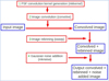 |
Fig. 1 Data pipeline scheme for the emulated Euclid VIS images created as part of the Euclid Data Challenge 2. The green numbers correspond to the numbers of the description of the pipeline given in the text. |
2.1.2 Emulated Euclid COSMOS images
We used available emulated Euclid images generated from the previously described COSMOS images that were created as part of the Euclid Data Challenge 2, with the goal of testing the steps of the data processing for Euclid. The area covered by these images is 1.2° × 1.2°, which is smaller than the original COSMOS field. Therefore, only 76 176 images from the GZH COSMOS set were available. The images are emulated to be Euclid VIS-like and are expected to match the properties of Euclid data, on a reduced scale.
The original HST COSMOS images were rebinned and smoothed to the Euclid pixel scale (0.1″, Laureijs et al. 2011), convolved with a kernel of the difference between the HST ACS and Euclid VIS point spread function (PSF) to emulate the resolution of Euclid (0.2″) and with random Gaussian noise added in order to match the Euclid VIS depth (24.5 mag for galaxy sizes of ~0.3″, Cropper et al. 2016). The emulation software takes as input a high-resolution image (HST COSMOS image in this case) and processes it to emulate a VIS-like image, taking the following steps (see Fig. 1):
First, the software generates an analytical kernel according to the input image PSF of HST ACS and the PSF of the Euclid VIS instrument.
It then convolves the input image according to the previously generated kernel.
Subsequently, it performs the rebinning of the convolved image to the required pixel scale (0.1″).
Finally, Gaussian noise is added to each pixel to reproduce the desired depth in output.
For all galaxies of our dataset, we extracted cutouts from the available emulated Euclid greyscale FITS files with the galaxy in the centre. The sizes of the cutouts were based on the sizes of the galaxies, using three times the Kron radius (3×KRON_RADIUS_HI in Griffith et al. 2012) for each galaxy in order to appear large enough to identify features, but not exceeding the image boundaries. We chose the Kron radius as a measure of galaxy size as it is least sensitive to the galaxy type. With this, the influence of relatively smaller galaxy sizes at higher redshifts on the performance of the network was taken out. The size of the images varies between 10.5″ and 38.3″, with a median of 12.5″. As in Willett et al. (2017), we applied an arcsinh intensity mapping to the images to avoid a saturation of galaxy centres, while increasing the appearance of faint features. We saved the resulting cutouts as 300 × 300 pixel images in the JPG format to reduce the required memory. To conclude, the images have different pixel scales, but approximately the same relative galaxy size compared to the background.
To measure the impact of the lower resolution and noise of the Euclid images on the galaxy classifications, we also created 300 × 300 pixel JPG cutouts for the original HST COSMOS images with an arcsinh intensity mapping. Additionally, we created similar cutouts for the same galaxies imaged by the ground-based Subaru telescope (Kaifu et al. 2000; Taniguchi et al. 2007). To illustrate the effect of the emulation, we show in Fig. 2 example galaxy images with different morphologies (a) from the original HST COSMOS dataset, (b) from the emulated Euclid dataset and (c) from the Subaru dataset. These examples demonstrate that although the morphology is still identifiable, in general, the Euclid images have a lower resolution, potentially leading to different classifications, especially for faint galaxies.
2.2 Volunteer labels
We used the GZH volunteer classifications (Willett et al. 2017) for the same galaxies for which the previously described emulated Euclid images were created. Volunteers on the citizen science project answered a series of questions about the morphology of a set of galaxy images. GZH used COSMOS images with ‘pseudo-colour’. The I814W data was used as an illumination map and the colour information was provided from the BJ, r+, and i+ filters of the Subaru telescope (Griffith et al. 2012). Thus, the galaxy images shown to the volunteers had HST’s angular resolution for the intensity, but the colour gradients were at ground-based resolution. The size of the cutouts corresponded to the galaxy size. Thus, the galaxies had different resolutions but relatively the same size, similar to our emulated Euclid images. An arcsinh intensity mapping was applied before the images were shown as 424 × 424 pixels PNGs to the volunteers.
The series of questions, asked to the volunteers, was structured as a decision tree (Willett et al. 2017) shown in Fig A.1. Some questions were only asked if for the previous question a certain answer was selected. The decision tree was designed similarly to that used in Galaxy Zoo 2 (GZ2, Willett et al. 2013) with some differences, involving questions for clumpiness, as expected for the high-redshift galaxies in the COSMOS dataset. We used the published dataset from Willett et al. (2017), which contains for every galaxy and for every classification the number of volunteers that answered the question and the respective vote fractions for each answer. It also provides metadata, such as photometric redshifts and magnitudes. As mentioned before, the publicly available dataset has a restriction of mI814W < 23.5, meaning that no labels are available for fainter galaxies. We used the GZH volunteer classifications for all available 76176 emulated Euclid galaxy images.
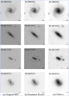 |
Fig. 2 Examples of galaxy images (inverted greyscale) of different morphological types (image IDs 20092952, 20172737, 20177553, 20107313): (a) from the original HST COSMOS dataset, (b) from the emulated Euclid VIS dataset, and (c) from the Subaru dataset. The images are scaled with galaxy size using three times the Kron radius. The black bars represent a length of 1″. The image IDs are the unique identifiers for the galaxies of the COSMOS survey (Griffith et al. 2012). |
3 Zoobot
The newly developed and publicly released Python package Zoobot (Walmsley et al. 2023a) is a CNN trained for predicting detailed galaxy morphology, such as bars, spiral arms, and discs. In this section, we describe the Zoobot CNN and how we adapted it to the emulated Euclid images with the corresponding GZH volunteer labels.
3.1 Bayesian neural network: Zoobot
Zoobot was initially developed to automatically predict detailed morphology for Dark Energy Camera Legacy Survey (DECaLS) (Dey et al. 2019) DR5 galaxy images (Walmsley et al. 2022a). It was trained on the corresponding volunteer classifications from the Galaxy Zoo: DECaLS (GZD) GZD-5 campaign. The 249 581 GZD-5 volunteer classifications were used for training Zoobot on the questions in the GZD-5 decision tree. The volunteer responses for the different questions had different uncertainties, depending on how many volunteers answered a question for a specific galaxy image.
The Bayesian Zoobot CNN learns from all volunteer responses while taking the corresponding uncertainty into account (Walmsley et al. 2022a). Thus, all GZD-5 galaxies could be included in the training. Zoobot was trained on all classification tasks (all questions of the GZD-5 decision tree) simultaneously, leading to shared representations of the galaxies and to increased performance for all tasks. The base architecture of Zoobot is the EfficientNet B0 model (Tan & Le 2019) with a modified final output layer (Walmsley et al. 2022a). The layer consists of one output unit per answer of the decision tree, giving predictions between 1 and 100 using softmax or sigmoid activation. Zoobot does not predict discrete classes, but Dirichlet-Multinomial posteriors that can be transformed into predicted vote fractions. This is achieved by using a Dirichlet-Multinomial loss function for each question q
![Mathematical equation: $\[\mathcal{L}_q=\sum_q \int \operatorname{Multinomial}\left(\boldsymbol{k}_q {\mid} \boldsymbol{\rho}, N_q\right) \operatorname{Dirichlet}(\boldsymbol{\rho} {\mid} \boldsymbol{\alpha}) d \boldsymbol{\rho},\]$](/articles/aa/full_html/2024/09/aa49609-24/aa49609-24-eq1.png) (1)
(1)
with the total number of responses Nq to the question q, kq the ground truth number of votes for each answer, and ρ the probabilities of a volunteer giving each answer. The model predicts the Dirichlet parameters α = fq to the answers measured via the values of the output units of the final layer. Each vector has one element per answer. The integral is analytic as Multinomial and Dirichlet distributions are conjugates. The loss is then applied by summing over all questions of the decision tree
![Mathematical equation: $\[\ln \mathcal{L}=\sum_q \mathcal{L}_q,\]$](/articles/aa/full_html/2024/09/aa49609-24/aa49609-24-eq2.png) (2)
(2)
with the assumption that answers to different questions are independent. The loss naturally handles volunteer votes with different uncertainties (different number of responses), as, for example, questions with no answers do not influence the gradients in training, since ∂Lq(kq = 0, Nq = 0, α)/∂α = 0. We refer the reader to Walmsley et al. (2022a) and Walmsley et al. (2022c) for further details.
Zoobot is therefore well suited for our goal of automatically predicting detailed morphology for Euclid galaxy images. With Zoobot, we can train on all available emulated Euclid galaxies with their GZH labels, since it takes the uncertainty of the volunteer answers into account. We have to train only one model for all galaxy morphology types, since Zoobot is trained on all questions simultaneously. Rather than just discrete classifications, we generate posteriors.
3.2 Transfer learning
The trained Zoobot models can be adapted (‘fine-tuned’) to solve a new task for galaxy images (Walmsley et al. 2023a). This adaption of a previously trained machine learning model to a new problem is called transfer learning (Lu et al. 2015). Instead of retraining all model parameters, the original model architecture and the corresponding parameters (weights) learned from the previous training can be reused. Far fewer new labels for the same performance are required using transfer learning compared to training from scratch (Domínguez Sánchez et al. 2019; Walmsley et al. 2022b). In Walmsley et al. (2022b) the adaption of Zoobot to the new problem of finding ring galaxies is described. The pretrained Zoobot models outperformed models built from scratch, especially when the number of images involved in the training was limited. Pretraining on all GZD-5 tasks, involving the usage of shared representations, also leads to higher accuracy for finding ring galaxies than pretraining on only a single task.
In Walmsley et al. (2022c) the GZ-Evo dataset was introduced, which is a combined dataset from all major Galaxy Zoo campaigns. The included campaigns were Galaxy Zoo 2 (GZ2, Willett et al. 2013) trained on galaxy images from the Sloan Digital Sky Survey (SDSS) Data Release 7, Galaxy Zoo: CANDELS (GZC, Simmons et al. 2017) trained on galaxy images from the Cosmic Assembly Near-infrared Deep Extragalactic Legacy survey (CANDELS) also involving HST images (Grogin et al. 2011), and the previously described GZD-5 (Walmsley et al. 2022a) and GZH (Willett et al. 2017). Additionally, Galaxy Zoo labels from the Mayall z-band Legacy Survey (MzLS) and the Beijing-Arizona Sky Survey (BASS, Dey et al. 2019) were used, which are part of Galaxy Zoo DESI (Walmsley et al. 2023b). Zoobot was trained on all 206 possible morphology classifications of the different campaigns simultaneously, with the involved Dirichlet loss naturally handling unknown answers from different decision trees (Walmsley et al. 2022c). Pretraining with GZ-Evo shows further improvements for the task of finding ring galaxies compared to direct training. With training from different campaigns, Walmsley et al. (2022c) hypothesise that because the model was trained on all galaxy images from different campaigns (having different redshifts and magnitudes) and on all possible questions, the model builds a galaxy representation of high generalization. Therefore, we expect this model to be best suited to be adapted to our new tasks.
We thus used a version of Zoobot pretrained on a modified GZ-Evo catalogue, specifically pretrained on all major Galaxy Zoo campaigns with the exception of GZH in order to not influence our results when training to the GZH decision tree. In total, 450000 galaxy images with volunteer classifications were involved in the pretraining. We also conducted experiments with versions of Zoobot pretrained with different datasets (pretrained on GZD-5 galaxies and without pretraining). The results for these models are presented in Appendix B. We adapted the pretrained Zoobot model to our new problem. This involved two new tasks simultaneously: (i) training on new images, namely the emulated Euclid VIS images, and (ii) training on a new decision tree.
4 Training
In this section, we describe how we used the GZH volunteer labels to train Zoobot (Sec. 4.1). Furthermore, we describe the experiments we conducted for the training, that is, restricting the magnitude and number of examples used for training (Sec. 4.2). Lastly, we present how each model was trained in more detail (Sec. 4.3).
4.1 Preparing the datasets
Unlike the GZD-5 decision tree used in Walmsley et al. (2022a), the GZH decision tree incorporates questions that have multiple possible answers, although not all leading to the same subsequent question (see Fig. A.1 and Willett et al. 2017). Since Zoobot does not support this type of structure, we simply excluded the subsequent questions associated with such cases. The remaining questions and their corresponding answers used in this study can be found in Table 1. Moreover, similar to Walmsley et al. (2022a), we used the raw vote counts as we fine-tuned previously trained Zoobot models that have already been trained on the raw vote counts. Moreover, the used Dirichlet-Multinomial loss (see Eq. (1)) is statistically only valid when using raw vote counts. Assessing Zoobot’s performance when considering votes weighted by user performance or debiased for observational effects is beyond the scope of this research.
Additionally, we provide the average number of volunteer responses for each question in Table 1. Furthermore, we list the fraction frel of galaxies for which the question is deemed relevant. We define a galaxy to be relevant for a specific question when at least half of the volunteers answered that question (for example measuring the number of spiral arms is only meaningful if the majority of volunteers classified the galaxy as spiral in the previous question), similar to the approach taken by Walmsley et al. (2022a). Since every volunteer responded to the initial question of ‘smooth-or-featured’, this question has the highest number of responses. However, with the exception of the ‘how-rounded’ question, all subsequent questions were asked only if the answer to the first question was ‘featured’. Consequently, the number of responses decreases substantially as one progresses in the decision tree, resulting in greater uncertainty. As previously mentioned, Zoobot is able to learn from uncertain volunteer responses.
Our dataset contains 76 176 greyscale galaxy images with detailed morphology labels. This dataset, referred to as the ‘complete set’, encompasses all available images. It has a magnitude range of 10.5 < mI814W < 23.5 and a redshift range of 0 < z < 4.1. In order to ensure an unbiased evaluation of the model, we divided this set into two distinct subsets: one for training and validation, and another independent test set for evaluation purposes. To accomplish this, we performed a random split of 80% for training and validation, and the remaining 20% for the test set. Subsequently, we further split the training and validation set using another random 80/20 percent split. The resulting datasets are listed in Table 2.
Questions and corresponding answers from GZH used for training Zoobot.
4.2 Experiments
The Euclid mission is anticipated to generate an unparalleled number of galaxy images with approximately 250 million having resolved internal morphology (Euclid Collaboration 2022a), but humans will only have limited capacity to label them. Consequently, it is important to assess the number of labelled galaxies required to achieve satisfactory performance in morphology predictions (Sect. 4.2.1). Additionally, we aim to investigate the selection criteria for which galaxies to label (Sect. 4.2.2). Suppose a person has the capacity to label 1000 galaxy images. An open question is whether the automated predictions will get better if those 1000 galaxies are selected randomly, or if 1000 bright galaxies are used instead.
Datasets of Euclid images with GZH labels used in this study.
4.2.1 Restricting the training set size
Our goal is to assess the performance of Zoobot based on a limited number of galaxies used for training. Hence, we randomly chose a specific number Ntrain of galaxy images from the training and validation sets (refer to Table 2). These selected images were then used for training. To ensure a fair comparison between all models, we consistently evaluated the performance on the complete test set, without excluding any images.
4.2.2 Restricting the magnitude
Typically, assessing the morphology of brighter galaxies is more straightforward compared to fainter ones. Our goal here is to investigate whether our automated morphology predictions have a better performance when trained on bright galaxies or on randomly selected galaxies from the complete dataset, especially when the number of examples is limited. We therefore created, from our complete training and validation set, a subset which we refer to as the ‘bright set’, by applying a magnitude restriction of mI814W < 22.5. This resulted in a bright training and validation set comprising 27 882 images. Similar to the complete set, we then performed an 80/20 percent split for training and validation purposes (see Table 2).
4.3 Training Zoobot
We used the TensorFlow (Abadi et al. 2016) implementation of Zoobot (Walmsley et al. 2023a). We trained Zoobot on the datasets shown in Table 2 by using the fine-tuning procedure described in the code of Walmsley et al. (2023a). For this, we replaced the original model head with a single dense layer with the number of neurons corresponding to the number of GZH answers used, specifically 40 neurons for 40 answers to 13 questions (see Table 1). As in Walmsley et al. (2022c), we selected the sigmoid activation function for the final layer to predict scores between 1 and 100 corresponding to the Dirichlet parameters (see Eq. (1)). The JPG images with the applied arcsinh intensity mapping (see Sect. 2.1.2) were normalised to values between 0 and 1 before feeding them into the network. Additionally, we applied similar augmentations as Walmsley et al. (2022a) to all images during training, namely a random vertical flip of the image with a probability of 0.5 and a rotation by a random angle. As in the code of Walmsley et al. (2023a), the training process was divided into two parts: at first, we only trained the new head, and in a second step the entire model, as soon as the validation loss was not decreasing for more than 20 consecutive epochs. Furthermore, we reduced the learning rate by a factor of 0.25 when the validation loss did not decrease for ten consecutive epochs. The chosen hyperparameters were selected as they lead to the best model performance in comparison to multiple other tested values. We used the Adam optimizer (Kingma & Ba 2015) for training. We trained the pretrained model with the bright and complete training sets with different numbers of images ranging between five and all the available images (see Table 2). To evaluate how Euclid’s lower resolution and noise affect the performance of our model, we conducted separate training using the original HST COSMOS images for the same set of galaxies (see Sect. 2). This approach allows us to analyse the impact independently of training with a new decision tree.
5 Results: Zoobot for Euclid images
We trained Zoobot to emulated Euclid VIS images with GZH labels. In Sect. 5.1, we compare the various models trained in this study, which were trained with different numbers of images from the bright or complete sets. We then evaluate the model with the best performance on Euclid images in detail in Sect. 5.2.
5.1 Comparing models – The impact of the number of training galaxies and magnitude restriction
Zoobot is not predicting discrete classes, but rather posteriors that can be converted into vote fractions (values between 0 and 1). This is accomplished by dividing the predicted Dirichlet parameter for a particular answer by the sum of the parameters of all answers to the corresponding question. To evaluate the performance of Zoobot, we used the predicted vote fractions and compared them with the corresponding volunteer vote fractions (considered to be ‘ground truth’ vote fractions). This allows for a comprehensive assessment of Zoobot’s performance. To ensure the inclusion of only relevant galaxies for a specific question, we considered galaxies for which at least half of the volunteers provided an answer (see Table 1). Following the method described in Walmsley et al. (2022a), for a given answer i to a morphology question j, we calculated the absolute difference between the predicted vote fraction fpred and the volunteer vote fraction fgt for each relevant galaxy in the test set. We then averaged these differences over all relevant galaxies nj as
![Mathematical equation: $\[\delta_i:=\overline{\left|f_{\text {pred }}-f_{\text {gt }}\right|}.\]$](/articles/aa/full_html/2024/09/aa49609-24/aa49609-24-eq3.png) (3)
(3)
To allow for easier comparison among different models, while considering the performance on all answers, we calculated the unweighted average of all Sδi values. This aggregated measure, referred to as the averaged vote fraction mean deviation ![Mathematical equation: $\[\bar{\delta}\]$](/articles/aa/full_html/2024/09/aa49609-24/aa49609-24-eq4.png) served as our primary metric for comparison, with lower values indicating better performance. For consistency, we evaluated the models using predictions on the same complete test set consisting of 15236 images (see Table 2).
served as our primary metric for comparison, with lower values indicating better performance. For consistency, we evaluated the models using predictions on the same complete test set consisting of 15236 images (see Table 2).
5.1.1 Overview
We show in Fig. 3 the model performance (given by the averaged mean vote fraction deviations ![Mathematical equation: $\[\bar{\delta}\]$](/articles/aa/full_html/2024/09/aa49609-24/aa49609-24-eq5.png) ) depending on the number of training galaxy images used, Ntrain, for the models trained on galaxies from the bright and complete set. The figure summarises our experiments with different magnitude restrictions and number of training images.
) depending on the number of training galaxy images used, Ntrain, for the models trained on galaxies from the bright and complete set. The figure summarises our experiments with different magnitude restrictions and number of training images.
As expected, with increasing number of training galaxies, the average mean deviation ![Mathematical equation: $\[\bar{\delta}\]$](/articles/aa/full_html/2024/09/aa49609-24/aa49609-24-eq7.png) is decreasing: the more galaxy examples (of different types) are used for training, the better the model predictions get for all answers. Notably, no substantial discrepancies are observed between training on bright galaxies or randomly selected galaxies from the complete set. The model trained on all available galaxy images from the complete set yields the best performance, characterised by the lowest
is decreasing: the more galaxy examples (of different types) are used for training, the better the model predictions get for all answers. Notably, no substantial discrepancies are observed between training on bright galaxies or randomly selected galaxies from the complete set. The model trained on all available galaxy images from the complete set yields the best performance, characterised by the lowest ![Mathematical equation: $\[\bar{\delta}\]$](/articles/aa/full_html/2024/09/aa49609-24/aa49609-24-eq8.png) of approximately 9.5% (analysed in Sect. 5.2).
of approximately 9.5% (analysed in Sect. 5.2).
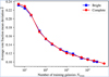 |
Fig. 3 Vote fraction mean deviation averaged over all morphology answers |
![Mathematical equation: $\[\bar{\delta}\]$](/articles/aa/full_html/2024/09/aa49609-24/aa49609-24-eq6.png)
5.1.2 Zoobot trained on only 1000 galaxy images
Next, we compared the model performance in more detail for the models trained on 1000 galaxies from the bright and complete set. Fig. 4 shows the vote fraction mean deviations δi for all morphology answers i for both models. We selected 1000 galaxies as a reasonably small quantity that a single expert could potentially label, while still achieving satisfactory performance for most questions.
All answers reach a mean deviation below 22% indicating that training with only 1000 galaxies already leads to high model performance in general. For most answers, there is no substantial difference between training on bright or complete galaxies.
In particular, for the ‘disc-edge-on’ and ‘bar’ questions, the model shows approximately the same performance when trained on either 1000 bright or 1000 random galaxies. Thus, the relevant features that the model learns do not change qualitatively with different magnitudes. Additionally, the ‘disc-edge-on’ task seems to be easier to learn because the deviations δi are well below 10%.
For the ‘clumpy-appearance’, ‘galaxy-symmetrical’ and ‘clumps-embedded’ questions, Zoobot performs slightly better (by about 1%) when trained on random galaxies from the complete set than when trained on bright galaxies. The better performance for these clump-related questions can thus be explained with the higher number of relevant examples in the complete training set compared to the bright set, as clumpiness is more frequent among fainter galaxies. On the other hand, identifying spiral arms seems to be more effective (by about 2%) when training on bright galaxies. This suggests that the examples included in the bright training set provide clearer and more reliable labels to learn to identify spiral arms.
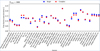 |
Fig. 4 Vote fraction mean deviations δi of the model predictions and the volunteer labels for the different morphology answers i (see Eq. (3)), for models trained on 1000 bright or random galaxies from the complete set. Lower δi indicates better performance. |
5.1.3 Number of training galaxies for different morphology types
Figure 5 shows the dependence of the model performance (vote fraction mean deviation ![Mathematical equation: $\[\bar{\delta}\]$](/articles/aa/full_html/2024/09/aa49609-24/aa49609-24-eq9.png) j) on the number of training galaxies Ntrain for the different morphology questions j. Here, the vote fraction mean deviation is provided as the average of all answers for a particular morphology question and the models were trained on galaxies randomly selected from the complete set.
j) on the number of training galaxies Ntrain for the different morphology questions j. Here, the vote fraction mean deviation is provided as the average of all answers for a particular morphology question and the models were trained on galaxies randomly selected from the complete set.
An increase in the number of training galaxies generally leads to improved performance, characterised by a decrease in the vote fraction mean deviation. This means that in general for all morphology tasks, performance can be improved with training on more labelled examples. All questions reach an averaged vote fraction mean deviation below 12% (highlighted in Fig. 5) when trained with all available galaxies from the complete set. They show different dependencies on the number of training galaxies.
Although in general more training examples increase the quality of the predictions, there are instances where a larger number of galaxies leads to slightly worse performance. These fluctuations in vote fraction mean deviation are particularly noticeable in the low-number regime, for example for the ‘how-rounded’ question with 200 training galaxies. They can be attributed to the model’s sensitivity to the specific galaxies randomly selected for training. Nevertheless, these variations do not alter the overall observable trends for the different questions.
When comparing the various questions, the ‘disc-edge-on’ task not only has the lowest mean deviation (as discussed in Sect. 5.2) when trained with the complete set, but it also achieves a deviation below 10% after training with just 100 galaxies. This is even more impressive as only 6.1% of the galaxies are relevant (see Table 1), although Zoobot learns from all galaxies. This further indicates that identifying disc galaxies is easier to learn than other tasks of the decision tree. Similarly for the ‘bulge-size’ question, the model achieves a deviation below 12% after training with only 100 images. Since these tasks were included in all GZ decision trees, this outcome can be interpreted as a demonstration of the effectiveness of fine-tuning. Furthermore, training on only 100 random galaxies leads for the ‘smooth-or-featured’ question to deviations below 12%. This question was included in all GZ decision trees as the first question and was thus answered by all volunteers, and therefore required fewer new examples compared to other tasks.
In contrast, for the ‘has-spiral-arms’ question, 60000 galaxies are required to achieve deviations below 12%. Despite the inclusion in all GZ decision trees, a substantial number of examples are still necessary to accurately predict the corresponding vote fractions. This observation suggests that detecting spiral arms might pose a greater challenge for Euclid images compared to the galaxies in the pretraining datasets. Additionally, questions related to clumps in galaxies exhibit similar patterns, requiring a range of 10 000 to 60 000 random galaxies to achieve a deviation below 12%. From the campaigns involved in the pretraining of Zoobot, these clump-related questions were exclusively included in the GZC campaign. Consequently, the impact of this pretraining is likely less effective for these tasks. Moreover, given that spiral arms and clumps involve finer structures, the associated tasks are inherently more complex and need a larger number of training examples.
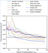 |
Fig. 5 Vote fraction mean deviations of the model predictions |
![Mathematical equation: $\[\bar{\delta}\]$](/articles/aa/full_html/2024/09/aa49609-24/aa49609-24-eq10.png)
5.2 Analysis of the best performing model
In this section, we analyse the performance of Zoobot for emulated Euclid VIS images with the lowest averaged vote fraction mean deviation ![Mathematical equation: $\[\bar{\delta}\]$](/articles/aa/full_html/2024/09/aa49609-24/aa49609-24-eq11.png) , and thus the best performing model, as derived in Sect. 5.1. We show examples of Zoobot’s output, then investigate the performance with standard classification metrics after discretizing the vote fractions (Sect. 5.2.1) and demonstrate how our model can be used to find spiral galaxies in a given dataset (Sect. 5.2.2). Next, we analyse the predicted vote fractions directly by looking at the mean (Sect. 5.2.3) and the histograms (Sect. 5.2.4) of the deviations from their respective volunteer vote fractions, and by investigating their redshift and magnitude dependence (Sect. 5.2.5). Finally, we compare the model performance between HST and Euclid images (Sect. 5.2.6).
, and thus the best performing model, as derived in Sect. 5.1. We show examples of Zoobot’s output, then investigate the performance with standard classification metrics after discretizing the vote fractions (Sect. 5.2.1) and demonstrate how our model can be used to find spiral galaxies in a given dataset (Sect. 5.2.2). Next, we analyse the predicted vote fractions directly by looking at the mean (Sect. 5.2.3) and the histograms (Sect. 5.2.4) of the deviations from their respective volunteer vote fractions, and by investigating their redshift and magnitude dependence (Sect. 5.2.5). Finally, we compare the model performance between HST and Euclid images (Sect. 5.2.6).
To verify the quality of the predictions, four examples of Zoobot’s output on different galaxies from the complete test set are shown in Fig. 6. The selected answer for every question is the one with the highest predicted vote fraction, while the asked questions follow the structure of the GZH decision tree (see Table 1 and Fig. A.1). Figure 7 shows four galaxies from the complete test set with the highest predicted vote fractions for five example answers – (a) spiral, (b) completely rounded, (c) disc, (d) bar, and (e) clumpy – in order to demonstrate the quality of Zoobot’s predictions.
5.2.1 Discrete classifications
To get an intuitive sense of Zoobot’s performance for the different morphology tasks, we converted the predicted vote fractions into discrete values by binning them to the class with the highest predicted vote fraction. However, it is important to note that these metrics only provide a basic indication of Zoobot’s performance and do not fully capture its ability to predict morphology, as the information is simplified and reduced.
We evaluated the discretised predictions with standard classification metrics for the different classes. Accuracy A is the fraction of correct predictions for both the positive and negative class among the total number of galaxy images Ntotal. It is calculated as
![Mathematical equation: $\[A=\frac{N_{\mathrm{TP}}+N_{\mathrm{TN}}}{N_{\text {total }}},\]$](/articles/aa/full_html/2024/09/aa49609-24/aa49609-24-eq12.png) (4)
(4)
where NTP is the number of true positives and NTN the number of true negatives.
Precision P is the fraction of correct classifications among the galaxies predicted to belong to a particular class. It is calculated as
![Mathematical equation: $\[P=\frac{N_{\mathrm{TP}}}{N_{\mathrm{TP}}+N_{\mathrm{FP}}},\]$](/articles/aa/full_html/2024/09/aa49609-24/aa49609-24-eq13.png) (5)
(5)
where NFP is the number of false positives.
Recall R is defined as the fraction of correct classifications among the galaxies of a certain class and calculated as
![Mathematical equation: $\[R=\frac{N_{\mathrm{TP}}}{N_{\mathrm{TP}}+N_{\mathrm{FN}}},\]$](/articles/aa/full_html/2024/09/aa49609-24/aa49609-24-eq14.png) (6)
(6)
where NFN is the number of false negatives.
The F1-score combines precision and recall by taking their harmonic mean. Thus, it is a more general measure for evaluating model performance. It is calculated as
![Mathematical equation: $\[F_1=2 \frac{P R}{P+R}.\]$](/articles/aa/full_html/2024/09/aa49609-24/aa49609-24-eq15.png) (7)
(7)
All of these metrics have values between 0 and 1. Some classification tasks have an unbalanced number of galaxies for the different classes. Moreover, there are some morphology tasks with more than two answers (see Table 1). Therefore, we calculated the above metrics by treating each class as the positive class and averaging over the results. We also provide the F1-score weighted by the number of galaxies for the different classes, ![Mathematical equation: $\[F_1^{\star}\]$](/articles/aa/full_html/2024/09/aa49609-24/aa49609-24-eq16.png) , similar to Walmsley et al. (2022a).
, similar to Walmsley et al. (2022a).
The performance of the model for a particular classification task can be summarised by a confusion matrix. The rows of this two-dimensional matrix correspond to the predicted classes, while the columns correspond to the ground truth classes. The diagonal elements are the fraction of correct classifications, while the other elements correspond to false classifications.
The resulting metrics are listed in Table 3. For five selected morphology tasks, we show the corresponding confusion matrices in Fig. 8a. We calculated the same metrics for galaxies from the complete test set where the volunteers are confident, meaning one answer has a vote fraction of higher than 0.8. Through this procedure, one can analyse the model performance against confident labels (Domínguez Sánchez et al. 2019; Walmsley et al. 2022a). The results are shown in Table 4. The corresponding confusion matrices for selected questions are shown in Fig. 8b. We present all confusion matrices for the remaining tasks in Appendix C.
For the majority of the morphology questions, the accuracy is higher than 97%. For all other questions the accuracy is above 91% except for the question of the ‘clump-count’ where it is only 82.8%. The F1-scores are all above 89% except for the ‘has-spiral-arms’, ‘spiral-arm-count’ and ‘clump-count’ questions.
The accuracy for all galaxies, as shown in Table 3, is generally lower compared to confidently classified galaxies, ranging from 54.6% (‘clump-count’) to 98.2% (‘disc-edge-on’). This outcome is expected, since the ground truth labels themselves carry inherent uncertainty. Considering that volunteers may not reach a consensus in these cases, it can be inferred that answering morphology questions for such galaxies could be challenging. Particularly for complex morphologies, such as the number and winding of spiral arms, the size of the bulge and the number of clumps, the performance of the model is lower than for other questions that are less complex, such as determining whether a galaxy is a disc viewed edge-on. This can be attributed to several factors: the limited number of examples for these classes included in the training dataset, making them less represented, and the inherent difficulty associated with accurately identifying these morphological features.
Furthermore, counting spiral arms and clumps are especially difficult classification tasks, as there are in both cases six classes that can be selected and some arms or clumps might be difficult to identify. Moreover, the distributions of the answers are imbalanced, with classes containing only one (‘5-plus’ spiral arms) or no examples (one clump) that contribute equally to the averaged metrics. Thus, the F1-scores for confident volunteer responses are substantially lower than compared to other questions. In numerous instances, the predicted count for spiral arms and clumps is off by just one number from the ground truth count. Consequently, the discrete metrics provided do not fully capture the capabilities of Zoobot. Instead, the predicted vote fractions are preferable for assessing the number of spiral arms or clumps.
For the ‘has-spiral-arms’ question, there are only three confident ‘no’ examples, while there are 663 galaxies confidently classified as spiral in the test set (see Fig. 8b). Thus, the test set in this binary case is extremely unbalanced and the derived metrics are therefore not reflecting Zoobot’s overall ability of finding spiral galaxies in a given dataset. We demonstrate this in the following section by not only using the ‘has-spiral-arms’ question, but the whole decision tree to use the full ability of Zoobot.
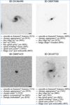 |
Fig. 6 Four examples of the predictions of Zoobot following the structure of the GZH decision tree (see Table 1 and Fig. A.1) for galaxies (inverted greyscale, image ID given above each image) from the complete test set. For every question, the answer with the highest predicted vote fraction (denoted in the parenthesis) is selected. The black bars represent a length of 1″. |
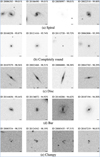 |
Fig. 7 Examples of galaxies with the highest predicted vote fractions of Zoobot for (a) spiral, (b) completely round, (c) disc, (d) barred, and (e) clumpy galaxies from the complete test set. Above each galaxy image, the corresponding image ID and the predicted vote fraction in percent are given. The black bars represent a length of 1″. |
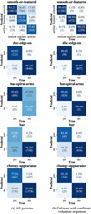 |
Fig. 8 Confusion matrices for five selected morphology questions after binning to the class with the highest predicted vote fraction. The confusion matrices for the other questions are shown in the Appendix. The colour map corresponds to the fraction of the ground truth values for the different classes (also denoted in the confusion matrices). |
 |
Fig. 9 Confusion matrices for the task of finding spiral galaxies in the complete test set by applying the selection cuts suggested in Willett et al. (2017). |
5.2.2 Finding spiral galaxies in the test set
We investigated how Zoobot can be used to find spiral galaxies in a given dataset. Similar to the approach used for volunteer vote fractions f, we applied the suggested criteria from Willett et al. (2017) for selecting spiral galaxies in the complete test set. These criteria were: fedge-on,no > 0.25, fclumpy,no > 0.3, and ffeatures > 0.23. Additionally, we excluded galaxies where the conditions mentioned above apply, but the number of volunteers was insufficient (as Zoobot is only predicting vote fractions), using the suggested cutoff of Nspiral ≥ 20. For the final catalogue, we chose a vote fraction of fspiral > 0.5 to identify spiral galaxies. Thus, all galaxies for which the conditions were fulfilled were classified as spiral, while all the others were classified as not spiral. For the predicted vote fractions, we applied the same cuts. Once more, we measure the performance for confident labels (volunteer vote fraction for the final answer greater than 0.8 or smaller than 0.2).
Zoobot achieves an accuracy of 96.5% for finding spiral galaxies in the complete test set, with an F1-score of 89.6%. The corresponding confusion matrix is shown in Fig. 9a and the corresponding metrics listed in Table 3. On confident labels, Zoobot achieves an accuracy of 97.0% with an F1-score of 89.9% as shown in Fig. 9b and in Table 4. These values demonstrate that Zoobot is indeed well suited for identifying spiral galaxies in a given dataset.
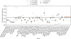 |
Fig. 10 Vote fraction mean deviations δi of the model predictions and the volunteer labels for the different morphology answers i (see Eq. (3)). The model was trained with all galaxies from the complete set. The deviations are displayed for all galaxies of the test set and for galaxies within a magnitude interval with m = mI814W. Lower δi indicates better performance. The black dashed line marks 12% vote fraction mean deviation. |
5.2.3 Vote fraction mean deviations
We then evaluated the model performance by analysing the predicted vote fractions directly. We show the vote fraction mean deviations δi for all answers i corresponding to different morphology types in Fig. 10. Moreover, we display how the performance varies with magnitude by selecting only galaxies from different magnitude intervals.
For almost all answers (36 of 40 answers), the vote fraction mean deviation is below 12%, while the performance varies between different answers. As before, the question with the lowest deviation for all answers is ‘disc-edge-on’. This can be attributed to the fact that it represents a less intricate feature, making it relatively easy to discern and learn. Conversely, questions related to spiral arms and clumps consistently yield the highest deviations. Once again, this can be explained with the inherent complexity of these questions, as they involve finer and more intricate structural details. We expect the quality of the morphological predictions to be better if more relevant labels for these morphology types were available, as indicated in Fig. 5.
The dependence of the vote fraction mean deviation on the magnitude differs between answers. The mean deviation shows no substantial dependence on the magnitude for the ‘smooth-or-features’, ‘disc-edge-on’ and ‘how-rounded’ questions. For the ‘has-spiral-arms’ question, on the other hand, the differences between the deviations are the largest. While the model performs better for brighter galaxies (m < 20.5) with a mean deviation below 10%, for faint galaxies (m > 22) the deviations are the largest overall (~27%). This indicates that identifying spiral arms in faint galaxies is a relatively difficult task. This is not surprising, as spiral arms are a finer structure. Once spiral arms are identified, the other tasks related to spiral arms, such as determining the winding of the spiral arms and counting them, do not show such a strong magnitude dependence. Finally, although clumps appear more frequently for faint galaxies, the model performs better in the case of brighter galaxies. This is not in contradiction to Sect. 5.1.2, where the influence of a magnitude restriction for the galaxies used for training on the model performance on all galaxies of the complete test set was measured. Here, the performance of only one model, trained on all galaxies of the complete training set, is analysed for galaxies of different magnitudes from the complete test set.
5.2.4 Histograms of the vote fraction deviations
While we already investigated the mean of the (absolute) vote fraction deviations fpred – fgt, we show the corresponding histograms for five selected questions in Fig. 11. Positive values indicate that Zoobot predicts a higher vote fraction than the volunteers, and negative values indicate that the volunteer vote fraction is higher.
For most answers, the distributions are centred at 0, indicating that for most galaxies the vote fraction deviations are relatively small. The distributions are symmetrical around the centre, indicating that the model does not have a substantial bias. The widths of the distributions correspond to the mean vote fraction deviations (see Fig. 10), as expected.
In contrast, for the ‘has-spiral-arms’ answers, the distributions are not symmetrical. While the maximum of the distribution is at 0, indicating that most deviations are small, the volunteers’ vote fractions for a galaxy to be spiral are higher than predicted from Zoobot. This can be explained by the high imbalance of the relevant ‘has-spiral-arms’ answers (see Sect. 5.2.1) with the extreme mean vote fraction for ‘yes’ of 90.7% in combination with the intrinsic difficulty of this task. Zoobot predicts for the most extreme volunteer vote fractions (close to 0 or 1) less extreme vote fractions (Walmsley et al. 2022a), leading to the asymmetry of the distribution.
The ‘disc-edge-on’ question also has an imbalance that is slightly less extreme (mean vote fraction for ‘no’ is 83.9%). As it is easier to learn, the vote fraction mean deviation is much smaller (~4%) than for ‘has-spiral-arms’ (~11%). Thus, the imbalance does not lead to a substantial asymmetry of the distribution.
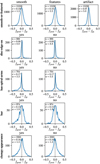 |
Fig. 11 Histograms of the vote fraction deviations fpred – fgt between the predicted fpred and volunteer vote fractions fgt for five selected questions. For each answer, we give the number of galaxies n, the standard deviation σ, and the kurtosis w. |
5.2.5 Magnitude and redshift dependence
Subsequently, we investigated the magnitude and redshift dependence of the mean deviations δi between the predicted and the volunteer vote fractions. These are shown in Figs. 12 and 13 for the different questions. For some galaxies, there was no redshift information available. Thus, these galaxies were excluded.
In general, the vote fraction mean deviation shows no substantial dependence on magnitude and redshift. For relatively easier morphology tasks (for example ‘disc-edge-on’ and ‘smooth-or-featured’) the deviations are smaller than for more complex ones, such as tasks related to spiral arms, bars, and clumps.
For the ‘has-spiral-arms’ question, the vote fraction mean deviation shows a strong increase for z > 1 up to almost 50%. The same effect can be observed for fainter galaxies (mI814W > 21.5 in Fig. 13), although the deviation is smaller. This indicates again that the difficulty of identifying spiral arms for high redshift and faint galaxies is substantially higher than other morphology tasks.
In Fig. 14, we show the volunteer and model vote fraction for the ‘yes’ answer of the ‘has-spiral-arms’ question in a histogram for high-redshift and faint galaxies. For the majority of the galaxies, the volunteer vote fraction is above 90%, meaning that the volunteers are confidently classifying most galaxies to be spiral. Zoobot, on the other hand, shows a wider range of predicted vote fractions, with most being above 70%. While there are no galaxies (for high redshifts) or only one (for faint galaxies) galaxy to be confidently classified to have no spiral arms (vote fraction below 20%), Zoobot is confidently predicting that only two galaxies have no spiral arms. Therefore, Zoobot is not misclassifying galaxies, it is just not as confident as the volunteers. This could be explained with the lower resolution and the additional noise for the emulated Euclid images compared to the original HST images.
To check this, we show the redshift and magnitude dependence for Zoobot trained on the original HST images in Fig. 15. The vote fraction mean deviations are, although still present, substantially smaller than for Euclid images supporting our interpretation. For a practical use, to identify spiral galaxies in high-redshift and high m ranges, the selection cuts can be lowered when applying Zoobot.
5.2.6 Comparing performance to original HST images
While we already investigated the influence of the lower resolution and the additional noise of the Euclid images for identifying spiral arms, we show in Fig. 16 the performance of the model trained and tested on the emulated Euclid images of the complete dataset and trained and tested on the original HST images for the same galaxies (see Sect. 2). The model trained on HST images was additionally tested on emulated Euclid images.
As expected, the model trained and tested on HST images displays the lowest deviations. The deviations of the same model tested on emulated Euclid images are for many answers substantially larger. This can be explained with the lower resolution (which is approximately two times poorer for Euclid compared to HST) and additional noise of the emulated Euclid images. The difference in the deviations varies with the different answers. For example for the ‘disc-edge-on’ question, the deviations are almost the same, supporting the previous discussion that this feature depends less on the resolution. On the other hand, for more complex features, such as spiral arms or clumps, the model performs substantially better for HST images than for Euclid images. This is in agreement with the previous discussion that spiral arms and clumps are finer features and their detection depends on resolution.
The deviations for emulated Euclid images are substantially reduced when the model is trained directly on emulated Euclid images, as shown in Fig. 16. For many questions, such as ‘smooth-or-features’, ‘disc-edge-on’, or ‘how-rounded’, the vote fraction mean deviation is almost the same. However, for questions related to spiral arms, bars and clumps, the performance of Zoobot trained and tested on HST images is still better than for Zoobot trained and tested on Euclid images. This suggests that even when directly using Euclid images in training, due to the lower resolution and noise of the Euclid images, Zoobot performs worse for these finer features.
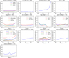 |
Fig. 12 Vote fraction mean deviations δi for all corresponding answers i (different colours denoted in the legend) of the different GZH questions (see Table 1) as a function of redshift z for the relevant galaxies of the complete test set (where at least half of the volunteers voted). |
6 Adapting Zoobot to a new morphology type
We trained Zoobot to emulated Euclid images with the GZH decision tree (see Table 1). Therefore, our model could be directly used for real Euclid images, but is restricted to answering only the questions of the GZH decision tree. However, for Euclid, there might be additional or other galaxy morphology tasks that are currently not included in our Zoobot model. We show that Zoobot can be easily adapted to a new morphology task that is not included in the GZH tasks with the example of peculiar galaxies.
6.1 Adaption procedure
Peculiar galaxies are a type of irregular galaxy, with disorganised structure, often at high redshifts that do not typically fall into smooth, spheroid, or disc classes. The class of peculiar galaxies was not included in the GZH questions. Instead, we used labels for the same emulated Euclid VIS images (see Sect. 2) from a different source, namely expert classification from the Euclid Zoo project1. Euclid Zoo was an internal classification project in the Euclid Consortium, with astronomers as classifiers. In total, 2006 galaxies were classified with N = 1 to N = 3 expert classifications per galaxy image. We selected a galaxy from the dataset to be classified as peculiar if the vote fraction for the peculiar class is larger than 50%, resulting in 231 galaxy images for the peculiar class. In Fig. 17, we show examples of galaxy images and their corresponding labels. We then applied a 70/10/20 percent train/validation/test split, leading to 1404 images for training, 200 for validation and 402 for testing. Next, we balanced our train and validation set by randomly dropping galaxy images that are not peculiar, leading to the same number of ‘not peculiar’ and ‘peculiar’ galaxy images. In total, 308 galaxy images were used for training and 54 for validation.
Similar to Walmsley et al. (2022b), we used our best-performing model (trained on all images from the complete set) and replaced the final output layer by a new model ‘head’, simply consisting of a final dense layer with a sigmoid activation function. We used the Adam optimizer (Kingma & Ba 2015). We then trained the new model with the dataset of peculiar galaxies while applying the same augmentation as before, namely random flips and rotations. To avoid overfitting, we stopped training as soon as the validation loss was not decreasing for 20 consecutive epochs. After training, Zoobot calculated predictions for the 402 images of the test set.
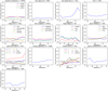 |
Fig. 13 Similar as Fig. 12, but with the vote fraction mean deviations δi depending on the magnitude m. |
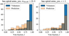 |
Fig. 14 Histograms of the predicted and volunteer vote fractions for the ‘has-spiral-arms’ ‘yes’ answer for faint and high-redshift galaxies. |
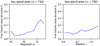 |
Fig. 15 Redshift and magnitude dependence of the ‘has-spiral-arms’ vote fraction mean deviations δi for the model trained on the original HST COSMOS images. Compared to the Euclid images (Figs. 12 and 13), the deviations for high-redshift and faint galaxies are substantially smaller. |
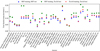 |
Fig. 16 Vote fraction mean deviations of the model predictions and the volunteer labels for the different answers of the decision tree for the model trained and tested on emulated Euclid images and for the model trained on original HST images and tested on emulated Euclid images and on HST images. In all cases, the models were trained and tested with the same galaxies from the complete set. |
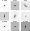 |
Fig. 17 Examples of galaxies and their expert labels as a peculiar or normal galaxy. The black bars represent a length of 1″. There are no distinct morphological features that characterise peculiar galaxies, making this classification task rather difficult. |
Classification metrics accuracy A, precision P, recall R, and the unweighted and weighted F1-scores F1 and ![Mathematical equation: $\[F_1^{\star}\]$](/articles/aa/full_html/2024/09/aa49609-24/aa49609-24-eq20.png) for identifying peculiar galaxies in the test set with different confidence thresholds cth.
for identifying peculiar galaxies in the test set with different confidence thresholds cth.
6.2 Performance of the adapted Zoobot
The performance of the model is listed in Table 5 when evaluated with the classification metrics introduced in Sect. 5.2.1. The corresponding confusion matrices are displayed in Fig. 18. The model achieves an accuracy of 79.1% for a model confidence threshold of cth = 0.5 for selecting a galaxy to be peculiar. By applying cth = 0.75 for our model predictions, we obtain a higher accuracy of 91.5% and a higher F1-score of 81.2% due to significantly higher precision. The values indicate that Zoobot performs well at the task of finding peculiar galaxies.
The accurate identification of peculiar galaxies is particularly impressive, considering that it is a relatively challenging task even for an expert, due to the lack of clear morphological features. In addition to the inherent difficulty, there were only 231 examples of peculiar galaxies, of which 20% were not included in the training dataset. This underscores our earlier discussion regarding the effectiveness of fine-tuning. Our Zoobot model was initially trained on all major GZ campaigns (as described in Sect. 3) and subsequently on GZH using emulated Euclid images, making it well-suited for adaptation to a new Euclid morphology task.
This shows that Zoobot can easily be adapted to new problems, even if these are difficult and do not have many examples. For the application to Euclid, our trained model can be used as a first step to predict detailed morphology for Euclid with the GZH questions and can then be adapted to a new task in an effective way without requiring large labelled sets of galaxy images. Thus, in practice, if an astronomer is interested in finding all examples of a particular galaxy morphological type that is not included in the GZH questions for a given set of real Euclid images, the following steps can be applied. First, a dataset needs to be labelled that is then used to fine-tune the trained Zoobot model to the new galaxy morphology task. Once the model is fine-tuned, it can be used to classify all images of a given set of Euclid images.
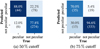 |
Fig. 18 Confusion matrices for finding peculiar galaxies for Zoobot pretrained on the emulated Euclid images and the GZH tasks at (a) 50% and (b) 75% cutoff thresholds cth for selecting peculiar galaxies. |
7 Summary and conclusions
This paper introduces automated and detailed predictions of galaxy morphology for emulated Euclid images. These emulated images were generated by converting HST COSMOS images to Euclid VIS images, considering the Euclid PSF and adjusting them to match the expected noise level of Euclid. The automated predictions were created using Zoobot, a Python package for creating deep learning models that classify galaxy morphology and for adapting (‘fine-tuning’) those models to new surveys and tasks. We fine-tuned a pre-existing Zoobot model (trained on 450 000 non-Euclid galaxies from Galaxy Zoo) using emulated Euclid images and labels derived from the Galaxy Zoo: Hubble (GZH) volunteer responses.
The model is able to accurately predict the detailed morphologies for emulated Euclid galaxy images. It predicts various aspects, including the presence and quantity of clumps, detection, and counting of spiral arms, measurement of their winding, identification of disc galaxies, detection of bars, and determination of the presence, shape, and size of the central bulge, as well as measurement of the shape of featureless galaxies (refer to Table 1).
The Zoobot model fine-tuned on 60 000 available emulated Euclid images with GZH labels achieves a mean deviation of the predicted vote fraction from the volunteer classifications averaged over all answers of 9.5% and below 12% for nearly all answers individually (36 out of 40, as depicted in Fig. 10). Additionally, it achieves an accuracy of above 91% for 12 of 13 questions when considering confident volunteer responses (refer to Table 4). However, the model’s performance varies across different morphology classes.
For the top questions of the decision tree (global morphology type – ‘smooth-or-features’, disc orientation – ‘disc-edge-on’ or ‘bulge-size’), the model is able to predict within 10% of the volunteers’ vote fraction after being trained with only 1000 randomly selected galaxies. For other questions, such as ‘how-rounded’, ‘spiral-arm-count’, or ‘bulge-shape’, 10000 training galaxies are needed, while for questions related to the more complex morphologies, such as ‘has-spiral-arms’, ‘bar’, ‘spiral-winding’, or ‘clumpy-appearance’, the full training set of 60000 galaxies is required to reach 12% deviation from the volunteer classifications. This suggests that using a greater number of examples of complex morphology classes improves the performance of the model. Finally, our investigations of the effects of using the complete sample of available galaxies for training (mI814w < 23.5), or a subset of the brightest galaxies (mI814w < 22.5), suggest that the difference in performance is minimal; the number of galaxies with complex morphologies used for training has a higher impact.
Our results have the following implications for Euclid:
Zoobot, trained on emulated Euclid galaxies using volunteer labels from GZH, shows accurate predictions (within 10% of human classifications) for global morphology (smooth versus featured), disc orientation (edge-on versus face-on), and bulge size.
To enhance the model’s performance in predicting more complex detailed morphologies, such as bars, spiral arms, and clumps, additional labels are required. Based on Fig. 5, approximately 60 000 randomly selected galaxies would be needed to achieve a global vote fraction deviation of below 10% and maintain deviations below 12% for all labels. These additional labels could be obtained by initiating a Galaxy Zoo project for Euclid using Euclid Q1 data.
Our experiments indicate minimal performance differences when selecting galaxies with mI814W < 23.5 or brighter galaxies with mI814W < 22.5. Therefore, we suggest that the pool of explored galaxies for Euclid be expanded with a restriction of IE < 23.5 (assuming VIS magnitudes are reasonably similar to I814W magnitudes). Fainter galaxies were not tested as no morphological labels were available for these galaxies. We expect the fraction of galaxies with features to decrease at higher magnitudes and smaller sizes, as observational effects cause these galaxies to appear smoother.
Zoobot can be adapted to new Euclid morphology tasks using a few new labels. We demonstrate this adaptability by successfully training Zoobot for a new class of peculiar galaxies, consisting of only 261 examples, achieving an accuracy of 91.5% (Fig. 18). Consequently, for new classes, it is feasible to set up a dedicated Galaxy Zoo-style workflow where volunteers are asked simple binary questions related to the morphology of the specific class of interest. The exact number of required labelled galaxies depends on the specific morphology class (Fig. 5).
The proposed morphology classification scheme for Euclid is outlined in a companion paper (Euclid Collaboration: OU-MER, in prep.).
Currently, the generation of structural parameters describing galaxy morphology with a morphology fitting code is included in the Euclid data pipeline (Euclid Collaboration 2023). The algorithm generates morphological parameters for single- and double-Sérsic components, and the measurements are reliable up to Ie = 23 for one component and IE < 21 for two components. Euclid Collaboration (2023) conclude that robust structural parameters will be delivered for at least 400 million galaxies by the Euclid Data Releases.
We estimated the number of galaxies for which detailed morphologies could be measured with our deep learning model. With mI814W < 23.5, there are approximately 70 000 galaxies in an area of (1.2 × 1.2) deg2 = 1.44 deg2 of the HST COSMOS survey. Scaling up to the total sky area measured by the Euclid Wide Survey, of namely 15000 deg2, and assuming that VIS magnitudes are similar to the I814W magnitudes of HST, there would be approximately 800 million galaxies with reliably measured morphologies up to IE = 23.5 (focusing on the brighter magnitudes, IE < 22.5, the estimated count would be approximately 300 million galaxies). This is close to the 400 million galaxies estimated by Euclid Collaboration (2023) for IE < 23. Accounting for an average vote fraction of 29% for galaxies to display features, we conclude that, of the 800 million measured galaxies from the Euclid Wide Survey, approximately 230 million galaxies will display complex morphology. This closely matches the 250 million galaxies that are estimated to have complex structures by Euclid Collaboration (2022a) for the Euclid Wide Survey and the Euclid Deep Survey.
In conclusion, we successfully showcase the feasibility of generating high-quality and detailed morphology predictions for Euclid images. Our trained Zoobot model is now ready for deployment in the Euclid pipeline to produce morphological catalogues for Euclid images with Q1 data. As additional labels for more complex morphologies are obtained, the performance of Zoobot will improve for the upcoming Data Release 1 (DR1). Moreover, the model can be easily adapted to new morphology classes that are of interest to astronomers as new labels are gathered through crowd-sourcing projects.
Acknowledgements
The Euclid Consortium acknowledges the European Space Agency and a number of agencies and institutes that have supported the development of Euclid, in particular the Agenzia Spaziale Italiana, the Belgian Science Policy, the Canadian Euclid Consortium, the French Centre National d’Etudes Spatiales, the Deutsches Zentrum für Luft- und Raumfahrt, the Danish Space Research Institute, the Fundação para a Ciência e a Tecnologia, the Hungarian Academy of Sciences, the Ministerio de Ciencia, Innovación y Universidades, the National Aeronautics and Space Administration, the National Astronomical Observatory of Japan, the Netherlandse Onderzoekschool Voor Astronomie, the Norwegian Space Agency, the Research Council of Finland, the Romanian Space Agency, the State Secretariat for Education, Research and Innovation (SERI) at the Swiss Space Office (SSO), and the United Kingdom Space Agency. A complete and detailed list is available on the Euclid web site (http://www.euclid-ec.org). The data in this paper are the result of the efforts of the Galaxy Zoo volunteers, without whom none of this work would be possible. Their efforts are individually acknowledged at http://authors.galaxyzoo.org. This publication uses data generated via the Zooniverse.org platform, development of which is funded by generous support, including a Global Impact Award from Google, and by a grant from the Alfred P. Sloan Foundation.
Appendix A The GZH decision tree
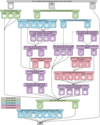 |
Fig. A.1 The original GZH decision tree (Willett et al. 2017). The questions T06, T08, T13, T14 and T15 were not included in this study (see Sect. 4). |
Appendix B Experimenting with different initial weights
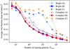 |
Fig. B.1 The vote fraction mean deviation averaged over all answers depending on the number of galaxies used for training for initial weights A (pretraining on GZD-5), B (pretraining on all major GZ campaigns except GZH) and C (no pretraining) and training on the bright and complete training set. In all cases, the predictions were done on the complete test set. Lower values indicate better performance. |
We also conducted the experiment described in the main paper with different initial weights, meaning the utilization of Zoobot pretrained on different data. The weights described in the main text are denoted as weights B. Additionally, we tested with Zoobot pretrained on only GZD-5 (Walmsley et al. 2022a, weights A) and Zoobot without pretraining (random weights, weights C). We show the dependence of the averaged vote fraction mean deviation ![Mathematical equation: $\[\bar{\delta}\]$](/articles/aa/full_html/2024/09/aa49609-24/aa49609-24-eq22.png) on the number of galaxies Ntrain in Fig. B.1. To compare the models, we use in all cases the predictions on the same complete test set of 15 236 images (see Table 2). Additionally, we show for all answers the deviations for all models trained on 100, 1000 and 10 000 galaxies in Figs. B.2, B.3 and B.4.
on the number of galaxies Ntrain in Fig. B.1. To compare the models, we use in all cases the predictions on the same complete test set of 15 236 images (see Table 2). Additionally, we show for all answers the deviations for all models trained on 100, 1000 and 10 000 galaxies in Figs. B.2, B.3 and B.4.
With increasing number of training galaxies, the average mean deviation ![Mathematical equation: $\[\bar{\delta}\]$](/articles/aa/full_html/2024/09/aa49609-24/aa49609-24-eq23.png) is decreasing: The more galaxy examples (of different types) are used for training, the better the model predictions get for all answers. In the regime with Ntrain < 20, the models perform similarly. With more training galaxies, the performance of the model is for all numbers of training galaxies best with initial weights B, followed by weights A and then weights C. The model pretrained on all Galaxy Zoo campaigns except GZH leads, for the same number of galaxies, to a better performance than for a pretraining with only GZD labels. This is due to the better generalization of the model in the pretraining. The model without pretraining (weights C) shows the worst performance of the three, as expected.
is decreasing: The more galaxy examples (of different types) are used for training, the better the model predictions get for all answers. In the regime with Ntrain < 20, the models perform similarly. With more training galaxies, the performance of the model is for all numbers of training galaxies best with initial weights B, followed by weights A and then weights C. The model pretrained on all Galaxy Zoo campaigns except GZH leads, for the same number of galaxies, to a better performance than for a pretraining with only GZD labels. This is due to the better generalization of the model in the pretraining. The model without pretraining (weights C) shows the worst performance of the three, as expected.
Especially, for 100 to 10 000 galaxies, the difference between pretrained models and models used from scratch is most evident. Thus, for a limited number of labelled galaxies, transfer learning is substantially more effective for training to a new problem than training from scratch. In comparison to weights A and B, for weights C, there is a difference between training with bright and with random (complete) galaxies, namely bright galaxies lead to a better model performance especially between 100 and 10 000 galaxies. This difference could be explained with the pretraining for the models with weights A and B. While these have seen many types of galaxies with different magnitudes, they are more reliable and the magnitude cut does not have a significant impact. For weights C, the model was not trained before and thus, learns the galaxies morphologies for the first time. Bright galaxies with morphology that is easier accessible in general seem to be more effective when training from scratch.
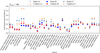 |
Fig. B.2 Vote fraction mean deviations of the model predictions and the volunteer labels for the different answers of the decision tree for the models trained on 100 galaxies of the different datasets (bright and complete) and with different initial weights (weights A, B and C). Lower δi indicates better performance. |
More details of the differences between models are shown in Figs. B.2, B.3 and B.4. The impact of pretraining can be best seen for the ‘disc-edge-on’ question. For the pretrained models (weights A and B), 100 galaxy images are enough in training to get below a deviation of 10%. This deviation is reached for the model from scratch (weights C) at 10000 galaxies. In contrast, for the questions related to clumps, the differences between the models for 100, 1000, and 10000 training galaxies are relatively similar, indicating that the influence of pretraining is smaller for these questions. Only for weights B questions regarding clumps were included in the pretraining, supporting this interpretation.
Appendix C Additional confusion matrices
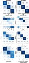 |
Fig. C.1 Confusion matrices continued from Fig. 8 after binning to the class with the highest predicted vote fraction. The colour map corresponds to the fraction of the ground truth values for the different classes. To improve the readability, for the tasks with more than three answers, only the percentage is stated. |
Appendix D Volunteer uncertainty
We show in Fig. D.1 the mean vote fraction deviation δi for the ‘features’ answer of the ‘smooth-or-features’ question, depending on the volunteer vote fraction fgt. In general, the deviations are smaller for confident volunteer responses (vote fraction lower than 0.2 or greater than 0.8) compared to more uncertain volunteer responses (vote fraction between 0.2 and 0.8). As expected, the model performs better for confident volunteer responses and with increasing uncertainty in the volunteer responses the deviations also increase. Moreover, an asymmetry of the deviations can be observed, as deviations are substantially smaller for vote fractions below 0.2 compared to vote fractions above 0.8. This could be explained with the fact that most galaxies of the dataset do not display features. Additionally, the deviations for the lowest volunteer vote fractions are higher than for vote fractions of ~ 0.1. This is due to the characteristic of Zoobot to predict for the most extreme volunteer vote fractions (close to 0 or 1) less extreme vote fractions (Walmsley et al. 2022a), which should not affect practical use.
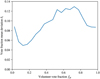 |
Fig. D.1 Vote fraction mean deviations δi of the model predictions and the volunteer labels for the ‘smooth-or-features_features’ answer depending on the volunteer vote fraction fgt. |
Appendix E Reproducibility
The Zoobot CNN is publicly available2. The code for the creation of the images, the training of the Zoobot CNN and for the analysis of the results is also publicly available3.
References
- Abadi, M., Barham, P., Chen, J., et al. 2016, in Proceedings of the 12th USENIX Symposium on Operating Systems Design and Implementation, OSDI’16 [Google Scholar]
- Baillard, A., Bertin, E., de Lapparent, V., et al. 2011, A&A, 532, A74 [NASA ADS] [CrossRef] [EDP Sciences] [Google Scholar]
- Bait, O., Barway, S., & Wadadekar, Y. 2017, MNRAS, 471, 2687 [NASA ADS] [CrossRef] [Google Scholar]
- Cheng, T.-Y., Conselice, C. J., Aragón-Salamanca, A., et al. 2020, MNRAS, 493, 4209 [Google Scholar]
- Conselice, C. J. 2003, ApJS, 147, 1 [NASA ADS] [CrossRef] [Google Scholar]
- Cropper, M., Pottinger, S., Niemi, S., et al. 2016, Proc. SPIE, 9904, 99040Q [Google Scholar]
- de Vaucouleurs, G. 1959, Handbuch Physik, 53, 275 [NASA ADS] [Google Scholar]
- de Vaucouleurs, G., de Vaucouleurs, A., Corwin, Jr., H. G., et al. 1991, Third Reference Catalogue of Bright Galaxies (New York: Springer) [Google Scholar]
- Dey, A., Schlegel, D. J., Lang, D., et al. 2019, AJ, 157, 168 [Google Scholar]
- Dieleman, S., Willett, K. W., & Dambre, J. 2015, MNRAS, 450, 1441 [NASA ADS] [CrossRef] [Google Scholar]
- Domínguez Sánchez, H., Huertas-Company, M., Bernardi, M., Tuccillo, D., & Fischer, J. L. 2018, MNRAS, 476, 3661 [Google Scholar]
- Domínguez Sánchez, H., Huertas-Company, M., Bernardi, M., et al. 2019, MNRAS, 484, 93 [Google Scholar]
- Euclid Collaboration (Bretonnière, H., et al.) 2022a, A&A, 657, A90 [CrossRef] [EDP Sciences] [Google Scholar]
- Euclid Collaboration (Scaramella, R., et al.) 2022b, A&A, 662, A112 [NASA ADS] [CrossRef] [EDP Sciences] [Google Scholar]
- Euclid Collaboration (Bretonnière, H., et al.) 2023, A&A, 671, A102 [NASA ADS] [CrossRef] [EDP Sciences] [Google Scholar]
- Griffith, R. L., Cooper, M. C., Newman, J. A., et al. 2012, ApJS, 200, 9 [NASA ADS] [CrossRef] [Google Scholar]
- Grogin, N. A., Kocevski, D. D., Faber, S. M., et al. 2011, ApJS, 197, 35 [NASA ADS] [CrossRef] [Google Scholar]
- Hubble, E. P. 1926, ApJ, 64, 321 [Google Scholar]
- Huertas-Company, M., Gravet, R., Cabrera-Vives, G., et al. 2015, ApJS, 221, 8 [NASA ADS] [CrossRef] [Google Scholar]
- Ivezić, Ž., Kahn, S. M., Tyson, J. A., et al. 2019, ApJ, 873, 111 [Google Scholar]
- Kaifu, N., Usuda, T., Hayashi, S. S., et al. 2000, PASJ, 52, 1 [NASA ADS] [Google Scholar]
- Kingma, D. P., & Ba, J. 2015, in 3rd International Conference on Learning Representations, ICLR 2015 – Conference Track Proceedings [Google Scholar]
- Koekemoer, A. M., Aussel, H., Calzetti, D., et al. 2007, ApJS, 172, 196 [Google Scholar]
- Kruk, S. J., Lintott, C. J., Bamford, S. P., et al. 2018, MNRAS, 473, 4731 [Google Scholar]
- Laureijs, R., Amiaux, J., Arduini, S., et al. 2011 arXiv e-prints [arXiv:1110.3193] [Google Scholar]
- Lintott, C. J., Schawinski, K., Slosar, A., et al. 2008, MNRAS, 389, 1179 [NASA ADS] [CrossRef] [Google Scholar]
- Lotz, J. M., Primack, J., & Madau, P. 2004, AJ, 128, 163 [NASA ADS] [CrossRef] [Google Scholar]
- Lu, J., Behbood, V., Hao, P., et al. 2015, Knowledge-Based Syst., 80, 14 [Google Scholar]
- Masters, K. L. 2019, Proc. Int. Astron. Union, 14, 205 [CrossRef] [Google Scholar]
- Masters, K. L., Mosleh, M., Romer, A. K., et al. 2010, MNRAS, 405, 783 [NASA ADS] [Google Scholar]
- Peng, C. Y., Ho, L. C., Impey, C. D., & Rix, H.-W. 2002, AJ, 124, 266 [Google Scholar]
- Sakamoto, K., Okumura, S. K., Ishizuki, S., & Scoville, N. Z. 1999, ApJ, 525, 691 [NASA ADS] [CrossRef] [Google Scholar]
- Sandage, A. 1961, The Hubble Atlas of Galaxies (Washington: Carnegie Institution) [Google Scholar]
- Scoville, N., Abraham, R. G., Aussel, H., et al. 2007a, ApJS, 172, 38 [NASA ADS] [CrossRef] [Google Scholar]
- Scoville, N., Aussel, H., Brusa, M., et al. 2007b, ApJS, 172, 1 [Google Scholar]
- Sérsic, J. L. 1968, Atlas de galaxias australes (Cordoba, Argentina: Observatorio Astronomico) [Google Scholar]
- Simmons, B. D., Lintott, C., Willett, K. W., et al. 2017, MNRAS, 464, 4420 [Google Scholar]
- Tan, M., & Le, Q. V. 2019, arXiv e-prints [arXiv:1905.11946] [Google Scholar]
- Taniguchi, Y., Scoville, N., Murayama, T., et al. 2007, ApJS, 172, 9 [Google Scholar]
- van den Bergh, S. 1976, ApJ, 206, 883 [NASA ADS] [CrossRef] [Google Scholar]
- Vega-Ferrero, J., Domínguez Sánchez, H., Bernardi, M., et al. 2021, MNRAS, 506, 1927 [NASA ADS] [CrossRef] [Google Scholar]
- Walmsley, M., Lintott, C., Géron, T., et al. 2022a, MNRAS, 509, 3966 [Google Scholar]
- Walmsley, M., Scaife, A. M. M., Lintott, C., et al. 2022b, MNRAS, 513, 1581 [NASA ADS] [CrossRef] [Google Scholar]
- Walmsley, M., Slijepcevic, I. V., Bowles, M., & Scaife, A. M. M. 2022c, Machine Learning for Astrophysics Workshop at the 39th International Conference on Machine Learning, (ICML 2022), online at https://ml4astro.github.io/icml2022, 29 [Google Scholar]
- Walmsley, M., Allen, C., Aussel, B., et al. 2023a, J. Open Source Softw., 8, 5312 [NASA ADS] [CrossRef] [Google Scholar]
- Walmsley, M., Géron, T., Kruk, S., et al. 2023b, MNRAS, 526, 4768 [Google Scholar]
- Willett, K. W., Lintott, C. J., Bamford, S. P., et al. 2013, MNRAS, 435, 2835 [Google Scholar]
- Willett, K. W., Galloway, M. A., Bamford, S. P., et al. 2017, MNRAS, 464, 4176 [NASA ADS] [CrossRef] [Google Scholar]
All Tables
Classification metrics accuracy A, precision P, recall R, and the unweighted and weighted F1-scores F1 and for identifying peculiar galaxies in the test set with different confidence thresholds cth.
All Figures
|
Fig. 1 Data pipeline scheme for the emulated Euclid VIS images created as part of the Euclid Data Challenge 2. The green numbers correspond to the numbers of the description of the pipeline given in the text. |
| In the text | |
|
Fig. 2 Examples of galaxy images (inverted greyscale) of different morphological types (image IDs 20092952, 20172737, 20177553, 20107313): (a) from the original HST COSMOS dataset, (b) from the emulated Euclid VIS dataset, and (c) from the Subaru dataset. The images are scaled with galaxy size using three times the Kron radius. The black bars represent a length of 1″. The image IDs are the unique identifiers for the galaxies of the COSMOS survey (Griffith et al. 2012). |
| In the text | |
|
Fig. 3 Vote fraction mean deviation averaged over all morphology answers |
| In the text | |
|
Fig. 4 Vote fraction mean deviations δi of the model predictions and the volunteer labels for the different morphology answers i (see Eq. (3)), for models trained on 1000 bright or random galaxies from the complete set. Lower δi indicates better performance. |
| In the text | |
|
Fig. 5 Vote fraction mean deviations of the model predictions |
| In the text | |
|
Fig. 6 Four examples of the predictions of Zoobot following the structure of the GZH decision tree (see Table 1 and Fig. A.1) for galaxies (inverted greyscale, image ID given above each image) from the complete test set. For every question, the answer with the highest predicted vote fraction (denoted in the parenthesis) is selected. The black bars represent a length of 1″. |
| In the text | |
|
Fig. 7 Examples of galaxies with the highest predicted vote fractions of Zoobot for (a) spiral, (b) completely round, (c) disc, (d) barred, and (e) clumpy galaxies from the complete test set. Above each galaxy image, the corresponding image ID and the predicted vote fraction in percent are given. The black bars represent a length of 1″. |
| In the text | |
|
Fig. 8 Confusion matrices for five selected morphology questions after binning to the class with the highest predicted vote fraction. The confusion matrices for the other questions are shown in the Appendix. The colour map corresponds to the fraction of the ground truth values for the different classes (also denoted in the confusion matrices). |
| In the text | |
|
Fig. 9 Confusion matrices for the task of finding spiral galaxies in the complete test set by applying the selection cuts suggested in Willett et al. (2017). |
| In the text | |
|
Fig. 10 Vote fraction mean deviations δi of the model predictions and the volunteer labels for the different morphology answers i (see Eq. (3)). The model was trained with all galaxies from the complete set. The deviations are displayed for all galaxies of the test set and for galaxies within a magnitude interval with m = mI814W. Lower δi indicates better performance. The black dashed line marks 12% vote fraction mean deviation. |
| In the text | |
|
Fig. 11 Histograms of the vote fraction deviations fpred – fgt between the predicted fpred and volunteer vote fractions fgt for five selected questions. For each answer, we give the number of galaxies n, the standard deviation σ, and the kurtosis w. |
| In the text | |
|
Fig. 12 Vote fraction mean deviations δi for all corresponding answers i (different colours denoted in the legend) of the different GZH questions (see Table 1) as a function of redshift z for the relevant galaxies of the complete test set (where at least half of the volunteers voted). |
| In the text | |
|
Fig. 13 Similar as Fig. 12, but with the vote fraction mean deviations δi depending on the magnitude m. |
| In the text | |
|
Fig. 14 Histograms of the predicted and volunteer vote fractions for the ‘has-spiral-arms’ ‘yes’ answer for faint and high-redshift galaxies. |
| In the text | |
|
Fig. 15 Redshift and magnitude dependence of the ‘has-spiral-arms’ vote fraction mean deviations δi for the model trained on the original HST COSMOS images. Compared to the Euclid images (Figs. 12 and 13), the deviations for high-redshift and faint galaxies are substantially smaller. |
| In the text | |
|
Fig. 16 Vote fraction mean deviations of the model predictions and the volunteer labels for the different answers of the decision tree for the model trained and tested on emulated Euclid images and for the model trained on original HST images and tested on emulated Euclid images and on HST images. In all cases, the models were trained and tested with the same galaxies from the complete set. |
| In the text | |
|
Fig. 17 Examples of galaxies and their expert labels as a peculiar or normal galaxy. The black bars represent a length of 1″. There are no distinct morphological features that characterise peculiar galaxies, making this classification task rather difficult. |
| In the text | |
|
Fig. 18 Confusion matrices for finding peculiar galaxies for Zoobot pretrained on the emulated Euclid images and the GZH tasks at (a) 50% and (b) 75% cutoff thresholds cth for selecting peculiar galaxies. |
| In the text | |
|
Fig. A.1 The original GZH decision tree (Willett et al. 2017). The questions T06, T08, T13, T14 and T15 were not included in this study (see Sect. 4). |
| In the text | |
|
Fig. B.1 The vote fraction mean deviation averaged over all answers depending on the number of galaxies used for training for initial weights A (pretraining on GZD-5), B (pretraining on all major GZ campaigns except GZH) and C (no pretraining) and training on the bright and complete training set. In all cases, the predictions were done on the complete test set. Lower values indicate better performance. |
| In the text | |
|
Fig. B.2 Vote fraction mean deviations of the model predictions and the volunteer labels for the different answers of the decision tree for the models trained on 100 galaxies of the different datasets (bright and complete) and with different initial weights (weights A, B and C). Lower δi indicates better performance. |
| In the text | |
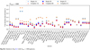 |
Fig. B.3 Similar to Fig. B.2 with Ntrain = 1000 galaxies. |
| In the text | |
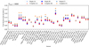 |
Fig. B.4 Similar to Fig. B.2 with Ntrain = 10 000 galaxies. |
| In the text | |
|
Fig. C.1 Confusion matrices continued from Fig. 8 after binning to the class with the highest predicted vote fraction. The colour map corresponds to the fraction of the ground truth values for the different classes. To improve the readability, for the tasks with more than three answers, only the percentage is stated. |
| In the text | |
|
Fig. D.1 Vote fraction mean deviations δi of the model predictions and the volunteer labels for the ‘smooth-or-features_features’ answer depending on the volunteer vote fraction fgt. |
| In the text | |
Current usage metrics show cumulative count of Article Views (full-text article views including HTML views, PDF and ePub downloads, according to the available data) and Abstracts Views on Vision4Press platform.
Data correspond to usage on the plateform after 2015. The current usage metrics is available 48-96 hours after online publication and is updated daily on week days.
Initial download of the metrics may take a while.