| Issue |
A&A
Volume 687, July 2024
|
|
|---|---|---|
| Article Number | A88 | |
| Number of page(s) | 16 | |
| Section | Astrophysical processes | |
| DOI | https://doi.org/10.1051/0004-6361/202449497 | |
| Published online | 28 June 2024 | |
Impacts of nonthermal emission on the images of a black hole shadow and extended jets in two-temperature GRMHD simulations
1
Tsung-Dao Lee Institute, Shanghai Jiao Tong University, Shanghai 201210, PR China
e-mail: This email address is being protected from spambots. You need JavaScript enabled to view it.
, This email address is being protected from spambots. You need JavaScript enabled to view it.
2
College of Physics, Jilin University, Changchun 130012, PR China
3
School of Physics and Astronomy, Shanghai Jiao Tong University, Shanghai 200240, PR China
4
Institut für Theoretische Physik, Goethe Universität, Max-von-Laue-Str. 1, 60438 Frankfurt, Germany
5
Institut für Theoretische Physik und Astrophysik, Universität Würzburg, Emil-Fischer-Str. 31, 97074 Würzburg, Germany
6
Max-Planck-Institut für Radioastronomie, Auf dem Hügel 69, 53121 Bonn, Germany
7
Mullard Space Science Laboratory, University College London, Holmbury St. Mary, Dorking, Surrey RH5 6NT, UK
8
Instituto de Astronomía, Universidad Nacional Autónoma de México, AP 70-264, Ciudad de México 04510, Mexico
Received:
5
February
2024
Accepted:
3
April
2024
Abstract
Context. The recent 230 GHz observations from the Event Horizon Telescope (EHT) collaboration are able to image the innermost structure of the M87 galaxy showing the shadow of the black hole, a photon ring, and a ring-like structure that agrees with thermal synchrotron emission from the accretion disc. However, at lower frequencies, M87 is characterized by a large-scale jet with clear signatures of nonthermal emission. It is necessary to explore the impacts of nonthermal emission on black hole shadow images and extended jets, especially at lower frequencies.
Aims. In this study, we aim to compare models with different electron heating prescriptions to one another and to investigate how these prescriptions and nonthermal electron distributions may affect black hole shadow images and the broadband spectrum energy distribution (SED) function.
Methods. We performed general relativistic radiative transfer (GRRT) calculations in various two-temperature general relativistic magnetohydrodynamic (GRMHD) models utilizing different black hole spins and different electron heating prescriptions coupled with different electron distribution functions (eDFs).
Results. Through a comparison with GRRT images and SEDs, we found that when considering a variable κ eDF, the parameterized prescription of the R − β electron temperature model with Rh = 1 is similar to the model with electron heating in the morphology of images, and the SEDs at a high frequency. This is consistent with previous studies using the thermal eDF. However, the nuance between them could be differentiated through the diffuse extended structure seen in GRRT images, especially at a lower frequency, and the behavior of SEDs at low frequency. The emission from the nearside jet region is enhanced in the case of electron heating provided by magnetic reconnection and it will increase if the contribution from the regions with stronger magnetization is included or if the magnetic energy contribution to κ eDF mainly in the magnetized regions is considered. Compared with the thermal eDF, the peaks of the SEDs shift to a lower frequency when we consider nonthermal eDF.
Key words: Black hole physics / accretion / accretion disks / magnetic reconnection / radiation mechanisms: non-thermal / radiative transfer
© The Authors 2024
 Open Access article, published by EDP Sciences, under the terms of the Creative Commons Attribution License (https://creativecommons.org/licenses/by/4.0), which permits unrestricted use, distribution, and reproduction in any medium, provided the original work is properly cited.
This article is published in open access under the Subscribe to Open model. This email address is being protected from spambots. You need JavaScript enabled to view it. to support open access publication.
1. Introduction
The supermassive black hole M87 * is an ideal object that can be observed directly, and the study of its black hole shadow is of great scientific significance. The Event Horizon Telescope (EHT) collaboration utilized very-long-baseline interferometer (VLBI) technology to network eight radio telescopes around the world into forming a virtual telescope with an effective diameter equivalent to the diameter of the Earth, which makes the direct observation of supermassive black holes possible. There are two main targets: the black hole at the Galactic center, Sgr A*, and the black hole in the nearby elliptical galaxy M87. M87 is somehow an ideal object for direct observation due to its characteristics of long periods and a lack of interstellar scattering interference (Bower et al. 2006) with the presence of a powerful radio jet (Broderick & Loeb 2009). Theoretically, when one looks at the black hole, one can see the black hole shadow, which is the silhouette of the unstable light region around the event horizon (Cunningham & Bardeen 1973; Damour & Polyakov 1994; Grenzebach et al. 2014; Younsi et al. 2016). The study of black hole shadows provides insights into their mass, inclination angle, and spin, making it one of the most rigorous tests of general relativity.
Numerical modeling helps us understand the physics behind black hole shadows. Observations provide a reference for model prediction, while the synthetic images are made by the general relativistic magnetohydrodynamic (GRMHD) simulation and general relativistic radiative transfer (GRRT) calculations. Comparison between synthetic images and observations shows whether the physical models are correct. At present, numerical modeling has been effective. A ring-like structure as the most direct observational evidence of a black hole shadow is mostly consistent with the synthetic models given by the GRMHD simulations (EHT Collaboration 2019a,b,c,d,e,f).
General relativistic magnetohydrodynamic simulations are helpful in improving our understanding of accretion physics. Generally, M87 is believed to have a low accretion rate consisting of a geometrically thick but optically thin accretion disk in a state of radiatively inefficient accretion flow (RIAF; Narayan & Yi 1995; Yuan & Narayan 2014). It has been found that the mass accretion rate of M87 is several orders of magnitude smaller than the Eddington limit, and its brightness is much smaller than the corresponding Eddington brightness (Ho 2009). Similarly, Faraday rotation measurements provide indirect evidence for the low accretion rate of M87 (Bower et al. 2003; Marrone et al. 2007; Kuo et al. 2014). In order to study the radiative signature at the event horizon scale in M87, many GRMHD simulations have been performed in the RIAF state around the rotating black hole (Komissarov 1999; De Villiers & Hawley 2003; Noble et al. 2007; Mościbrodzka et al. 2009, 2014, 2016; Dexter et al. 2010; Shcherbakov et al. 2012; Davelaar et al. 2018, 2019; Olivares Sánchez et al. 2018; Mizuno et al. 2018).
General relativistic radiative transfer calculations utilize GRMHD simulation data to compute black hole shadow images, light curves, and spectrum energy distributions (SEDs). GRMHD codes typically focus only on ions that are important for fluid evolution and provide little information about electrons. Therefore, the calculation of important parameters for modeling the electromagnetic radiation of accreting black holes, such as the electron distribution function (eDF) and electron temperature, becomes an open problem (Davelaar et al. 2019). In terms of the eDF, in the GRMHD simulation of M87, the EHT collaboration assumed that the eDF of all simulation regions is the Maxwell-Jüttner distribution (EHT Collaboration 2019e). However, the energy distribution of electrons depends on energy dissipation, particle acceleration, and thermalization (Yuan & Narayan 2014). If only the thermal distribution is considered, some potentially important nonthermal effects will be ignored, such as magnetic reconnection and turbulent dissipation, which will accelerate electrons to the nonthermal power law distribution (Ding et al. 2010; Hoshino 2013). In addition, some features of M87 caused by electron acceleration have been observed in the near-infrared and optical bands (Prieto et al. 2016). Therefore, the impacts of nonthermal distribution merit consideration. In view of the influence of nonthermal distributed electrons on images, a so-called κ distribution (Vasyliunas 1968), which can both reproduce thermal-electron distribution and present power law distribution characteristics at high energies by adjusting parameters, attracts people’s interest. Later, one can use the GRMHD simulations in a standard accretion and normal evolution (SANE) state (Narayan et al. 2012; Sądowski et al. 2013) in GRRT calculations to study the black hole shadow using the κ eDF (Davelaar et al. 2018, 2019). Recently, the application of the κ distribution to magnetically arrested disk (MAD) models (Narayan et al. 2003; Tchekhovskoy et al. 2011) has reproduced the wide opening angle jet morphology at 86 GHz and fit the broadband spectrum of M87 from the radio to the near-infrared bands (Cruz-Osorio et al. 2022). Besides, compared with SANE models, Fromm et al. (2022) indicate that the broad and highly magnetized jet illuminated by the nonthermal electrons stemming from the κ distribution emerges in R − β models with the MAD state. Furthermore, Davelaar et al. (2023) show the propagation of waves along the shear layer of the jet wind using the κ distribution in the MAD regime.
As is shown in VLBI multi-wavelength observations of M87 * (EHT MWL Science Working Group 2021), the spectral index, α, is estimated between −1 ≤ α ≤ 0, which indicates the existence of nonthermal distributions of electrons. Motivated by the indication of the existence of electrons in observation, to self-consistently understand the contribution of the nonthermal emission in the images, it is necessary to investigate the impacts of nonthermal emission on black hole shadow images in two-temperature GRMHD simulations. A previous study using a three-dimensional two-temperature GRMHD simulation with thermal distribution on the MAD state of M87 has been conducted by Mizuno et al. (2021). The results of the elementary parameterized R − β model were found to be consistent with those of complicated electron-heating models at 230 GHz when considering the Maxwell-Jüttner distribution. However, the impacts of nonthermal electrons on shadow images and the features at different frequencies were not investigated in the previous work. Therefore, the nonthermal distribution, or the κ distribution, is left for this paper to study.
This paper is arranged as follows: Section 1 gives a brief overview of the background. In Sect. 2, we introduce two electron heating prescriptions used in GRMHD simulations and the nonthermal eDFs used in the GRRT calculation. The results of the GRRT calculation, light curves, and SEDs are shown in Sect. 3. In Sect. 4, we discuss our results and the limitations of our study.
Throughout this paper, we adopt units where the speed of light is c = 1 and the gravitational constant is G = 1. We absorb a factor of  into the definition of the magnetic field 4-vector, bμ.
2. Numerical setup
In this section, the computational methods are described. This includes the two-temperature GRMHD simulation data and two electron heating prescriptions used in this paper. Subsequently, an account is given of the traditional methods and the new methodology for the eDFs used in the GRRT calculation at the end of this section.
2.1. General relativistic magnetohydrodynamic setup
We used the same GRMHD simulation data in previous studies (Mizuno et al. 2021; Fromm et al. 2022). There are three-dimensional two-temperature GRMHD simulations of magnetized accretion flows using the BHAC code (Porth et al. 2017; Olivares et al. 2019). The metric adopted in the simulation is spherically modified Kerr-Schild (MKS) coordinates. The simulations were performed up to t = 15 000 M. They reach a quasi-stationary MAD state (see Appendix D for more details). The time evolution of electron temperature in two-temperature GRMHD simulations is based on solving the electron entropy equation (Ressler et al. 2015; Mizuno et al. 2021). The detailed initial setup is described in the following papers (Mizuno et al. 2021; Cruz-Osorio et al. 2022; Fromm et al. 2022).
In the GRMHD simulation, electron heating is provided by grid-scale dissipation. Although it is mostly numerical, we consider grid-scale dissipation to mimic physical processes to heat the electrons (Ressler et al. 2015). The physical processes include turbulent heating, magnetic reconnection, shock waves, and Ohmic dissipation. This paper uses two heating models: turbulence (Kawazura et al. 2019) and magnetic reconnection (Rowan et al. 2017).
2.2. General relativistic radiative transfer setup
In order to calculate images of black hole shadows from GRMHD simulations, this paper uses the GRRT code BHOSS (Younsi et al. 2012, 2020, 2023), which solves the equations of covariant radiative transfer via the ray-tracing method. The synchrotron radiation from electrons, as a radiation mechanism, is considered in this paper.
This paper considers two forms of the eDF. One is the Maxwell-Jüttner distribution given by Eq. (1) and the other is the κ distribution, which can simultaneously represent thermal electron distribution properties and power law characteristics by adjusting certain parameters of Eq. (2). The Maxwell-Jüttner distribution is expressed as follows:
 (1)
(1)
where ne is the electron number density, γe is the electron Lorentz factor, K2 is the Bessel function of the second kind, and Θe is the dimensionless electron temperature (see, e.g., Mizuno et al. 2021).
The relativistic nonthermal κ distribution (Xiao 2006) is expressed as follows:
 (2)
(2)
where N is the normalization factor (Pandya et al. 2016; Davelaar et al. 2019) and κ is related to the slope of the power law distribution, s = κ − 1. When γe is large, particles satisfy  and the nonthermal κ distribution approximates the power law distribution. The parameter w specifies the width of a κ distribution. Considering the contribution of both thermal energy and magnetic energy to heating and accelerating electrons (Davelaar et al. 2019; Cruz-Osorio et al. 2022; Fromm et al. 2022), the specific expression of w is written as follows:
![Mathematical equation: $$ \begin{aligned} w:=\frac{\kappa -3}{\kappa } \Theta _{\mathrm{e} }+\frac{\varepsilon }{2}\left[1+\tanh \left(r-r_{\mathrm{inj} }\right)\right] \frac{\kappa -3}{6 \kappa } \frac{m_{\mathrm{p} }}{m_{\mathrm{e} }} \sigma \,, \end{aligned} $$](/articles/aa/full_html/2024/07/aa49497-24/aa49497-24-eq5.gif) (3)
(3)
where rinj is the injection radius, me is the electron mass, mp is the proton mass, σ = b2/ρ is the magnetization, b2 is the square of a 4-magnetic field, ρ is the fluid rest-mass density, and ε is a tunable parameter for the region with a radius larger than rinj. The energy is dominated by thermal energy with a limit of σ ≪ 1, while the magnetic energy contributes to magnetized regions. We consider ε to be zero or nonzero. We set ε = 0 by default to study the impacts of the κ distribution with thermal energy and show the results with a constant ε = 0.5 in Appendix A for the discussion of the magnetic energy contribution to the GRRT images and the spatial distribution of w. The jet stagnation surface is a potential injection site and defines the injection radius. The stagnation surface is located at ur = 0, where the potential injection radius is usually between 5 M and 10 M (Nakamura et al. 2018). We therefore assumed rinj = 10 M in this study.
Two κ values were used throughout: a fixed κ value with κ = 3.5, and a variable value of κ defined to be parametrically dependent on magnetization, σ, and plasma beta, β = pg/pm, where pg is the fluid pressure and pm = b2/2 is the magnetic pressure:
 (4)
(4)
which was obtained empirically from particle-in-cell (PIC) simulations of the Harris current sheet (Ball et al. 2018) (see also Meringolo et al. 2023 for results using PIC simulations of turbulent plasma). The distribution of accelerated ions is well fit by the fixed κ distribution shown in the PIC simulation (Kunz et al. 2016). We also considered a fixed κ distribution for electrons and set κ = 3.5 based on the prediction of the spectral index of α ≈ −0.7 for MAD models regardless of spin (Ricarte et al. 2023), with α = −(κ − 2)/2.
In this study, we used two methods to obtain the electron temperature for the GRRT calculations. The first method estimated the electron temperature from a parametric prescription, here the “R − β” model (Mościbrodzka et al. 2009). The second method directly calculated the electron temperature from the two-temperature GRMHD simulations (Mizuno et al. 2021). The parametric R − β model is given by
 (5)
(5)
where Rl and Rh are hyperparameters, and Ti is the plasma ion temperature and electron temperature, Te = mec2Θe/kB, in c.g.s. units, where kB is Boltzmann’s constant and c is the speed of light. When Rl is fixed, the ratio of ion-to-electron temperatures in the strongly magnetized region (β ≪ 1) is approximately Rl, and thus the temperature of electrons in the highly magnetized jet does not change with Rh. Conversely, in weakly magnetized regions, the ratio of ion-to-electron temperatures is approximately Rh. We note that the image comparison results do not depend on the value of Rl (Mizuno et al. 2021). Therefore, we fixed Rl = 1 and varied Rh as Rh = (1, 10, 80, 160).
For the GRRT calculation, we modeled M87 * with a mass, MBH = 6.5 × 10⁹ M⊙, at a distance, D = 16.8 Mpc (EHT Collaboration 2019f). The field of view (FoV) was initialized to be 320 μas in both directions and the resolution was 640 × 640 pixels. The calculations were performed from t = 14 000 M to t = 15 000 M, with a 10 M cadence. The time-averaged flux was set to be 0.5 Jy at 230 GHz at 163° in the entire current FoV; thus, at any given time the images at 86 GHz or 43 GHz, and at 163° or 60°, share the same mass accretion rate as those calculated at 230 GHz at 163°. The ceiling to exclude regions with strong magnetization was σcut = 1 by default and we varied σcut as σcut = (1, 2, 5, 10) in Sect. 3.6.
3. Results
3.1. General relativistic radiative transfer calculation
Figures 1 and 2 depict time-averaged GRRT images at 230 GHz and 86 GHz using different nonthermal eDFs, spins, and electron heating prescriptions in logarithmic intensity scaling. In general, all cases show a bright photon ring with some diffuse extended structures. We see that the extended structure is more prominent in 86 GHz.
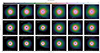 |
Fig. 1. Time-averaged GRRT images of MAD simulations with various black hole spins and eDFs at 230 GHz with an inclination angle of 163°. From top to bottom: black hole spins with a = −0.9375, 0, and 0.9375, respectively. From left to right: the variable κ eDF using the R − β model with Rh = 1, turbulent and reconnection heating, and a fixed κ eDF, with κ = 3.5 using the R − β model with Rh = 1, turbulent and reconnection heating prescriptions. The dashed white contour indicates the curve with 1% of the maximum flux. The time-averaged total flux is 0.5 Jy at 230 GHz, with a simulation time span from t = 14 000 to 15 000 M. |
In the comparison between electron heating and parameterized R − β prescriptions, the results indicate that the morphological structure of the turbulent heating model is matched with the one using the R − β model with Rh = 1 in all spin cases, using the variable κ eDF.
Compared to images of variable κ eDF cases, extended emission is prominently displayed in the images using fixed κ eDF, as was expected. This is because we employed a uniformly large nonthermal electron population, even in regions with low magnetization. It should be noted that the central bright ring is mainly attributed to the region near the black hole, mostly by thermal components (EHT Collaboration 2019e), while the extended diffuse emission comes from the jet sheath or wind region that is profoundly influenced by the choice of eDF. When considering a model with fixed κ = 3.5, compared with thermal or variable κ eDF, the nonthermal power law tail of the eDF is well extended (see Fig. 4 in Fromm et al. 2022). Therefore, in the fixed κ eDF case, the extended diffuse emission becomes more luminous, while the maximum flux becomes slightly lower than that of the variable κ eDF because we set the total flux to be fixed.
Moreover, as is shown in the corotating cases, there is a semi-arc-like structure in the images of the reconnection heating model. The extended semi-arc-like structure represents the enhancement of emission on the nearside jet shown in Fig. 4, in the reconnection heating cases. Such a semi-arc-like extended structure is likely to be the propagation of Alfvén waves or the emerging magnetic flux tube (Moriyama et al. 2024; Jiang et al. 2023).
Conversely, the presence of extended structure not only relies on heating prescriptions but also relates to their spins. The differences between the jet width and the jet length for the different spins can be related to the variability of the accretion flow and the accreted magnetic flux (Fromm et al. 2022). The extended structure in nonrotating cases would be different from the highly rotating cases due to the emission mainly coming from outflowing winds or accretion flows instead of highly magnetized powerful jets due to the lack of an ergosphere (Blandford & Znajek 1977). In counter-rotating cases, the rotation direction between the accretion flow and the black hole is opposed. Consequently, at the same inclination angle, the flow direction is different from the corotating cases, which causes the distinct enhancement of extended jet regions. In counter-rotating cases, the inner stable circular orbit (ISCO) position (RISCO ≈ 8.8 M) is far from the black hole horizon, inducing a dim photon ring and enhancement of the extended structure. The counter-rotating cases exhibit more elongated or elliptical structures, while corotating cases show homogeneous or spherical structures. As is shown in Fig. 2 at 86 GHz, the differences stemming from spins become bigger.
Figure 3 presents the time-averaged corotating GRRT images at 230 GHz with the inclination angle i = 60° on a logarithmic scale in different electron heating prescriptions and eDF models. In comparing the thermal and the κ eDFs, images of fixed κ = 3.5 have a clear diffuse extended structure and this trend is also seen in the images with an inclination angle of 163°. The images of variable κ are analogous to thermal ones except for the small differences in the extended structure and the maximum flux. The images using reconnection heating lead to a smaller vertical extended structure, in contrast with the ones of the turbulent heating or the R − β prescriptions. This difference in vertically extended structure results from the difference in the contribution to the emission from the midplane region (see Appendix B for more details).
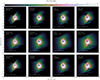 |
Fig. 3. Time-averaged GRRT images of MAD simulations with a black hole spin of a = 0.9375 at 230 GHz and an inclination angle of 60°. From top to bottom: the eDF models using thermal, fixed κ = 3.5, and variable κ, respectively. From left to right: electron heating prescriptions using reconnection heating, turbulent heating, and the R − β model with Rh = 1 and Rh = 160, respectively. The dashed white contour indicates the curve with 1% of the maximum flux. The time-averaged total flux is 0.5 Jy from t = 14 000 to 15 000 M at 163°. |
3.2. Image decomposition
Decomposed images are designed to evaluate what portion of the emission coming from the different regions contributes to the total images. We divided the three regions, the midplane, the nearside jet, and the farside jet, into decomposed images, following the previous study (EHT Collaboration 2019e). Figure 4 displays the changes in the ratio of the emission contributed by decomposed regions at 230 GHz in different heating models with a variable κ eDF. The percentage shown in the bottom right corner indicates the ratio of the emission contributed by a region relative to the total image. From the results, we can confirm that the diffuse extended jet structure seen in all heating models arises mostly from the emission from the nearside jet. The proportion of emission from the nearside jet differs slightly, ranging from 2.4% in the R − β model (Rh = 1) to 3.5% in the reconnection heating model, at 230 GHz. Strikingly, as is shown in Fig. 5, the emission coming from nearside jet accounts for 6.7% of the total emission at 86 GHz and even reaches 14.5% at 43 GHz. It indicates that the contribution from the nearside jet emission increases at lower frequencies.
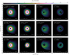 |
Fig. 4. Time-averaged GRRT decomposed images with a black hole spin of a = 0.9375 at 230 GHz with a 163° inclination angle. From top to bottom: images using the R − β model with Rh = 1, the turbulent heating model, and the reconnection heating model, respectively. From left to right, the emissions come from every region: the whole region is depicted first, then the midplane, the nearside jet, and the farside jet, respectively. The eDF of all of the images is variable κ and the time-averaged total flux is 0.5 Jy at 230 GHz from t = 14 000 to 15 000 M. |
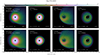 |
Fig. 5. Time-averaged GRRT decomposed images at 86 (top) and 43 GHz (bottom) with a black hole spin of a = 0.9375 using the reconnection heating model with an inclination angle of 163°. From left to right, the emissions come from every region: the whole region is depicted first, then the midplane, the nearside jet, and farside jet, respectively. The eDF of all of the images used is variable κ and the time-averaged total flux is 0.5 Jy at 230 GHz from t = 14 000 to 15 000 M. |
3.3. Image comparison
Following the previous study (Mizuno et al. 2021), to quantitatively compare the GRRT images obtained from the R − β models and the electron heating models, three image-comparison metrics were applied: the mean square error (MSE), the structural dissimilarity (DSSIM; Wang et al. 2004), and the difference of the normalized cross-correlation coefficient (NCCC) from 1; that is, 1-NCCC (Mizuno et al. 2018; Fromm et al. 2021).
For the total intensity emission of two images, I and J, the MSE was calculated pixel by pixel between two image pixels; namely,
 (6)
(6)
where Ik and Jk, are the intensity emission at the kth pixels of the two images, respectively. N is the total number of pixels of one image, assuming that both images have the same resolution.
Based on the human visual perception metric, the DSSIM, also known as the structural similarity index (SSIM), was calculated (Wang et al. 2004). The relation between them is DSSIM = 1/ |SSIM| − 1 and SSIM can be calculated as
 (7)
(7)
where  , and
, and  . The NCCC was computed as
 (8)
(8)
where ⟨I⟩ and ⟨J⟩ are average pixel values of Stokes intensity, and ΔI and ΔJ are standard deviations of pixel values (e.g., EHT Collaboration 2019d). Hence, the similarity between the two images is given by the value of NCCC, and thus NCCC = 1 denotes a strong correlation between the two images.
Image comparison between R − β models and electron heating models at 230 GHz, with variable κ and different black hole spins, adopting various quantitative comparison methods, are shown in Fig. 6. From t = 14 000 to 15 000 M, the snapshots of a R − β model are compared with the one with an electron heating model at the corresponding time for each 10 M. The lower value of the two models indicates a close match. The average values are represented in solid lines, while the shaded regions in the same color denote the standard deviation resulting from time variation, relative to the average values. The results indicate that all image-comparison metrics values show an overall upward trend with the increase in Rh values, although these values are relatively small. In other words, the GRRT images of the models with the smaller Rh values are more similar to the ones of the electron heating models at 230 GHz, without the dependency on black hole spins. This trend is the same as that seen in a previous study using thermal eDF (Mizuno et al. 2021), while we considered variable κ, and it is also consistent with recent results of self-consistent ion-to-electron temperature from PIC turbulent simulations (Meringolo et al. 2023). In most image-comparison metrics, the values of the counter-rotating cases (blue and green) have large standard deviations. Hence, it would be difficult to find to what extent a R − β model is comparable with the specified electron heating model. Besides, due to images at 230 GHz being already mostly optically thin, we also carried out a comparison of images at 86 GHz and 43 GHz and show the results in Appendix C. The aforementioned trend is also true even for lower frequencies. In addition, we also performed the same image comparison with the cases using nonthermal fixed κ = 3.5 eDF. For models with fixed κ = 3.5 eDF, the conclusion mentioned above does not change. Thus, this trend is independent of the eDFs.
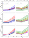 |
Fig. 6. Image comparison between R − β and electron heating models at different spins adopting various quantitative comparison methods with a 163° inclination angle at 230 GHz. From top to bottom: The comparison methods used are MSE, DSSIM, and 1-NCCC, respectively. From left to right, the prescriptions of electron heating models are turbulent and reconnection heating, respectively. The applied eDF is variable κ, and the time-averaged total flux is 0.5 Jy at 230 GHz. The colored dots and triangles represent average values from time variation at the specific spins, and the regions shaded in the same color denote the standard deviation relative to the average values. In all of the comparison methods, the lower value indicates a close match. |
Apart from that, we also explored the comparison for time-averaged images at each 50 M to mediate the effect of small temporal structures, using variable κ and fixed κ = 3.5 eDFs, at 230 GHz, 86 GHz, and 43 GHz. The results also support the aforementioned overall increase trend with increasing Rh values. The only exception is that the MSE and 1-NCCC metrics values decrease, especially for cases with higher Rh values. At the same time, DSSIM does not change significantly, compared with results using snapshot images. The possible reason may be that the location and brightness of the extended structures are more stable, while the bright emission near the photon ring dynamically changes faster. Hence, for cases with higher Rh values, the electron in the disk region is cooler, which lowers the luminosity of bright emission and makes a transitory structure the bigger disturbance in the region near the center, compared with lower Rh cases. Therefore, the DSSIM, which measures the similarity of the lower-flux regions, is not sensitive to time averaging due to dim extended structures being stable. For MSE and 1-NCCC, which are more weighted in the similarity of bright regions, they decrease due to the luminous instantaneous structures being offset by a time average. Notably, the net decrease in MSE and 1-NCCC in cases with higher Rh values is larger, since such an instantaneous structure is mitigated proportionally by a longer average time, which hints that the net values, if averaged for a longer time, are reduced more in cases with higher previous MSE or 1-NCCC values.
3.4. Spectral energy distribution
To investigate how flux varies with frequencies in different heating prescriptions, the SEDs with different electron heating models and distinct spins are shown in Fig. 7. The solid curves represent the average flux from t = 14 000 to t = 15 000 M, and the shaded regions denote the standard deviation resulting from the time variation, relative to the average values. Red, blue, and green curves correspond to the variable κ eDF cases using the electron heating prescription, the R − β model with Rh = 1, and the R − β model with Rh = 160, respectively. To exhibit the impact of nonthermal eDFs, as a reference, thermal eDF cases with electron heating prescriptions are added in Fig. 7 in black.
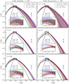 |
Fig. 7. Spectral energy distribution curves with different eDFs and different spins in turbulent heating (left) and reconnection heating (right) models. From top to bottom: black hole spins are −0.9375, 0, and 0.9375, respectively. The black curves adopt the thermal eDF, while the red curves employ variable κ eDF. For the comparison, variable κ eDF using the R − β model with Rh = 1 and 160 are presented as blue and green curves, respectively. The solid curves represent average values and the shaded regions denote the standard deviation relative to the average values. The dash-dotted vertical lines correspond to 43 GHz, 86 GHz, 230 GHz, and 136 THz. |
First, extracting entire features is helpful to better understand the behavior of SEDs as a whole. As is shown in Fig. 7, all of the curves behave similarly. As the frequency increases, the SED curves initially rise, followed by a decline after reaching the turnover frequency. This turnover frequency depends on both the magnetic field strength and electron temperature (Fromm et al. 2022). Since the time-averaged flux at 230 GHz was set to 0.5 Jy, all curves intersect at the same point. In all black hole spin cases, the standard deviation of the reconnection heating prescriptions is larger than that of turbulent heating, and the standard deviation of the R − β model with Rh = 1 is larger than that of the R − β model with Rh = 160. With a given electron heating prescription, the standard deviation of counter-rotating cases is the largest among cases with different black hole spins. A similar behavior was seen in the previous study (Mizuno et al. 2021).
Second, with the total flux fixed at 0.5 Jy at 230 GHz, the position of a peak that reflects the transition between optically thin and thick depends on the electron heating prescriptions and eDFs. For all black hole spin cases, the curve with variable κ eDF (red) reaches its peak at a slightly lower frequency than the one with a thermal eDF (black). The SED using the R − β model with Rh = 1 (blue) reaches its peak at a frequency comparatively lower than that using the R − β model with Rh = 160 (green). Thus, the peak position is sensitive to heating prescriptions.
Third, at high frequencies, the curves with electron heating prescriptions (black and red) and the curves with the R − β model with Rh = 1 (blue) behave similarly but the curves with the R − β model with Rh = 160 (green) deviate considerably from the other three models. Moreover, at high frequencies, within models with variable κ eDF, the flux of curves with Rh = 1 (blue) is slightly more luminous than that of turbulent heating but for reconnection heating the trend is opposite. Additionally, at high frequencies, the curves of electron heating prescriptions with variable κ eDF (red) have a marginally higher flux than those with thermal eDF (black). It reflects the truth that nonthermal electrons contribute more to the flux at higher frequencies (e.g., Davelaar et al. 2019; Cruz-Osorio et al. 2022; Fromm et al. 2022).
At low frequencies, the standard deviation becomes small due to lower time variability, and the variable κ eDF cases have a higher flux than those in the thermal eDF. It becomes possible to discern the electron heating models with variable κ eDF and those with thermal eDF through their SEDs.
In general, the contribution from the extended structure becomes larger in the emission at lower frequencies. In our studies, the FoV is limited to ±160 μas. Thus, we may underestimate the total flux in our SED at lower frequencies.
3.5. Time variability
The light curves at 230 GHz and 43 GHz of models with different spins, heating prescriptions, and eDFs are shown in Fig. 8. Generally, the global trend of flux variation over time is similar in both 230 GHz and 43 GHz. We also see some small variabilities in the R − β model with Rh = 160.
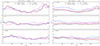 |
Fig. 8. Light curves of flux at 230 GHz (left) and 43 GHz (right) with a 163° inclination angle. Curves are plotted using a = −0.9375 (top), 0 (middle), and 0.9375 (bottom). The different colors correspond to the different heating prescriptions and eDFs: the turbulent heating model with thermal eDF (black), the turbulent heating model with variable κ eDf (red), the R − β model with Rh = 1 in variable κ eDF (blue), and the R − β model with Rh = 160 in variable κ (magenta). |
To quantitatively exhibit different behaviors of various models at different frequencies, the standard deviation of the time variability at 230 GHz and 43 GHz is shown in Fig. 9. At 230 GHz, we set the time-averaged flux at 0.5 Jy. Thus the average value is the same in all cases. However, the time-averaged flux at 43 GHz changes. In general, at 43 GHz, κ eDF cases have a larger flux than those of the thermal ones, and R − β models have a higher flux than those of the electron heating models. These are also seen in the SED profile in Figs. 7 and 8 for more clarity. In all heating models and eDFs, rotating black hole cases have higher variability than nonrotating cases and counter-rotating cases are more variable than corotating cases. It is a similar trend to that seen in the previous study (Mizuno et al. 2021). We do not see a clear difference in time variability between thermal and variable κ eDFs. This indicates that the properties of time variability do not depend on the eDFs.
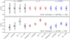 |
Fig. 9. Total flux variation in the turbulent heating model at 230 GHz (top) and 43 GHz (bottom). The different colors correspond to the different spins: a = −0.9375 (black), 0 (red), and 0.9375 (blue). The bottom labels denote the different heating prescriptions and eDFs: the turbulent heating model with thermal eDF (e-heating Th), the turbulent heating model with variable κ eDF (e-heating), the R − β model with Rh = 1 in variable κ eDF (Rh = 1), and the R − β model with Rh = 160 in variable κ eDF (Rh = 160). The colored dots represent average values from time variation in the specific models and the error bars denote the standard deviation relative to the average values (the number beside each error bar indicates the value of standard deviation normalized by the averaged value). |
3.6. Exclusion of magnetized region
Due to the density, pressure, and internal energy possibly reaching the floor value in simulations in highly magnetized regions (σ ≫ 1), it is necessary to choose a ceiling to exclude regions with strong magnetization (Chael et al. 2019). The conservative cut-off value σcut = 1 was chosen in the previous study with thermal eDF (Mizuno et al. 2021) and also in the previous results of this paper.
Here, we investigate the impacts of different σ thresholds on images, image comparison, SEDs, and total flux variation for a MAD state with a nonthermal eDF. Figure 10 shows the decomposed GRRT images with various σcut at 230 GHz with variable κ eDF. The results show that with σcut increasing to 10, the ratio of extended jet emission to total emission increases from 4.7% to 14.5%, compared to the case of σcut = 1. In the case with σcut = 10, there is a faint triple-ridged jet coming from the core, although this would be affected by our floor treatment in the diffuse high magnetization regions.
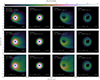 |
Fig. 10. From t = 14 000 to t = 15 000 M, time-averaged MAD GRRT decomposed images with a fixed black-hole spin of a = 0.9375 at 230 GHz. From top to bottom: images using σcut = 1, 2, and 10, respectively. From left to right, the emissions come from every region: the whole region is depicted first, then the midplane, the nearside jet, and the farside jet, respectively. The eDF of all of the images is variable κ, the electron heating prescription of all images is reconnection, and the time-averaged total flux of all of the images is 0.5 Jy at 230 GHz. |
Image comparison between R − β and electron heating models under different σcut adopting various quantitative comparison metrics are shown in Fig. 11. The results indicate that the R − β models could reproduce fairly well the images using electron heating models under different σcut. With the larger σcut values, the GRRT images of a R − β model are more similar to the ones of an electron heating model, although the increase in similarity is relatively small.
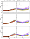 |
Fig. 11. Same as Fig. 6 at 230 GHz but with various exclusion of magnetized regions: σcut = 1 (black and dark violet), 2 (dark red and medium blue), 5 (red and green), and 10 (olive drab and dark orange). The black hole spin in all cases is a = 0.9375. |
For broadband spectral energy distributions, in variable κ eDF, the difference emerging from the choice of σcut is quite tiny up to 230 GHz. These results are consistent with those of thermal eDF (Mizuno et al. 2021). Thus, we skip to show the figure.
The dependency of the total flux variation on σcut is shown in Fig. 12. Overall, the variation in reconnection models is larger than that in turbulent heating models. Furthermore, with increasing σcut, the variation in the R − β model with Rh = 160 becomes smaller, while the difference between the two temperature models and the R − β model with Rh = 1 is small. Thus, the flux variation in these models does not have a dependence on σcut.
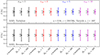 |
Fig. 12. Total flux variation of corotating cases in the turbulent heating model (top) and reconnection model (bottom) at 230 GHz. The different colors correspond to the different exclusions of magnetized regions: σcut = 1 (black), 2 (red), 5 (blue), and 10 (magenta). The labels at the bottom denote the different heating prescriptions: the electron heating model (e-heating), the R − β model with Rh = 1 (Rh = 1), and the R − β model with Rh = 160 (Rh = 160). The colored dots represent average values from time variation in the specific models and the error bars denote the standard deviation relative to the average values (the number beside each error bar indicates the value of standard deviation normalized by the averaged value). |
4. Summary and discussion
Previous research (Mizuno et al. 2021) has largely ignored the impacts of nonthermal electrons on the comparison of images between two-temperature electron heating and ordinary parameterized prescriptions. To address this issue, we adopted κ eDF (Davelaar et al. 2018, 2019), which can reproduce the power law tail and which has a thermal core. Using it, we have investigated the impacts of nonthermal eDFs on images, SEDs, and time variability at 230 GHz, 86 GHz, and 43 GHz with two various inclination angles (i = 163° and 60°). We have also explored the influence of different σ thresholds on the jet morphology, shadow images, SEDs, and total flux variation.
In a previous study (Mizuno et al. 2021), it was found that there is not much difference between the electron heating models and the R − β models using thermal distribution. In our study, at 230 GHz there is still no significant difference between electron heating models and the R − β models, even if nonthermal eDF is considered. In particular, independently of heating prescriptions and the σcut values, the R − β model with Rh = 1 is the most similar to the model with electron heating in terms of the morphological structure, and the SEDs at a high frequency.
From our results, the extent to which the diffuse extended jet contributes to the images is related to the eDFs, electron-heating mechanisms, frequencies, and the exclusion of magnetized regions. Specifically, images of the variable κ eDF are analogous to the thermal ones except for the small differences in the extended structure and the maximum flux. The edge-brightened jet emission structure is seen in the variable κ eDF in corotating black hole cases in magnetic reconnection heating. Through decomposed images, we have found that the emission coming from the nearside jet accounts for the origin of this edge-brightened jet and that it becomes more luminous at a lower frequency. To further investigate the contribution of the jet to total emission, the higher magnetized regions were also considered by increasing σcut from 1 to 10. The results show that with the growth of σcut the extended jet is more dominant. For instance, at 230 GHz, there will be 10% more emission coming from the jet if including the regions with magnetization 1 < σ < 10 when ε = 0. Moreover, if the magnetic energy contribution to κ eDF is considered (e.g., by setting ε = 0.5), 10% more emissions come from the jet contributed by electrons in magnetized regions (0 ≪ σ ≤ 1) with a radius larger than rinj = 10 M. In addition, the energy exchange due to Coulomb coupling, anisotropic heat flow conducted along magnetic field lines, and radiative cooling considered in previous work (Ressler et al. 2015, 2017; Chael et al. 2018, 2019) were ignored in our GRMHD simulation for simplicity. We should note that these effects will change the electron temperature distribution and the image morphology of the shadows; for instance, diffuse extended jets may become brighter (Chael et al. 2018; Dihingia et al. 2023).
In particular, from our results based on the images at lower frequencies, the extended emission contribution becomes larger. This finding suggests that nonthermal emission at lower frequencies such as 43 GHz and 86 GHz is more prominent, and such an extended jet mission has been seen in observations (EHT MWL Science Working Group 2021). Even with the images at 230 GHz that are explained sufficiently by the Maxwell-Jüttner distribution (EHT Collaboration 2019e), the nonthermal contribution is crucial to explaining enough emission from the extended jet at other frequencies. For instance, nonthermal eDF could reproduce the emission structure of M87 at 86 GHz (Cruz-Osorio et al. 2022; Yang et al. 2024). Moreover, future multi-frequency observations are needed to investigate the electron heating mechanism for the production of the emission of black hole shadows and extended diffuse jets. Observation of the potential faint jet structure at 230 GHz is crucial to imposing additional restrictions on models. Indeed, future observations at 230 GHz from space (Doeleman et al. 2019; Raymond et al. 2021; Roelofs et al. 2021) are expected to detect this faint extended structure. Recently, Fromm et al. (in prep.) have studied the possibility of determining the electron heating model by SED and spectral index maps from the observations of future VLBI arrays.
Lastly, we note that, in this work, we only investigated the MAD model. In general, images created from the SANE model have more dependency for the choice of Rh value. Future research should study the SANE model to make our conclusion more robust.
Acknowledgments
This research is supported by the National Key R&D Program of China (2023YFE0101200), the National Natural Science Foundation of China (Grant No. 12273022), and the Shanghai Municipality orientation program of Basic Research for International Scientists (Grant No. 22JC1410600). C.M.F. is supported by the DFG research grant “Jet physics on horizon scales and beyond” (Grant No. 443220636). Z.Y. acknowledges support from a UKRI Stephen Hawking Fellowship. A.C.O. gratefully acknowledges “Ciencia Básica y de Frontera 2023-2024” program of the “Consejo Nacional de Humanidades, Ciencias y Tecnología” (CONAHCYT, México), projects CBF2023-2024-1102 and 257435. The simulations were performed on the Astro cluster in Tsung-Dao Lee Institute, π 2.0, and Siyuan-1 cluster in the Center for High Performance Computing at Shanghai Jiao Tong University. This work has made use of NASA’s Astrophysics Data System (ADS).
References
- Ball, D., Sironi, L., & Özel, F. 2018, ApJ, 862, 80 [Google Scholar]
- Blandford, R. D., & Znajek, R. L. 1977, MNRAS, 179, 433 [NASA ADS] [CrossRef] [Google Scholar]
- Bower, G. C., Wright, M. C. H., Falcke, H., & Backer, D. C. 2003, ApJ, 588, 331 [Google Scholar]
- Bower, G. C., Goss, W. M., Falcke, H., Backer, D. C., & Lithwick, Y. 2006, ApJ, 648, L127 [NASA ADS] [CrossRef] [Google Scholar]
- Broderick, A. E., & Loeb, A. 2009, ApJ, 697, 1164 [NASA ADS] [CrossRef] [Google Scholar]
- Chael, A., Rowan, M., Narayan, R., Johnson, M., & Sironi, L. 2018, MNRAS, 478, 5209 [NASA ADS] [CrossRef] [Google Scholar]
- Chael, A., Narayan, R., & Johnson, M. D. 2019, MNRAS, 486, 2873 [NASA ADS] [CrossRef] [Google Scholar]
- Cruz-Osorio, A., Fromm, C. M., Mizuno, Y., et al. 2022, Nat. Astron., 6, 103 [NASA ADS] [CrossRef] [Google Scholar]
- Cunningham, C. T., & Bardeen, J. M. 1973, ApJ, 183, 237 [Google Scholar]
- Damour, T., & Polyakov, A. M. 1994, Nucl. Phys. B, 423, 532 [Google Scholar]
- Davelaar, J., Mościbrodzka, M., Bronzwaer, T., & Falcke, H. 2018, A&A, 612, A34 [NASA ADS] [CrossRef] [EDP Sciences] [Google Scholar]
- Davelaar, J., Olivares, H., Porth, O., et al. 2019, A&A, 632, A2 [NASA ADS] [CrossRef] [EDP Sciences] [Google Scholar]
- Davelaar, J., Ripperda, B., Sironi, L., et al. 2023, ApJ, 959, L3 [NASA ADS] [CrossRef] [Google Scholar]
- De Villiers, J.-P., & Hawley, J. F. 2003, ApJ, 589, 458 [NASA ADS] [CrossRef] [Google Scholar]
- Dexter, J., Agol, E., Fragile, P. C., & McKinney, J. C. 2010, ApJ, 717, 1092 [NASA ADS] [CrossRef] [Google Scholar]
- Dihingia, I. K., Mizuno, Y., Fromm, C. M., & Younsi, Z. 2023, ArXiv e-prints [arXiv:2305.09698] [Google Scholar]
- Ding, J., Yuan, F., & Liang, E. 2010, ApJ, 708, 1545 [NASA ADS] [CrossRef] [Google Scholar]
- Doeleman, S., Blackburn, L., Dexter, J., et al. 2019, BAAS, 51, 256 [Google Scholar]
- EHT Collaboration (Alberdi, A., et al.) 2019a, ApJ, 875, L1 [NASA ADS] [CrossRef] [Google Scholar]
- EHT Collaboration (Alberdi, A., et al.) 2019b, ApJ, 875, L2 [NASA ADS] [CrossRef] [Google Scholar]
- EHT Collaboration (Alberdi, A., et al.) 2019c, ApJ, 875, L3 [NASA ADS] [CrossRef] [Google Scholar]
- EHT Collaboration (Alberdi, A., et al.) 2019d, ApJ, 875, L4 [CrossRef] [Google Scholar]
- EHT Collaboration (Alberdi, A., et al.) 2019e, ApJ, 875, L5 [NASA ADS] [CrossRef] [Google Scholar]
- EHT Collaboration (Alberdi, A., et al.) 2019f, ApJ, 875, L6 [NASA ADS] [CrossRef] [Google Scholar]
- EHT MWL Science Working Group (Algaba, J. C., et al.) 2021, ApJ, 911, L11 [NASA ADS] [CrossRef] [Google Scholar]
- Fromm, C. M., Mizuno, Y., Younsi, Z., et al. 2021, A&A, 649, A116 [NASA ADS] [CrossRef] [EDP Sciences] [Google Scholar]
- Fromm, C. M., Cruz-Osorio, A., Mizuno, Y., et al. 2022, A&A, 660, A107 [NASA ADS] [CrossRef] [EDP Sciences] [Google Scholar]
- Grenzebach, A., Perlick, V., & Lämmerzahl, C. 2014, Phys. Rev. D, 89, 124004 [NASA ADS] [CrossRef] [Google Scholar]
- Ho, L. C. 2009, ApJ, 699, 626 [NASA ADS] [CrossRef] [Google Scholar]
- Hoshino, M. 2013, ApJ, 773, 118 [Google Scholar]
- Jiang, H.-X., Mizuno, Y., Fromm, C. M., & Nathanail, A. 2023, MNRAS, 522, 2307 [NASA ADS] [CrossRef] [Google Scholar]
- Kawazura, Y., Barnes, M., & Schekochihin, A. A. 2019, Proc. Natl. Acad. Sci., 116, 771 [NASA ADS] [CrossRef] [Google Scholar]
- Komissarov, S. S. 1999, MNRAS, 303, 343 [NASA ADS] [CrossRef] [Google Scholar]
- Kunz, M. W., Stone, J. M., & Quataert, E. 2016, Phys. Rev. Lett., 117, 235101 [NASA ADS] [CrossRef] [Google Scholar]
- Kuo, C. Y., Asada, K., Rao, R., et al. 2014, ApJ, 783, L33 [NASA ADS] [CrossRef] [Google Scholar]
- Marrone, D. P., Moran, J. M., Zhao, J.-H., & Rao, R. 2007, ApJ, 654, L57 [NASA ADS] [CrossRef] [Google Scholar]
- Meringolo, C., Cruz-Osorio, A., Rezzolla, L., & Servidio, S. 2023, ApJ, 944, 122 [NASA ADS] [CrossRef] [Google Scholar]
- Mizuno, Y., Younsi, Z., Fromm, C. M., et al. 2018, Nat. Astron., 2, 585 [Google Scholar]
- Mizuno, Y., Fromm, C. M., Younsi, Z., et al. 2021, MNRAS, 506, 741 [NASA ADS] [CrossRef] [Google Scholar]
- Moriyama, K., Cruz-Osorio, A., Mizuno, Y., et al. 2024, ApJ, 960, 106 [NASA ADS] [CrossRef] [Google Scholar]
- Mościbrodzka, M., Gammie, C. F., Dolence, J. C., Shiokawa, H., & Leung, P. K. 2009, ApJ, 706, 497 [Google Scholar]
- Mościbrodzka, M., Falcke, H., Shiokawa, H., & Gammie, C. F. 2014, A&A, 570, A7 [Google Scholar]
- Mościbrodzka, M., Falcke, H., & Shiokawa, H. 2016, A&A, 586, A38 [Google Scholar]
- Nakamura, M., Asada, K., Hada, K., et al. 2018, ApJ, 868, 146 [Google Scholar]
- Narayan, R., & Yi, I. 1995, ApJ, 444, 231 [Google Scholar]
- Narayan, R., Igumenshchev, I. V., & Abramowicz, M. A. 2003, PASJ, 55, L69 [NASA ADS] [Google Scholar]
- Narayan, R., Sądowski, A., Penna, R. F., & Kulkarni, A. K. 2012, MNRAS, 426, 3241 [Google Scholar]
- Noble, S. C., Leung, P. K., Gammie, C. F., & Book, L. G. 2007, Class. Quant. Grav., 24, S259 [NASA ADS] [CrossRef] [Google Scholar]
- Olivares, H., Porth, O., Davelaar, J., et al. 2019, A&A, 629, A61 [NASA ADS] [CrossRef] [EDP Sciences] [Google Scholar]
- Olivares Sánchez, H., Porth, O., & Mizuno, Y. 2018, J. Phys. Conf. Ser., 1031, 012008 [CrossRef] [Google Scholar]
- Pandya, A., Zhang, Z., Chandra, M., & Gammie, C. F. 2016, ApJ, 822, 34 [Google Scholar]
- Porth, O., Olivares, H., Mizuno, Y., et al. 2017, Comput. Astrophys. Cosmol., 4, 1 [Google Scholar]
- Prieto, M. A., Fernández-Ontiveros, J. A., Markoff, S., Espada, D., & González-Martín, O. 2016, MNRAS, 457, 3801 [NASA ADS] [CrossRef] [Google Scholar]
- Raymond, A. W., Palumbo, D., Paine, S. N., et al. 2021, ApJS, 253, 5 [Google Scholar]
- Ressler, S. M., Tchekhovskoy, A., Quataert, E., Chandra, M., & Gammie, C. F. 2015, MNRAS, 454, 1848 [Google Scholar]
- Ressler, S. M., Tchekhovskoy, A., Quataert, E., & Gammie, C. F. 2017, MNRAS, 467, 3604 [NASA ADS] [CrossRef] [Google Scholar]
- Ricarte, A., Gammie, C., Narayan, R., & Prather, B. S. 2023, MNRAS, 519, 4203 [NASA ADS] [CrossRef] [Google Scholar]
- Roelofs, F., Fromm, C. M., Mizuno, Y., et al. 2021, A&A, 650, A56 [NASA ADS] [CrossRef] [EDP Sciences] [Google Scholar]
- Rowan, M. E., Sironi, L., & Narayan, R. 2017, ApJ, 850, 29 [NASA ADS] [CrossRef] [Google Scholar]
- Shcherbakov, R. V., Penna, R. F., & McKinney, J. C. 2012, ApJ, 755, 133 [NASA ADS] [CrossRef] [Google Scholar]
- Sądowski, A., Narayan, R., Penna, R., & Zhu, Y. 2013, MNRAS, 436, 3856 [Google Scholar]
- Tchekhovskoy, A., Narayan, R., & McKinney, J. C. 2011, MNRAS, 418, L79 [NASA ADS] [CrossRef] [Google Scholar]
- Vasyliunas, V. M. 1968, J. Geophys. Res., 73, 2839 [NASA ADS] [CrossRef] [Google Scholar]
- Wang, Z., Bovik, A. C., Sheikh, H. R., & Simoncelli, E. P. 2004, IEEE Trans. Image Process., 13, 600 [Google Scholar]
- Xiao, F. 2006, Plasma Phys. Control. Fusion, 48, 203 [NASA ADS] [CrossRef] [Google Scholar]
- Yang, H., Yuan, F., Li, H., et al. 2024, Sci. Adv., 10, eadn3544 [NASA ADS] [CrossRef] [Google Scholar]
- Younsi, Z., Wu, K., & Fuerst, S. V. 2012, A&A, 545, A13 [NASA ADS] [CrossRef] [EDP Sciences] [Google Scholar]
- Younsi, Z., Zhidenko, A., Rezzolla, L., Konoplya, R., & Mizuno, Y. 2016, Phys. Rev. D, 94, 084025 [Google Scholar]
- Younsi, Z., Porth, O., Mizuno, Y., Fromm, C. M., Olivares, H. 2020, in Perseus in Sicily: From Black Hole to Cluster Outskirts, eds. K. Asada, E. de Gouveia Dal Pino, M. Giroletti, H. Nagai, & R. Nemmen, 342, 9 [NASA ADS] [Google Scholar]
- Younsi, Z., Psaltis, D., & Özel, F. 2023, ApJ, 942, 47 [NASA ADS] [CrossRef] [Google Scholar]
- Yuan, F., & Narayan, R. 2014, ARA&A, 52, 529 [NASA ADS] [CrossRef] [Google Scholar]
Appendix A: The effect of the magnetic energy contribution to the κ width, w
To investigate the effect of the magnetic energy contribution to the width, w, of the κ distribution at different frequencies, we performed the GRRT calculation using variable κ and set ε = 0.5 in Eq. (3). As is shown in Fig. A.1, the emission originating from nearside jet accounts for 13.6% of the total emission at 230 GHz and reaches 24.4% at 43 GHz. It shows that the contribution from the nearside jet emission increases at lower frequencies, which is consistent with the trend we found in Fig. 3 and Fig. 4, in which ε = 0. However, there is a constant enhancement of around 10% on the nearside jet at these three frequencies, compared with the results using ε = 0. To imagine how the κ width, w, of the κ distribution in Eq. (3) distributes around the black hole, Figure A.2 shows the time and azimuthally averaged width, w, of the κ distribution with ε = 0 and 0.5. In the case of the width, w, with ε = 0, it does not consider the contribution of magnetic energy in highly magnetized regions; that is, the jet sheath region. When considering a nonzero ε case such as ε = 0.5, the w is significantly enhanced for those regions with a radius larger than rinj = 10 M and σ > 1, and the w is also enhanced for those magnetized regions (0 ≪ σ ≤ 1) with a radius larger than rinj = 10 M. Therefore, more emissions come from the jet, and the extended structure becomes more luminous. Due to the total flux being fixed, the portion of emission coming from the nearside jet increases at different frequencies.
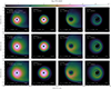 |
Fig. A.1. Time-averaged GRRT decomposed images at 230 (top), 86 (middle), and 43 GHz (bottom) with a black hole spin of a = 0.9375 using the reconnection heating model with an inclination angle of 163°. From left to right, the emissions come from every region: the whole region is depicted first, then the midplane, the nearside jet, and the farside jet, respectively. The eDF of all of the images used is variable κ with ε = 0.5 in the κ width, w, and the time-averaged total flux is 0.5 Jy at 230 GHz from t = 14 000 to 15 000 M. |
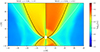 |
Fig. A.2. Time and azimuthally averaged width, w, of the κ distribution on a logarithmic scale, with the reconnection heating prescription (a = 0.94). The left panel shows the width, w, with ε = 0, and the right one shows the nonzero ε model with ε = 0.5. The solid black and dashed white lines represent σ = 1 and the Bernoulli parameter, −hut = 1.02, respectively. |
Appendix B: Decomposed images at inclination 60°
As is shown in Fig. 3, the images using reconnection heating lead to a smaller vertical extended structure at an inclination angle of 60°, in contrast with the ones of the turbulent heating or the R − β prescriptions. To understand the origin of this vertically extended structure, we calculated the decomposed images following the same procedure as in Fig. 4. We should note that the accretion rates for the calculation of images at 60° are the same as those at 163°. The results with black hole spin a = 0.9375 are shown in Fig. B.1. Because the decomposed images are calculated by the limitation of the simulation domain, the emission from the equatorial plane is omitted for nearside and farside images, which are shown as vertical discontinuous dark areas in those images. Clearly, the turbulent model results in a vertically extended structure, compared with the reconnection model. As is seen in the decomposed images at 163° (Fig. 4), emission from midplane in the turbulent heating model is more dominant than those in the reconnection heating model. Such a difference is enhanced as the difference of vertically extended structure in the images at 60°.
Appendix C: Image comparison at 86 and 43 GHz
Due to the images at 230 GHz being almost optically thin, it is useful to investigate how the similarity between R − β model and two-temperature models varies with Rh values at lower frequencies. To do it, we performed a snapshot image comparison between the two-temperature electron heating model and R − β model with different Rh at 86 GHz and 43 GHz. Figure C.1 provides the quantitative image comparison at 86 GHz and 43 GHz, using three different metrics described in section 3.3. Smaller values indicate more similarity between the two corresponding compared models. The results also indicate that all of the image-comparison metric values exhibit an overall increasing trend with the increase in Rh values. In addition, the DSSIM values become higher at lower frequencies, which hints that there is more divergence of diffuse, extended structures between R − β models and electron heating models at lower frequencies.
Appendix D: The equilibrium radius of general relativistic magnetohydrodynamic simulations
As was mentioned in Sec. 2.1, the GRMHD simulations reach a quasi-stationary state at t = 15 000 M, and thereafter we discussed the impacts of nonthermal distribution on GRRT images based on these GRMHD data. Typically, a longer simulation time provides sufficient time for the accretion flows to reach the equilibrium state with a larger radius. To confirm that the nonthermal extended emission stems from the relaxation region rather than the regions with very large radii, where there the equilibrium state at t = 15 000 M has still not yet been reached, it is necessary to provide convincing proof of the relaxation of these GRMHD simulations up to a desired radius at t = 15 000 M. Figure D.1 provides the time-averaged vertically integrated mass flux ( , where g is the metric determinant, ρ is the fluid rest-mass density, and ur is the radial component of the 4-velocity) as a function of the radius for different spin cases using the turbulent heating prescription. The net mass flux of inflow and outflow is integrated over θ from 0 to π for a given radius, and this value will reach a constant for those regions when it reaches the equilibrium. In the nonrotating and corotating black hole cases, even at t = 15 000 M, Figure D.1 shows that they have reached an equilibrium at the radius greater than the current FoV of the GRRT images (∼40 M). In counter-rotating cases, since the ISCO position, RISCO ≈ 8.8 M, is far from the black hole horizon, it takes more time to reach the equilibrium state for a given radius. However, for current GRRT images, almost all emissions are coming within 120 μas, which corresponds to 31.6 M, and within this radius all cases reach an equilibrium state. For cases using the reconnection heating prescription, the discussion of equilibrium radius is similar, and we only discuss the turbulent cases here for simplicity.
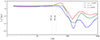 |
Fig. D.1. Time-averaged vertically integrated mass flux with black hole spins of a = −0.9375 (red), 0 (green), and 0.9375 (blue) in the turbulent heating prescription. The dash-dotted vertical lines correspond to the apparent radius of 120 and 160 μas FoV in the GRRT images. |
All Figures
|
Fig. 1. Time-averaged GRRT images of MAD simulations with various black hole spins and eDFs at 230 GHz with an inclination angle of 163°. From top to bottom: black hole spins with a = −0.9375, 0, and 0.9375, respectively. From left to right: the variable κ eDF using the R − β model with Rh = 1, turbulent and reconnection heating, and a fixed κ eDF, with κ = 3.5 using the R − β model with Rh = 1, turbulent and reconnection heating prescriptions. The dashed white contour indicates the curve with 1% of the maximum flux. The time-averaged total flux is 0.5 Jy at 230 GHz, with a simulation time span from t = 14 000 to 15 000 M. |
| In the text | |
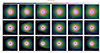 |
Fig. 2. Same as Fig. 1 but shown in 86 GHz. |
| In the text | |
|
Fig. 3. Time-averaged GRRT images of MAD simulations with a black hole spin of a = 0.9375 at 230 GHz and an inclination angle of 60°. From top to bottom: the eDF models using thermal, fixed κ = 3.5, and variable κ, respectively. From left to right: electron heating prescriptions using reconnection heating, turbulent heating, and the R − β model with Rh = 1 and Rh = 160, respectively. The dashed white contour indicates the curve with 1% of the maximum flux. The time-averaged total flux is 0.5 Jy from t = 14 000 to 15 000 M at 163°. |
| In the text | |
|
Fig. 4. Time-averaged GRRT decomposed images with a black hole spin of a = 0.9375 at 230 GHz with a 163° inclination angle. From top to bottom: images using the R − β model with Rh = 1, the turbulent heating model, and the reconnection heating model, respectively. From left to right, the emissions come from every region: the whole region is depicted first, then the midplane, the nearside jet, and the farside jet, respectively. The eDF of all of the images is variable κ and the time-averaged total flux is 0.5 Jy at 230 GHz from t = 14 000 to 15 000 M. |
| In the text | |
|
Fig. 5. Time-averaged GRRT decomposed images at 86 (top) and 43 GHz (bottom) with a black hole spin of a = 0.9375 using the reconnection heating model with an inclination angle of 163°. From left to right, the emissions come from every region: the whole region is depicted first, then the midplane, the nearside jet, and farside jet, respectively. The eDF of all of the images used is variable κ and the time-averaged total flux is 0.5 Jy at 230 GHz from t = 14 000 to 15 000 M. |
| In the text | |
|
Fig. 6. Image comparison between R − β and electron heating models at different spins adopting various quantitative comparison methods with a 163° inclination angle at 230 GHz. From top to bottom: The comparison methods used are MSE, DSSIM, and 1-NCCC, respectively. From left to right, the prescriptions of electron heating models are turbulent and reconnection heating, respectively. The applied eDF is variable κ, and the time-averaged total flux is 0.5 Jy at 230 GHz. The colored dots and triangles represent average values from time variation at the specific spins, and the regions shaded in the same color denote the standard deviation relative to the average values. In all of the comparison methods, the lower value indicates a close match. |
| In the text | |
|
Fig. 7. Spectral energy distribution curves with different eDFs and different spins in turbulent heating (left) and reconnection heating (right) models. From top to bottom: black hole spins are −0.9375, 0, and 0.9375, respectively. The black curves adopt the thermal eDF, while the red curves employ variable κ eDF. For the comparison, variable κ eDF using the R − β model with Rh = 1 and 160 are presented as blue and green curves, respectively. The solid curves represent average values and the shaded regions denote the standard deviation relative to the average values. The dash-dotted vertical lines correspond to 43 GHz, 86 GHz, 230 GHz, and 136 THz. |
| In the text | |
|
Fig. 8. Light curves of flux at 230 GHz (left) and 43 GHz (right) with a 163° inclination angle. Curves are plotted using a = −0.9375 (top), 0 (middle), and 0.9375 (bottom). The different colors correspond to the different heating prescriptions and eDFs: the turbulent heating model with thermal eDF (black), the turbulent heating model with variable κ eDf (red), the R − β model with Rh = 1 in variable κ eDF (blue), and the R − β model with Rh = 160 in variable κ (magenta). |
| In the text | |
|
Fig. 9. Total flux variation in the turbulent heating model at 230 GHz (top) and 43 GHz (bottom). The different colors correspond to the different spins: a = −0.9375 (black), 0 (red), and 0.9375 (blue). The bottom labels denote the different heating prescriptions and eDFs: the turbulent heating model with thermal eDF (e-heating Th), the turbulent heating model with variable κ eDF (e-heating), the R − β model with Rh = 1 in variable κ eDF (Rh = 1), and the R − β model with Rh = 160 in variable κ eDF (Rh = 160). The colored dots represent average values from time variation in the specific models and the error bars denote the standard deviation relative to the average values (the number beside each error bar indicates the value of standard deviation normalized by the averaged value). |
| In the text | |
|
Fig. 10. From t = 14 000 to t = 15 000 M, time-averaged MAD GRRT decomposed images with a fixed black-hole spin of a = 0.9375 at 230 GHz. From top to bottom: images using σcut = 1, 2, and 10, respectively. From left to right, the emissions come from every region: the whole region is depicted first, then the midplane, the nearside jet, and the farside jet, respectively. The eDF of all of the images is variable κ, the electron heating prescription of all images is reconnection, and the time-averaged total flux of all of the images is 0.5 Jy at 230 GHz. |
| In the text | |
|
Fig. 11. Same as Fig. 6 at 230 GHz but with various exclusion of magnetized regions: σcut = 1 (black and dark violet), 2 (dark red and medium blue), 5 (red and green), and 10 (olive drab and dark orange). The black hole spin in all cases is a = 0.9375. |
| In the text | |
|
Fig. 12. Total flux variation of corotating cases in the turbulent heating model (top) and reconnection model (bottom) at 230 GHz. The different colors correspond to the different exclusions of magnetized regions: σcut = 1 (black), 2 (red), 5 (blue), and 10 (magenta). The labels at the bottom denote the different heating prescriptions: the electron heating model (e-heating), the R − β model with Rh = 1 (Rh = 1), and the R − β model with Rh = 160 (Rh = 160). The colored dots represent average values from time variation in the specific models and the error bars denote the standard deviation relative to the average values (the number beside each error bar indicates the value of standard deviation normalized by the averaged value). |
| In the text | |
|
Fig. A.1. Time-averaged GRRT decomposed images at 230 (top), 86 (middle), and 43 GHz (bottom) with a black hole spin of a = 0.9375 using the reconnection heating model with an inclination angle of 163°. From left to right, the emissions come from every region: the whole region is depicted first, then the midplane, the nearside jet, and the farside jet, respectively. The eDF of all of the images used is variable κ with ε = 0.5 in the κ width, w, and the time-averaged total flux is 0.5 Jy at 230 GHz from t = 14 000 to 15 000 M. |
| In the text | |
|
Fig. A.2. Time and azimuthally averaged width, w, of the κ distribution on a logarithmic scale, with the reconnection heating prescription (a = 0.94). The left panel shows the width, w, with ε = 0, and the right one shows the nonzero ε model with ε = 0.5. The solid black and dashed white lines represent σ = 1 and the Bernoulli parameter, −hut = 1.02, respectively. |
| In the text | |
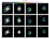 |
Fig. B.1. Same as Fig. 4 but with an inclination angle of 60°. |
| In the text | |
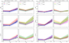 |
Fig. C.1. Same as Fig. 6 but at 86 GHz (left) and 43 GHz (right). |
| In the text | |
|
Fig. D.1. Time-averaged vertically integrated mass flux with black hole spins of a = −0.9375 (red), 0 (green), and 0.9375 (blue) in the turbulent heating prescription. The dash-dotted vertical lines correspond to the apparent radius of 120 and 160 μas FoV in the GRRT images. |
| In the text | |
Current usage metrics show cumulative count of Article Views (full-text article views including HTML views, PDF and ePub downloads, according to the available data) and Abstracts Views on Vision4Press platform.
Data correspond to usage on the plateform after 2015. The current usage metrics is available 48-96 hours after online publication and is updated daily on week days.
Initial download of the metrics may take a while.