| Issue |
A&A
Volume 694, February 2025
|
|
|---|---|---|
| Article Number | A135 | |
| Number of page(s) | 11 | |
| Section | Numerical methods and codes | |
| DOI | https://doi.org/10.1051/0004-6361/202452679 | |
| Published online | 07 February 2025 | |
Black hole accretion and radiation variability in general relativistic magnetohydrodynamic simulations with Rezzolla–Zhidenko spacetime
1
Instituto de Astrofísica de Andalucía-CSIC, Glorieta de la Astronomía s/n,
18008
Granada,
Spain
2
Institut für Theoretische Physik, Goethe-Universität Frankfurt,
Max-von-Laue-Strasse 1,
60438
Frankfurt am Main,
Germany
3
Mizusawa VLBI Observatory, National Astronomical Observatory of Japan,
2-12 Hoshigaoka, Mizusawa, Oshu,
Iwate
023-0861,
Japan
4
Instituto de Astronomía, Universidad Nacional Autónoma de México,
AP 70-264,
Ciudad de México
04510,
Mexico
5
Tsung-Dao Lee Institute, Shanghai Jiao Tong University,
No.1 Lisuo Road,
Shanghai
201210,
PR China
6
School of Physics and Astronomy, Shanghai Jiao Tong University,
800 Dongchuan Road,
Shanghai
200240,
PR China
★ Corresponding authors; moriyama@iaa.es; aosorio@astro.unam.mx
Received:
20
October
2024
Accepted:
10
January
2025
The Event Horizon Telescope (EHT) has unveiled the horizon-scale radiation properties of Sagittarius A* (Sgr A*), the supermassive black hole at the center of our galaxy, providing a novel platform for testing gravitational theories by comparing observations with theoretical models. A key next step is to investigate the nature of accretion flows and spacetime structures near black holes by analyzing the time variability observed in EHT data alongside general relativistic magnetohydrodynamic (GRMHD) simulations. We explored the dynamics of accretion flows in spherically symmetric black hole spacetimes with deviations from general relativity utilizing two dimensional GRMHD simulations based on the Rezzolla–Zhidenko parameterized spacetime. This study marks the first systematic investigation into how variability amplitudes in light curves, derived from non-Kerr GRMHD simulations, depend on deviations from the Schwarzschild spacetime. The deviation parameters are consistent with the constraints from weak gravitational fields and the size of Sgr A*’s black hole shadow. We find that the dynamics of accretion flows systematically depend on these parameters. In spacetimes with a deeper gravitational potential, fluid and Alfvén velocities consistently decrease relative to the Schwarzschild metric, indicating weaker dynamical behavior. We also examined the influence of spacetime deviations on radiation properties by computing luminosity fluctuations at 230 GHz using general relativistic radiative transfer simulations, in line with EHT observations. The amplitude of these fluctuations exhibits a systematic dependence on the deviation parameters, decreasing for deeper gravitational potentials compared to the Schwarzschild metric. These features are validated using one of the theoretically predicted metrics, the Hayward metric, a model that describes nonsingular black holes. This characteristic is expected to have similar effects in more comprehensive simulations that include more realistic accretion disk models and electron cooling in the future, potentially aiding in distinguishing black hole solutions that explain the variability of Sgr A*.
Key words: black hole physics / gravitation / hydrodynamics / magnetohydrodynamics (MHD) / radiative transfer
© The Authors 2025
 Open Access article, published by EDP Sciences, under the terms of the Creative Commons Attribution License (https://creativecommons.org/licenses/by/4.0), which permits unrestricted use, distribution, and reproduction in any medium, provided the original work is properly cited.
This article is published in open access under the Subscribe to Open model. Subscribe to A&A to support open access publication.
1 Introduction
Investigating the horizon-scale emission near the black hole is crucial, offering essential observational insights into the black hole spacetime and serving as a fundamental test of general relativity. Recently, the Event Horizon Telescope (EHT) Collaboration released the first horizon-scale images of the supermassive black hole at our galaxy’s center, Sagittarius A* (Sgr A*), and in the nearby radio galaxy M87 (Event Horizon Telescope Collaboration 2019a, 2022a). Each image shows ring morphology with diameters and structures that are consistent with the predictions of general relativity. Notably, Sgr A*, the main subject of this manuscript, is one of the most promising sources of all the EHT targets due to its unique properties: (1) it has the largest apparent size of the event horizon (∼50 µas; Event Horizon Telescope Collaboration 2022c,d), (2) its comparatively low mass produces rapid time variability events (e.g., IR/X- ray flares) with orbital timescales as short as 4–30 minutes, depending on the black hole spin (e.g., Baganoff et al. 2001; Marrone et al. 2008; Dodds-Eden et al. 2009; Gillessen et al. 2009; Yusef-Zadeh et al. 2009; Neilsen et al. 2013), and (3) the precise a priori measurements of its mass and distance (Do et al. 2019; GRAVITY Collaboration 2019).
The radius and asymmetry of the black hole shadow provide insights into the spacetime structure in the vicinity of the black hole. According to general relativity, the structure of the black hole spacetime is described by the Kerr metric, characterized by the mass (M) and the normalized black hole spin (Kerr 1963). The size and asymmetry of the black hole shadow are determined by the spacetime geometry, the black hole’s distance from Earth, and the viewing angle, with various alternative gravity theories offering precise solutions for the shadow’s morphology (e.g., see Younsi et al. 2016; Vagnozzi et al. 2023). In particular, Event Horizon Telescope Collaboration (2022b) has provided state-of-the-art results for observationally constraining deviations from the Schwarzschild metric (Kerr metric for a non-spinning black hole) using Sgr A* horizon-scale imaging, thereby establishing the confidence regime for the deviation parameters. Furthermore, Vagnozzi et al. (2023) provide a comprehensive survey that takes a wide range of well-motivated deviations from black hole solutions of general relativity into consideration. These theoretical milestones have led to a continuous series of related papers exploring the research on black hole shadows and alternative spacetime (e.g., Cruz-Osorio et al. 2021; Walia et al. 2022; Pantig & Övgün 2023; Sengo et al. 2023; Uniyal et al. 2023; Kocherlakota et al. 2024; Övgün et al. 2024; Paul et al. 2024).
Despite recent observational and theoretical progress, accurately measuring the Sgr A* black hole spacetime requires achieving additional main milestones: improving the observational accuracy of the ring radius and constructing theoretical simulations whose radiation variability is consistent with that of Sgr A*. According to general relativity, the diameter of the black hole shadow is predicted to depend weakly on the observer’s inclination angle and the black hole spin, approximately 𝒟 = 5.0 ± 0.2 rg, where rg = GM/c2 is the gravitational radius, G is the gravitational constant, and c is the speed of light (e.g., see Takahashi 2004; Chan et al. 2013; Event Horizon Telescope Collaboration 2022b). While the radius measurement has provided constraints on the parameters of each black hole spacetime according to some alternative theories, the slight difference in the shadow’s size compared to predictions from general relativity remains challenging to detect given the current angular resolution of EHT observations (approximately 20 µas, equivalent to around 4rg). Currently, continuous research is exploring possible methodologies for achieving accurate shadow size estimates and placing tight constraints on spacetime, especially focusing on expected future observational improvements, such as planned EHT observations, next-generation EHT (ngEHT), and the Black Hole Explorer (BHEX) projects (e.g., Gralla et al. 2019; Himwich et al. 2020; Johnson et al. 2020; Gurvits et al. 2022; Palumbo & Wong 2022; Chael et al. 2023; Kocherlakota et al. 2024).
Event Horizon Telescope Collaboration (2022e) compared the Sgr A* data observed by the EHT in 2017, along with data from other wavelengths (86 GHz, 136 THz, and X-rays), with theoretical models based on general relativistic magnetohydrodynamic (GRMHD) simulations and general relativistic radiation transfer (GRRT) simulations. They conducted theoretical GRMHD simulations, including the magnetically arrested disk (MAD; e.g., Igumenshchev et al. 2003; Narayan et al. 2003; Tchekhovskoy et al. 2011; McKinney et al. 2012), standard and normal evolution (SANE; e.g., Narayan et al. 2012; Sądowski et al. 2013), and tilted disk models with various parameters (e.g., Liska et al. 2018; Chatterjee et al. 2020), as well as a stellar wind-fed model with limited parameters (e.g., Ressler et al. 2018, 2020a,b). The radiation properties were then calculated based on the synchrotron radiation using both thermal and nonthermal electron distributions and compared with observational data. This sophisticated observational evidence imposes stringent constraints on the model parameters of the GRMHD simulation, though they do not meet all the constraints for Sgr A*. The most challenging constraint to address is the light curve variability at a frequency of 230 GHz, which is influenced by the time variation of the accretion flow near the black hole. Most GRMHD and GRRT models provide relatively large flux variability compared with that of Sgr A* . Therefore, it is necessary for current GRMHD models to investigate additional realistic effects and take previously unconsidered effects into account to satisfy all constraints.
Several theoretical approaches for addressing these remaining questions have been proposed, each offering unique insights into the complex dynamics of accretion flows and the underlying spacetime structures. One of the most important realizations in this field is the inclusion of radiative cooling, which allows for a more self-consistent treatment of radiation physics. This approach incorporates both particle heating through magnetic reconnection (e.g., Takahashi et al. 2016; Chael et al. 2018; Chatterjee et al. 2023a), which is relevant for environments such as Sgr A*, and the associated cooling processes, thereby providing a more comprehensive model of energy transfer within the system. Among the models that have been proposed, the stellar-wind-fed accretion flow model by Murchikova et al. (2022) stands out as it more accurately captures the observed variability in the 230 GHz light curve compared to traditional torus-initialized simulations. This model better reflects the physical processes occurring near supermassive black holes, highlighting the significance of stellar wind interactions in shaping the accretion dynamics. In addition, Chan et al. 2024 introduced another promising avenue for mitigating time variability in accretion flows by examining the ion-to-electron temperature ratio in strongly magnetized conditions. This approach suggests that adjusting the temperature dynamics between ions and electrons can have a substantial impact on the observed variability, offering a potential mechanism for reconciling discrepancies between simulations and observations. Another promising area of study involves exploring deviations from general relativity, as investigated by Mizuno et al. (2018) and Röder et al. (2023). These studies focus on the properties of accretion flows and the simulated image morphology of Kerr and dilaton black holes, exploring how these alternative spacetimes might manifest in observational data. Although it is difficult to distinguish different spacetimes based solely on time-averaged image morphology, the dependence of accretion flow variations and radiative time fluctuations on deviations from general relativity has not been sufficiently explored.
In this paper we investigate the time-dependent properties and detailed dynamics of accretion flows, and compare the results with those predicted by the Schwarzschild metric in general relativity. We performed two-dimensional GRMHD simulations to explore how deviations from the Schwarzschild black hole spacetime affect the temporal variations of accretion flows and radiation. Specifically, we focused on a modified spacetime where the radial and time components of the metric differ from those of the Schwarzschild solution, creating a simulation environment to study the dynamics of accretion flows. The deviation from the Schwarzschild metric was systematically introduced using the Rezzolla–Zhidenko (RZ) parameterized metric (Rezzolla & Zhidenko 2014), which allows for controlled variations in the spacetime geometry. This approach enabled us to explore a range of spacetimes that could represent more complex or realistic astrophysical scenarios, such as those involving alternative theories of gravity or modifications near the event horizon. Subsequently, we incorporated GRRT simulations, which are set up assuming an azimuthally symmetric distribution of the accretion flow derived from the two-dimensional GRMHD models. This combined approach allowed us to investigate how radiation variability, a critical observational feature, responds to the underlying spacetime structure, providing insights into the potential observational signatures of these deviations across different spacetimes.
The plan of this paper is as follows. In Sect. 2, we introduce the spacetime considered in this paper and provide the setup for the two-dimensional GRMHD and GRRT simulations. In Sect. 3, we show the accretion flow property depending on the deviation from the Schwarzschild metric. Then, we investigate the shadow morphology and emission variability across different types of spacetimes and provide the relationship between the deviation and accretion flow variables in Sect. 4. Finally, Sect. 5 summarizes the results and future prospects for numerical simulations and expected future EHT observations.
Model names, metric parameters, and characteristic radii.
2 Methods
Our investigation of the dynamics of the accretion flow around a black hole employed two-dimensional GRMHD simulations using the numerical code BHAC (Porth et al. 2017; Olivares et al. 2019), which solves the GRMHD equations on Schwarzschild and RZ spacetime backgrounds expressed in spherical horizon- penetrated coordinates (t, r, θ). Hereafter, we introduce the target spacetime, method, and initial conditions of the numerical simulations using the geometrized units, in which the gravitational constant, G, and the speed of light, c, are set to be unity and define the gravitational radius (rg := GM/c2, where M is the black hole mass) and time (tg := rg/c).
2.1 Target spacetime
To investigate the impact of metrics that diverge from the Schwarzschild spacetime, we utilized the analytical capabilities of the RZ framework (Rezzolla & Zhidenko 2014). This approach provides a efficient method for analyzing spherically symmetric and temporally stable black hole spacetimes across various metric theories of gravity, using a minimal set of variables as outlined in previous research. These variables can, in principle, be obtained from near-horizon measurements of various astrophysical processes, potentially enabling more efficient tests of black hole properties and general relativity in the strong-field regime.
The RZ-parameterized spacetime is described by the line element for any spherically symmetric, stationary configuration within a spherical polar coordinate system (t, r, θ, ϕ) can be expressed as

where N and B are functions of the radial coordinate. The radial position of the event horizon, r0, satisfies the condition N2(r0) = 0. The functions can be described with the dimensionless variable x = 1 − r0/r (0 ≤ x ≤ 1):
![$\eqalign{ & {N^2}(x) = x\left[ {1 - (1 - x) + \left( {{a_0} - } \right){{(1 - x)}^2} + \tilde A(x){{(1 - x)}^3}} \right], \cr & {B^2}(x) = 1 + {b_0}(1 - x) + \tilde B(x){(1 - x)^2}, \cr} $](/articles/aa/full_html/2025/02/aa52679-24/aa52679-24-eq4.png)
where ϵ := 2 rg/ r0 − 1. The functions à and  contribute the metric near the horizon and are finite there and at spatial infinity:

where {ai} and {bi} are dimensionless constants. Given the constraints derived from the parameterized post-Newtonian expansion, the parameters a0 and b0 are determined to be negligibly small, approximately 10−4 (Will 2006). Consequently, this paper restricts its analysis to the scenario where a0 = b0 = 0. In this manuscript, we introduce inspection metrics to analyze the impact of deviation parameters on accretion and radiation properties (Sect. 2.1.1). To assess the characteristics based on the inspection metrics, we employed the Hayward metric as a representative example of a theoretically motivated spacetime (Sect. 2.1.2).
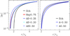 |
Fig. 1 Comparison of the temporal spacetime metric |𝑔tt|(= 1/|𝑔rr|) for different horizon radii: small (𝑔0 ≃ 1.5 rg, left panel) and standard (r0 = 2.0 rg, right panel). The black and blue curves represent the Schwarzschild metric and the RZ metric, with different parameters indicated by the model symbols (see Table 1). The red curve illustrates the Hayward metric with a parameter |

2.1.1 Inspection metric
To examine the dependence of the spacetime deviation on the different horizon radii, we introduced the inspection metrics A and AS. As the simplest representation, we focused on the parameters (a1 , ϵ) and set bi = 0 (that is, B2 = 1). The parameters and names of the physically motivated metrics and the inspection metric are summarized in Table 1, and the relationships of each metric are shown in Fig. 1. For the horizon radius r0 = 2rg, a larger (smaller) a1 results in a smaller (larger) magnitude of 𝑔tt compared to the Schwarzschild metric, corresponding to a shallower (deeper) gravitational potential (right panel of Fig. 1).
For the horizon radii r0 = 2.0 and 1.5, we introduced the ranges −0.50 ≤ a1 ≤ 0.50 and −0.25 ≤ a1 ≤ 0.50, respectively, within the constraints described in Cassing & Rezzolla (2023).
2.1.2 Hayward metric
The static black hole solution proposed by Hayward (Hayward 2006) replaces the singularity at r = 0 seen in the Schwarzschild black hole with a de Sitter center possessing a positive cosmological constant  :
:

where  is the Hubble length.
This model incorporates quantum corrections to address the singularity problem in standard black hole models, proposing a scenario where the central singularity is replaced with a regular finite-density core. This metric is particularly important in the study of nonsingular black holes, presenting a framework in which physical laws are maintained at the core. This metric is expected to be justified through phenomenological approaches, such as the equation of state for high-density matter and the upper limits of curvature, as well as in quantum gravity theories. It could deepen our understanding of black hole physics and provide new insights into quantum gravity effects at and beyond the event horizon. To investigate the maximum deviation of the Hayward solution from the Schwarzschild metric, we adopted an almost maximum value of  , which is close to the parameterized post-Newtonian limits and corresponds to a horizon radius of r0 ≃ 1.5 within the permissible range for the Sgr A* black hole solutions. This solution is described by the RZ metric with (ϵ, a1, a2, a3, a4) = (0.33333, −0.08333, −3.75000, 3.46667, −0.15897), as detailed in Kocherlakota & Rezzolla (2022).
We summarize the used metric in Table 1. Each metric has an apparent shadow radius rsh that is approximately within the 2σ range of the Sgr A* estimates (4.2 ≲ r/rg ≲ 5.6, Vagnozzi et al. 2023). Using the least squares method, the a1 value of the AS metric, which is closest to the physically motivated Hay0.75 metric, was found to be a1 ≃ −0.20 (see also Fig. 1). As a1 of the inspection metrics increases, both the photon radius rph and the shadow radius rsh monotonically increase.
2.2 GRMHD simulation setup
We focused our efforts on conducting two-dimensional GRMHD simulations using the RZ metric, employing the BHAC code (Porth et al. 2017; Olivares et al. 2019). Each simulation was conducted within a specified polar coordinate system, spanning 0.974 r0 ≤ r ≤ 2500 r𝑔 and 0 ≤ θ ≤ π. The grid spacing in the polar coordinates is logarithmic in the radial direction and uniform in the polar direction, with a total of (Nr, Nθ) = (512, 256) grid points. The consistency of the accretion flow is confirmed in Appendix A. As the initial condition for the GRMHD simulations, we introduced a hydrodynamic equilibrium torus (Font & Daigne 2002). The inner radius of the torus is set at rin = 20 r𝑔, with the density maximum located at rmax = 30 r𝑔. These measurements reference the horizon-penetrated RZ metric (e.g., Mizuno et al. 2018; Röder et al. 2023). The specific angular momentum of the initial torus ℓtorus is approximately 5.9. We utilized an ideal gas equation of state with an adiabatic index of  . To the stationary solution, we introduced a weak poloidal magnetic field, represented by a single loop and defined by the following vector potential:

The field strength was set such that  . To excite the magnetorotational instability inside the torus, the thermal pressure was perturbed by 4% white noise. To maintain the integrity of the fluid code and circumvent issues arising from vacuum regions, we instituted floor values for both the restmass density and the gas pressure, denoted as ρfl = 10−5r−3/2 and pfl = 10−7r−5/2, respectively. For all cells that meet the criterion ρ ≤ ρfl, we assigned a value of ρ = ρfl . Furthermore, should any cell satisfy p ≤ pfl, we set its value to p = pfl . Based on the metrics (Sect. 2.1) and initial conditions of the torus (Sect. 2.2), we performed the two-dimensional GRMHD simulations with BHAC to investigate the fundamental contribution of the metric deviation from the Schwarzschild spacetime.
2.3 GRRT simulation setup
The radiation properties and image morphology are calculated with the GRRT code employed in the BHOSS (Younsi et al. 2012, 2020), which solves the covariant radiative-transfer equation. In this paper we focus on two-dimensional GRMHD simulations during the quasi-stable accretion time window, assuming a uniform azimuthal distribution to perform GRRT simulations. The simulated movie is calculated at a frequency of 230 GHz, and the scaling of the mass accretion rate is set to be comparable to the mean total flux density of Sgr A* EHT observation on April 7, 2017 (~2.3 Jy; Event Horizon Telescope Collaboration 2022a). The black hole mass is set at 4.1 × 10⁶M⊙, and the distance is set at 8.1 kpc (Reid 2009; Reid et al. 2014, 2019). The calculation of the synthetic images is conducted using the fast-light approximation, wherein it is assumed that the fluid does not change during photon propagation, ensuring that each image corresponds to a single time slice. The image field of view is 400 µas, and the pixel resolution is 1 µas.
Synchrotron radiation is estimated to be the primary (and sole) source of emission at 230 GHz, with the electron energy distribution characterized by the “kappa” model (Xiao 2006) and a nonthermal energy contribution from the jet (Davelaar et al. 2019; Cruz-Osorio et al. 2022; Fromm et al. 2022; Moriyama et al. 2024; Zhang et al. 2024). The electron temperature is computed through the so-called two-temperature model so that the ion-to-electron temperature ratio is expressed as Ti /Te : = (Rlow + Rhighβ2)/(1 + β2) (Mócibrodzka et al. 2009). We focus on the single set of the parameters (Rlow, Rhigh, ϵκ) = (1, 160, 0.5), where ϵκ is the fraction of magnetic energy contributing to the heating of the radiating electrons introduced in the kappa-model (e.g., Cruz-Osorio et al. 2022). We introduced ϵκ for assessing the existence of the fainter jet component in the simulations focusing on Sgr A*. This value offers insight into realistic jet properties, amplifying the extended jet component (e.g., Fromm et al. 2022). In addition, we focused on an inclination angle of i = 30°, which is within the range of the EHT and GRAVITY constraints (Event Horizon Telescope Collaboration 2022e; GRAVITY Collaboration 2020).
3 GRMHD simulation results
Throughout the GRMHD simulations, we continuously monitored the mass accretion rate and the magnetic flux accreting across the horizon. Figure 2 shows the time evolution of the mass accretion rate (Ṁ), the magnetic flux (ϕBH), and the normalized magnetic flux  in code units for each spacetime:

where ρ is the mass density, ur is the radial component of the four-velocity of the fluid,  is the square root of the negative determinant of the metric, and Br is the radial component of the magnetic field. Both quantities are evaluated at the outer horizon r0. Our definition of the normalized magnetic flux Ψ differs by a factor of
  from the one defined in Tchekhovskoy et al. (2011). There is a rapid increase in Ṁ, ϕBH, and Ψ starting from t/tg = 1000, indicating intensified accretion onto the black hole. By t/tg = 13 500, the values of each reach a quasi-stable state. Hereafter, we focus on the phenomena during the quasi-stable phase where 13 500 ≤ t/tg ≤ 17 000 for all models.
In the quasi-equilibrium time range, the time-averaged values and standard deviations of Ṁ, ϕBH, and Ψ are presented in Table 2. The values of Ṁ, ϕBH, and Ψ in the quasi-stable time region for each spacetime are comparable. The values of Ψ in the AS and Hay0.75 metrics (6.95 ≤ Ψ ≤ 12.00) are slightly larger than those in the A metrics (5.40 ≤ Ψ ≤ 10.00). In conclusion, the mass accretion rate and the magnetic flux accreted across the horizon do not show a clear dependence on spacetime deviations from the Schwarzschild metric, although a decrease in the horizon size slightly increases the normalized magnetic flux.
The velocity field of the accretion flow near the black hole is highly sensitive to the underlying spacetime metric. In the GRMHD simulations, this dependence becomes evident when examining the distribution of velocities within the accretion flow. As shown in Fig. 3, the time-averaged distributions of the fluid’s three-velocity,  , where vi, and vi are the covariant and contravariant components of the accretion flow’s three-velocity; Porth et al. 2017), and the Alfvén velocity, vAlfvén, illustrate distinct behaviors influenced by the black hole’s metric. In every simulation executed, prominent outflow regions are observed both above and below the black hole, extending outward along the polar axis. These outflow regions are demarcated by a Bernoulli parameter Be > 1.02, indicating that material in these zones has sufficient energy to escape the black hole’s gravitational well.
The influence of the metric is particularly noticeable when examining the parameter a1, which affects the curvature of the black hole spacetime. For a1 ≥ 0, as a1 increases, stronger outflows, as more gravitational potential energy is released, resulting in higher values of both v and vAlfvén. This trend is consistent across most metrics, indicating a robust relationship between the metric’s curvature and the dynamics of the accretion flow. However, it is worth noting that for a1 = −0.25, the velocity field shows only minor deviations from that of a Schwarzschild black hole, suggesting that negative values of a1 may have less of an impact on the flow’s dynamics compared to positive values.
In addition to the changes in velocity, the region characterized by σB = 3 – a measure of plasma magnetization – also expands as a1 increases. This expansion indicates a growing influence of magnetic fields within the accretion flow, further influencing the dynamics near the black hole.
The outflows in each spacetime are not influenced by framedragging, preventing the formation of standard Blandford– Znajek-type jets (Blandford & Znajek 1977), although a relatively weak outflow region is still present (Fig. 3). To investigate the physical origin of the outflow, the radial velocity, and magnetization properties in each region are shown in Fig. 4. In this figure, the radially and time-averaged radial velocity, sgn , and the magnetization parameter, σB, in the range 100 ≤ r/rɡ ≤ 300, are plotted as functions of θ. The behaviors of the outflow region (gray region, where Be > 1.02), the disk region (40° ≲ θ ≲ 150°), and the polar region (θ ≲ 30° or θ ≳ 160°) are examined. Focusing on the top panels, the radial velocity in the disk region is nearly zero and shows no dependence on a1. In contrast, in the outflow region, the radial velocity is positive for all a1 values and increases monotonically with a1. This feature is consistent with the results shown in Fig. 3. Additionally, in simulations of Schwarzschild black holes and GRMHD spacetimes with a1 < 0, gas falls toward the black hole in the polar region. However, for a1 > 0, outflows are observed. This is because the gravitational potential for a1 > 0 is shallower compared to the Schwarzschild solution, allowing the interaction between axial flow and the outflow component to dominate over gravity. Focusing on the bottom panels, in all models, σB increases sharply at the boundary between the disk region and the outflow region, while the outflow region itself maintains relatively high magnetization parameters (σB = 1–5). This indicates that, in the simulations, magnetically driven outflows originate near the boundary between the disk region and the outflow region, driven by the magneto-centrifugal mechanism.
The same properties are observed in black hole metrics with small horizon sizes, as illustrated in Fig. 5. For instance, the Hayward metric, which exhibits curvature similar to the AS metric with a1 = −0.20, displays analogous features, confirming that both gravitational and magnetic effects play crucial roles in shaping the accretion dynamics in different spacetimes. The all outflow region has σB = 2–5 and driven by the magnetocentrifugal mechanism. These findings highlight the complex interplay between spacetime geometry, fluid dynamics, and magnetic fields in the vicinity of black holes.
Time-averaged mass accretion rate, magnetic flux, and normalized magnetic flux in GRMHD simulations across different spacetimes.
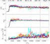 |
Fig. 2 Mass accretion rate (Ṁ), magnetic flux (ϕ), and normalized magnetic flux |

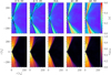 |
Fig. 3 Time-averaged distribution of the fluid and Alfvén velocities (|v| and vAlfvén). The dashed and solid black curves represent the boundary of the plasma magnetization, σB = 3 (σB = b2 /ρ, where b is the norm of the magnetic field in the fluid frame and ρ is the rest-mass density), and the Bernoulli parameter, Be = 1.02, respectively. |
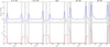 |
Fig. 4 Polar angle distribution of the radially and time-averaged radial velocity sgn |

4 GRRT simulation results
The different tendencies of the accretion flow in varying spacetimes result in systematic differences in the observed radiation. Figure 6 shows the light curve and power spectrum density for each A. Approximately 90% of the emission comes from r < 20 rg, while 50% of the emission originates from r < 6 rg.
The modulation index (σt(F)/〈F〉t, where 〈F〉t and σt(F) is the time-averaged and standard deviation of the light curve F) shown at the top of each panel indicates more intense fluctuations as a1 increases (σt(F)/〈F〉t = 1.2,1.4,1.4,1.9, and 2.3 for a1 = −0.5, −0.25,0.0,0.25, and 0.5). The power spectrum densities can be characterized by a power law profile with Pω ∝ ω−2.3±0.5 at the frequency of  . This property is broadly consistent with those produced by red noise (Pω ∝ ω−2) and previous research of the GRMHD simulations with/ without nonthermal particles (Georgiev et al. 2022; Moriyama et al. 2024).
The simulated images across different metrics exhibit a similar crescent-like structure, reflecting the spacetime structure of the emission region near the black hole. In the top panels of Fig. 7, we present the time-averaged images with different metric parameters a1 , while the bottom panel shows these same images convolved with the nominal EHT resolution of 20 µas, reflecting the expected observational limitations as a reference. Although we introduced the nonthermal contribution characterized by the kappa model, strong jet components are not detected in the simulations for each spacetime. As the metric parameter a1 increases, a subtle trend emerges: the size of the black hole’s shadow gradually decreases. The reduction in the shadow size aligns with the behavior of key radii, including the photon ring radius (rph) and the horizon radius (r0), as summarized in Table 1. Although the differences in image morphologies may appear visually subtle, we introduced the normalized cross-correlation, ρNX, to provide a quantitative measure of the structural differences across various images for each a1 value (e.g., Event Horizon Telescope Collaboration 2019b):
 (1)
(1)
where Ii and Ji represent the snapshot images for different models at each pixel labeled by i (1 ≤ i ≤ N), and ⟨I⟩ and σI denote the spatially averaged intensity and standard deviation, respectively. Each normalized cross-correlation in the figure is based on the time-averaged images of each metric case, compared to that of the Schwarzschild case. The images convolved at 20 µas (bottom panel) obscure minor differences other than size, with the corresponding ρNX(> 0.97) being comparable to the ρNX between the ground truth Schwarzschild and the 20 µas convolved images (= 0.97). These results suggest that detecting these differences in the averaged images with the current EHT resolution is challenging, as indicated by previous studies (Mizuno et al. 2018; Röder et al. 2023). We note slight differences in the normalized crosscorrelation between the time-averaged image and each snapshot, depending on the metric. Specifically, ρNX = (0.97 ± 0.02, 0.97 ± 0.016, 0.97 ± 0.02, 0.96 ± 0.02, 0.96 ± 0.02, 0.95 ± 0.03) for a1 = (−0.50, −0.25, 0.00, 0.25, 0.50), respectively. This feature also depends on variations in the azimuthal direction, indicating that future verification using three-dimensional GRMHD simulations is necessary.
Figure 8 summarizes the spacetime dependence of the modulation index. The modulation index increases with the growth of a1 for each metric (A and AS). The shadow size in the AS metric (4.42 ≤ rsh ≤ 4.95) is larger than that in the A metric (4.82 ≤ rsh ≤ 5.58), and the modulation index is also larger. These results indicate that as the event horizon and photon orbit decrease in size, the modulation index tends to increase. Furthermore, the characteristics of the Hayward metric align with this trend. The modulation index for a1 , estimated using the least squares method, and the metric Hay0.75 agree with the AS curve.
Because the gravitational potential of the Hayward metric for  is shallower than that of the Schwarzschild metric, and the horizon radius is smaller, the modulation index of the Hayward metric is expected to range from ~0.13 to 0.24, based on its dependence on the shadow size and a1. This range is larger than the modulation index of the 2017 Sgr A* light curves observed with the Atacama Large Millimeter/submillimeter Array (ALMA; 0.04–0.13; Wielgus et al. 2022), suggesting its potential to distinguish between physically motivated spacetimes. Based on these characteristics, we find a systematic correlation between luminosity fluctuations, characterized by the modulation index, and deviations in ɡtt from the Schwarzschild spacetime, as well as differences in horizon radii.
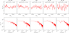 |
Fig. 6 Spacetime dependence of the 230 GHz light curves and power spectral densities. The panels, from left to right, correspond to black holes in A spacetimes with varying a1 parameters. |
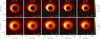 |
Fig. 7 Metric dependence of the time-averaged 230 GHz images (top panels) during the quasi-stable time window (13 500 ≤ t/tg ≤ 17 000). The bottom panels show images restored using a circular Gaussian beam with a full width at half maximum of 20 µas. The normalized cross-correlation, ρNX, between the Schwarzschild and each A metric is shown in the bottom-right corners. |
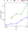 |
Fig. 8 Summary plot of the modulation index σt(F)/⟨F〉t. The corresponding a1 parameter of the plot of the Hayward metric is set to −0.2 based on the least squares method (see Sect. 2). |
5 Summary
In this paper we have introduced deviations from the Schwarzschild spacetime using the RZ-parameterized metric and investigated the behavior of accretion flows near the black hole through GRMHD and GRRT simulations. The deviations in each inspection spacetime are characterized by a1 on the order r−3, and the parameters were chosen such that the shadow size falls within the range of the Sgr A* observations from the 2017 EHT data. For a1 ≥ 0, as a1 increases, the gravitational potential becomes shallower compared to the Schwarzschild metric, and the characteristic radii of circular rotation decrease (Table 1). This spacetime results in the large dynamics of accretion flow and magnetic field characterized by the higher values of v and vAlfvén. These dynamic characteristics of the accretion flow are reflected in the observed radiation variations, with large luminosity fluctuations obtained for larger a1 values.
Another important aspect of the accretion model for Sgr A* is the behavior of relativistic jets. The existence of the jet in the Galactic Center has long been debated due to the lack of a clearly collimated outflow extending significant distances from the black hole.Nevertheless, certain cavity-like features and disordered yet bipolar structures have been proposed as indirect evidence of a weak jet (Royster et al. 2019; Yusef-Zadeh et al. 2020). Furthermore, several GRMHD models presented in Event Horizon Telescope Collaboration (2022e) suggest the presence of weak jet components (Chavez et al. 2024). The theory of jet power has a rich research history, often centered around the paradigm of black hole spin (e.g., Blandford & Znajek 1977; Tchekhovskoy et al. 2010) and variations or precession in the jet’s orientation (e.g., Steenbrugge & Blundell 2008; Steenbrugge et al. 2008, 2010). In Sect. 3 it is shown that the spacetime deviation from the Schwarzschild black hole can influence the strength of the magnetic field and fluid velocity in the outflow region (Fig. 3). However, this contribution is not sufficient to produce a clear difference in jet brightness in the GRRT simulation (Fig. 7).
The results of this research can be used to predict the magnitude of luminosity variations and the dynamics of accretion flows in black hole spacetime solutions with various physical motivations, which were not included in the simulations discussed here, by evaluating deviations from the Schwarzschild spacetime structure. The shallower gravitational potential, like the Hayward metric, compared with the Schwarzschild potential will provide higher fluid and Alfvén velocities, which in turn will provide the large radiation variation. Examples of black hole spacetimes with physical motivations include other regular black holes such as Hayward black holes, black holes in modified gravity theories, black holes with additional matter fields, black hole mimickers, exotic compact objects, and black holes with modifications from fundamental physics (see Olivares et al. 2020; Cruz-Osorio et al. 2021; Vagnozzi et al. 2023; Chatterjee et al. 2023b; Jiang et al. 2024).
The systematic dependence of accretion flow dynamics and flux variations on deviations from general relativity is expected to persist as more realistic simulation environments are introduced. To further advance this research and enable detailed comparisons between observational data and theoretical simulations, incorporating the azimuthal characteristics of accretion flows through three-dimensional GRMHD simulations and carefully accounting for nonthermal influences is essential (e.g., Meringolo et al. 2023; Imbrogno et al. 2024). Investigating luminosity variations within consistent torus models for Kerr black holes could provide valuable insights into whether these observational features are less dependent on specific accretion disk models (e.g., Cruz-Osorio et al. 2020; Lahiri et al. 2021; Gimeno-Soler et al. 2024; Uniyal et al. 2024). In addition to the above investigations, we plan to explore the effects of deviations in the ɡtϕ component, which characterizes the frame-dragging effect of a rotating black hole (e.g., Kocherlakota et al. 2023; Ma & Rezzolla 2024). The continued development of these simulations, combined with the comparison of statistical observational data on the variability of Sgr A*, has the possibility to contribute significantly to distinguishing between different black hole solutions.
Acknowledgements
We thank Prashant Kocherlakota for their insightful comments on this research. This research is supported by the European Research Council for the Advanced Grant “JETSET: Launching, propagation and emission of relativistic jets from binary mergers and across mass scales” (Grant No. 884631). ACO gratefully acknowledges “Ciencia Básica y de Frontera 2023–2024” program of the “Consejo Nacional de Humanidades, Ciencias y Tecnología” (CONAHCYT, México), projects CBF2023-2024-1102 and SNII 257435. YM is supported by the National Key R&D Program of China (grant no. 2023YFE0101200), the National Natural Science Foundation of China (grant no. 12273022), and the Shanghai Municipality Orientation Program of Basic Research for International Scientists (grant no. 22JC1410600). AU is supported by the Research Fund for Excellent International PhD Students (grant No. W2442004). The work at the IAA-CSIC is supported in part by the Spanish Ministerio de Economía y Competitividad (grants AYA2016- 80889-P, PID2019-108995GB-C21, PID2022-140888NB-C21), the Consejería de Economía, Conocimiento, Empresas y Universidad of the Junta de Andalucía (grant P18-FR-1769), the Consejo Superior de Investigaciones Científicas (grant 2019AEP112), and the State Agency for Research of the Spanish MCIU through the “Center of Excellence Severo Ochoa” grant CEX2021-001131-S funded by MCIN/AEI/ 10.13039/501100011033 awarded to the Instituto de Astrofísica de Andalucía.
Appendix A Confirmation test with a high-resolution GRMHD simulation
In this paper we have discussed in detail the behavior of accretion dynamics and the characteristics of luminosity variations in the spacetime near a black hole, based on specific simulation resolutions. To investigate the extent to which the dynamics of accretion flow depend on simulation resolution, we conducted simulations at multiple resolutions using the Schwarzschild metric. By systematically evaluating the effects of resolution on the dynamics and behavior of physical quantities, we aimed to confirm the robustness and reproducibility of the simulation methods. We performed GRMHD simulations under the same initial conditions with a high resolution of (Nr, Nθ) = (1024,512), where the radial and azimuthal directions were doubled in resolution. In this high-resolution simulation, it became possible to capture finer details of fluid motion and energy transport, and we examined how these results compared to those obtained with standard resolution, identifying any differences or consistencies. Figure A.1 shows the time-averaged spatial behavior of the fluid velocity distribution and Alfvén velocity. The simulation results at standard resolution discussed in the main text (Fig. 3) are consistent with those obtained in the high-resolution simulation, confirming that the dynamics of the accretion flow and the associated physical quantities exhibit similar behavior regardless of the differences in resolution. This result indicates that physical insights into the behavior of accretion flows and the dynamics of energy transport remain fundamentally unchanged even when the simulation resolution is increased. Thus, it is anticipated that the same approach will be effective in future high-resolution simulations and in analyzes that consider different spacetime geometries.
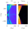 |
Fig. A.1 Same as Fig. 3 but based on the higher spatial resolution (Nr, Nθ) = (1024,512) compared with that in the main text (Nr, Nθ) = (512,256). |
Appendix B Light curve variation with a thermal electron distribution
In the main text, we focus on the radiating electron heating mechanism introduced in the kappa model (e.g., Cruz-Osorio et al. 2022) and investigates in detail the effects of spacetime deviation (a1) on accretion flow and luminosity variability. This approach serves as an initial step toward understanding how the electron heating mechanism influences radiation properties and their dependence on spacetime structure in the vicinity of black holes. Comprehensively understanding the possible range of modulation indices based on different electron heating mechanisms and initial magnetic field conditions is a key theme newly motivated by this study. Achieving this objective will require an extensive parameter survey, enabling a deeper exploration of various physical processes in black hole environments.
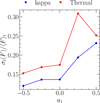 |
Fig. B.1 Modulation index σt(F)/⟨F〉t. with the inspection metric A based on the thermal (red) and kappa (blue) electron distribution. |
In this appendix we adopt a thermal Maxwellian distribution as an example of an alternative electron energy distribution. The modulation indices derived from this distribution are compared with those from the kappa model, with the results detailed in Fig. B.1. For this analysis, the spacetime structure of the black hole is modeled using the inspection metric A. Additionally, the scaling of the mass accretion rate is set, as in the main text, to match the average total flux density observed for Sgr A* by the EHT on April 7, 2017 (approximately 2.3 Jy). For a1 < 0 (a1 > 0), the modulation index is smaller (larger) compared to the Schwarzschild case, a trend consistent with the results obtained using the kappa model. Furthermore, when using the thermal model, radiation resulting from more complex accretion flow variability near the black hole tends to be more pronounced compared to the kappa model (e.g., Fromm et al. 2022). As a result, the modulation indices corresponding to each a1 are consistently larger for the thermal model than for the kappa model. Specifically, the modulation index for a1 = 0.25 (σt(F)/⟨F〉t = 0.3) is higher than both the value for a1 = 0.5 (0.25) and the kappa model value (0.23). The small variability observed in the 2017 Sgr A* ALMA light curve (0.04–0.13; Wielgus et al. 2022) suggests that the kappa model is preferable to the thermal model in spherically symmetric black hole spacetimes.
References
- Baganoff, F. K., Bautz, M. W., Brandt, W. N., et al. 2001, Nature, 413, 45 [Google Scholar]
- Blandford, R. D., & Znajek, R. L. 1977, MNRAS, 179, 433 [NASA ADS] [CrossRef] [Google Scholar]
- Cassing, M., & Rezzolla, L. 2023, MNRAS, 522, 2415 [NASA ADS] [CrossRef] [Google Scholar]
- Chael, A., Rowan, M., Narayan, R., Johnson, M., & Sironi, L. 2018, MNRAS, 478, 5209 [NASA ADS] [CrossRef] [Google Scholar]
- Chael, A., Lupsasca, A., Wong, G. N., & Quataert, E. 2023, ApJ, 958, 65 [NASA ADS] [CrossRef] [Google Scholar]
- Chan, C.-k., Psaltis, D., & Özel, F. 2013, ApJ, 777, 13 [NASA ADS] [CrossRef] [Google Scholar]
- Chan, H.-S., Chan, C.-k., Prather, B. S., Wong, G. N., & Gammie, C. 2024, ApJ, 964 [Google Scholar]
- Chatterjee, K., Younsi, Z., Liska, M., et al. 2020, MNRAS, 499, 362 [NASA ADS] [CrossRef] [Google Scholar]
- Chatterjee, K., Chael, A., Tiede, P., et al. 2023a, Galaxies, 11, 38 [NASA ADS] [CrossRef] [Google Scholar]
- Chatterjee, K., Younsi, Z., Kocherlakota, P., & Narayan, R. 2023b, arXiv e-prints [arXiv:2310.20043] [Google Scholar]
- Chavez, E., Issaoun, S., Johnson, M. D., et al. 2024, ApJ, 974, 116 [Google Scholar]
- Cruz-Osorio, A., Gimeno-Soler, S., & Font, J. A. 2020, MNRAS, 492, 5730 [NASA ADS] [CrossRef] [Google Scholar]
- Cruz-Osorio, A., Gimeno-Soler, S., Font, J. A., De Laurentis, M., & Mendoza, S. 2021, Phys. Rev. D, 103, 124009 [NASA ADS] [CrossRef] [Google Scholar]
- Cruz-Osorio, A., Fromm, C. M., Mizuno, Y., et al. 2022, Nat. Astron., 6, 103 [NASA ADS] [CrossRef] [Google Scholar]
- Davelaar, J., Olivares, H., Porth, O., et al. 2019, A&A, 632, A2 [NASA ADS] [CrossRef] [EDP Sciences] [Google Scholar]
- Do, T., Witzel, G., Gautam, A. K., et al. 2019, ApJ, 882, L27 [NASA ADS] [CrossRef] [Google Scholar]
- Dodds-Eden, K., Porquet, D., Trap, G., et al. 2009, ApJ, 698, 676 [NASA ADS] [CrossRef] [Google Scholar]
- Event Horizon Telescope Collaboration (Akiyama, K., et al.) 2019a, ApJ, 875, L1 [Google Scholar]
- Event Horizon Telescope Collaboration (Akiyama, K., et al.) 2019b, ApJ, 875, L4 [Google Scholar]
- Event Horizon Telescope Collaboration (Akiyama, K., et al.) 2022a, ApJ, 930, L12 [NASA ADS] [CrossRef] [Google Scholar]
- Event Horizon Telescope Collaboration (Akiyama, K., et al.) 2022b, ApJ, 930, L17 [NASA ADS] [CrossRef] [Google Scholar]
- Event Horizon Telescope Collaboration (Akiyama, K., et al.) 2022c, ApJ, 930, L14 [NASA ADS] [CrossRef] [Google Scholar]
- Event Horizon Telescope Collaboration (Akiyama, K., et al.) 2022d, ApJ, 930, L15 [NASA ADS] [CrossRef] [Google Scholar]
- Event Horizon Telescope Collaboration (Akiyama, K., et al.) 2022e, ApJ, 930, L16 [NASA ADS] [CrossRef] [Google Scholar]
- Font, J. A., & Daigne, F. 2002, MNRAS, 334, 383 [NASA ADS] [CrossRef] [Google Scholar]
- Fromm, C. M., Cruz-Osorio, A., Mizuno, Y., et al. 2022, A&A, 660, A107 [NASA ADS] [CrossRef] [EDP Sciences] [Google Scholar]
- Georgiev, B., Pesce, D. W., Broderick, A. E., et al. 2022, ApJ, 930, L20 [NASA ADS] [CrossRef] [Google Scholar]
- Gillessen, S., Eisenhauer, F., Trippe, S., et al. 2009, ApJ, 692, 1075 [NASA ADS] [CrossRef] [Google Scholar]
- Gimeno-Soler, S., Pimentel, O. M., Lora-Clavijo, F. D., Cruz-Osorio, A., & Font, J. A. 2024, Phys. Rev. D, 110, 023023 [Google Scholar]
- Gralla, S. E., Holz, D. E., & Wald, R. M. 2019, Phys. Rev. D, 100, 024018 [Google Scholar]
- GRAVITY Collaboration (Abuter, R., et al.) 2019, A&A, 625, L10 [NASA ADS] [CrossRef] [EDP Sciences] [Google Scholar]
- GRAVITY Collaboration (Jiménez-Rosales, A., et al.) 2020, A&A, 643, A56 [CrossRef] [EDP Sciences] [Google Scholar]
- Gurvits, L. I., Paragi, Z., Amils, R. I., et al. 2022, Acta Astronautica, 196, 314 [Google Scholar]
- Hayward, S. A. 2006, Phys. Rev. Lett., 96, 031103 [CrossRef] [PubMed] [Google Scholar]
- Himwich, E., Johnson, M. D., Lupsasca, A., & Strominger, A. 2020, Phys. Rev. D, 101, 084020 [NASA ADS] [CrossRef] [Google Scholar]
- Igumenshchev, I. V., Narayan, R., & Abramowicz, M. A. 2003, ApJ, 592, 1042 [Google Scholar]
- Imbrogno, M., Meringolo, C., Servidio, S., et al. 2024, ApJ, 972, L5 [Google Scholar]
- Jiang, H.-X., Dihingia, I. K., Liu, C., Mizuno, Y., & Zhu, T. 2024, J. Cosmology Astropart. Phys., 2024, 101 [Google Scholar]
- Johnson, M. D., Lupsasca, A., Strominger, A., et al. 2020, Sci. Adv., 6, eaaz1310 [Google Scholar]
- Kerr, R. P. 1963, Phys. Rev. Lett., 11, 237 [Google Scholar]
- Kocherlakota, P., & Rezzolla, L. 2022, MNRAS, 513, 1229 [NASA ADS] [CrossRef] [Google Scholar]
- Kocherlakota, P., Narayan, R., Chatterjee, K., Cruz-Osorio, A., & Mizuno, Y. 2023, ApJ, 956, L11 [NASA ADS] [CrossRef] [Google Scholar]
- Kocherlakota, P., Rezzolla, L., Roy, R., & Wielgus, M. 2024, Phys. Rev. D, 109, 064064 [NASA ADS] [CrossRef] [Google Scholar]
- Lahiri, S., Gimeno-Soler, S., Font, J. A., & Mejías, A. M. 2021, Phys. Rev. D, 103, 044034 [NASA ADS] [CrossRef] [Google Scholar]
- Liska, M., Hesp, C., Tchekhovskoy, A., et al. 2018, MNRAS, 474, L81 [Google Scholar]
- Ma, Y., & Rezzolla, L. 2024, Phys. Rev. D, 110, 024032 [Google Scholar]
- Marrone, D. P., Baganoff, F. K., Morris, M. R., et al. 2008, ApJ, 682, 373 [Google Scholar]
- McKinney, J. C., Tchekhovskoy, A., & Blandford, R. D. 2012, MNRAS, 423, 3083 [Google Scholar]
- Meringolo, C., Cruz-Osorio, A., Rezzolla, L., & Servidio, S. 2023, ApJ, 944, 122 [NASA ADS] [CrossRef] [Google Scholar]
- Mizuno, Y., Younsi, Z., Fromm, C. M., et al. 2018, Nat. Astron., 2, 585 [Google Scholar]
- Moriyama, K., Cruz-Osorio, A., Mizuno, Y., et al. 2024, ApJ, 960, 106 [NASA ADS] [CrossRef] [Google Scholar]
- Móscibrodzka, M., Gammie, C. F., Dolence, J. C., Shiokawa, H., & Leung, P. K. 2009, ApJ, 706, 497 [Google Scholar]
- Murchikova, L., White, C. J., & Ressler, S. M. 2022, ApJ, 932, L21 [NASA ADS] [CrossRef] [Google Scholar]
- Narayan, R., Igumenshchev, I. V., & Abramowicz, M. A. 2003, PASJ, 55, L69 [NASA ADS] [Google Scholar]
- Narayan, R., Sadowski, A., Penna, R. F., & Kulkarni, A. K. 2012, MNRAS, 426, 3241 [NASA ADS] [CrossRef] [Google Scholar]
- Neilsen, J., Nowak, M. A., Gammie, C., et al. 2013, ApJ, 774, 42 [NASA ADS] [CrossRef] [Google Scholar]
- Olivares, H., Porth, O., Davelaar, J., et al. 2019, A&A, 629, A61 [NASA ADS] [CrossRef] [EDP Sciences] [Google Scholar]
- Olivares, H., Younsi, Z., Fromm, C. M., et al. 2020, MNRAS, 497, 521 [Google Scholar]
- Övgün, A., Sese, L. J. F., & Pantig, R. C. 2024, Ann. Phys., 536, 2300390 [Google Scholar]
- Palumbo, D. C. M., & Wong, G. N. 2022, ApJ, 929, 49 [Google Scholar]
- Pantig, R. C., & Övgün, A. 2023, Ann. Phys., 448, 169197 [Google Scholar]
- Paul, D., Bhattacharjee, P., & Kalita, S. 2024, ApJ, 964, 127 [Google Scholar]
- Porth, O., Olivares, H., Mizuno, Y., et al. 2017, Computat. Astrophys. Cosmol., 4, 1 [NASA ADS] [CrossRef] [Google Scholar]
- Reid, M. J. 2009, Int. J. Mod. Phys. D, 18, 889 [NASA ADS] [CrossRef] [Google Scholar]
- Reid, M. J., Menten, K. M., Brunthaler, A., et al. 2014, ApJ, 783, 130 [Google Scholar]
- Reid, M. J., Menten, K. M., Brunthaler, A., et al. 2019, ApJ, 885, 131 [Google Scholar]
- Ressler, S. M., Quataert, E., & Stone, J. M. 2018, MNRAS, 478, 3544 [NASA ADS] [CrossRef] [Google Scholar]
- Ressler, S. M., Quataert, E., & Stone, J. M. 2020a, MNRAS, 492, 3272 [NASA ADS] [CrossRef] [Google Scholar]
- Ressler, S. M., White, C. J., Quataert, E., & Stone, J. M. 2020b, ApJ, 896, L6 [NASA ADS] [CrossRef] [Google Scholar]
- Rezzolla, L., & Zhidenko, A. 2014, Phys. Rev. D, 90, 084009 [Google Scholar]
- Röder, J., Cruz-Osorio, A., Fromm, C. M., et al. 2023, A&A, 671, A143 [NASA ADS] [CrossRef] [EDP Sciences] [Google Scholar]
- Royster, M. J., Yusef-Zadeh, F., Wardle, M., et al. 2019, ApJ, 872, 2 [Google Scholar]
- Sądowski, A., Narayan, R., Penna, R., & Zhu, Y. 2013, MNRAS, 436, 3856 [Google Scholar]
- Sengo, I., Cunha, P. V. P., Herdeiro, C. A. R., & Radu, E. 2023, J. Cosmology Astropart. Phys., 2023, 047 [Google Scholar]
- Steenbrugge, K. C., & Blundell, K. M. 2008, MNRAS, 388, 1457 [NASA ADS] [CrossRef] [Google Scholar]
- Steenbrugge, K. C., Heywood, I., & Blundell, K. M. 2008, MNRAS, 388, 1465 [CrossRef] [Google Scholar]
- Steenbrugge, K. C., Heywood, I., & Blundell, K. M. 2010, MNRAS, 401, 67 [NASA ADS] [CrossRef] [Google Scholar]
- Takahashi, R. 2004, ApJ, 611, 996 [Google Scholar]
- Takahashi, H. R., Ohsuga, K., Kawashima, T., & Sekiguchi, Y. 2016, ApJ, 826, 23 [Google Scholar]
- Tchekhovskoy, A., Narayan, R., & McKinney, J. C. 2010, ApJ, 711, 50 [NASA ADS] [CrossRef] [Google Scholar]
- Tchekhovskoy, A., Narayan, R., & McKinney, J. C. 2011, MNRAS, 418, L79 [NASA ADS] [CrossRef] [Google Scholar]
- Uniyal, A., Pantig, R. C., & Övgün, A. 2023, Phys. Dark Universe, 40, 101178 [Google Scholar]
- Uniyal, A., Dihingia, I. K., & Mizuno, Y. 2024, ApJ, 970, 172 [Google Scholar]
- Vagnozzi, S., Roy, R., Tsai, Y.-D., et al. 2023, Class. Quant. Grav., 40, 165007 [NASA ADS] [CrossRef] [Google Scholar]
- Walia, R. K., Ghosh, S. G., & Maharaj, S. D. 2022, ApJ, 939, 77 [Google Scholar]
- Wielgus, M., Marchili, N., Martí-Vidal, I., et al. 2022, ApJ, 930, L19 [NASA ADS] [CrossRef] [Google Scholar]
- Will, C. M. 2006, Liv. Rev. Relativ., 9, 3 [NASA ADS] [CrossRef] [Google Scholar]
- Xiao, F. 2006, Plasma Phys. Controlled Fusion, 48, 203 [NASA ADS] [CrossRef] [Google Scholar]
- Younsi, Z., Wu, K., & Fuerst, S. V. 2012, A&A, 545, A13 [NASA ADS] [CrossRef] [EDP Sciences] [Google Scholar]
- Younsi, Z., Zhidenko, A., Rezzolla, L., Konoplya, R., & Mizuno, Y. 2016, Phys. Rev. D, 94, 084025 [Google Scholar]
- Younsi, Z., Porth, O., Mizuno, Y., Fromm, C. M., & Olivares, H. 2020, in Perseus in Sicily: From Black Hole to Cluster Outskirts, 342, eds. K. Asada, E. de Gouveia Dal Pino, M. Giroletti, H. Nagai, & R. Nemmen, 9 [NASA ADS] [Google Scholar]
- Yusef-Zadeh, F., Bushouse, H., Wardle, M., et al. 2009, ApJ, 706, 348 [NASA ADS] [CrossRef] [Google Scholar]
- Yusef-Zadeh, F., Royster, M., Wardle, M., et al. 2020, MNRAS, 499, 3909 [NASA ADS] [CrossRef] [Google Scholar]
- Zhang, M., Mizuno, Y., Fromm, C. M., Younsi, Z., & Cruz-Osorio, A. 2024, A&A, 687, A88 [NASA ADS] [CrossRef] [EDP Sciences] [Google Scholar]
All Tables
Time-averaged mass accretion rate, magnetic flux, and normalized magnetic flux in GRMHD simulations across different spacetimes.
All Figures
|
Fig. 1 Comparison of the temporal spacetime metric |𝑔tt|(= 1/|𝑔rr|) for different horizon radii: small (𝑔0 ≃ 1.5 rg, left panel) and standard (r0 = 2.0 rg, right panel). The black and blue curves represent the Schwarzschild metric and the RZ metric, with different parameters indicated by the model symbols (see Table 1). The red curve illustrates the Hayward metric with a parameter |
| In the text | |
|
Fig. 2 Mass accretion rate (Ṁ), magnetic flux (ϕ), and normalized magnetic flux |
| In the text | |
|
Fig. 3 Time-averaged distribution of the fluid and Alfvén velocities (|v| and vAlfvén). The dashed and solid black curves represent the boundary of the plasma magnetization, σB = 3 (σB = b2 /ρ, where b is the norm of the magnetic field in the fluid frame and ρ is the rest-mass density), and the Bernoulli parameter, Be = 1.02, respectively. |
| In the text | |
|
Fig. 4 Polar angle distribution of the radially and time-averaged radial velocity sgn |
| In the text | |
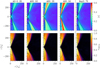 |
Fig. 5 Same as Fig. 3, but each profile is based on AS and Hay metrics. |
| In the text | |
|
Fig. 6 Spacetime dependence of the 230 GHz light curves and power spectral densities. The panels, from left to right, correspond to black holes in A spacetimes with varying a1 parameters. |
| In the text | |
|
Fig. 7 Metric dependence of the time-averaged 230 GHz images (top panels) during the quasi-stable time window (13 500 ≤ t/tg ≤ 17 000). The bottom panels show images restored using a circular Gaussian beam with a full width at half maximum of 20 µas. The normalized cross-correlation, ρNX, between the Schwarzschild and each A metric is shown in the bottom-right corners. |
| In the text | |
|
Fig. 8 Summary plot of the modulation index σt(F)/⟨F〉t. The corresponding a1 parameter of the plot of the Hayward metric is set to −0.2 based on the least squares method (see Sect. 2). |
| In the text | |
|
Fig. A.1 Same as Fig. 3 but based on the higher spatial resolution (Nr, Nθ) = (1024,512) compared with that in the main text (Nr, Nθ) = (512,256). |
| In the text | |
|
Fig. B.1 Modulation index σt(F)/⟨F〉t. with the inspection metric A based on the thermal (red) and kappa (blue) electron distribution. |
| In the text | |
Current usage metrics show cumulative count of Article Views (full-text article views including HTML views, PDF and ePub downloads, according to the available data) and Abstracts Views on Vision4Press platform.
Data correspond to usage on the plateform after 2015. The current usage metrics is available 48-96 hours after online publication and is updated daily on week days.
Initial download of the metrics may take a while.