| Issue |
A&A
Volume 696, April 2025
|
|
|---|---|---|
| Article Number | A36 | |
| Number of page(s) | 12 | |
| Section | Astrophysical processes | |
| DOI | https://doi.org/10.1051/0004-6361/202451577 | |
| Published online | 28 March 2025 | |
Flares from plasmoids and current sheets around Sgr A*
1
Department of Physics, University of Patras, Rio 26504, Greece
2
Research Center for Astronomy and Applied Mathematics, Academy of Athens, Athens 11527, Greece
3
Department of Physics, National and Kapodistrian University of Athens, University Campus Zografos, GR 15784, Athens, Greece
4
Institute of Accelerating Systems & Applications, University Campus Zografos, GR 15784, Athens, Greece
5
Institut für Theoretische Physik und Astrophysik, Universität Würzburg, Emil-Fischer-Strasse 31, 97074 Würzburg, Germany
6
Institut für Theoretische Physik, Goethe Universität Frankfurt, Max-von-Laue-Str.1, 60438 Frankfurt am Main, Germany
7
Max-Planck-Institut für Radioastronomie, Auf dem Hügel 69, D-53121 Bonn, Germany
⋆ Corresponding authors; This email address is being protected from spambots. You need JavaScript enabled to view it.
, This email address is being protected from spambots. You need JavaScript enabled to view it.
Received:
19
July
2024
Accepted:
24
February
2025
Abstract
Context. The supermassive black hole Sgr A* at the center of our galaxy produces repeating near-infrared flares that are observed by ground- and space-based instruments. This activity has been simulated in the past with magnetically arrested disk models that include stable jet formations. We used a different approach, considering a standard and normal evolution (SANE) multi-loop model that lacks a stable jet structure.
Aims. The main objective of this research is to identify regions that contain current sheets and high magnetic turbulence, and to subsequently generate a 2.2 μm light curve from nonthermal particles. These aims required the identification of areas that contain current sheets and high magnetic turbulence, and the averaging of the magnetization in the regions surrounding these areas. Subsequently, particle-in-cell fitting formulas were applied to determine the nonthermal particle distribution and to obtain the sought-after light curve. Additionally, we investigated the properties of the flares, in particular their evolution during flare events, and the similarity of flare characteristics between the generated and observed light curves.
Methods. We employed 2D general relativistic magnetohydrodynamic simulation data from a SANE multi-loop model and introduced thermal radiation to generate a 230 GHz light curve. Physical variables were calibrated to align with the 230 GHz observations. We identified current sheets by analyzing toroidal currents, magnetization, plasma β, density, and dimensionless temperatures. We studied the evolution of current sheets during flare events and calculated higher-energy nonthermal light curves, focusing on the 2.2 μm near-infrared range.
Results. We obtain promising 2.2 μm light curves whose flare duration and spectral index behavior align well with observations. Our findings support the association of flares with particle acceleration and nonthermal emission in current sheet plasmoid chains and at the boundary of the disk inside the funnel above and below the central black hole.
Key words: acceleration of particles / accretion / accretion disks / black hole physics / magnetic reconnection / magnetohydrodynamics (MHD) / radiation mechanisms: non-thermal
© The Authors 2025
 Open Access article, published by EDP Sciences, under the terms of the Creative Commons Attribution License (https://creativecommons.org/licenses/by/4.0), which permits unrestricted use, distribution, and reproduction in any medium, provided the original work is properly cited.
This article is published in open access under the Subscribe to Open model. This email address is being protected from spambots. You need JavaScript enabled to view it. to support open access publication.
1. Introduction
In the center of the Milky Way, at a distance of D ≃ 8.3 kpc, lies Sagittarius A* (Sgr A*), a 4.3 × 10⁶ M⊙ (GRAVITY Collaboration 2022) supermassive black hole. The accretion disk around it is optically thin, with collisionless, high-temperature, low-density plasma. Its bolometric luminosity is L ∼ 1036 erg s−1, which is in the sub-Eddington range (Genzel et al. 2010). The emission from Sgr A* is systematically monitored over a broad range of frequencies, allowing us to investigate the dynamics of the disk in the vicinity of a supermassive black hole.
Observations from the GRAVITY Collaboration have shown a hot spot rotating around Sgr A* with a period of ∼60 minutes at a distance of a few gravitational radii (hereafter rg) from the black hole (GRAVITY Collaboration 2018b). Sgr A* is known to exhibit variability in the near-infrared, which manifests itself in the form of several flares over a single day (Ghez et al. 2005b; Do et al. 2019). For the first time, GRAVITY observations revealed that a flare in Sgr A* coincided with a hot spot moving around the central black hole. Several investigations suggest that flares originate in highly magnetized structures that are formed in the innermost region of the black hole and produce synchrotron radiation (Dodds-Eden et al. 2009; Boehle et al. 2016; Ponti et al. 2017; Chatterjee et al. 2021; Scepi et al. 2022).
Analytical models have been applied to study the trajectory of the hot spots in the resulting light curve and show the importance of the effect of gravitational lensing (GRAVITY Collaboration 2005; Younsi & Wu 2015; Bauböck et al. 2020; Ball et al. 2021). As shown by Matsumoto et al. (2020), assuming that its motion is in the equatorial plane, the GRAVITY hot spot follows a circular path at super-Keplerian velocity. However, an outflowing conical sub-Keplerian orbit can fit these observations equally well (Antonopoulou & Nathanail 2024).
The theoretical astrophysics community has increasingly turned to numerical simulations, specifically general relativistic magnetohydrodynamic (GRMHD) simulations, in order to gain a comprehensive understanding of the dynamics involved in accreting black holes. Observations of flares and moving hot spots further emphasize the importance of considering both magnetic fields and fluid dynamics within the extreme gravitational environment near a black hole (Dexter et al. 2020; Porth et al. 2021; Chatterjee et al. 2021; Čemeljić et al. 2022; Scepi et al. 2022; Mellah et al. 2023; Lin & Yuan 2024).
Numerical investigations explore the formation of current sheets in the vicinity of a black hole and the subsequent production of plasmoids and plasmoid chains (Nathanail et al. 2020, 2022b; Ripperda et al. 2022). Current sheets are responsible for particle acceleration and the generation of variable nonthermal radiation. These models need to be supported by numerical studies of turbulence and magnetic reconnection in collisionless plasmas that self-consistently capture the dynamic interplay between particles and fields on kinetic plasma scales. Such investigations can be performed with particle-in-cell (PIC) simulations (Drake et al. 2012; Guo et al. 2014, 2015; Sironi & Spitkovsky 2014; Shay et al. 2014; Dahlin et al. 2014; Li et al. 2015, 2023; Petropoulou & Sironi 2018; Werner et al. 2018; Ball et al. 2018; Comisso & Sironi 2019). In particular, these investigations help us study the acceleration processes in detail by tracking individual particles, as well as characterize the properties of the particle distribution function, for example the shape of the distribution (power law or log-parabolic), the fraction of energy carried by nonthermal particles, the maximum particle energy, and others (e.g., Werner et al. 2018; Ball et al. 2018; Petropoulou et al. 2019; Zhang et al. 2023). Some of the particle properties, like the slope of the power-law distribution, can be related, through empirical expressions, to the local plasma properties, such as magnetization, σ ≔ B2/ρ (where B is the magnetic field strength and ρ is the density) and plasma β ≔ 2P/B2 (where P is the gas pressure). These prescriptions can then be combined with GRMHD simulations to anticipate the generation of nonthermal, high-energy electron distributions with properties that depend on the local physical conditions (Chatterjee et al. 2021; Scepi et al. 2022; Aimar et al. 2023; Lin et al. 2023; Mellah et al. 2023). The way to connect GRMHD simulations and PIC results is the following: After the plasma accretion process has reached an inflow equilibrium (Dexter et al. 2020), the thermal radiation is attributed to the hot electrons with a parameterized temperature derived from the simulation ion temperature (Mościbrodzka et al. 2016). To include nonthermal, radiating electrons, formulas from PIC simulations are employed. Nonthermal electron distributions are assumed in each cell, and they are assumed to depend on the magnetization (for σ < 5) and plasma β (Davelaar et al. 2019; Fromm et al. 2022; Cruz-Osorio et al. 2022). This study proposes a novel approach for incorporating nonthermal particles into simulation results: Current sheets are first identified (see also Vos et al. 2024), and then their environment is characterized in terms of averaged quantities of magnetization (σ) and plasma β. Finally, nonthermal particles are sourced from the plasma within the current sheet. In this study we utilized the 2D GRMHD simulations of Nathanail et al. (2020) to investigate the ability of the current sheet and plasmoids to produce the observed nonthermal flaring activity of Sgr A*. We applied a radiation model to produce light curves at 230 GHz (thermal radiation from the disk) and 2.2 μm (nonthermal radiation from current sheets; see also Scepi et al. 2022).
Section 2 describes the methodology of our investigation and is divided into three subsections: we introduce the GRMHD simulation setup (Sect. 2.1), the modeling of the radiation (Sect. 2.2), and the method with which we determined current sheets and their environment from the GRMHD simulation (Sect. 2.3). In Sect. 3 we present our results for the thermal (Sect. 3.1) and nonthermal radiation (Sect. 3.2). Finally, in Sect. 4 we present our conclusions and discuss prospects for future work.
2. Numerical setup
The numerical methods employed for the GRMHD simulation in this study closely mirror those used in previous research (Nathanail et al. 2020). We initialized the simulation with magnetic field configurations designed to generate multiple current sheets as the accretion system evolves. The formation of current sheets occurs in the vicinity of the black hole, and their subsequent reconnection gives rise to the development of multiple plasmoids and plasmoid chains. To assess the radiation characteristics of the current sheets formed and the subsequent generation of plasmoids, we employed a radiation proxy model. This model enables the calculation of thermal and nonthermal radiation at 230 GHz and 2.2 μm, respectively.
2.1. GRMHD simulation
The accretion disk surrounding a black hole can be conceptualized as a hydrodynamic system in the context of curved space-time, where the magnetic field significantly influences its dynamics. A GRMHD code integrates these physical properties into a unified numerical simulation and allows a robust evolution in time, where the accretion and accumulation of magnetic flux produce energetic phenomena. We employed the BHAC code (Porth et al. 2017), which solves the ideal magnetohydrodynamic equations in general relativity, namely
 (1)
(1)
 (2)
(2)
 (3)
(3)
where Tμν and *Fμν are the energy momentum tensor and the dual of the Faraday tensor, respectively. Here, we denote with ρ the rest-mass density and with uμ the fluid four-velocity. Some important characteristics of the code are the following: it implements second-order high-resolution shock-capturing finite-volume methods and adaptive mesh refinement wherever needed. It also implements constrained-transport (Del Zanna et al. 2007) to guarantee a divergence-free magnetic field (Olivares et al. 2019).
Furthermore, the model is axisymmetric (2D), and the coordinates of the initial torus-like plasma distribution are spherical (r × θ × ϕ). We used a logarithmic radial grid and the domain extends out to 2500 rg. The resolution of the model is 4096 × 2048 × 1 cells. The torus at the initial equilibrium state has constant specific angular momentum l = 4.28 (Fishbone & Moncrief 1976). The inner radius was set to rin = 6 rg and the pressure maximum radius to rmax = 12 rg. All quantities are calculated in geometrized units (G = c = 1) in which the gravitational radius is equal to rg = M. We considered a Kerr black hole with dimensionless spin a = J/M2 = 0.93, where J and M are the angular momentum and mass of the black hole, respectively. The radius of the event horizon is rh = 1.341 rg, and there are 29 × θres (θres = 2048 resolution in θ direction) grid cells inside the horizon.
The initial conditions for the magnetic field inside the torus consist of several loops of interchangeable clockwise–counterclockwise orientation between neighboring loops (see Fig. 1). To generate a magnetic field topology as described above, we used a vector potential, Aϕ:
 (4)
(4)
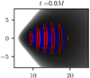 |
Fig. 1. Initial magnetic field (lines) and density (color) configuration in the initial torus. Axis coordinates are calculated in rg. Red and blue denote a clockwise and counterclockwise direction of the magnetic field. |
with
 (5)
(5)
![Mathematical equation: $$ \begin{aligned} B \equiv \cos {[(N-1)\theta ] \sin {[2\pi (r-r_{in})/\lambda _r]}}\ , \end{aligned} $$](/articles/aa/full_html/2025/04/aa51577-24/aa51577-24-eq6.gif) (6)
(6)
where N is the number of poloidal loops and λr their characteristic length scale, and ρmax is the maximum rest mass density of the disk.
State-of-the-art GRMHD codes have provided significant insights into the role of initialized magnetic fields with nested loops in jet formation (Narayan et al. 2022; Wong et al. 2021; Porth et al. 2019). The strength of the resulting jet is highly dependent on the initial conditions, particularly the size of the initial torus. A larger torus results in greater magnetic flux. For example, a standard and normal evolution (SANE) configuration with a small torus produces a weaker jet, while a magnetically arrested disk (MAD) configuration with a larger torus generates a more powerful jet.
In our case (SANE multi-loop), the initial setup causes the inverse polarity of the magnetic field to reconnect with the first polarity as the loops accrete. This prevents the black hole from accumulating sufficient magnetic flux to sustain a stable jet. We note that our simulations are based on a small torus configuration. For studies involving multi-loop and large torus setups, we refer readers to Jiang et al. (2023). It is important to note that the behavior is highly dependent on the initial conditions. To provide a physical basis for the initial multi-loop magnetic field, we refer to magnetorotational instability (MRI) simulations, which demonstrate a cycle of Bϕ changing polarity over time. This behavior is precisely what the initial multi-loop magnetic field aims to replicate (Nathanail et al. 2022a).
A key debate within the scientific community is whether the supermassive black hole at the center of our galaxy is capable of producing a stable jet. We have not yet observed a jet from Sgr A*, and it is an open question in which direction our models should go for the interpretation of phenomena near the black hole. As discussed in Nathanail et al. (2022a), images at 43 and 86 GHz will produce an extended stable jet base in the case of the MAD model, whereas in the case of the SANE multi-loop model, the images will possibly have an extended jet-like structure only in the flaring state. We expect that new images of the Sgr A* black hole will further clarify the landscape of pertinent models.
Furthermore, it is important to emphasize that while 2D GRMHD simulations are valuable for exploring the dynamics of accretion flows and jet formation, they inherently impose certain limitations compared to 3D simulations. In 2D, the axisymmetric assumption restricts the development of non-axisymmetric instabilities, such as the MRI turbulence, which plays a crucial role in angular momentum transport and magnetic field amplification. This simplification can lead to an over-simplified representation of the physical processes within the accretion disk and jet, potentially underestimating or misrepresenting phenomena like turbulent magnetic field structures and dynamo effects. Additionally, 2D simulations cannot fully capture the three-dimensional nature of jet collimation, twisting, and asymmetries caused by disk-jet interactions. As a result, while 2D models offer computational efficiency and valuable insights, they may not accurately represent the complexity and richness of the physics inherent to astrophysical systems, underscoring the importance of 3D simulations for comprehensive studies.
2.2. Radiation model
In this subsection we discuss and present in detail the model that we used for the thermal and nonthermal radiation expected from plasma in the accretion flow. We employed an approximate “proxy” model for radiation that integrates the thermal emissivity across the entire disk. The validity of this method has been tested in the past against general relativistic radiative transfer (GRRT) calculations (Porth et al. 2019). These comparisons demonstrated a close correspondence between the proxy method’s results, the detailed GRRT calculations, and the observed variability in the light curve. Scepi et al. (2022) employed a similar strategy to investigate flares originating from current sheets and plasmoids for MAD models.
The total luminosity Lν emitted by the fluid at a specific frequency ν (in units of ergs per second per Hz), is calculated based on the following equation:
 (7)
(7)
where jν is the emissivity of thermal or nonthermal processes at a specific frequency1 and τν is the opacity of the fluid to a given process at frequency ν. The terms  represents the infinitesimal volume element dV for each grid point. Close to the black hole radiation in specific is suppressed by the gravitational redshift term (gredshift3; Viergutz 1993), where
  . Here, A = (r2 + a2)2 − a2Δsin2θ, Σ = r2 + a2cos2θ and Δ = r2 − 2rM + a2. The parameter a corresponds to the spin of the black hole, while M represents its mass, which is fixed at 1 in these forms (an estimation of gredshift for r = 2rg, θ = π/4 and a = 0.93 is approximately on the order of 10−1). The observable radiation flux is given by Fν = Lν/4πD2, where the distance from the black hole is D = 8.277 kpc (GRAVITY Collaboration 2022). The integration of the luminosity works best when the viewing angle is nearly face on, as we are not taking the effects of Doppler beaming and gravitational lensing into account. The difference of such a method compared with a full GRRT calculation is of order of unity (Scepi et al. 2022).
At 230 GHz, the thermal electron synchrotron radiation comes predominantly from the disk region, namely π/3 ≲ θ ≲ 2π/3. To calculate the synchrotron emission of a thermal distribution of plasma, we utilized the formula developed by Leung et al. (2011, see also Pandya et al. 2016). At 230 GHz, the emissivity of a fluid element in the disk is given by the equation
 (8)
(8)
Here ne is the electron number density and X ≡ ν/νs, where νs ≡ (2/9)νLΘe2sin λ (λ is the particle pitch angle with respect to the direction of the magnetic field), and νL ≡ eB/(2πmec) is the Larmor frequency. The dimensionless proton temperature Θp, is defined as Θp = kβTp/(mpc2), where kβ is the Boltzmann constant and Tp is the proton temperature. This then calculated from the GRMHD simulation as Θp = P/ρ (Porth et al. 2017). We use Θe to denote the dimensionless temperature of the electrons, defined as Θe = kβTe/(mec2). Using the above relations, the formula is transformed to
 (9)
(9)
where mp and me are the masses of the proton and electron, respectively. It is important to mention that the composition of the fluid was assumed to be electron-proton plasma. The ratio Tp/Te was calculated from the prescription of Mościbrodzka et al. (2016), which describes the electron-to-proton coupling in low (disk) and high magnetized regions (funnel), namely
 (10)
(10)
where Rhigh and Rlow are free parameters that determine the heating ratio of electrons. In our calculations we set Rhigh = 20 and Rlow = 1, since we did not focus on a large parametric investigation of flares from such configurations. In Dihingia et al. (2023a) and Dihingia et al. (2023b), was made a comparison between two-temperature GRMHD model with cooling or no cooling effect and various prescriptions of temperature ratios proposed by various studies (Mościbrodzka et al. 2016; Dihingia et al. 2023a; Meringolo et al. 2023). Some results suggest that, within the disk region, the model proposed by Mościbrodzka et al. (2016) provides a closer approximation to the GRMHD two-temperature cooling model compared to other prescriptions. The electron temperature in a GRMHD simulation can be determined through two temperature simulations that independently evolve this quantity (Jiang et al. 2023). Such studies highlight the importance of self-consistently evolving the electron temperature to accurately explore the thermal synchrotron radiation (Jiang et al. 2024).
The thermal radiation absorption term e−τν is important only inside the disk. The optical depth is defined as τν = ∫π/3θ0aν, thds where  (π/3 ≤ θ0 ≤ 2π/3 are the latitudinal limits of the disk). In the case of local thermal equilibrium, the source function of the emitting material is given by the Planck function Bν. Then, the absorption coefficient of the material can be expressed as
 (11)
(11)
where
![Mathematical equation: $$ \begin{aligned} B_{\nu }=(2h\nu ^3/c^2)[\exp (h\nu /kT_e)-1]^{-1} \end{aligned} $$](/articles/aa/full_html/2025/04/aa51577-24/aa51577-24-eq15.gif) (12)
(12)
is the Planck function. So, the total luminosity for thermal radiation at each grid point (r0, θ0) is calculated as follows: First, we determined the emissivity at the point. Next, we computed the absorption term at all grid points (r, θ), where r = r0 and π/3 ≤ θ ≤ θ0. The sum of absorption coefficients (aν, th) at these points provides us with the value of the optical depth τν at (r0, θ0). In this way, it is like integrating along light rays perpendicular to the equatorial plane.
The nonthermal emissivity at 2.2 μm, which is attributed to the synchrotron radiation of relativistic electrons, is given by (Rybicki & Lightman 1986; Ghisellini 2013)
 (13)
(13)
where UB = B2/(8π) is the energy density of the magnetic field. One needs also to determine the nonthermal electron distribution n(γ) = Kγ−p, so K is the electron number density multiplied by the efficiency ϵ of the radiation mechanism, and p is the slope of the distribution.
In the case of nonthermal radiation the integration of Eq. (7) is performed along the radial direction. In the funnel region (see, e.g., the colored region in Fig. 3), this is like integrating along rays perpendicular to the equatorial plane. The optical depth in this case is τν = ∫rrmaxaν, nthds, where  . aν, nth is the dimensionless absorptivity; for the nonthermal process, it is defined as
 (14)
(14)
(Ghisellini 2013; Pandya et al. 2016), where the function fa(p) is a product of Γ functions, approximated as
 (15)
(15)
also in this case, the total luminosity for nonthermal radiation at each grid point is calculated as follows: First, we determined the emissivity at the point (r0, θ0). Next, we computed the absorption term at all grid points (r, θ), where r0 ≤ r ≤ rmax and θ = θ0. The sum of absorption coefficients (aν, nth) at these points provides us with the value of the optical depth, τν, at (r0, θ0).
A GRMHD simulation does not have the necessary micro-physics to follow the acceleration of particles and extract the electron distribution function or the efficiency for microscopic processes occurring within the plasma. To incorporate how energy is transferred from the magnetic field to the plasma, we used two different post-processing formulas from results of PIC simulations. The first approach is from a local investigation of idealized current sheets (Ball et al. 2018). The second one is from an investigation of microphysical properties of special-relativistic turbulence (Meringolo et al. 2023). The first approach was applied to the current sheets in the funnel region above the disk boundary, and the second one in the vicinity of the disk boundary. The results of such local investigations give us the opportunity to approximate the properties of the accelerated particles that will eventually radiate through the local plasma characteristics. We first defined the nonthermal acceleration efficiency, ϵ, as the fraction of the kinetic energy carried by the nonthermal particles to the kinetic energy of the total electron population,
![Mathematical equation: $$ \begin{aligned} \epsilon =\frac{\int _{\gamma _{pc}}^{\infty }(\gamma -1)[\frac{\mathrm{d}N}{\mathrm{d}\gamma }-f_{MB}(\gamma ,\Theta _e)]\mathrm{d}\gamma }{\int _{\gamma _{pc}}^{\inf }(\gamma -1)\frac{\mathrm{d}N}{\mathrm{d}\gamma }\mathrm{d}\gamma }\ , \end{aligned} $$](/articles/aa/full_html/2025/04/aa51577-24/aa51577-24-eq20.gif) (16)
(16)
where γpc denotes the peak of the spectrum and fMB is a relativistic Maxwellian fitting function.
According to Ball et al. (2018), Eq. (17) gives us the slope of the spectrum with respect to the magnetization, σ, and plasma β:
 (17)
(17)
where  , Bp = 3.7σ−0.19, and Cp = 23.4σ0.26. Moreover, the electron nonthermal efficiency with respect to the magnetization (σ) and plasma β is
 (18)
(18)
where Aϵ = 1 − 1/(4.2σ0.55 + 1), Bϵ = 0.64σ0.07, and Cϵ = −68σ0.13. On the other hand, Eq. (19) approximates the slope, p (for Eq. (19) it holds that p = k − 1) with respect to the same parameters based on Meringolo et al. (2023):
 (19)
(19)
where k0 = 2.8, k1 = 0.2, k2 = 1.6, and k3 = 2.25. The efficiency of particle acceleration in turbulent plasmas is equal to
![Mathematical equation: $$ \begin{aligned} \epsilon = e_0 + \frac{e_1}{\sqrt{\sigma }}+e_2\sigma ^{0.1}\tanh [e_3\beta \sigma ^{0.1}]\ , \end{aligned} $$](/articles/aa/full_html/2025/04/aa51577-24/aa51577-24-eq25.gif) (20)
(20)
where e0 = 1, e1 = −0.23, e2 = 0.5 and e3 = −10.18.
In Sect. 2.3 we elaborate on how we determined current sheets and their associated parameters, such as the magnetization and plasma β, in their vicinity. The reason we are interested in the latter is because dissipative current sheets are fed with plasma from their environment. These conditions determine the strength of the nonideal electric fields that accelerate particles and the rate of energy dissipation. All empirical relations that describe properties of the accelerated particle populations refer to the σ and plasma β parameters in the upstream regions of the current sheets. Once these areas of interest are identified, these formulas can then be applied to determine the slope of the distribution of accelerated electrons within the current sheets or turbulent regions at the disk boundary.
2.3. Determination of current sheets and their environment
The PIC simulations that investigate current sheets start with a specific magnetization, a specific plasma β and an initial current layer in the middle. As the magnetic field evolves magnetic reconnection events take place, magnetic energy is dissipated, and particles are accelerated from the thermal pool to higher energies. Equations (17) and (19) are fitting models of the results of such PIC simulations and give us the slope of the spectrum of the nonthermal electrons as functions of GRMHD quantities. It is important to emphasize that the parameter values that must be used in these formulas are roughly those set as initial conditions in a PIC simulation. As it turns out, these values are maintained during the calculation only in the environment surrounding the current sheets.
So, in order to use Eqs. (17) and (19), it is necessary to constrain the current sheet and its surrounding environment. First, it is useful to distinguish the regions where current sheets form from the polarity reversal of the magnetic fields (Fig. 2, reversal of Bz). We utilized five variables to determine the current sheets, which are as follows: toroidal current Jϕ := (∇×B)ϕ, density ρ, magnetization σ, plasma β and dimensionless temperature Θp (normalized to mc2, which is equal to P/ρ). The remaining plots in Fig. 2 provide limits for each parameter that defines the exact region where a current sheet occurs. As we see in Fig. 2, a current sheet is characterized by high values of toroidal current, high values of density, low values of magnetization, high values of plasma β and high values of dimensionless temperature. Thus, we set the following limits for each parameter: |Jϕ|> 10−4, a density floor (cutoff) at ρcut = 2 × 10⁻⁵, a magnetization ceiling cutoff at σcut = 10, a plasma β floor at βcut = 10−3 and finally a temperature floor at Θp = 10−3. By combining these constraints, we obtained the red regions in Fig. 3, which are clearly associated with the current sheets we identified. Additionally, the plasma in these red-colored regions has undergone the reconnection process. Efficient particle acceleration occurs in regions with high magnetization and low plasma β (Ball et al. 2018). Such regions develop only in the funnel region, so we applied the above methodology exclusively to the plasma within this region.
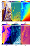 |
Fig. 2. Upper panel (from left to right): Magnetic field Bz component, toroidal current, and density. Lower panel (from left to right): Magnetization, plasma β, and dimensionless temperature Θp. By setting limits on these parameters, we define the red regions in Fig. 3. |
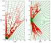 |
Fig. 3. Determination of plasma (red) in the reconnection region and places of high magnetic turbulence. They are selected after applying limits on the toroidal current, magnetization, plasma β, density, and dimensionless temperature. The green grid corresponds to the discretization for the purpose of parameter averaging. The snapshot is the same as that shown in Fig. 2. |
Following this procedure, we identified the current sheets developed in the simulation. The next step involved characterizing the current sheet environment in terms of averaged quantities in order to be able to use Eqs. (17) and (19) to determine the plasma within the current sheet. To achieve this, a discretization method was employed, wherein the region was divided into cells with a radial length of 1 rg and a meridional extent of 10 degrees in the θ direction. In each cell that contains part of a current sheet (red region), we calculated the mean values of magnetization, σ, and plasma β, of their environment (white region) over two cells to the right and two to the left in the θ direction, namely
 (21)
(21)
 (22)
(22)
Subsequently, the slope of the nonthermal electrons inside the current sheet or in the turbulent plasma in each cell is computed using Eqs. (17) and (19) with parameters values as  and
and  . The plasma assumed to be accelerated corresponds to the region depicted in red in Fig. 3.
3. Results
In the next two subsections, we present our results on the thermal and nonthermal radiation. The first part covers calculations at 230 GHz (thermal component), which help calibrate the physical parameters for Sgr A*. Further calculations provide information about the model’s variability compared to observations. Subsequently, we present results from the nonthermal radiation calculations at 2.2 μm, including the resulting light curve, an analysis of flares, and a comparison with the GRMHD simulation results.
3.1. Radiation at 230 GHz
Observations of Sgr A* at 230 GHz have been conducted by various telescopes, including the Submillimeter Array (SMA), the Atacama Large Millimeter/submillimeter Array (ALMA), and notably, the Event Horizon Telescope (EHT). The EHT in particular has provided a wealth of high-resolution images from the innermost region of the accretion disk onto Sgr A* itself, presenting an invaluable resource for the scientific community (EHT Collaboration 2022a,b,c,d,e,f). Thus, there exists a plethora of data on the properties of the light curve at that particular frequency. Therefore, utilizing much of these data, our main goals are to reproduce the main features of the light curve at 230 GHz (amplitude and variability) by calibrating the various physical parameters from dimensionless code units to actual physical units. When we combine how the flux changes with distance and angle (as illustrated in Fig. 4), it becomes clear that the majority of the radiation is emanating from a distance of approximately 10 rg. This underscores that the events we are studying occur in extremely close proximity to the black hole, and consequently, the critical data points we are interested in are highly concentrated in this area.
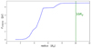 |
Fig. 4. Cumulative 230 GHz flux from all angles θ for radii less than or equal to r. |
As we know from observations (Wielgus et al. 2022), the radiation flux of Sgr A* at 230 GHz is approximately stable. To turn the parameters of the GRMHD simulation from code units to physical cgs units, a conversion and calibration of variables is necessary. We defined a scaling parameter (S) that appropriately multiplies physical quantities such as the magnetic field (B), pressure (P), and density (ρ) to convert values of physical quantities from geometric (code) units to cgs units. Obviously, the conversion leaves dimensionless quantities such as Θe, σ, and β unchanged:
 (23)
(23)
 (24)
(24)
 (25)
(25)
Through an iterative procedure applied in various snapshots of the GRMHD calculation, the model limited the radiation flux in a range around 4 Jy and finally produced the value of the scaling parameter S. After calculating the parameter S, we could calculate the radiation flux at all snapshots and finally produce the light curve at 230 GHz. The upper panel of Fig. 5 presents the light curve at 230 GHz (red line). Noticeably, the radiation flux remains almost constant throughout the calculation period. The higher flux values observed in the beginning of the light curve gradually decrease toward the end of the evolution.
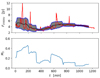 |
Fig. 5. Top panel: Simulated light curve at 230 GHz (red line), the moving average of the simulated light curve (m3, in a time window of 3 hours; black line), and the 1s3 standard deviation (gray area). Lower panel: Measure of the variability of the simulated light curve (M3), defined as M3 = s3/m3. |
To investigate the variability of the light curve, we defined the moving average radiation flux over a 3-hour period (m3, black line in Fig. 5) and the standard deviation over the same duration (s3, gray area in Fig. 5). The lower panel of Fig. 5 shows the spread of M3 where M3 = s3/m3. M3 is a measure of the variability of the light curve and can be compared with historical observations from Sgr A* (Fig. 6).
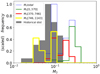 |
Fig. 6. Distribution of the M3 of the simulated light curve at 230 GHz (blue) compared with historical data from observations of Sgr A* (gray). We have divided the simulated light curve and its respective M3 into three time intervals: t ∈ [0, 370] min (green), t ∈ [370, 746] min (red), and t ∈ [746, 1143] min (yellow). |
The Sgr A* light curve shifts and changes over time due to a combination of stellar winds and turbulence on various scales. Longer changes come from variations in the stellar winds, especially near the S stars. Shorter changes happen because of turbulence closer to the center. The spread of M3 in Fig. 5 exhibits a downward trend, suggesting that if we keep running the same simulation for further time, the flare variability will eventually stabilize at lower levels. Figure 6 is a histogram of M3 that provides a broader view derived from observing Sgr A* (see Wielgus et al. 2022); the other distributions are derived from the simulation results for different time windows. Our model appears to align well with the observations. As previously mentioned, our GRMHD simulation corresponds to the SANE configuration (SANE multi-loop). According to the EHT publication (EHT Collaboration 2022e), these models demonstrate better consistency with the variability constraints compared to MAD models. It is important to keep in mind about Fig. 6 that the yellow line distribution represents the last part of the M3 curve inside the time interval t ∈ [746, 1143] min. This closely aligns with the observations and shows that a new calculation of the same model for longer times will probably yield the desired variability in the light curve. However, for a more accurate study of variability, it would be necessary to incorporate phenomena such as Doppler beaming and lensing effects into the calculations. These aspects were deliberately excluded, as their inclusion would deviate from the primary objective of this work.
3.2. Results at 2.2 μm (near-infrared flares)
3.2.1. Light curve and statistics
In Fig. 3 we carefully mark the specific areas where nonthermal radiation processes occur. These dynamic areas reside within the funnel region and in the limit of the disk. There is an environment characterized by high magnetization and low plasma (β) values, which are needed to activate the radiation mechanisms with sufficient efficiency. In Sect. 2.3 we discuss in detail that it is this local environment that characterizes the process of acceleration for the plasma residing within current sheets.
Using data from these regions, we calculated the light curve at 2.2 μm, and our results are depicted in Fig. 7. Notably, during quiescent states, the average flux is remarkably low, consistent with observations. Within the simulation, several flares occur, each typically exceeding a flux of > 1.5 mJy (Witzel et al. 2021; von Fellenberg et al. 2023). Noteworthy is that fact that there are four flares during the simulation time that surpass this threshold, with an additional three flares marginally meeting the criteria for acceptance as flares. One particularly significant radiation flare, with a flux of approximately 7 mJy and a longer duration than typical flares, stands out as a potential candidate within the observed limits for both flux and duration, resembling the unprecedented flare reported in Do et al. (2019).
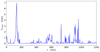 |
Fig. 7. Simulated light curve at 2.2 μm. Our model can produce one very bright flare of around 7 mJy and another three that pass the 1.5 mJy threshold. |
In a theoretical comparison with observations, we do not have a flux limit that allows us to define what is considered a flare and what not, but it is obvious that the values of the flux in Fig. 7 increase by several orders of magnitude between a quiescent and a flare state (F ≳ 1.5 mJy). Sgr A* produces flares with lower flux but also some very bright ones (F > 6 mJy; Do et al. 2019) like those produced in our model. In Fig. 8 we see a comparison of the historical flux distribution in histogram for Sgr A* from Witzel et al. (2018) as presented in Do et al. (2019) compared to the high flux flare observed in 2019. The probability of observing such a flare (> 6 mJy) was computed to be less than 0.05% (Witzel et al. 2018). Our model is capable of reproducing high-flux flares that cover the full range of observations.
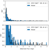 |
Fig. 8. Histogram comparing our model with observations from Do et al. (2019). The lower panel is a zoomed-in view. |
According to Fig. 8 our model appears to have fairly good statistics in terms of the population of flares. This is not the case for Sgr A* flares generated from MAD models, which seem to show a very large population of flares and tend to overproduce the quiescent state flux (Dexter et al. 2020; Scepi et al. 2022; White & Quataert 2022). This is probably due to the very strong magnetic field they possess, and the fact that the main source of the flares is the current sheet in the equator, which feeds high values of absorptivity in the density due to the ̇M (as seen characteristically in the paper of Scepi et al. 2022).
It is important to remark that in our method for computing the light curve, we have not taken the effect of cooling into account. For reference, we estimated the cooling time of a particle with The Lorentz factor, γ, due to synchrotron radiation was calculated as
 (26)
(26)
where the Lorentz factor, γ, is γ = (ν/νL)1/2. Using typical values for magnetic field B from our model, approximately 60 G for the region of interest calculating the cooling time from relation (26) we obtain tsyn ∼ 3 min. In future research, cooling should be examined more thoroughly, as it can influence the light curve results at near-infrared and higher wavelengths.
3.2.2. Properties of flares
In the upper panel of Fig. 9 we zoom in on the first major flare within the time range t ∈ [86, 150], hereafter referred to as Flare A. In the lower panel, we zoom in on a second, smaller flare within the time range t ∈ [879, 926], hereafter referred to as Flare B. We examined how the properties of each flare change across three different stages: the pre-flare state, which occurs when the flux is several orders of magnitude smaller than 1 mJy; the dim state, which occurs when the flux begins to increase (as shown in Fig. 11, where the spectral index also increases) and finally, the bright state, which occurs when the flux exceeds 1 mJy. In both flares, we can see the specific points and their corresponding colors that represent the three different states. Each point is derived from a specific snapshot of the GRMHD simulation. The first flare is characterized by a distinct peak, while the second flare has two peaks. Similar phenomena have been observed (GRAVITY Collaboration 2018a). The classification of points into the different flare states was based on flux and spectral index. The rationale for this classification is clearly illustrated in Fig. 11.
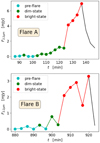 |
Fig. 9. Part of the light curve at 2.2 μm. Top: Flare A during the period t ∈ [86, 150] min (the first bright flare with approximately 7 mJy radiation flux). Bottom: Flare B during the period t ∈ [879, 926] min (a bright flare with two peaks). The duration of the flares is about 40–60 minutes. We divided the light curve into three states: pre-flare, dim state, and bright state. This separation is based on the flux and spectral index |
Following the same calculation methods used for the nonthermal radiation, we estimated the radiation flux at three additional frequencies: 6.66, 7.95, and 18.1 GHz, which correspond to the M, L, and H bands, respectively. The primary frequency of our calculation, 2.2 μm, corresponds to the K band for Sgr A*. For this calculation we used two snapshots at times t = 136 min and t = 920 min, one for each flare at the peak of the bright state. We thus extracted the spectrum of our model for this flare state (Fig. 10). The fitting curves in Fig. 10 can give us the spectral index (which is defined as the exponent of a power-law-like F ∝ νa) for each flare. The two values that we obtained (a = −0.46 and a = −0.44) are within the observed range (Ghez et al. 2005a,b; Bremer et al. 2011).
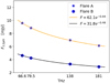 |
Fig. 10. Radiation flux around 2.2 μm for the frequencies 66.6 (M band), 79.5 (L band), 138 (K band), and 181 THz (H band) for Flare A (stars) and Flare B (circles). The fitting lines (black and orange) correspond to power laws where the exponential gives us the spectral index of the spectrum, in our case a = −0.44 for Flare A and a = −0.46 for Flare B. |
During a flare, the flux and the spectral index increase simultaneously. We categorized the points into three groups, distinguished by the colors used to represent them. Figure 11 shows the evolution of the spectral index as the flares transition from the pre-flare state to the dim state and finally to the bright state. The fitting power-law curve (orange line) approximates how the spectral index evolves as the flare transitions from one state to the next, which is comparable to observations (Bremer et al. 2011). The same colors were used to distinguish the points in Fig. 9.
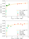 |
Fig. 11. Spectral index vs. flux for Flare A (top) and Flare B (bottom). The dots correspond to the snapshots that are marked in Fig. 9: the pre-flare (cyan), dim (green), and bright states (red) of each flare. The orange lines are a fitting power-law curve, which can be compared with observations. |
3.2.3. Flare states compared with the GRMHD simulation
We wanted to see how the peaks in the light curve relate to the GRMHD calculation from which the phenomena originated. Therefore, we plotted the parameters ρ, σ, and plasma β, which play crucial roles in shaping the current sheet (Fig. 12). The plots refer to the three states of the second flare we investigated, specifically the snapshots at times t = 886 min (pre-flare), t = 900 min (dim state), and t = 910 min (bright state). The corresponding points of these snapshots can be seen in the light curve of Fig. 9.
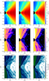 |
Fig. 12. Top row: Density of Flare B (t ∈ [886, 963] min) in its three states: pre-flare, dim state, and bright state, at snapshots t = 886 min, t = 900 min, and t = 910 min, respectively. Middle row: Magnetization (σ) at the same snapshots. Bottom row: Plasma β at the same snapshots. |
The plot of the density (ρ; top row in Fig. 12) shows a clear structure in the upper funnel region that appears as the flare transitions from one state to the next. This structure is also characterized by low magnetization and high plasma β. According to the definition given above, it constitutes a clear current sheet that, in the bright state, is surrounded by regions with high values of magnetization (σ; middle row in Fig. 12) and low plasma β (bottom row in Fig. 12). These are ideal conditions for radiating nonthermal radiation. This current sheet in the bright state can be characterized as a plasmoid chain, similar to those seen in localized PIC simulations (Ball et al. 2018; Sironi & Spitkovsky 2014; Petropoulou & Sironi 2018).
It is important to emphasize that this increase in magnetization, σ, and decrease in plasma β in the bright state of the flares (conditions ideal for the activation of flares) are also found at the boundaries of the disk. These are possible regions for flare generation through high magnetic turbulence in the plasma, as mentioned in Sect. 2.2. Figure 12 clearly shows that the creation of the current sheet inside the funnel region is a phenomenon perfectly connected to the organization of the magnetic field and results in the creation of conditions (magnetization and plasma β) that will activate nonthermal particles in the current sheet itself and along the disk boundary.
Indeed, the areas that radiate are the current sheet and the disk boundary as shown in Fig. 13. Figure 13 illustrates the radiation flux (in mJy), the slope p and the efficiency ϵ at time t = 910 min (the bright state of Flare B that we investigated). The visible boxes in each plot correspond to the identification of current sheets and their environment as shown in Fig. 3. Within each box, all plasma quantities are averaged in order to characterize this specific reconnection region. However, only the plasma within the current sheet layer – determined by the constraints and limits discussed in Sect. 2.3 – is considered to have the specific slope and efficiency, producing the reported flux. Two-thirds of the nonthermal radiation flux comes from the disk boundary, where the turbulent plasma dominates, while one-third comes from the current sheet.
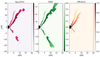 |
Fig. 13. Radiation flux at 2.2 microns (in mJy), slope (p), and efficiency (ϵ) in each grid point of the GRMHD simulation shown in the left, middle, and right panels, respectively, for the bright state of Flare B. |
Similar phenomena can be observed in Flare A at time t = 136 min. A clear current sheet has produced a plasmoid chain, and the local environment is characterized by high magnetization and low plasma β (see Fig. 15). Accordingly, the slope p and the efficiency ϵ (middle and right panel of Fig. 14) peak at the current sheet and produce the radiation flux (left panel of Fig. 14), which strengthens our conclusions about how the flares are generated in this particular calculation.
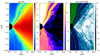 |
Fig. 15. Density (left panel), magnetization, σ (middle panel) and plasma β (right panel) of Flare A in the bright state. |
4. Conclusions
We have analyzed data from the GRMHD simulation of Nathanail et al. (2020), specifically focusing on model D, which is characterized as a SANE multi-loop model. Unlike MAD simulations, this model describes the accretion disk of a black hole without the production of a stable jet.
Applying a thermal radiation model to this particular simulation enabled us to reproduce the light curve at 230 GHz, from which we were able to calibrate the simulation variables. Encouragingly, the model’s variability demonstrated good agreement with observations, prompting us to conduct larger simulations with extended time evolution.
To calculate the nonthermal radiation from the simulation, we introduced a novel method that identifies current sheets and places with high magnetic turbulence. This identification, based on the magnetic field polarity reversals, is done by constraining primarily the current density together with the micro-physical plasma parameters, such as magnetization and plasma β. After the identification, all quantities are averaged in the local environment. The constraints we placed on the parameters provided clear spatial boundaries within which to apply the model that calculates the nonthermal radiation. This association both advances our comprehension of the fundamental processes at play and provides a crucial framework for future investigations in similar contexts.
The results for the light curve at 2.2 μm are very encouraging as they produce both small flares up to 2 mJy and a couple of brighter ones that reach 7 mJy. The duration of such flares is also consistent with observations. Further analysis of the flare spectral index verified the success of the model in reproducing the observations. It is interesting that, during the evolution of the flare, the spectrum follows a power law similar to those given by the observations with spectral index a = −0.44.
In summary, we emphasize once again that a very important result of this work is the identification of the source of flaring nonthermal radiation in GRMHD simulations. We have shown that such flares most likely originate from current sheets and their associated plasmoid chains in the funnel region, as well as from the disk boundary due to magnetic turbulence.
5. Data availability
The data underlying this article will be shared upon reasonable request to the corresponding author (URL source: Zenodo Record
There seems to be some confusion in the literature in the definition of “emissivity”. Emissivity usually expresses the effectiveness of the surface of a material in emitting energy as thermal radiation. In the recent astrophysical literature, however, emissivity jν is defined as the energy loss per unit time per frequency per unit volume (e.g., Leung et al. 2011; Ghisellini 2013; Scepi et al. 2022). Note that Rybicki & Lightman (1986) define jν as the “emission coefficient”, i.e., the energy loss per unit time per frequency per unit volume per steradian.
Acknowledgments
ID is supported by the Hellenic Foundation for Research and Innovation (HFRI) under the 4th Call for HFRI PhD Fellowships (Fellowship Number: 9239). Support comes from the ERC Advanced Grant “JETSET: Launching, propagation and emission of relativistic jets from binary mergers and across mass scales” (Grant No. 884631). This work was supported by computational time granted from the National Infrastructures for Research and Technology S.A. (GRNET S.A.) in the National HPC facility – ARIS. Simulations were performed also on the GOETHE-HLR cluster at CSC in Frankfurt).
References
- Aimar, N., Dmytriiev, A., Vincent, F. H., et al. 2023, A&A, 672, A62 [NASA ADS] [CrossRef] [EDP Sciences] [Google Scholar]
- Antonopoulou, E., & Nathanail, A. 2024, A&A, 690, A240 [NASA ADS] [CrossRef] [EDP Sciences] [Google Scholar]
- Ball, D., Sironi, L., & Özel, F. 2018, ApJ, 862, 80 [Google Scholar]
- Ball, D., Özel, F., Christian, P., Chan, C.-K., & Psaltis, D. 2021, ApJ, 917, 8 [NASA ADS] [CrossRef] [Google Scholar]
- Bauböck, M., Dexter, J., Abuter, R., et al. 2020, A&A, 635, A143 [CrossRef] [EDP Sciences] [Google Scholar]
- Boehle, A., Ghez, A., Schödel, R., et al. 2016, ApJ, 830, 17 [NASA ADS] [Google Scholar]
- Bremer, M., Witzel, G., Eckart, A., et al. 2011, A&A, 532, A26 [NASA ADS] [CrossRef] [EDP Sciences] [Google Scholar]
- Čemeljić, M., Yang, H., Yuan, F., & Shang, H. 2022, ApJ, 933, 55 [CrossRef] [Google Scholar]
- Chatterjee, K., Markoff, S., Neilsen, J., et al. 2021, MNRAS, 507, 5281 [NASA ADS] [CrossRef] [Google Scholar]
- Comisso, L., & Sironi, L. 2019, ApJ, 886, 122 [Google Scholar]
- Cruz-Osorio, A., Fromm, C. M., Mizuno, Y., et al. 2022, Nat. Astron., 6, 103 [NASA ADS] [CrossRef] [Google Scholar]
- Dahlin, J., Drake, J., & Swisdak, M. 2014, Phys. Plasmas, 21, 092304 [NASA ADS] [Google Scholar]
- Davelaar, J., Olivares, H., Porth, O., et al. 2019, A&A, 632, A2 [NASA ADS] [CrossRef] [EDP Sciences] [Google Scholar]
- Del Zanna, L., Zanotti, O., Bucciantini, N., & Londrillo, P. 2007, A&A, 473, 11 [NASA ADS] [CrossRef] [EDP Sciences] [Google Scholar]
- Dexter, J., Tchekhovskoy, A., Jiménez-Rosales, A., et al. 2020, MNRAS, 497, 4999 [Google Scholar]
- Dihingia, I. K., Mizuno, Y., Fromm, C. M., & Rezzolla, L. 2023a, MNRAS, 518, 405 [NASA ADS] [Google Scholar]
- Dihingia, I. K., Mizuno, Y., Fromm, C. M., & Younsi, Z. 2023b, ArXiv e-prints [arXiv:2305.09698] [Google Scholar]
- Do, T., Witzel, G., Gautam, A. K., et al. 2019, ApJ, 882, L27 [NASA ADS] [CrossRef] [Google Scholar]
- Dodds-Eden, K., Porquet, D., Trap, G., et al. 2009, ApJ, 698, 676 [NASA ADS] [CrossRef] [Google Scholar]
- Drake, J., Swisdak, M., & Fermo, R. 2012, ApJ, 763, L5 [NASA ADS] [Google Scholar]
- EHT Collaboration 2022a, ApJ, 930, L12 [NASA ADS] [CrossRef] [Google Scholar]
- EHT Collaboration 2022b, ApJ, 930, L13 [NASA ADS] [CrossRef] [Google Scholar]
- EHT Collaboration 2022c, ApJ, 930, L14 [NASA ADS] [CrossRef] [Google Scholar]
- EHT Collaboration 2022d, ApJ, 930, L15 [NASA ADS] [CrossRef] [Google Scholar]
- EHT Collaboration 2022e, ApJ, 930, L16 [NASA ADS] [CrossRef] [Google Scholar]
- EHT Collaboration 2022f, ApJ, 930, L17 [NASA ADS] [CrossRef] [Google Scholar]
- Fishbone, L. G., & Moncrief, V. 1976, ApJ, 207, 962 [NASA ADS] [CrossRef] [Google Scholar]
- Fromm, C. M., Cruz-Osorio, A., Mizuno, Y., et al. 2022, A&A, 660, A107 [NASA ADS] [CrossRef] [EDP Sciences] [Google Scholar]
- Genzel, R., Eisenhauer, F., & Gillessen, S. 2010, Rev. Mod. Phys., 82, 3121 [Google Scholar]
- Ghez, A., Salim, S., Hornstein, S. D., et al. 2005a, ApJ, 620, 744 [NASA ADS] [CrossRef] [Google Scholar]
- Ghez, A., Hornstein, S., Lu, J., et al. 2005b, ApJ, 635, 1087 [NASA ADS] [Google Scholar]
- Ghisellini, G. 2013, Radiative processes in high energy astrophysics (Springer), 873 [Google Scholar]
- GRAVITY Collaboration (Broderick, A. E., et al.) 2005, MNRAS, 363, 353 [NASA ADS] [CrossRef] [Google Scholar]
- GRAVITY Collaboration (Abuter, R., et al.) 2018a, A&A, 618, L10 [NASA ADS] [CrossRef] [EDP Sciences] [Google Scholar]
- GRAVITY Collaboration (Abuter, R., et al.) 2018b, A&A, 615, L15 [NASA ADS] [CrossRef] [EDP Sciences] [Google Scholar]
- GRAVITY Collaboration (Abuter, R., et al.) 2022, A&A, 657, L12 [NASA ADS] [CrossRef] [Google Scholar]
- Guo, F., Li, H., Daughton, W., & Liu, Y.-H. 2014, Phys. Rev. Lett., 113, 155005 [Google Scholar]
- Guo, F., Liu, Y.-H., Daughton, W., & Li, H. 2015, ApJ, 806, 167 [NASA ADS] [CrossRef] [Google Scholar]
- Jiang, H.-X., Mizuno, Y., Fromm, C. M., & Nathanail, A. 2023, MNRAS, 522, 2307 [NASA ADS] [CrossRef] [Google Scholar]
- Jiang, H.-X., Mizuno, Y., Dihingia, I. K., et al. 2024, A&A, 688, A82 [NASA ADS] [CrossRef] [EDP Sciences] [Google Scholar]
- Leung, P. K., Gammie, C. F., & Noble, S. C. 2011, ApJ, 737, 21 [NASA ADS] [CrossRef] [Google Scholar]
- Li, X., Guo, F., Li, H., & Li, G. 2015, ApJ, 811, L24 [NASA ADS] [Google Scholar]
- Li, X., Guo, F., Liu, Y.-H., & Li, H. 2023, ApJ, 954, L37 [NASA ADS] [Google Scholar]
- Lin, X., & Yuan, F. 2024, ArXiv e-prints [arXiv:2405.17408] [Google Scholar]
- Lin, X., Li, Y.-P., & Yuan, F. 2023, MNRAS, 520, 1271 [NASA ADS] [CrossRef] [Google Scholar]
- Matsumoto, T., Chan, C.-H., & Piran, T. 2020, MNRAS, 497, 2385 [NASA ADS] [CrossRef] [Google Scholar]
- Mellah, I. E., Cerutti, B., & Crinquand, B. 2023, A&A, 677, A67 [NASA ADS] [CrossRef] [EDP Sciences] [Google Scholar]
- Meringolo, C., Cruz-Osorio, A., Rezzolla, L., & Servidio, S. 2023, ApJ, 944, 122 [NASA ADS] [CrossRef] [Google Scholar]
- Mościbrodzka, M., Falcke, H., & Shiokawa, H. 2016, A&A, 586, A38 [Google Scholar]
- Narayan, R., Chael, A., Chatterjee, K., Ricarte, A., & Curd, B. 2022, MNRAS, 511, 3795 [NASA ADS] [CrossRef] [Google Scholar]
- Nathanail, A., Fromm, C. M., Porth, O., et al. 2020, MNRAS, 495, 1549 [Google Scholar]
- Nathanail, A., Dhang, P., & Fromm, C. M. 2022a, MNRAS, 513, 5204 [NASA ADS] [CrossRef] [Google Scholar]
- Nathanail, A., Mpisketzis, V., Porth, O., Fromm, C. M., & Rezzolla, L. 2022b, MNRAS, 513, 4267 [NASA ADS] [CrossRef] [Google Scholar]
- Olivares, H., Porth, O., Davelaar, J., et al. 2019, A&A, 629, A61 [NASA ADS] [CrossRef] [EDP Sciences] [Google Scholar]
- Pandya, A., Zhang, Z., Chandra, M., & Gammie, C. F. 2016, ApJ, 822, 34 [Google Scholar]
- Petropoulou, M., & Sironi, L. 2018, MNRAS, 481, 5687 [NASA ADS] [CrossRef] [Google Scholar]
- Petropoulou, M., Sironi, L., Spitkovsky, A., & Giannios, D. 2019, ApJ, 880, 37 [Google Scholar]
- Ponti, G., George, E., Scaringi, S., et al. 2017, MNRAS, 468, 2447 [NASA ADS] [CrossRef] [Google Scholar]
- Porth, O., Olivares, H., Mizuno, Y., et al. 2017, Comput. Astrophys. Cosmol., 4, 1 [Google Scholar]
- Porth, O., Chatterjee, K., Narayan, R., et al. 2019, ApJS, 243, 26 [Google Scholar]
- Porth, O., Mizuno, Y., Younsi, Z., & Fromm, C. 2021, MNRAS, 502, 2023 [NASA ADS] [CrossRef] [Google Scholar]
- Ripperda, B., Liska, M., Chatterjee, K., et al. 2022, ApJ, 924, L32 [NASA ADS] [CrossRef] [Google Scholar]
- Rybicki, G. B., & Lightman, A. P. 1986, Radiative Processes in Astrophysics (Wiley-VCH) [Google Scholar]
- Scepi, N., Dexter, J., & Begelman, M. C. 2022, MNRAS, 511, 3536 [NASA ADS] [CrossRef] [Google Scholar]
- Shay, M., Haggerty, C., Phan, T., et al. 2014, Phys. Plasmas, 21, 19 [Google Scholar]
- Sironi, L., & Spitkovsky, A. 2014, ApJ, 783, L21 [NASA ADS] [CrossRef] [Google Scholar]
- Viergutz, S. 1993, A&A, 272, 355 [NASA ADS] [Google Scholar]
- von Fellenberg, S. D., Witzel, G., Bauböck, M., et al. 2023, A&A, 669, L17 [NASA ADS] [CrossRef] [EDP Sciences] [Google Scholar]
- Vos, J. T., Olivares, H., Cerutti, B., & Mościbrodzka, M. 2024, MNRAS, submitted [arXiv:2309.03267] [Google Scholar]
- Werner, G. R., Uzdensky, D. A., Begelman, M. C., Cerutti, B., & Nalewajko, K. 2018, MNRAS, 473, 4840 [Google Scholar]
- White, C. J., & Quataert, E. 2022, ApJ, 926, 136 [NASA ADS] [Google Scholar]
- Wielgus, M., Marchili, N., Martí-Vidal, I., et al. 2022, ApJ, 930, L19 [NASA ADS] [CrossRef] [Google Scholar]
- Witzel, G., Martinez, G., Hora, J., et al. 2018, ApJ, 863, 15 [NASA ADS] [CrossRef] [Google Scholar]
- Witzel, G., Martinez, G., Willner, S. P., et al. 2021, ApJ, 917, 73 [NASA ADS] [CrossRef] [Google Scholar]
- Wong, G. N., Du, Y., Prather, B. S., & Gammie, C. F. 2021, ApJ, 914, 55 [NASA ADS] [CrossRef] [Google Scholar]
- Younsi, Z., & Wu, K. 2015, MNRAS, 454, 3283 [NASA ADS] [CrossRef] [Google Scholar]
- Zhang, H., Sironi, L., Giannios, D., & Petropoulou, M. 2023, ApJ, 956, L36 [NASA ADS] [CrossRef] [Google Scholar]
All Figures
|
Fig. 1. Initial magnetic field (lines) and density (color) configuration in the initial torus. Axis coordinates are calculated in rg. Red and blue denote a clockwise and counterclockwise direction of the magnetic field. |
| In the text | |
|
Fig. 2. Upper panel (from left to right): Magnetic field Bz component, toroidal current, and density. Lower panel (from left to right): Magnetization, plasma β, and dimensionless temperature Θp. By setting limits on these parameters, we define the red regions in Fig. 3. |
| In the text | |
|
Fig. 3. Determination of plasma (red) in the reconnection region and places of high magnetic turbulence. They are selected after applying limits on the toroidal current, magnetization, plasma β, density, and dimensionless temperature. The green grid corresponds to the discretization for the purpose of parameter averaging. The snapshot is the same as that shown in Fig. 2. |
| In the text | |
|
Fig. 4. Cumulative 230 GHz flux from all angles θ for radii less than or equal to r. |
| In the text | |
|
Fig. 5. Top panel: Simulated light curve at 230 GHz (red line), the moving average of the simulated light curve (m3, in a time window of 3 hours; black line), and the 1s3 standard deviation (gray area). Lower panel: Measure of the variability of the simulated light curve (M3), defined as M3 = s3/m3. |
| In the text | |
|
Fig. 6. Distribution of the M3 of the simulated light curve at 230 GHz (blue) compared with historical data from observations of Sgr A* (gray). We have divided the simulated light curve and its respective M3 into three time intervals: t ∈ [0, 370] min (green), t ∈ [370, 746] min (red), and t ∈ [746, 1143] min (yellow). |
| In the text | |
|
Fig. 7. Simulated light curve at 2.2 μm. Our model can produce one very bright flare of around 7 mJy and another three that pass the 1.5 mJy threshold. |
| In the text | |
|
Fig. 8. Histogram comparing our model with observations from Do et al. (2019). The lower panel is a zoomed-in view. |
| In the text | |
|
Fig. 9. Part of the light curve at 2.2 μm. Top: Flare A during the period t ∈ [86, 150] min (the first bright flare with approximately 7 mJy radiation flux). Bottom: Flare B during the period t ∈ [879, 926] min (a bright flare with two peaks). The duration of the flares is about 40–60 minutes. We divided the light curve into three states: pre-flare, dim state, and bright state. This separation is based on the flux and spectral index |
| In the text | |
|
Fig. 10. Radiation flux around 2.2 μm for the frequencies 66.6 (M band), 79.5 (L band), 138 (K band), and 181 THz (H band) for Flare A (stars) and Flare B (circles). The fitting lines (black and orange) correspond to power laws where the exponential gives us the spectral index of the spectrum, in our case a = −0.44 for Flare A and a = −0.46 for Flare B. |
| In the text | |
|
Fig. 11. Spectral index vs. flux for Flare A (top) and Flare B (bottom). The dots correspond to the snapshots that are marked in Fig. 9: the pre-flare (cyan), dim (green), and bright states (red) of each flare. The orange lines are a fitting power-law curve, which can be compared with observations. |
| In the text | |
|
Fig. 12. Top row: Density of Flare B (t ∈ [886, 963] min) in its three states: pre-flare, dim state, and bright state, at snapshots t = 886 min, t = 900 min, and t = 910 min, respectively. Middle row: Magnetization (σ) at the same snapshots. Bottom row: Plasma β at the same snapshots. |
| In the text | |
|
Fig. 13. Radiation flux at 2.2 microns (in mJy), slope (p), and efficiency (ϵ) in each grid point of the GRMHD simulation shown in the left, middle, and right panels, respectively, for the bright state of Flare B. |
| In the text | |
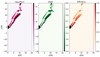 |
Fig. 14. Same as Fig. 13 but for the bright state of Flare A. |
| In the text | |
|
Fig. 15. Density (left panel), magnetization, σ (middle panel) and plasma β (right panel) of Flare A in the bright state. |
| In the text | |
Current usage metrics show cumulative count of Article Views (full-text article views including HTML views, PDF and ePub downloads, according to the available data) and Abstracts Views on Vision4Press platform.
Data correspond to usage on the plateform after 2015. The current usage metrics is available 48-96 hours after online publication and is updated daily on week days.
Initial download of the metrics may take a while.