| Issue |
A&A
Volume 691, November 2024
|
|
|---|---|---|
| Article Number | A309 | |
| Number of page(s) | 17 | |
| Section | The Sun and the Heliosphere | |
| DOI | https://doi.org/10.1051/0004-6361/202449396 | |
| Published online | 21 November 2024 | |
Different manifestations of a loop-like transient brightening in solar atmospheres
1
Institute of Space Physics, Luoyang Normal University, Luoyang 471934, PR China
2
Yunnan Key Laboratory of the Solar physics and Space Science, Kunming 650216, PR China
3
Henan Key Laboratory of Electromagnetic Transformation and Detection, Luoyang Normal University, Luoyang 471934, PR China
4
Research Center for Novel Solar-Blind Ultraviolet and Infrared Photoelectronic Detectors of Henan province, Luoyang 471934, PR China
5
Key Laboratory of Solar Activity and Space Weather, National Space Science Center, Chinese Academy of Sciences, Beijing 100190, PR China
6
Yunnan Observatories, Chinese Academy of Sciences, Kunming 650216, PR China
⋆ Corresponding author; fenghq9921@163.com
Received:
30
January
2024
Accepted:
6
October
2024
Context. Small-scale transient brightenings that are the consequence of magnetic reconnection play pivotal roles in the heating process of solar atmospheres. These phenomena contain key information about the dynamic evolution of the solar magnetic field. The fine-scale structures triggered by instabilities in these brightenings are intimately connected with the release of magnetic energy.
Aims. To better understand the conversion and release of magnetic energy in small-scale heating events, we investigated the thermal-dynamical behaviors of a loop-like transient brightening (LTB) with plasma blobs.
Methods. We used the spectroscopic and slit-jaw imaging observations taken from the Interface Region Imaging Spectrograph and the extreme-ultraviolet images taken from the Atmospheric Imaging Assembly on board the Solar Dynamics Observatory to analyze the plasma properties of an LTB that occurred on February 28, 2014. The space-time maps were created to present the spatial evolution of the LTB, and the light curves were calculated to illustrate the heating process. Additionally, we employed the differential emission measure (DEM) method to compute the temperature and emission measure of the LTB. In order to investigate the plasma motion along the line-of-sight direction, a double-Gaussian function was used to fit the Si IV spectral profiles.
Results. The spectrum and DEM analysis indicate that the LTB was constituted by multithermal plasma with temperatures reaching up to 5.4 × 10⁶ K. The space-time maps of the emission and the Gaussian-fitting results of the Si IV line demonstrate that the LTB not only exhibited bidirectional flows, but was also twisted. Several plasma blobs were identified in the spine of the LTB, suggesting the potential presence of a tearing-mode instability. The low-temperature bands peaked approximately one minute prior to the high-temperature bands, suggesting the occurrence of a heating process driven by magnetic reconnection. The appearance of plasma blobs closely coincided with the sudden increase in the velocity and the quick rise of light curves, providing evidence that plasma blobs facilitate the release of magnetic energy during solar activity.
Conclusions. Based on these findings, we speculate that the LTB was a complex structure that occurred in the upper chromosphere-transition region. These results clearly demonstrate that plasma blobs are important for the conversion and release processes of magnetic energy.
Key words: methods: data analysis / methods: observational / Sun: activity / Sun: atmosphere / Sun: chromosphere / Sun: transition region
© The Authors 2024
 Open Access article, published by EDP Sciences, under the terms of the Creative Commons Attribution License (https://creativecommons.org/licenses/by/4.0), which permits unrestricted use, distribution, and reproduction in any medium, provided the original work is properly cited.
This article is published in open access under the Subscribe to Open model. Subscribe to A&A to support open access publication.
1. Introduction
Small-scale transient brightenings (TBs) are common phenomena in solar observations. They include various events such as explosive events (EEs), active region transient brightenings (ARTBs), nanoflares, and so-called campfires. These phenomena have been observed throughout the solar atmosphere from the photosphere to corona, in active regions, quiet regions, and coronal poles by space-based telescopes (e.g., Innes et al. 1997; Chae et al. 2000; Katsukawa et al. 2007; Hong et al. 2014; Tian et al. 2016; Young et al. 2018; Cai et al. 2019a; Chen et al. 2019; Nelson et al. 2023). Some TBs exhibit unidirectional or bidirectional plasma flow on the plane of sky and/or in the line-of-sight (LOS) direction (e.g., Shibata et al. 2007; Li et al. 2016; Cai et al. 2019a). To some extent, the trigger mechanisms, magnetic topology, and accompanying features of these events are similar to those of large-scale eruptions, such as coronal mass ejections (CMEs) and flares (Hong et al. 2014; Huang et al. 2019). Studies of TBs and the related features are useful for understanding the conversion and release of magnetic energy in solar eruptions at different scales.
Magnetic reconnection is widely acknowledged as the predominant mechanism that generates these brightening structures (e.g., Chae et al. 2000; Tiwari et al. 2019; Cai et al. 2019a; Ni et al. 2021). Using the magnetic reconnection process triggered by the upward propagating p-mode waves, Chen & Priest (2006) explained the observational characteristics of EEs. Gupta & Tripathi (2015) studied repetitive EEs with Interface Region Imaging Spectrograph (IRIS) and the Solar Dynamic Observatory (SDO) observations, proposing that EEs were caused by magnetic reconnection that occurs in the low chromosphere. Cirtain et al. (2013) analyzed a bundle of fine-scale magnetic braiding structures in the solar corona that was observed by the High-resolution Coronal Imager (Hi-C), and pointed out that the reconnection process, which heats the local plasma to 4 MK, could be caused by the motion of the photospheric magnetic footpoints. With the launch of Solar Orbiter, the Extreme Ultraviolet Imager (EUI) on board of the mission provides high-spatial resolution images of quiet-Sun regions that have revealed transient brightenings called campfires (e.g., Berghmans et al. 2021; Mandal et al. 2021). Chen et al. (2021) performed 3D radiation magnetohydrodynamics (MHD) experiments to explain the formation mechanism of the campfires found by EUI. They proposed that most campfires are driven by component reconnection and suggested that this process could contribute to the heating of the corona above the quiet Sun. Magnetogram observations of campfires shown by Kahil et al. (2022) indicated that parts of the campfires are related to magnetic flux cancellation, and the remainder are caused by magnetic reconnection at coronal heights, as described in Chen et al. (2021). There are also other potential mechanisms for the formation of brightenings. For example, Kleint et al. (2014) pointed out that small-scale brightening bursts observed in transition regions above sunspots might be caused by the fast downflowing plasma. Martínez-Sykora et al. (2015) concluded that these small-scale rapid brightenings observed by IRIS are the counterpart of the acoustic grains caused by chromospheric acoustic waves in a nonmagnetic environment.
Plasma blobs, which might correspond to plasmoids (or magnetic islands), are considered a common feature in magnetic reconnection frameworks, and they were observed in numerous solar eruptions (e.g., Ko et al. 2003; Lin et al. 2005, 2007; Cai et al. 2015; Cheng et al. 2018; Zhang & Ni 2019; Joshi et al. 2020; Lee et al. 2020; Mandal et al. 2022). In CME-flare eruptions, the formed plasma blobs flowed both sunward and anti-sunward with a speed of several hundred kilometers per second along the current sheet (CS) (Lin et al. 2005; Cai et al. 2015). Joshi et al. (2020) found that brightening kernels moved along the spine of multitemperature coronal jets with a velocity of about 45 km s−1; they might correspond to untwisted plasmoids. Yan et al. (2022) identified plasmoids in an observed flare and explained them as flux ropes based on confirmation from data-driven numerical experiments. Mandal et al. (2022) found that plasma blobs propagate along the dome below the jet spine from one footpoint to the next. The formation and evolution of plasma blobs are directly connected to the conversion and release of magnetic energy in solar eruptions (Shen et al. 2011; Ni et al. 2015a; Takasao et al. 2016). Numerical experiments showed that a considerable number of plasma blobs with a spatial scale from 102 km to 104 km are produced in CS, and their formation and evolution result in the sharp increase in the rate of magnetic reconnection (MR) and in oscillation in the MR curve (Shen et al. 2011; Ni et al. 2015a; Cai et al. 2021), demonstrating the role of plasmoid instability in the energy release process. Recently, Hou et al. (2024) statistically studied the physical parameters of 108 plasma blobs that propagated along a current sheet during a solar eruption. They found that the temporal variation of the blob numbers and the light curve of the AIA 211 Å band integrated in the flare loop area are similar. However, in most cases, only a few plasma blobs can be identified based on the enhanced emission of local areas within the main structures (e.g., Lin et al. 2005; Cai et al. 2015; Joshi et al. 2020), which poses difficulties in studying the relation between plasma blobs and MR through observations.
In addition, the spatial scale of these transient brightening events is small, generally, only a few arcseconds or even subarcseconds. The observed structures in optical images could be relatively simple (e.g., Innes et al. 1997; Peter et al. 2014; Tiwari et al. 2019). The manifestation of spectral lines that formed at different temperatures provides us with additional rich information for understanding them. The most intuitive aspect is that the local plasma temperature of TBs can be determined based on the presence or absence of spectral lines (e.g., Cai et al. 2019a). The existence of asymmetry and multiple peaks in spectral profiles sampled at a single location not only illustrates the local plasma motion along the LOS direction, but also serves as observational evidence for magnetic reconnection (Innes et al. 1997; Cai et al. 2019a). The spectral tilt along the slit direction could be evidence of a rotational motion of plasma structures in the plane perpendicular to the propagation axis (e.g., Curdt & Tian 2011; Li & Peter 2019). This characteristic is valuable for assessing the motion state of small-scale events. Observations revealed that the spectral profiles are broadened in the brightening area, significantly more so than those in the background area. When thermal broadening and instrumental broadening are subtracted, the nonthermal broadening of these spectral profiles can reflect the turbulent state of plasma (e.g., Lee et al. 2011; Polito et al. 2016; Cai et al. 2019a). As two vital physical quantities in plasma diagnostics, the temperature and the density can be calculated through the ratio of different spectral line pairs, such as Fe XXIV 255.10 Å to Fe XXIII 263.76 Å and O IV 1401.16 Å to O IV 1399.8 Å, respectively (Cai et al. 2019a,b).
The detailed thermal and dynamical evolutions of these TBs and the roles of the fine structure in the energy release process still need to be explored. In this work, we analyze a loop-like transient brightening (LTB) that occurred on February 28, 2014, to understand these issues. The remaining part of this paper is structured as follows. Section 2 describes the observation data from IRIS and SDO and the corresponding analytical methods. Section 3 gives the thermal and dynamical results derived from the images and spectrum. We discuss these results in Sect. 4. Finally, our conclusions are given in Sect. 5.
2. Observations and methods
2.1. Observations
At 02:33 UT on February 28, 2014, an LTB occurred in active region AR 11990 and lasted for 7 min. The evolution of LTB was simultaneously observed by SDO (Pesnell et al. 2012) and IRIS (De Pontieu et al. 2014a).
To study the dynamical and thermal properties of LTBs as well as the formation mechanism, we used the multiband full solar disk images from the Atmospheric Imaging Assembly (AIA; Lemen et al. 2012) and the LOS magnetograms from the Helioseismic and Magnetic Imager (HMI; Schou et al. 2012) on board SDO. The two ultraviolet (UV) and seven extreme-ultraviolet (EUV) full solar disk images provided by AIA have a pixel size of 0.6″ and time cadences of 24 s and 12 s, respectively. The observational data of different bands provide information about the solar atmosphere from the chromosphere to the corona, covering the temperature range from 6 × 10⁴ to 2 × 10⁷ K. Based on the temporal evolution of brightness of each band, we can speculate about the heating process of the event. The LOS magnetograms provided by HMI have a cadence of 45 s and a pixel size of 0.5″.
IRIS data include local images from the slit-jaw images (SJI) and spectral data from the spectrograph. While IRIS SJI 1330 and 1400 Å images were recorded during the observations, we mainly used the 1400 band here. We used IRIS level 2 data, which are already corrected for dark current, flat field, and geometric distortion. During the evolution of the LTB, the IRIS SJI 1400 band observed the corresponding region with a spatial pixel of 0.167″ and a cadence of 18.8 s. The IRIS spectrometer slit scanned the region with a step cadence of 9.3 s, a step size of 2″, an exposure time of 8 s, and a spectral resolution of 26 mÅ in the far-ultraviolet bandpass in an eight-step scan mode, resulting in a scanning period of 75 s at a single position. We focused on the spectral data at the positions of rasters 5 and 6, which scanned the spine of the LTB, and of raster 7, which scanned the area near the initial brightening site of the LTB.
Before further detailed analyses, the image data obtained from different telescopes needed to be aligned with one another. Based on the cross-correlation method, we used the AIA 1600 and SJI 1400 images to coalign the SDO data and IRIS data. The fiducial marks in SJI images and spectrograms were used to align the IRIS data. Because Peter et al. (2022) found a small spatial shift of less than 1″ between the warm plasma loops observed by Hi-C and the cool plasma loops observed by IRIS that run in parallel, we also performed an additional spatial alignment between the IRIS data and the AIA data to ensure that the brightening observed in both telescopes was the same. The corresponding results are presented in Appendix A. In addition, an absolute wavelength calibration is required to obtain accurate Doppler maps of the Si IV line. We employed the S I 1401.5136 Å line, which can be unambiguously separated from the surrounding lines, as the absolute calibration wavelength (Brekke et al. 1997; Cai et al. 2019a).
The LTB induced a significant enhancement in intensity of multiple spectral lines. For clarity, we provide the formation temperature of each spectral line obtained from the CHIANTI atomic database (version 8.0; Dere et al. 1997; Del Zanna et al. 2015) under the assumption of the ionization equilibrium using chianti.ioneq, that is, log(T/K) = 4.15 for Mg II h&k, log(T/K) = 4.4 for the C II doublet line, log(T/K) = 4.8 for Si IV 1402.7 Å, log(T/K) = 5.1 for the O IV doublet line, and log(T/K) = 7.05 for Fe XXI 1354.08 Å. By analyzing the changes in the intensity and profile of these spectral lines, we obtained the plasma properties in and around the LTB.
2.2. Methods
The LTB presented apparent emission in observational bands covering a temperature range from 104 to 107 K. To quantify the amount of plasma in each temperature interval, we calculated the total emission measure (EM) based on the plasma temperature, which provides an indication of the amount of plasma that is integrated along LOS direction.
We calculated the EM as
where DEM(T), ne, and l are the differential emission measure, the electron density, and the optical depth along the LOS, respectively. Furthermore, we introduced a useful parameter that characterizes the overall temperature of the plasma, that is, the DEM-weighted average temperature, defined as follows (Su et al. 2018):
We applied the DEM method, which was modified by Su et al. (2018) and depends on the sparse-inversion technique for thermal diagnostics developed by Cheung et al. (2015a). We used the images of six EUV wavelengths, 94 Å, 131 Å, 171 Å, 193 Å, 211 Å, and 335 Å, obtained from AIA. The uncertainties of the EM solutions were estimated with 100 Monte Carlo simulations, and the uncertainties on the AIA intensity were obtained using the aia_bp_estimate_error.pro routine in SolarSoftWare (SSW; Freeland & Handy 1998).
In order to quantitatively analyze the performance of the Si IV line at different sites of the LTB, we used a double-Gaussian function to fit the spectral profiles (e.g., Peter 2010). The form of the fitting function is as follows:
![$$ \begin{aligned} I({\lambda })= I_{0}+I_{1}\exp \left[-\frac{({\lambda }-{\lambda }_{1})^2}{{ w}_{1}^2}\right] +I_{2}\exp \left[-\frac{({\lambda }-{\lambda }_{2})^2}{{ w}_{2}^2}\right], \end{aligned} $$](/articles/aa/full_html/2024/11/aa49396-24/aa49396-24-eq3.gif)
where I0, I1, and I2 are the intensities of the background and the peak of both components, respectively, and λi and wi (i = 1, 2) are the wavelengths and the Doppler widths of the corresponding components, respectively. The nonthermal velocity, ξi, of each component was derived from the Doppler width by subtracting the thermal width of the spectral line profile and the width of the instrumental profile, σI (both in units of km s−1),
where kB = 1.38 × 10⁻²³ J K−1, c = 3 × 10⁸ m s−1, m, and T are the Boltzmann constant, the speed of light in vacuum, the mass of the silicon atom, and the formation temperature of the Si IV ion. The thermal width of the Si IV 1402.77 Å spectral line profile is 6.8 km s−1 and σI is 4.1 km s−1 for the instrument on board IRIS.
3. Results
3.1. Overview of the observations
To demonstrate the magnetic environment surrounding the LTB, Figs. 1a and 1b show the AIA 171 image and the corresponding HMI LOS magnetogram in a large field of view at 02:37 UT. The LTB was situated in an area with a complex distribution of magnetic fields, which is near the boundary of a sunspot. Magnetic fields with a positive (blue contours) and a negative polarity (red contours) around the LTB in a small area were overlaid on the AIA image. The images show that the propagating direction of the LTB was perpendicular to the polarity-inversion line (PIL) of the magnetic field.
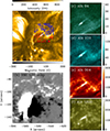 |
Fig. 1. Overview observations of the LTB. (a) Manifestation of the LTB at 02:37 UT in the AIA 171 image, overlaid with the distribution of the magnetic field in the region of interest. (b) LOS magnetic fields from HMI in the corresponding area. The white areas (blue contours) indicate the magnetic field with a positive polarity, while black areas (red contours) indicate the magnetic field with a negative polarity. (c)–(f) Enlarged AIA images at four different bands in the region marked by the black box in panel a. The red and blue curves in panel a denote contours of the magnetic field with strengths of ±100 G, ±200 G, and ±300 G. |
Figs. 1c–1f show manifestations of the LTB in AIA 94 Å, 131 Å, 304 Å, and 1600 Å bands. Compared to other regions, the brightening was quite evident in these bands, indicating the multithermal nature of the LTB. The LTB displayed a distinct shape in high-temperature bands (i.e., AIA 94 and 131 bands, which correspond to the corona) and in low-temperature bands (i.e., AIA 304 and 1600 bands, which correspond to the chromosphere). As shown in Figs. 1c and 1d, the LTB exhibited the tadpole-like shape, but a stick-like shape in Figs. 1e and 1f. The brightening at the head of LTB might be caused by hot plasma and/or plasma accumulation. The observed discrepancy in shape suggests a nonuniform distribution of the plasma.
3.2. Performance and light curves of the LTB
Figure 2 presents the time evolution of the LTB in the (E)UV images. The brightening first appeared as a dot-shaped structure in IRIS 1400 images, and then extended perpendicular to the PIL (Fig. 1a). After 02:35 UT, the corresponding area in the high-temperature bands began to brighten as the dotted shape as well (Figs. 2a–2c). The observed structure exhibited distinct characteristics at close times (Fig. 2a vs. Fig. 2b vs. Fig. 2c vs. Fig. 2d), but presented a similar evolutionary process in the time series, that is, dot-like first, then loop-like, and back to dot-like, as shown in Figs. 2a1–2a4 vs. Figs. 2b1–2b4. The different shapes at close times between observational bands indicate that the heating occurred in stages. The change in the shape in one observational band reflects local plasma that is first heated and then cooled. It is important to note that the structure observed in the AIA bands seems to be just the middle portion of the brightening observed in IRIS SJI. The linear structure in AIA corresponds to a segment of the curved structure in IRIS, while the remainder was not observed by AIA. The discrepancy may have been caused by the plasma outside the response temperature of AIA bands.
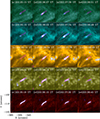 |
Fig. 2. Performances of the LTB in imaging observations. Manifestation of the LTB at different instants in each observed band, (a) AIA 94 Å band, (b) AIA 131 Å band, (c) AIA 171 Å band, (d) AIA 1600 Å band, and (e) IRIS/SJI 1400 Å band. The ellipse in panel b3 denotes the area based on which we calculated the emission light curves (Fig. 3) and the evolution of the maximum temperature and maximum emission measure (Fig. 7). The blue curves in panels a–e show the contours of the intensity at levels of 22 DN, 80 DN, 800 DN, 200 DN, and 280 DN. The pink curves in different AIA bands correspond to the contours of the SJI 1400 Å band. |
To illustrate the detailed heating and cooling process in each observational band, we calculated the emission within the area marked by the ellipse in Fig. 2. The corresponding results are shown in Fig. 3. The emission of the LTB significantly increased in two IRIS bands and in eight AIA bands, confirming the multithermal nature of the LTB. The light curves (LCs) exhibited a rapid increase followed by a gradual decrease, which is consistent with the observational features of UV bursts and Solar Orbiter campfires (e.g., Cai et al. 2019a; Nelson et al. 2023). The emission of the SJI 1330 band first increased and then peaked at 02:34:50 UT, which is earlier than the peak time of 02:35:36 UT in the AIA 1600 band and in the SJI 1400 band. Considering the characteristic temperature of each band, the discrepancy between these curves displayed in Figs. 3a–3c implies that the release of energy related to the event might initially occur in the chromosphere-transition region.
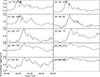 |
Fig. 3. Evolution of emission obtained in the area denoted by the ellipse in Fig. 2. The arrows denote the subpeaks. |
The time when the LC began to ascend is consistent in the seven AIA EUV bands, approximately at 02:35 UT. Subsequently, the AIA EUV bands peaked successively. The AIA 94 band reached its peak at 02:36:50 UT first, followed by the remaining bands, which reached their peaks after 02:37 UT. The temperature response functions of the AIA bands (Lemen et al. 2012) shows that the difference in peak in time suggests for the heating process that the plasma temperature evolved from lower than 105 K to at least 106 K. In addition, a subpeak was observed behind the primary peak in the LCs of the SJI bands and AIA 1600 band, as marked by the arrows in Figs. 3a–3c.
3.3. Space-time maps of the LTB
The LTB was extended in two directions in imaging observations (Fig. 2). In order to investigate the kinetic behavior of the LTB, we created space-time emission maps along the propagating path of the event using the AIA and IRIS images. Given the collimating ejection observed in AIA images (Fig. 2), the space-time brightness maps (Fig. 4) of the AIA bands were created along the major axis of the ellipse in Fig. 2b3. The LTB showed a clear brightening starting from 02:34 UT in the AIA 1600 band, and then presented an indeterminate extension in the opposite direction (Fig. 4a). Subsequently, plasma flows from the initial point repeatedly started at about 02:35 UT and 02:36 UT in other AIA EUV bands (Fig. 4). In coronal images, heated plasma predominantly moved in the southeast direction (Figs. 4b–4f). Unlike the results obtained from the coronal images, the LTB showed clear bidirectional flows in the map obtained from the AIA 304 images, as displayed by the arrows in Fig. 4g.
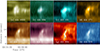 |
Fig. 4. Space-time brightness maps in different AIA and IRIS bands obtained along the major axis of the ellipse in Fig. 2. The arrows in panel g denote the bidirectional flows of LTB. |
Figure 5a shows the performance of the LTB at 02:36 UT in an IRIS/SJI 1400 image. Since the LTB geometry in IRIS observations is curved, the space-time map was created along the curved line named PQ in Fig. 5a. The change in length is easily discernible from the map. From the slope of the front of brightening, we found that the LTB spread northwest in the sky plane at a speed of about 6.4 km s−1. The southeast extension increased in speed at 02:44:30 UT, changing from 12.9 km s−1 to 45.1 km s−1. On the other hand, the contour curves in Fig. 5a indicate three bright kernels in the spine of the LTB, which might correspond to plasma blobs caused by the tearing mode instability. Figs. 5c–5k present the emission distribution at the position marked by the short bars, from which we can clearly identify the plasma blobs. These plasma blobs were formed during the period of 02:34 UT–02:35 UT, in which the LCs (Fig. 3) and flow speed (Fig. 5b) increased notably.
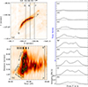 |
Fig. 5. Performances of the LTB in IRIS SJI images. (a) SJI 1400 image overlaid with contours to denote the brightness kernels. The raster numbers 5, 6, and 7 are plotted. (b) Space-time brightness map obtained along the dotted line PQ in panel a. The intensity is on an inverse scale. (c)–(k) Intensity distribution in the instance marked by the short solid line in panel b. The black lines in panel a denote the position of the IRIS slits. |
3.4. Temperature and emission measure
Fig. 6 shows the thermal manifestation of the LTB derived with the DEM method at 02:36:03 UT and 02:37:39 UT, including EM distributions integrated in the set temperature range (Figs. 6a1–6a4 and 6b1–6b4), total EM (Figs. 6a5 and 6b5), and the average EM temperature (Figs. 6c and 6d). At 02:36:03 UT, the EM is enhanced in the temperature intervals 2.2−4.5 MK (Fig. 6a2), 5−7.1 MK (Fig. 6a3), and 8−10 MK (Fig. 6a4), but at different positions. The crosses marked by the vertical and horizontal lines serve as references to confirm the enhancement position. The enhancement was located in the northwest corner in Fig. 6a2, but at the crosses in Figs. 6a3 and 6a4. This result is consistent with the EUV observations by AIA (Fig. 1), indicating that the LTB had a hot head and a cooler body. At 02:37:39 UT, the EM was enhanced in intervals of 1−2 MK, 2.2−4.5 MK dominated, and 5−7.1 MK. Unlike the manifestations in Fig. 6a2, hot and cooler plasma mixed together at the head of the LTB. The emission from body of the LTB was mainly contributed by plasma with a temperature lower than 4.5 MK.
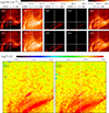 |
Fig. 6. Thermal characteristics of the LTB. (a1)–(a5): EM at different temperature intervals at 02:36:03 UT. (b1)–(b5): Same as panels (a1)–(a5) at 02:37:39 UT. (c) and (d): EM average temperatures obtained at 02:36:03 UT (c) and 02:37:39 UT (d). The crosses given by the vertical and horizontal lines indicate the head of the LTB in AIA images. |
According to Eq. (2), EM average temperature maps of the LTB were obtained (Figs. 6c and 6d). As expected, the temperature of the head was higher than that of the body at both times. The mean temperature around the head was approximately 3.2 × 10⁶ K at 02:36:03 UT, which is slightly higher than the temperature of about 2.96 × 10⁶ K at 02:37:39 UT.
Figure 7 shows the evolution of the maximum temperature and the maximum EM obtained from the ellipse versus time during the analyzed period. The maximum plasma temperature inside the jet can reach 5.4 × 10⁶ K. Both curves exhibit an almost simultaneous slow increase and rapid decrease, which is opposite to the change of the LCs in Fig. 3. The moment when temperature and EM begin to increase is consistent with the instant when the AIA high-temperature band curves (e.g., AIA 94 Å and 131 Å bands) increase, but it is about one minute later than the low-temperature bands (i.e., the IRIS SJI bands and the AIA 1600 band). The increasing temperature and EM means that the brightness increase is probably caused by plasma heating and plasma accumulation.
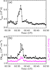 |
Fig. 7. Change in the maximum temperature and maximum EM in the area marked by the ellipse in Fig. 2 vs. time. The pink curve shows the change in the derived density. |
On the other hand, assuming that the depth (l) of the emitting plasma in LOS is equal to the widths of the LTB, we can derive ne using Eq. (1). Since ne depends on the selection of l, we used l = 1000 km here to investigate the relative change in density over time. Based on the derived distributions of EM (Fig. 6a5 and 6b5), we found that ne at the head of the LTB was larger at 02:37:39 UT than that at 02:36:03 UT, which had densities of about 1.7 × 1010 cm−3 and 1.45 × 1010 cm−3, respectively. This might indicate that plasma was accumulated at the head of the LTB. The lower temperature of the LTB at 02:37:39 UT compared to the temperature at 02:36:03 UT may be due to the enhanced radiation cooling caused by the higher density. The pink curve in Fig. 7b shows the variation in density derived from the EM. During the brightening process, ne increased by 1.38 times at most.
3.5. Spectrum of the LTB
Fig. 8 displays the performance of different spectral lines at 02:35:00 UT (panels a–e) and 02:35:56 UT (panels f–j). The white profile in each panel represents the distribution of the interested spectral line at the position marked by the short bars in Figs. 8a and 8f. Based on the formation temperature of spectral lines denoted in Sect. 2, we can analyze the heating of various components of the plasma in the LTB by comparing the performance of these spectral lines. The intensity of the chromosphere (C II, Mg II h&k) and transition region lines (O IV, Si IV) significantly increased compared with the background, suggesting that the plasma in the LTB could be heated to the temperature of the transition region. In Figs. 8b and 8g, the high-temperature coronal line Fe XXI 1354.08 Å did not show detectable emission in the brightening area, indicating that the plasma in the structure was not heated up to 107 K. Different from the temperature information given by the AIA images and the DEM method, the spectrum in Fig. 8 indicates the existence of plasma with temperature lower than 105 K in LTB.
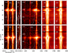 |
Fig. 8. Performances of the spectrum. The spectral data in the five main windows of the IRIS at 02:35:00 UT (a–e) and 02:35:56 UT (f–j). The former was obtained at the position of raster 7, and the latter was obtained at the position of raster 5. The lines on which we focus in each panel are C II 1334.53/1335.71 Å (a, f), Fe XXI 1354.08 Å (b, g), Si IV 1402.77 Å (c, h), and Mg II k&h 2796.35/2803.52 Å (d&e, i&j). The white curve in each panel shows the intensity profile obtained at the site denoted by the short white bar in panels a and f. |
In addition to the temperature, the morphology of LTB can also be understood based on the behaviors of the spectrum. The spectral lines were spatially tilted along the slit. The overall profiles of the spectral lines were blueshifted at the upper side of the LTB (Figs. 8a–8e), whereas they were redshifted at the lower side of the LTB (Figs. 8f–8j). In particular, the spatial tilt of the spectrum exhibits opposite direction in Figs. 8a–8e and Figs. 8f–8j. The spatial tilt was from northeast to southwest at 02:35:00 UT, but it was from northwest to southeast at 02:35:56 UT.
Figure 9 shows the details of the Si IV 1402 Å line at different times at three raster locations. We caution that the slit scanned from east to west (i.e., from raster 5 to raster 7), while the LBT plasma flowed east (i.e., from raster 7 to raster 5), as displayed in Figs. 2 and 4. Raster 5 scanned the spine of the LTB, and raster 7 scanned the area near the initial brightening site of the LTB. Compared to Figs. 9b and 9h, the intensity of the Si IV line at raster 6 (Figs. 9e and 9f) was mainly concentrated near the line center, with a slight spatial tilt as well. Considering the specific locations that extract the spectral data, the discrepancies shown in Fig. 8 could be caused by diverse mechanisms, which we discuss further in Sect. 4.
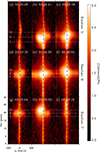 |
Fig. 9. Representation of the Si IV line at different times and different locations. The dotted white lines in each panel mark the position from which we extracted the spectral lines. The vertical black lines denote the line center of the Si IV line. |
To check the motion along the LOS and the turbulent state of the LTB, individual spectral profiles of the Si IV 1402 Å line at the positions denoted by horizontal dotted white lines in Fig. 9 were extracted, as the black curves display in Fig. 10. The spectral profile in Fig. 9(h)II was different from the profiles obtained at other positions, showing an obvious multipeak characteristic. Except for the profile showed in Fig. 10(h)II, the spectral profiles basically consisted of a sharp center and broad wings. Excess emission was observed in both wings of the Si IV profiles at these sites (e.g., Figs. 10(b)I, 10(d)II, and 10(h)II), which implies an additional flow component and/or turbulence in the interested area (e.g., Innes et al. 1997; Cai et al. 2019a; Li & Peter 2019).
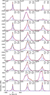 |
Fig. 10. Double-Gaussian fitting results of the Si IV line profiles, except for panel hII. The solid red, blue, purple, and yellow lines represent the overall profiles and the fitting components. The Doppler velocity (first row) and the derived nonthermal velocity (second row) of each component are presented in the panels. |
Figure 10 shows the corresponding fitting profiles and the derived Doppler velocity and nonthermal velocity with the individual components described in Eq. (3). Considering the multipeak characteristic, we employed a triple-Gaussian function, that is, we added a third Gaussian function to the right of Eq. (3), to fit the spectral profile in Fig. 10(h)II. We discuss the fitting results in Fig. 10 from two aspects. First, comparing Figs. 10(a)I–10(e)I with Figs. 10(a)III–10(e)III, the signs of the Doppler velocities were opposite, indicating that the plasma flows in the LOS were opposite at the lower and upper side of the LTB, which is the signal of twisting motion (De Pontieu et al. 2014b; Cheung et al. 2015b). In Figs. 10g–10i, the Doppler velocities of both components are negative. It suggests that the plasma in the LTB at the position of raster 7 primarily flowed upward. The spectral line at individual positions showed a multipeak profile with a high redshift and blueshift component (Fig. 10(h)II), which might be related to the magnetic reconnection.
Second, the LTB was a turbulent structure, regardless of the sampling location. At locations such as shown in Figs. 10(b)II, 10(h)II, and 10(h)III, the fitting curves affected the center of the observed spectral profiles well, implying that LTB had a high nonthermal velocity that can reach 90 km s−1. It should be noted here that the portion of the nonthermal velocities given in Fig. 10 cannot entirely demonstrate the turbulent state of the LTB. When fitting the spectral profiles with a double-Gaussian function, one component would have a strong line broadening in order to fit the additional radiation at the line wings (e.g., Figs. 10e, 10(g)I, and 10(h)I). The excess radiation at the line wings might be related to several options, such as the continuous distribution of plasma velocity and non-Maxwellian ion distribution (e.g., Dudík et al. 2017; Ni et al. 2021). Therefore, to some extent, these derived nonthermal broadenings were not naturally related to the turbulence in the LTB.
In addition, by examining the relation between the ratio of the intensity of the O IV doublet lines and the electron density (Fig. 8a in Cai et al. 2019a), we can estimate the electron density of the LTB. Based on the intensity of the O IV doublet lines extracted at the positions of raster 5, raster 6, and raster 7, we obtained the density evolution (Fig. 11). The density was in a range from 1.37 × 1010 cm−3 to 2.2 × 1011 cm−3, with the mean value of about 8.25 × 1010 cm−3. Since the value of 1.12 × 109 cm−3 falls outside the reasonable diagnostic density range (it is more accurate between 3.16 × 109 cm−3 and 3.16 × 1011 cm−3, given by Cai et al. 2019a), we did not use it in the calculation process. The values are close to observations of various small-scale brightening events, but they are higher than the values derived from the DEM method. The discrepancy between the two methods might be caused by a combination of various factors.
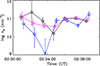 |
Fig. 11. Electron density (ne) of the LTB estimated at positions of raster 5 (black curve), raster 6 (pink curve), and raster 7 (blue curve). |
When only AIA images are used for DEM calculation, the constraint on the high-temperature component tends to be weaker (Su et al. 2018). Compared to the DEM results obtained by incorporating XRT data that are sensitive to hotter plasma, the temperatures and EM derived from the former method might be lower (Reeves et al. 2020). This might be one reason for the density estimated from the DEM method to be lower than that derived from the O IV line ratios. On the other hand, when using the DEM method and the ratio of O IV spectral lines to calculate the density, hypotheses are inevitably induced (e.g., Cheng et al. 2012; Cai et al. 2019a; Reeves et al. 2020). Usually, we need to assume the depth of the brightening along the LOS as equal to its width in the DEM method. Additionally, we did not add the factor of 0.83 (the hydrogen relative to the electron density) in Eq. (1), which leads to the drop-off of the density. We note that forms of Eq. (1), with and without the factor, have been commonly used in studies (e.g., Cheng et al. 2012; Reeves et al. 2020). For the O IV doublet line method, Cai et al. (2019a) discussed the variation in the density versus the formation temperature of the O IV lines. They concluded that when the electron density is deduced according to this method, the uncertainty in the density would be apparent when the object of interest includes multiple thermal components. Unfortunately, our previous analysis showed that the LTB had a multithermal structure. In addition, the theoretical relation between the electron density and the intensity ratio of the O IV lines was typically obtained under the assumption of ionization equilibrium and the element abundance of the photosphere or corona (Dudík et al. 2017; Cai et al. 2019a). It might also introduce an uncertainty in the derived density.
4. Discussion
We mainly studied the evolution of an LTB that took place on February 28, 2014, based on the imaging and spectral data provided by IRIS and SDO. The LTB presented a clear brightening in multiple (E)UV bands and exhibited a bidirectional flow perpendicular to the PIL. The structure observed in the AIA bands appears to be the middle portion of the LTB observed in IRIS/SJI. The unobserved part at two sides might arise because the energy was insufficient to heat the dense plasma to a high temperature (Chen et al. 2021). The chromosphere (C II, Mg II h&k) and transition region lines (O IV, Si IV) and the DEM analysis imply that the LTB consisted of plasma with a temperature of 104 K to 106.7 K, that is, a multithermal structure. The LCs showed a delay of about one minute between the low- and high-temperature bands, indicating continuous heating through magnetic reconnection that raised the plasma in the lower atmosphere to a higher temperature.
4.1. Category of the LTB
Small-scale brightening events are ubiquitous in the solar atmosphere. They are classified into different types based on features such as the spatial scale, lifetime, energy, spectral performances, and formation mechanism (e.g., Tian et al. 2016; Chen et al. 2021). Priest (2014) outlined the observational features of ARTBs, which possess areas of 10−100 Mm2, lifetimes of 1−15 minutes, plasma temperatures of 5 MK, a point-like or loop-like shape, energies of 1024–1029 erg, and primarily occur around sunspots. For the characteristics mentioned above, the LTB fell into this category in terms of the characteristics of size (∼9.46 Mm2), density (∼8.25 × 1010 cm−3), temperature (∼5.4 MK), loop-like shape, and the occurrence area around sunspots. The feature that distinguishes between ARTBs and the LTB we analyzed lies in the formation height. Aschwanden (2005) and Priest (2014) pointed out that ARTBs mainly occur at the coronal height. The LTB here was first observed in AIA 1600 Å band, which corresponds to the chromosphere, and in the IRIS 1400 Å band, which corresponds to the transition region. It then appeared in other coronal AIA bands. This indicates that the plasma at a lower height was heated first. Therefore, combining observations in images and the spectrum, we speculate that an LTB resulting from magnetic reconnection probably occurs in the upper chromosphere-transition region.
We classified the LTB as ARTB based on various observational characteristics. Similarities between the LTB and other transient heating events exist as well. The evolution of the light curves displays a similar trend to that of UV bursts (Smitha et al. 2018). The LTB was morphologically like the loop-like structures observed by Hi-C and Solar Orbiter, showing extension characteristics (Tiwari et al. 2019; Berghmans et al. 2021). The plasma blobs observed in the LTB are an additional feature. Their appearance was close to the time at which the apparent velocity changed and the light curves increased. With the spectral data provided by IRIS, we found that the LTB twisted along its axis. The similarities and differences among the different types of heating events are closely related to the occurrence height and area and to the magnetic field environment (Yan et al. 2015; Ni et al. 2016; Tian et al. 2016). For example, the observed loop-like structure is similar to the campfires in propagation speed, apparent shape, and brightness evolution. The LTB occurred in active regions and campfires occurred in quiet regions, however, resulting in the difference in released energy between the two, which accordingly corresponds to the difference in plasma temperature.
4.2. Possible magnetic configuration
Transient heating events are typically associated with magnetic reconnection, but with differences in the predistribution of the magnetic field and the rearrangement of field lines during the reconnection process. Through horizontal motions or rotations in the photosphere, a bundle of magnetic loops might become intertwined along the axial direction and form a braided magnetic structure. As degree of tangling increased, energy would be released as a result of magnetic reconnection (Cirtain et al. 2013; Pontin et al. 2017; Chen et al. 2021). The formation of campfires is thought to be related to this magnetic configuration (e.g., Chen et al. 2021). A similar scenario is that two neighboring magnetic loops with small relative angles or opposite direction might approach each other upon being disturbed, leading to magnetic reconnection at the approach point (e.g., Chae et al. 2000; Xue et al. 2016). Magnetic flux emergence and/or cancellation in active regions is correlated with the generation of numerous small-scale brightening events, such as explosive events and UV bursts (e.g., Peter et al. 2014; Cai et al. 2019a; Huang et al. 2019). Magnetic reconnection takes place between the emerging magnetic flux or the moving magnetic structures and the preexisting background magnetic fields (e.g., Yokoyama & Shibata 1996; Ni et al. 2017; Cai et al. 2019a). Yokoyama & Shibata (1996) pointed out that the formation of a two-sided-loop structure is facilitated when the background field is approximately horizontal. The conversion of magnetic energy into thermal energy and kinetic energy leads to the heating of plasma in the lower atmosphere to coronal temperatures. This is observed as enhanced EUV emission and opposite-direction horizontal plasma flows.
The LTB appeared as a single magnetic structure in both IRIS and AIA imaging observations, and it is therefore unlikely that it was caused by a braided magnetic field. If the LTB were caused by the reconnection between two neighboring loops, two separate loop structures should be observed in images prior to the reconnection (e.g., Xue et al. 2016). However, no such structures were observed in the AIA and IRIS images. Based on the evolution of photospheric magnetic field in the corresponding area and based on the conclusion that the LTB belongs to ARTBs, we consider that the LTB was more likely generated by the emergence and/or cancellation of magnetic flux in the photosphere. The magnetic field in the moss region of sunspots is complex, and we cannot accurately determine the magnetic topology. The two possibilities can therefore not be entirely ruled out.
4.3. Role of plasma blobs
Several bright kernels were observed in the spine of the LTB (Fig. 5). They might be the counterpart of the plasma blobs that were caused by the tearing-mode instability. The variation in emission during the LTB, characterized by a rapid increase and slow decrease (Fig. 3), is closely aligned with the appearance of the plasma blobs (Fig. 5). Furthermore, the change in the apparent flow speed (Fig. 5b) also coincides with the appearance of these plasma blobs. Theories and numerical experiments have demonstrated a tight relation between MR and plasma blobs, that is, MR increases sharply as plasmoids form, followed by a slow decrease in an oscillating pattern (Shen et al. 2011; Ni et al. 2015b). Direct observational evidence that magnetic islands facilitate the release of magnetic energy is scarce. Our results might provide direct evidence that supports the role of plasma blobs in accelerating the release of magnetic energy. The direct effect of the large MR includes enhanced flaring emission and an increased speed of the plasma flows, which are more significant in CME-flare eruptions (e.g., Ko et al. 2003; Cai et al. 2019b). These results not only underscore the importance of plasma blobs in the release of magnetic energy, but also suggest that the large-scale eruptions and small-scale transient brightenings are similar.
In the reconnection process, the magnetic energy was converted into thermal and kinetic plasma energy. The physical parameters of the heating event obtained in Sect. 3 allowed us to estimate the energy required to heat and accelerate the plasma in the LTB. The thermal energy (Et) and the kinetic energy (Ek) can be formulated as Et = 3/2nekBTV and Ek = 1/2ρv2V, where kB, T, ρ, v, and V are the Boltzmann constant, the temperature, the plasma mass density, the velocity, and the volume of the source region, respectively. The velocity can be derived from the apparent flow (∼45.1 km s−1 in Fig. 5) and the Doppler velocity (∼108.6 km s−1 in Fig. 10), so that v = 117.6 km s−1. Assuming the brightening was a cylinder and its width equalled its depth, the volume V = 1.6 × 10¹⁹ m3 based on Fig. 2. The results for the other parameters obtained earlier were T = 5.4 × 10⁶ K, ne = 8.25 × 1010 cm−3. Substituting these values into Et and Ek gives Et = 1.47 × 10²⁰ J and Ek = 1.53 × 10¹⁹ J, which are also within the energy range of ARTBs. The temperature and velocities we used to calculate the thermal and kinetic energy are the upper limits, which means that both energies might be overestimated. In addition, the LTB occurred in the moss region of a sunspot. The mean value of the LOS magnetogram in the area denoted by the box in Fig. 1b was about 100 G, providing an essential magnetic environment for the conversion of magnetic energy into thermal energy and kinetic energy.
The LCs shown in Figs. 3a–3c present a double-peak feature, similar to the evolution of MR of two-sided loop-type jets revealed by Yokoyama & Shibata (1996). In their study, where magnetic reconnection occured between the overlying horizontal magnetic field and emerging magnetic field, the first peak in the MR curve is related to the anomalous resistivity caused by the formation of plasmoids, and the second peak is associated with the enhanced inflows driven by a pressure gradient resulting from the plasmoid movement. The generation of the first peak can be confirmed by the coincidence of the appearance time of plasma blobs and the variation in velocity and light curves. The second peak was uncertain in observations because it might have been produced by a new impulsive burst in the lower atmosphere. MR reflects the energy-transforming speed from magnetic to thermal and kinetic energy. The measurement of MR versus time is crucial in the context of solar eruptions. Current methods for its measurement include using the ratio of the inflow and outflow speed of magnetic reconnection (e.g., Lin et al. 2005; Cai et al. 2021), the ratio of the thickness and length of CS (e.g., Xue et al. 2018), or the time derivative of the reconnected magnetic flux (e.g., Takahashi et al. 2017). Limited by the instruments and observational conditions, as well as by the simple topology and the short lifetime of the small-scale brightening events, it is difficult to give the evolution of MR. The derived thermal energy of the LTB was nearly an order of magnitude higher than its kinetic energy, implying that most of the released magnetic energy was converted into thermal plasma energy in small-scale heating events (Yokoyama & Shibata 1996). Considering the formation mechanism and the tangible manifestations of the LTB, to some extent, the LCs might be useful for reflecting the trend of MR in TBs.
4.4. Spectral performances
Two scenarios were analyzed in Sect. 3.5. The first scenario is that the spectral profiles were extracted at fixed sampling positions, corresponding to the results presented in Fig. 10. The spectral profiles exhibited asymmetric characteristics in the line wings (e.g., Figs. 10bII and 10hII), which arise from various factors, such as the multidirectional flows, and the uneven distribution of the temperature and density caused by the instability. Small-scale brightening events frequently display an asymmetry in their spectral line profiles (e.g., Innes et al. 1997, 2015; Cai et al. 2019a). To explain the possible origin of the asymmetry in spectral profiles, researchers performed MHD simulations of magnetic reconnection and then synthesized the Si IV spectrum (Innes et al. 2015; Cai et al. 2019a; Ni et al. 2021). They concluded that the complex motions of magnetic plasmoids generated by magnetic reconnection might affect the spectral line profiles and cause them become asymmetrical. Although these numerical experiments used different initial settings, the role of the plasmoids in the formation of the asymmetry profiles was consistent. Except for magnetic islands, the vortex-like structures produced by the Kelvin-Helmholtz instability could disturb the distribution of magnetic fields and plasmas, resulting in high-temperature and high-density cores (Ni et al. 2017). This complex plasma environment might also create the observed bright kernels in AIA and IRIS, and it might affect the profile of spectral lines.
The second scenario is that spectral profiles were compared that were extracted at different sampling positions. The overall profiles of the spectral lines at the upper and lower edges of the structure were dominated by redshift and blueshift, respectively, such as Figs. 10b, 10d, and 10e, indicating that the structure might be rotating (e.g., De Pontieu et al. 2014b; Cheung et al. 2015b; Li & Peter 2019). Combined with the apparent flow observed in imaging data, we suggest that the plasma in the LTB might exhibit a helical flow pattern, which could be ubiquitous in small-scale events, as proposed by De Pontieu et al. (2014b). Li & Peter (2019) analyzed the details of an Si IV 1394 Å line that was emitted from a cool coronal loop, and found a spatial tilt from one footpoint of the loop to the other. They considered that the spatial tilt of the spectrum was an indication of the helical structure, which was produced by the ejection of helicity at the loop footpoint. These results indicate that the small-scale events observed in imaging observations contain additional motions such as helical flows and bidirectional flows, as well as turbulent structures.
The Doppler-shift signals in Fig. 10 indicate that the plasma in LTB changed from an upward motion (blueshift) to a rotational motion (redshift and blueshift at opposite boundaries of the LTB) as the sampling moved from the initial brightening site to the spine (Fig. 10). Considering the space-time maps shown in Sect. 3.3, where raster 7 may have scanned the area near the magnetic reconnection, we propose two different mechanisms to explain these spectral features. (1) Rotating process of the LTB: The slanted distribution in the blue- and redshift components might be caused by the twisting motion of the LTB (Li & Peter 2019). This corresponds to the scenario in which the slit observed the spine of the LTB, indicating that the plasma not only flowed along the spine in the plane of the sky, but was also twisted. (2) Magnetic reconnection: When the slit scanned the region undergoing magnetic reconnection, the outflows from the reconnection both far away from and toward the Sun might cause the asymmetric feature in the spectral profiles (Innes et al. 1997). The reconnection process is known to produce high-speed outflows and can influence the Doppler shift of the spectral lines. These proposed mechanisms highlight the complexity of the observed spectral features and suggest that multiple processes contributed to the dynamics of the LTB.
The spectral profile of the C II and Mg II h&k lines also changed significantly, reflecting variations in the chromospheric plasma environment (Leenaarts et al. 2013; Rathore et al. 2015). The peak separation in the Mg II h&k line increased (Fig. 8), revealing the increase in the velocity gradient in the middle chromosphere. The blue peaks of Mg II h&k were stronger than the red peaks in Figs. 8i and 8j, while the opposite was observed in Figs. 8d and 8e. This distinction might be related to material flows in different directions in the chromosphere, which can be confirmed from the position of the emitting area.
5. Conclusions
Using the imaging data and spectrum of an active region observed by SDO and IRIS, we studied the thermal and dynamical evolution of a loop-like transient brightening by investigating the space-time maps and light curves of multiple observational bands covering the temperature range from 104 K to 107 K, as well as the details of the spectral profiles of the Si IV 1402 Å line. The LTB extended from a point-like to a linear structure, and exhibited bidirectional flow characteristics. The profiles of the Si IV line were clearly enhanced and asymmetrical. Our main findings are listed below.
-
(1)
Several bright plasma blobs were recognized in the spine of the LTB. Their appearance time was close to the increase in the apparent flow speed and light curves. This directly provides observational evidence for the important role of plasma blobs in the release process of magnetic energy.
-
(2)
The Si IV spectrum exhibited clear spectral tilt characteristics, and the Doppler velocities at the upper and lower sides of the LTB changed in sign, which might indicate a helical flow of the LTB based on a combination of the apparent flows in the images. The profiles of the Si IV line are strongly nonthermally broadened, indicating the turbulent state of the plasma inside the LTB.
Plasma blobs and helical motion are often observed in phenomena such as jets, surges, and CME-flare current sheets (e.g, Cai et al. 2015; Cheung et al. 2015b; Shen 2021). The results obtained in our work provide fundamental information for understanding the energy-release process in large-scale eruptions.
Going forward, Hi-C and Solar Orbiter/EUI have provided high-resolution imaging data that revealed fine magnetic structures in the corona. This raises the question whether even more intricate structures exist. Therefore, it is highly desirable to plan and construct the next generation of imaging telescopes with an even higher spatial resolution, such as the Solar Close Observations and Proximity Experiments (SCOPE, Lin et al. 2019). They may help us gain a more nuanced understanding of the questions of magnetic reconnection and solar atmospheric heating. Future studies are essential for a more detailed understanding of the release and conversion of energy in small-scale heating events, which will shed light on their role in the heating of the solar atmospheres. Advances in observational capabilities, coupled with sophisticated modeling and simulations, will contribute to unravelling the complexities of these intriguing solar phenomena.
Acknowledgments
We acknowledge the constructive comments and patience of an anonymous referee that helped to improve the manuscript. This work was supported by grants from the National Scientific Foundation of China (NSFC 12203020, 12473059), the Yunnan Key Laboratory of Solar Physics and Space Science (202205AG070009), Project of Central Plains Science and Technology Innovation Leading Talents of Henan Province (244200510012), and the Key research and development program of Henan province (231111222200). W.J. was supported by the Yunnan Science Foundation of China (202301AT070347) and the Strategic Priority Research Program of the Chinese Academy of Sciences (XDB0560000). We appreciate the teams of IRIS and SDO for their open data use policy. CHIANTI is a collaborative project involving George Mason University, the University of Michigan (USA) and the University of Cambridge (UK).
References
- Aschwanden, M. J. 2005, Physics of the Solar Corona. An Introduction with Problems and Solutions, 2nd edn. (Chichester: Praxis Publishing Ltd.) [Google Scholar]
- Berghmans, D., Auchère, F., Long, D. M., et al. 2021, A&A, 656, L4 [NASA ADS] [CrossRef] [EDP Sciences] [Google Scholar]
- Brekke, P., Hassler, D. M., & Wilhelm, K. 1997, Sol. Phys., 175, 349 [Google Scholar]
- Cai, Q. W., Wu, N., & Lin, J. 2015, Acta Astron. Sinica, 56, 598 [Google Scholar]
- Cai, Q., Shen, C., Ni, L., et al. 2019a, J. Geophys. Res.: Space Phys., 124, 9824 [NASA ADS] [CrossRef] [Google Scholar]
- Cai, Q., Shen, C., Raymond, J. C., et al. 2019b, MNRAS, 489, 3183 [Google Scholar]
- Cai, Q., Feng, H., Ye, J., & Shen, C. 2021, ApJ, 912, 79 [CrossRef] [Google Scholar]
- Chae, J., Wang, H., Goode, P. R., Fludra, A., & Schühle, U. 2000, ApJ, 528, L119 [NASA ADS] [CrossRef] [Google Scholar]
- Chen, P. F., & Priest, E. R. 2006, Sol. Phys., 238, 313 [Google Scholar]
- Chen, Y., Tian, H., Peter, H., et al. 2019, ApJ, 875, L30 [NASA ADS] [CrossRef] [Google Scholar]
- Chen, Y., Przybylski, D., Peter, H., et al. 2021, A&A, 656, L7 [NASA ADS] [CrossRef] [EDP Sciences] [Google Scholar]
- Cheng, X., Zhang, J., Saar, S. H., & Ding, M. D. 2012, ApJ, 761, 62 [NASA ADS] [CrossRef] [Google Scholar]
- Cheng, X., Li, Y., Wan, L. F., et al. 2018, ApJ, 866, 64 [Google Scholar]
- Cheung, M. C. M., Boerner, P., Schrijver, C. J., et al. 2015a, ApJ, 807, 143 [Google Scholar]
- Cheung, M. C. M., De Pontieu, B., Tarbell, T. D., et al. 2015b, ApJ, 801, 83 [Google Scholar]
- Cirtain, J. W., Golub, L., Winebarger, A. R., et al. 2013, Nature, 493, 501 [NASA ADS] [CrossRef] [Google Scholar]
- Curdt, W., & Tian, H. 2011, A&A, 532, L9 [NASA ADS] [CrossRef] [EDP Sciences] [Google Scholar]
- Del Zanna, G., Dere, K. P., Young, P. R., Landi, E., & Mason, H. E. 2015, A&A, 582, A56 [NASA ADS] [CrossRef] [EDP Sciences] [Google Scholar]
- De Pontieu, B., Title, A. M., Lemen, J. R., et al. 2014a, Sol. Phys., 289, 2733 [Google Scholar]
- De Pontieu, B., Rouppe van der Voort, L., McIntosh, S. W., et al. 2014b, Science, 346, 1255732 [Google Scholar]
- Dere, K. P., Landi, E., Mason, H. E., Monsignori Fossi, B. C., & Young, P. R. 1997, A&AS, 125, 149 [NASA ADS] [CrossRef] [EDP Sciences] [Google Scholar]
- Dudík, J., Dzifčáková, E., Meyer-Vernet, N., et al. 2017, Sol. Phys., 292, 100 [CrossRef] [Google Scholar]
- Freeland, S. L., & Handy, B. N. 1998, Sol. Phys., 182, 497 [Google Scholar]
- Gupta, G. R., & Tripathi, D. 2015, ApJ, 809, 82 [Google Scholar]
- Hong, J., Jiang, Y., Yang, J., et al. 2014, ApJ, 796, 73 [NASA ADS] [CrossRef] [Google Scholar]
- Hou, Z., Tian, H., Madjarska, M. S., et al. 2024, A&A, 687, A190 [NASA ADS] [CrossRef] [EDP Sciences] [Google Scholar]
- Huang, Z., Li, B., & Xia, L. 2019, Solar-Terr. Phys., 5, 58 [NASA ADS] [Google Scholar]
- Innes, D. E., Inhester, B., Axford, W. I., & Wilhelm, K. 1997, Nature, 386, 811 [Google Scholar]
- Innes, D. E., Guo, L. J., Huang, Y. M., & Bhattacharjee, A. 2015, ApJ, 813, 86 [Google Scholar]
- Joshi, R., Chandra, R., Schmieder, B., et al. 2020, A&A, 639, A22 [NASA ADS] [CrossRef] [EDP Sciences] [Google Scholar]
- Kahil, F., Hirzberger, J., Solanki, S. K., et al. 2022, A&A, 660, A143 [NASA ADS] [CrossRef] [EDP Sciences] [Google Scholar]
- Katsukawa, Y., Berger, T. E., Ichimoto, K., et al. 2007, Science, 318, 1594 [NASA ADS] [CrossRef] [Google Scholar]
- Kleint, L., Antolin, P., Tian, H., et al. 2014, ApJ, 789, L42 [NASA ADS] [CrossRef] [Google Scholar]
- Ko, Y.-K., Raymond, J. C., Lin, J., et al. 2003, ApJ, 594, 1068 [NASA ADS] [CrossRef] [Google Scholar]
- Lee, K. S., Moon, Y. J., Kim, S., et al. 2011, ApJ, 736, 15 [NASA ADS] [CrossRef] [Google Scholar]
- Lee, J.-O., Cho, K.-S., Lee, K.-S., et al. 2020, ApJ, 892, 129 [NASA ADS] [CrossRef] [Google Scholar]
- Leenaarts, J., Pereira, T. M. D., Carlsson, M., Uitenbroek, H., & De Pontieu, B. 2013, ApJ, 772, 90 [NASA ADS] [CrossRef] [Google Scholar]
- Lemen, J. R., Title, A. M., Akin, D. J., et al. 2012, Sol. Phys., 275, 17 [Google Scholar]
- Li, L. P., & Peter, H. 2019, A&A, 626, A98 [NASA ADS] [CrossRef] [EDP Sciences] [Google Scholar]
- Li, D., Ning, Z., & Su, Y. 2016, Ap&SS, 361, 301 [NASA ADS] [CrossRef] [Google Scholar]
- Lin, J., Ko, Y. K., Sui, L., et al. 2005, ApJ, 622, 1251 [NASA ADS] [CrossRef] [Google Scholar]
- Lin, J., Li, J., Forbes, T. G., et al. 2007, ApJ, 658, L123 [NASA ADS] [CrossRef] [Google Scholar]
- Lin, J., Wang, M., Tian, H., et al. 2019, Sci. Sin. Phys. Mech. Astron., 49, 059607 [Google Scholar]
- Mandal, S., Peter, H., Chitta, L. P., et al. 2021, A&A, 656, L16 [NASA ADS] [CrossRef] [EDP Sciences] [Google Scholar]
- Mandal, S., Chitta, L. P., Peter, H., et al. 2022, A&A, 664, A28 [NASA ADS] [CrossRef] [EDP Sciences] [Google Scholar]
- Martínez-Sykora, J., Rouppe van der Voort, L., Carlsson, M., et al. 2015, ApJ, 803, 44 [CrossRef] [Google Scholar]
- Nelson, C. J., Auchère, F., Aznar Cuadrado, R., et al. 2023, A&A, 676, A64 [NASA ADS] [CrossRef] [EDP Sciences] [Google Scholar]
- Ni, L., Lin, J., Mei, Z., & Li, Y. 2015a, ApJ, 812, 92 [Google Scholar]
- Ni, L., Kliem, B., Lin, J., & Wu, N. 2015b, ApJ, 799, 79 [Google Scholar]
- Ni, L., Lin, J., Roussev, I. I., & Schmieder, B. 2016, ApJ, 832, 195 [Google Scholar]
- Ni, L., Zhang, Q.-M., Murphy, N. A., & Lin, J. 2017, ApJ, 841, 27 [Google Scholar]
- Ni, L., Chen, Y., Peter, H., Tian, H., & Lin, J. 2021, A&A, 646, A88 [NASA ADS] [CrossRef] [EDP Sciences] [Google Scholar]
- Pesnell, W. D., Thompson, B. J., & Chamberlin, P. C. 2012, Sol. Phys., 275, 3 [Google Scholar]
- Peter, H. 2010, A&A, 521, A51 [NASA ADS] [CrossRef] [EDP Sciences] [Google Scholar]
- Peter, H., Tian, H., Curdt, W., et al. 2014, Science, 346, 1255726 [Google Scholar]
- Peter, H., Chitta, L. P., Chen, F., et al. 2022, ApJ, 933, 153 [NASA ADS] [CrossRef] [Google Scholar]
- Polito, V., Del Zanna, G., Dudík, J., et al. 2016, A&A, 594, A64 [NASA ADS] [CrossRef] [EDP Sciences] [Google Scholar]
- Pontin, D. I., Janvier, M., Tiwari, S. K., et al. 2017, ApJ, 837, 108 [NASA ADS] [CrossRef] [Google Scholar]
- Priest, E. 2014, Magnetohydrodynamics of the Sun (Cambridge: Cambridge University Press) [Google Scholar]
- Rathore, B., Carlsson, M., Leenaarts, J., & De Pontieu, B. 2015, ApJ, 811, 81 [NASA ADS] [CrossRef] [Google Scholar]
- Reeves, K. K., Polito, V., Chen, B., et al. 2020, ApJ, 905, 165 [NASA ADS] [CrossRef] [Google Scholar]
- Schou, J., Scherrer, P. H., Bush, R. I., et al. 2012, Sol. Phys., 275, 229 [Google Scholar]
- Shen, Y. 2021, Proc. Roy. Soc. London Ser. A, 477, 217 [NASA ADS] [Google Scholar]
- Shen, C., Lin, J., & Murphy, N. A. 2011, ApJ, 737, 14 [Google Scholar]
- Shibata, K., Nakamura, T., Matsumoto, T., et al. 2007, Science, 318, 1591 [Google Scholar]
- Smitha, H. N., Chitta, L. P., Wiegelmann, T., & Solanki, S. K. 2018, A&A, 617, A128 [NASA ADS] [CrossRef] [EDP Sciences] [Google Scholar]
- Su, Y., Veronig, A. M., Hannah, I. G., et al. 2018, ApJ, 856, L17 [NASA ADS] [CrossRef] [Google Scholar]
- Takahashi, T., Qiu, J., & Shibata, K. 2017, ApJ, 848, 102 [NASA ADS] [CrossRef] [Google Scholar]
- Takasao, S., Asai, A., Isobe, H., & Shibata, K. 2016, ApJ, 828, 103 [NASA ADS] [CrossRef] [Google Scholar]
- Tian, H., Xu, Z., He, J., & Madsen, C. 2016, ApJ, 824, 96 [CrossRef] [Google Scholar]
- Tiwari, S. K., Panesar, N. K., Moore, R. L., et al. 2019, ApJ, 887, 56 [NASA ADS] [CrossRef] [Google Scholar]
- Xue, Z., Yan, X., Cheng, X., et al. 2016, Nat. Commun., 7, 11837 [Google Scholar]
- Xue, Z., Yan, X., Yang, L., et al. 2018, ApJ, 858, L4 [Google Scholar]
- Yan, L., Peter, H., He, J., et al. 2015, ApJ, 811, 48 [NASA ADS] [CrossRef] [Google Scholar]
- Yan, X., Xue, Z., Jiang, C., et al. 2022, Nat. Commun., 13, 640 [NASA ADS] [CrossRef] [Google Scholar]
- Yokoyama, T., & Shibata, K. 1996, PASJ, 48, 353 [Google Scholar]
- Young, P. R., Tian, H., Peter, H., et al. 2018, Space Sci. Rev., 214, 120 [Google Scholar]
- Zhang, Q. M., & Ni, L. 2019, ApJ, 870, 113 [Google Scholar]
Appendix A: Spatial alignment of IRIS and AIA data
Since Si IV and C IV have similar formation temperatures and they are major contributors to the IRIS 1400 Å band and AIA 1600 Å band, respectively, the two bands have been used frequently for the spatial alignment of IRIS and AIA data. Our work also followed this approach.
Given the discoveries in Peter et al. (2022) that the parallel plasma loops observed in the Hi-C 172 Å high-temperature band and IRIS 1400 Å low-temperature band were spatial offset, here we used additional small-scale bright structures of less than 1″ that exist in hot and cool AIA images and IRIS images as calibration points to align the observational imaging data from the two instruments.
We spatially scaled the SDO observations to match the IRIS SJI 1400 Å band and aligned them using several brightening features, as presented in Fig. A.1(a)-A.1(c). The corresponding pixel size is 0.1667″ in Fig. A.1. Then, We utilized points A and B to align the AIA 1600 Å image and IRIS 1400 Å image, and points A and C to align AIA 1600 Å image and AIA 171 Å image. From Figs. A.1(d)-A.1(i), it is evident that these three sampling points exhibit minimal spatial offsets in both horizontal and vertical directions. Our primary concern here is whether the LTB studied here is composed of two parallel magnetic loops with high and cool temperatures, as researched by Peter et al. (2022). Therefore, we proceed by presenting the radiation distributions of the LTB at two distinct vertical positions (marked as D in Fig. A.1), as shown in Figs. A.1(j) and A.1(k). The emission peaks of the LTB in three observational bands were spatially consistent, indicating that the LTB in our work was likely to resemble the plasma loops discussed in Li & Peter (2019), rather than the parallel loops proposed in Peter et al. (2022).
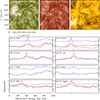 |
Fig. A.1. Spatial alignment between AIA 1600 Å, IRIS 1400 Å, and AIA 171 Å images. (a)-(c) The AIA and IRIS images at nearest times. The intensity in panels (a)-(c) are on an inverse scale. The horizontal and vertical lines at sampling points A, B, C, and D were used to determine the offset between observational bands. (d)-(k) The emission along the lines in panels (a)-(c). The black lines, red lines, and purple lines correspond to the emission of the AIA 1600 Å, the IRIS 1400 Å, and AIA 171 Å, respectively. The vertical pink lines denote the position of the sampling points. Abbreviation ’A-hor’ represents the horizontal line at point A, and the same applies to the others. Since we were only concerned with the changes in emission here, the vertical axis was not labelled with specific scales. |
All Figures
|
Fig. 1. Overview observations of the LTB. (a) Manifestation of the LTB at 02:37 UT in the AIA 171 image, overlaid with the distribution of the magnetic field in the region of interest. (b) LOS magnetic fields from HMI in the corresponding area. The white areas (blue contours) indicate the magnetic field with a positive polarity, while black areas (red contours) indicate the magnetic field with a negative polarity. (c)–(f) Enlarged AIA images at four different bands in the region marked by the black box in panel a. The red and blue curves in panel a denote contours of the magnetic field with strengths of ±100 G, ±200 G, and ±300 G. |
| In the text | |
|
Fig. 2. Performances of the LTB in imaging observations. Manifestation of the LTB at different instants in each observed band, (a) AIA 94 Å band, (b) AIA 131 Å band, (c) AIA 171 Å band, (d) AIA 1600 Å band, and (e) IRIS/SJI 1400 Å band. The ellipse in panel b3 denotes the area based on which we calculated the emission light curves (Fig. 3) and the evolution of the maximum temperature and maximum emission measure (Fig. 7). The blue curves in panels a–e show the contours of the intensity at levels of 22 DN, 80 DN, 800 DN, 200 DN, and 280 DN. The pink curves in different AIA bands correspond to the contours of the SJI 1400 Å band. |
| In the text | |
|
Fig. 3. Evolution of emission obtained in the area denoted by the ellipse in Fig. 2. The arrows denote the subpeaks. |
| In the text | |
|
Fig. 4. Space-time brightness maps in different AIA and IRIS bands obtained along the major axis of the ellipse in Fig. 2. The arrows in panel g denote the bidirectional flows of LTB. |
| In the text | |
|
Fig. 5. Performances of the LTB in IRIS SJI images. (a) SJI 1400 image overlaid with contours to denote the brightness kernels. The raster numbers 5, 6, and 7 are plotted. (b) Space-time brightness map obtained along the dotted line PQ in panel a. The intensity is on an inverse scale. (c)–(k) Intensity distribution in the instance marked by the short solid line in panel b. The black lines in panel a denote the position of the IRIS slits. |
| In the text | |
|
Fig. 6. Thermal characteristics of the LTB. (a1)–(a5): EM at different temperature intervals at 02:36:03 UT. (b1)–(b5): Same as panels (a1)–(a5) at 02:37:39 UT. (c) and (d): EM average temperatures obtained at 02:36:03 UT (c) and 02:37:39 UT (d). The crosses given by the vertical and horizontal lines indicate the head of the LTB in AIA images. |
| In the text | |
|
Fig. 7. Change in the maximum temperature and maximum EM in the area marked by the ellipse in Fig. 2 vs. time. The pink curve shows the change in the derived density. |
| In the text | |
|
Fig. 8. Performances of the spectrum. The spectral data in the five main windows of the IRIS at 02:35:00 UT (a–e) and 02:35:56 UT (f–j). The former was obtained at the position of raster 7, and the latter was obtained at the position of raster 5. The lines on which we focus in each panel are C II 1334.53/1335.71 Å (a, f), Fe XXI 1354.08 Å (b, g), Si IV 1402.77 Å (c, h), and Mg II k&h 2796.35/2803.52 Å (d&e, i&j). The white curve in each panel shows the intensity profile obtained at the site denoted by the short white bar in panels a and f. |
| In the text | |
|
Fig. 9. Representation of the Si IV line at different times and different locations. The dotted white lines in each panel mark the position from which we extracted the spectral lines. The vertical black lines denote the line center of the Si IV line. |
| In the text | |
|
Fig. 10. Double-Gaussian fitting results of the Si IV line profiles, except for panel hII. The solid red, blue, purple, and yellow lines represent the overall profiles and the fitting components. The Doppler velocity (first row) and the derived nonthermal velocity (second row) of each component are presented in the panels. |
| In the text | |
|
Fig. 11. Electron density (ne) of the LTB estimated at positions of raster 5 (black curve), raster 6 (pink curve), and raster 7 (blue curve). |
| In the text | |
|
Fig. A.1. Spatial alignment between AIA 1600 Å, IRIS 1400 Å, and AIA 171 Å images. (a)-(c) The AIA and IRIS images at nearest times. The intensity in panels (a)-(c) are on an inverse scale. The horizontal and vertical lines at sampling points A, B, C, and D were used to determine the offset between observational bands. (d)-(k) The emission along the lines in panels (a)-(c). The black lines, red lines, and purple lines correspond to the emission of the AIA 1600 Å, the IRIS 1400 Å, and AIA 171 Å, respectively. The vertical pink lines denote the position of the sampling points. Abbreviation ’A-hor’ represents the horizontal line at point A, and the same applies to the others. Since we were only concerned with the changes in emission here, the vertical axis was not labelled with specific scales. |
| In the text | |
Current usage metrics show cumulative count of Article Views (full-text article views including HTML views, PDF and ePub downloads, according to the available data) and Abstracts Views on Vision4Press platform.
Data correspond to usage on the plateform after 2015. The current usage metrics is available 48-96 hours after online publication and is updated daily on week days.
Initial download of the metrics may take a while.