| Issue |
A&A
Volume 690, October 2024
|
|
|---|---|---|
| Article Number | A108 | |
| Number of page(s) | 19 | |
| Section | Extragalactic astronomy | |
| DOI | https://doi.org/10.1051/0004-6361/202348727 | |
| Published online | 03 October 2024 | |
Feedback-free starbursts at cosmic dawn
Observable predictions for JWST
1
Center for Astrophysics and Planetary Science, Racah Institute of Physics, The Hebrew University, Jerusalem 91904, Israel
2
Santa Cruz Institute for Particle Physics, University of California, Santa Cruz, CA 95064, USA
3
School of Physics and Astronomy, Tel Aviv University, Tel Aviv 6997801, Israel
4
Department of Space, Planetary & Astronomical Sciences and Engineering, Indian Institute of Technology, Kanpur 208016, India
5
University of Massachusetts Amherst, Amherst, MA 01003-9305, USA
6
Kavli Institute for Cosmology, University of Cambridge, Cambridge CB3 0HA, UK
7
Cavendish Laboratory, University of Cambridge, Cambridge CB3 0HE, UK
Received:
24
November 2023
Accepted:
20
March 2024
Abstract
Aims. We extend the analysis of a physical model within the standard cosmology that robustly predicts a high star-formation efficiency (SFE) in massive galaxies at cosmic dawn due to feedback-free starbursts (FFBs). This model implies an excess of bright galaxies at z ≳ 10 compared to the standard models based on the low SFE at later epochs, an excess that is indicated by JWST observations.
Methods. Here we provide observable predictions of galaxy properties based on the analytic FFB scenario. These can be compared with simulations and JWST observations. We use the model to approximate the SFE as a function of redshift and mass, assuming a maximum SFE of ϵmax = 0.2 − 1 in the FFB regime. From this, we derive the evolution of the galaxy mass and luminosity functions as well as the cosmological evolution of stellar and star-formation densities. We then predict the star-formation history (SFH), galaxy sizes, outflows, gas fractions, metallicities, and dust attenuation, all as functions of mass and redshift in the FFB regime.
Results. The major distinguishing feature of the model is the occurrence of FFBs above a mass threshold that declines with redshift. The luminosities and star formation rates in bright galaxies are predicted to be in excess of extrapolations of standard empirical models and standard cosmological simulations, an excess that grows from z ∼ 9 to higher redshifts. The FFB phase of ∼100 Myr is predicted to show a characteristic SFH that fluctuates on a timescale of ∼10 Myr. The stellar systems are compact (Re ∼ 0.3 kpc at z ∼ 10 and declining with z). The galactic gas consists of a steady wind driven by supernovae from earlier generations, with high outflow velocities (FWHM ∼ 1400 − 6700 km s−1), low gas fractions (< 0.1), low metallicities (≲0.1 Z⊙), and low dust attenuation (AUV ∼ 0.5 at z ∼ 10 and declining with z). We make tentative comparisons with current JWST observations for initial insights, anticipating more complete and reliable datasets for detailed quantitative comparisons in the future. The FFB predictions are also offered in digital form.
Key words: galaxies: evolution / galaxies: formation / galaxies: halos / galaxies: high-redshift / galaxies: ISM / galaxies: starburst
Corresponding author; This email address is being protected from spambots. You need JavaScript enabled to view it. .
© The Authors 2024
 Open Access article, published by EDP Sciences, under the terms of the Creative Commons Attribution License (https://creativecommons.org/licenses/by/4.0), which permits unrestricted use, distribution, and reproduction in any medium, provided the original work is properly cited.
This article is published in open access under the Subscribe to Open model. This email address is being protected from spambots. You need JavaScript enabled to view it. to support open access publication.
1. Introduction
It has been argued from first principles that within the standard cosmological paradigm, the star-formation efficiency (SFE) in massive galaxies at cosmic dawn is expected to be exceptionally high due to feedback-free starbursts (FFBs; Dekel et al. 2023, hereafter D23). SFE at cosmic dawn is predicted to be significantly higher than the low SFE that is valid at later epochs and lower masses, where star formation is assumed to be suppressed by stellar and supernova feedback and/or AGN feedback. The SFE is defined here as the integrated fraction of the accreted gas onto a dark-matter halo that is converted to stars:
 (1)
(1)
where Ms is the galaxy stellar mass, Mv is the halo virial mass, and fb = Ωb/Ωm = 0.16 is the cosmic baryon fraction. An alternative, instantaneous SFE can be defined by relating the star formation rate (SFR) to the gas-accretion rate,  . While at lower redshifts, typically ϵ ∼ 0.1 or lower (Behroozi et al. 2019, hereafter B19; see also e.g., Behroozi et al. 2013; Rodríguez-Puebla et al. 2017; Moster et al. 2018; Tacchella et al. 2013, 2018), it is predicted to be of order unity for the most massive galaxies at z ∼ 10 and above.
The simple key idea behind the FFB scenario is that in star-forming clouds, there is a natural window that lasts about two million years between a starburst and the onset of effective stellar wind and supernova feedback. Thus, if the gas density in a star-forming cloud is above a threshold of ∼3 × 103 cm−3, the free-fall time is ∼1 Myr or shorter, allowing the star formation to proceed to near completion in a manner that is free of wind and supernova feedback. D23 showed that several other necessary conditions for FFB are likely to be fulfilled under the specified characteristic high-density conditions. For example, if these starbursts occur in ∼106 − 7 M⊙ Jeans or Toomre clouds of sizes larger than ∼10 pc, the surface density is sufficiently high for the ∼1 Myr period to also be free of radiative feedback such as radiative pressure or photoionization (Menon et al. 2023; Grudić et al. 2021). By an interesting coincidence, at the FFB densities, the cooling time to star-forming temperatures of ∼10 K is shorter than the free-fall time, as long as the metallicity is not negligible, allowing the short starbursts required for an effective time gap between the burst and the onset of feedback. A unique feature of FFB is that, at metallicities significantly lower than solar, the cooling time becomes shorter than the free-fall time only after the cloud has contracted to a density comparable to the FFB density, delaying star formation until the onset of FFB.
Furthermore, it has been shown that the clouds undergoing FFB are shielded against SN-driven winds and UV radiation from post-FFB clusters of earlier generations, provided that the clouds are more massive than ∼104 M⊙. For a galaxy with a stellar mass of ∼1010 M⊙ in a halo of ∼1011 M⊙ at z ∼ 10, the FFB is predicted to occur in about 104 globular-cluster-like clusters populating a compact, subkiloparsec-sized galaxy, divided into about ten generations during the global halo inflow time of ∼80 Myr. The FFB scenario has been analyzed in two extreme configurations: clouds in a spherical collection of shells, or a disk, associated with low or moderate angular momentum in the cold streams that feed the galaxy, respectively, with qualitatively similar results. While D23 suspected that a low metallicity in the star-forming clouds may help to diminish the potentially disruptive effects of stellar winds during the first free-fall times, we argue below that a subsolar metallicity is actually not a necessary condition for FFB. Indeed, while the supernovae in post-FFB clusters generate metals and dust, the newly forming FFB clouds, which are shielded against the supernova-driven winds, are not significantly contaminated by metals or dust.
D23 evaluated the regime in redshift and halo mass where FFBs with a high SFE are expected. These authors crudely predicted FFBs above the threshold line
 (2)
(2)
This should be modulated with quenching above a threshold halo mass of ∼1012 M⊙ or more because of suppression of the cold gas supply through the halos and/or AGN feedback (Dekel & Birnboim 2006; Dekel et al. 2009, 2019). The quenching mass, combined with Eq. (2), only permits FFBs above a redshift of z ∼ 6, and then only below the quenching halo mass.
The purpose of this paper is to present predictions of the FFB scenario based on the analytic toy model of FFBs for various observable galaxy properties. These predictions are to be compared with current and especially new JWST observations, as well as future simulations. We compare the FFB predictions with a high-z extrapolation of the “standard” empirical model, UniverseMachine (UM, B19), as well as with predictions from a “standard” semi-analytic model (SAM, Yung et al. 2019a,b, 2024a) that was calibrated to match z ∼ 0 observations, which resemble current cosmological simulations where the conditions for FFB are not resolved by the subgrid models. We add tentative, incomplete JWST observation data in certain figures to provide an initial qualitative impression of the compatibility between the FFB scenario and observations. In order to help researchers perform comparisons to other models, simulations, and observations, we provide digital tables and codes for reproducing the predictions online.
The paper is organized as follows. In Sect. 2 we describe how we represent the FFB scenario with a predicted SFE as a function of redshift and halo mass. In Sect. 3 we present the predicted mass function and luminosity function at different redshifts, and the cosmological evolution of stellar density and SFR density. In Sect. 4 we address the predicted bursty star-formation history (SFH) and how it can be constrained by observations. In Sect. 5 we introduce a steady wind model for the gas profile in an FFB galaxy, which is then used in the following three sections. In Sect. 6 we describe the predicted radii of galaxies at cosmic dawn. In Sect. 7 we estimate the gas fraction and metallicity in FFB galaxies. In Sect. 8 we evaluate the expected dust attenuation in such galaxies. In Sect. 9 we provide a discussion of certain issues. In Sect. 10 we summarize our results and outline our conclusions.
We adopt a flat ΛCDM cosmology hereafter with parameter values Ωm = 0.3, fb ≡ Ωb/Ωm = 0.16, H0 = 70 km s−1 Mpc−1, σ8 = 0.82, and ns = 0.95, which is close to the Planck cosmology (e.g., Planck Collaboration VI 2020).
2. Star-formation efficiency
As a basis for deriving observable predictions, we start with formulating the SFE as a function of halo mass and redshift according to the FFB analytic model.
2.1. Star formation rate
The distinction between the FFB regime and the nonFFB regime is based on the threshold line Mv, ffb(z) given in Eq. (2). Well above this threshold, we assume that all the star-forming galaxies are FFB galaxies, while well below the threshold we assume that they are all nonFFB galaxies, with a smooth transition across the vicinity of the threshold line. We thus take the fraction of FFB galaxies among the star-forming galaxies to be
![Mathematical equation: $$ \begin{aligned} f_{\rm ffb} (M_{\rm v},z) = \mathcal{S} \left( \frac{\log [M_{\rm v}/M_{\rm v,ffb}(z)]}{\Delta _{\log M}} \right), \end{aligned} $$](/articles/aa/full_html/2024/10/aa48727-23/aa48727-23-eq4.gif) (3)
(3)
where the smooth transition is arbitrarily approximated by a sigmoid function, 𝒮(x) = (1 + e−x)−1, varying smoothly from zero to unity, and Δlog M is assumed quite arbitrarily to be 0.15 dex (with no qualitative effects on the results).
The mean SFR in an FFB galaxy is taken to be
 (4)
(4)
where ϵmax is the maximum average SFE valid in the FFB regime, and Ṁv is the halo growth rate, which is approximately
 (5)
(5)
with s = 0.03 Gyr−1, β = 0.14 and Mv, 12 ≡ Mv/1012 M⊙ (Neistein & Dekel 2008; Dekel et al. 2013).
We consider the global average maximum SFE ϵmax as a free parameter ranging from 0.2 to unity. As demonstrated below, predictions with ϵmax ∼ 0.2 appear to fit most of the current observational estimates, while ϵmax = 1 represents the theoretical upper limit for reference. FFB galaxies are predicted below to have a periodic bursty SFH (Sect. 4), where the SFE fluctuates about the mean value ϵmax, with peaks of SFE∼1 followed by periods of very low SFE. A value of ϵ below unity can be interpreted as the associated duty cycle, given by the ratio of the characteristic duration of the peak (∼2 Myr) to the typical duration of each cycle (∼10 Myr).
We estimate below in Sect. 4 that the variation in halo accretion rate and the bursty SFH induce a scatter of σ ∼ 0.3 dex in the SFR. Assuming SFRffb to follow a lognormal distribution, the median logSFR is then log⟨rffb⟩ − 0.5σ2ln10.
For nonFFB galaxies, we adopt the empirical model Universe Machine (UM, B19). The UM has been calibrated with pre-JWST observations, including stellar mass functions and quenched fractions (at z < 4), specific and cosmic SFRs (z < 10), UV luminosity functions (4 < z < 10), and clustering (z ∼ 0), where each observable is reproduced over the available redshift range. The SFR of star-forming and quenched galaxies, SFRum, sf and SFRum, q, are modeled separately in UM as functions of halo mass and redshift, along with a quiescent fraction fq(Mv, z). As a crude approximation, we extrapolate the UM fitting formulae from Appendix H of B19 to nonFFB galaxies in the relevant mass and redshift ranges at cosmic dawn.
At a given Mv and z, the probability distribution of the SFR in star-forming galaxies is assumed to be
 (6)
(6)
where the quantities on the right-hand side are all at a given (Mv, z). As in B19, the SFR of different types, SFRffb and SFRum, sf, are assumed to follow separately lognormal distributions, pffb and pum, sf. The mean SFR for a given halo mass is then ⟨SFR|Mv, z⟩ = ∫SFR p(SFR|Mv, z) dSFR.
When referring to the whole galaxy population, the expression in Eq. (6) should be multiplied by (1 − fq), and an additional term, fq pum, q(SFR), should refer to the quenched galaxies. The latter is assumed to dominate above a certain threshold quenching mass, where the SFR is suppressed by a hot CGM and/or the onset of effective AGN feedback (e.g., Dekel et al. 2019). While this quenching mass threshold is very uncertain in B19 due to the lack of constraints at z > 4, we find that the FFB predictions at z > 6 are not sensitive to the quenching details, as most high-z galaxies are well below the quenching threshold and thus expected to be star-forming.
2.2. Stellar mass
In the original UM model, the stellar mass was computed self-consistently by integrating the in situ SFR and the mass accreted through mergers. However, this is only workable with provided halo merger trees. For simplicity, instead of resorting to detailed merger trees, we use here the median halo growth history. We compute the median stellar mass by starting from the stellar mass of the UM model and adding the time-integrated difference between the mean SFR of the UM+FFB model (SFRum + ffb, Sect. 2.1) and the mean SFR of the original UM model (SFRum), namely1,
 (7)
(7)
where the quantities on the right-hand side are at given (Mv, z) and where Ms, um(Mv, z) is taken from the median of the stellar-to-halo mass relation in the original UM (B19)2. We note that the integration on the right-hand side is performed for the typical halo assembly histories Mv′(z′|Mv, z). Integrating Eq. (5), approximating 1 + z ≃ (t/t1)−2/3 at z ≫ 1 with t1 = (2/3) Ωm−1/2H0−1 ≃ 17.3 Gyr (Dekel et al. 2013), the mass-growth history of a halo of Mv at z is
![Mathematical equation: $$ \begin{aligned} M{\prime }_\mathrm{v, 12} (z{\prime } | M_{\rm v}, z) \simeq \left[ M_\mathrm{v, 12} ^{- \beta } + \frac{3}{2}\, s\, t_1\, \beta \, (z{\prime } - z) \right]^{- 1 / \beta }. \end{aligned} $$](/articles/aa/full_html/2024/10/aa48727-23/aa48727-23-eq9.gif) (8)
(8)
We assume p(log Ms|Mv) to follow a normal distribution. While B19 do not provide a fitting formula for the scatter, we find that it can be approximated by
 (9)
(9)
varying from 0.4 dex to 0.1 dex from the low mass end to the high mass end3.
We show the SFR and the instantaneous and cumulative SFE (SFR/fb Ṁv and Ms/fbMv) as functions of halo mass and redshift in Fig. 1, and in an alternative way in Fig. 2, respectively. The SFE is made to match the fiducial UM model (B19) in low mass and low redshift halos and it approaches ϵmax in massive halos and high redshifts above the FFB threshold.
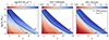 |
Fig. 1. Star formation rate and SFE adopted for the FFB model as a function of halo mass and redshift (Mv, z). Left: SFR. Middle: Instantaneous SFE |
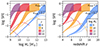 |
Fig. 2. Star formation efficiency adopted for the FFB model, as in Fig. 1, but via curves of SFE versus Mv for a given z (left) and SFE versus z for a given Mv (right). The SFE is made to coincide with the standard UM model (B19) (dashed lines) at low masses and redshifts and to approach ϵmax above the FFB thresholds of mass and redshift. The shaded areas refer to a maximum SFE that ranges from ϵmax = 0.2 (bottom) to 1 (top). The FFB threshold is at roughly 0.5 ϵmax. The SFE does not reach ϵmax for Mv ≥ 1012.5 M⊙ where SFR quenching is assumed. |
The FFB model predicts a strong redshift dependence in the SFE and the stellar-to-halo mass ratio following the evolving FFB threshold halo mass (Eq. (2)). A cautionary note that should be mentioned is that certain pre-JWST data (Stefanon et al. 2021) indicate only a weaker evolution of the SFE with redshift at z < 10.
3. Stellar masses, luminosities, and SFR density
3.1. Stellar mass function
The stellar mass function is given by
 (10)
(10)
where the conditional probability distribution in the first term is assumed to be a lognormal distribution with the median given by Eq. (7) and the standard deviation by Eq. (9), and n(Mv) is the halo mass function in the ΛCDM cosmology, adopted from Watson et al. (2013, with implementation by Diemer 2018) based on simulations that are reliable at z ∼ 10 and beyond (unlike most other similar work). The cumulative number density of galaxies with stellar mass above a threshold value is then N(> Ms) = ∫log Ms∞Φ(log Ms′) dlog Ms′.
Fig. 3 shows the predicted stellar mass function at z = 6–9, 12.5, and 16. As an alternative way to present the galaxy abundance, Fig. 4 addresses the stellar-mass distribution via the cumulative number density of galaxies with stellar mass above a threshold value, Ms > 109 M⊙ or 1010 M⊙, as a function of redshift4. The FFB predictions cover the range of ϵmax = 0.2 − 1 (areas between the orange and blue lines). They are compared to the standard UM model (B19) and the standard SAM (Yung et al. 2024a). The number density of 1010 M⊙ galaxies at z ≥ 8 predicted by the FFB model with ϵmax = 0.2 is 1dex higher than the standard models, and even more so at higher redshifts or when assuming a larger ϵmax. Also shown are the first observational results from JWST, tentatively indicating general consistency with the FFB model for massive galaxies at high redshifts for ϵmax ≳ 0.2.
 |
Fig. 3. Stellar mass function. Shown are the predictions of the FFB model at z = 6–9, 12.5, and 16. The blue and orange lines refer to ϵmax = 1 and 0.2, respectively. Shown for comparison are the extrapolated standard UM model (B19, solid gray line) and the results of a standard semi-analytic model (Yung et al. 2024a, solid dashed line). The FFB model predicts a greater abundance of massive galaxies, particularly evident from Ms ≳ 109 M⊙ at z ∼ 9. The excess for lower masses also becomes larger at higher z. The open symbols show pre-JWST observational constraints (Kikuchihara et al. 2020; Stefanon et al. 2021) and the filled symbols refer to tentative JWST constraints (Navarro-Carrera et al. 2024; Wang et al. 2024; Harvey et al. 2024; Weibel et al. 2024). The FFB predictions with ϵmax ∼ 0.2 seem to be consistent with the observed mass function at the massive end, though the evidence for deviations of the data from the standard UM model is only marginal for this statistic, especially at z ∼ 9. This is compared to the stronger evidence provided below by other observables. Indeed, we should note that SMF measurements suffer from large uncertainties in both observation and modeling. For example, assuming a bursty SFH (as expected by the FFB scenario, Sect. 4) rather than a smooth SFH during SED fitting results in an increased abundance of massive galaxies (gray squares; Harvey et al. 2024). |
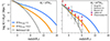 |
Fig. 4. Distribution of stellar masses. Shown are the FFB predictions for the number density of galaxies with stellar masses above 109 M⊙ (left panel) or 1010 M⊙ (right panel). The blue and orange lines refer to ϵmax = 1 and 0.2, respectively. The standard UM model (B19) is shown for comparison (gray line). The FFB predictions are above the UM model for z ≥ 6, and more so at higher redshifts. Shown for tentative comparison are the observational measurements compiled by Chworowsky et al. (2023), including JWST data (Labbé et al. 2023; Chworowsky et al. 2023) as well as earlier HST data (Song et al. 2016; Stefanon et al. 2021; Weaver et al. 2023). The JWST measurements are systematically higher than the previous measurements and they are above the standard UM model. The observations seem to favor the FFB prediction with ϵmax ≳ 0.2. |
The uncertainty in the estimates of stellar masses makes the comparison using the SMF as in Fig. 3 particularly tentative, as indicated by the big scatter among the different datasets, especially at z = 9. This is because the present stellar libraries, photoionization templates, and the wavelength range covered by the photometry are likely inadequate. For example, the inclusion of the mid-infra bands (MIRI) can make a significant difference in the stellar mass inferred from the spectral energy distributions (SED) (Papovich et al. 2023; Wang et al. 2024). We note that using a flexible bursty SFH in the SED fitting tends to yield more massive galaxies (Harvey et al. 2024), which makes the data agree better with the FFB model with ϵmax = 0.2. Despite the uncertainties concerning the SFHs of high-z galaxies (Tacchella et al. 2022b), certain studies suggested that allowing flexible nonparametric SFH may reproduce the true masses more reliably by accounting for outshining (Giménez-Arteaga et al. 2024; Narayanan et al. 2024). Theoretically, the FFB model indeed expects the high-z massive galaxies to have bursty SHFs (Sect. 4).
3.2. Luminosity function
The UV luminosity function (UVLF) is derived from the halo mass function as
 (11)
(11)
where MUV is the absolute UV magnitude (in the AB magnitude system). Here p(MUV|Mv), the probability distribution of the UV magnitude at a given halo mass and redshift, is assumed to be a Gaussian distribution. For the median, we adopt a simplified relation between the UV magnitude and the stellar mass obtained from stellar population synthesis in Yung et al. (2024a, Fig. 7)5,
 (12)
(12)
where Ms is taken from the median stellar-to-halo mass relation in Eq. (7), taking into account the enhanced luminosity in the FFB regime. The variance of {MUV|Mv} is assumed to be σMUV2 = 0.32 + (2.3σs)2, combining an intrinsic scatter of 0.3 mag in {MUV|Ms} (cf. Yung et al. 2024a, Fig. 7) and an uncertainty propagated from the scatter in the stellar-to-halo mass relation (Eq. (9)), 2.3σs, where the factor 2.3 comes from Eq. (12). We note that the high-luminosity end of the UVLF depends on the assumed variance (Shen et al. 2023).
The UV magnitudes can be corrected for dust attenuation AUV(Mv, z), by replacing median{MUV} with median{MUV}+AUV in Eq. (11). The attenuation of FFB and nonFFB galaxies are incorporated separately, using attenuation models from Sect. 8 and B19 (Eq. (23)), respectively.
Fig. 5 shows the FFB predicted UV luminosity function at z = 9–13 and 16, for ϵmax = 0.2 and 1. Shown are both the uncorrected LF and the LF corrected for dust attenuation based on Sect. 8. The LF from the FFB model is compared to the LF based on the standard UM model (B19), with and without their correction for dust. It is also compared to the LF in the standard SAM (Yung et al. 2024a) with no correction for dust. The FFB LF at the bright end is significantly higher than the standard predictions, more so at higher redshifts. For example, at z ∼ 12 the excess is higher by more than an order of magnitude already at MUV ∼ − 20. Current observational results from pre-JWST and from JWST are displayed on top of the theory predictions. While the scatter in the observational estimates is still large, the FFB model seems to provide a qualitative fit to the data, with an SFE that increases with redshift, e.g., indicating ϵmax = 0.2 − 0.5 at z ∼ 11.
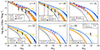 |
Fig. 5. Luminosity function. Shown are the FFB predictions for the rest-frame UVLFs of galaxies at z = 9–13 and 16. The colored bands represent dust-corrected FFB predictions for ϵmax = 0.2 (orange) or 1 (blue). The dust correction assumes either the shell or the disk version of the FFB model at the bottom or top bounds of the shaded area, respectively. The UVLFs uncorrected for dust are shown by dashed lines. Shown for comparison is the fiducial UM model (B19) (gray), corrected for dust (solid) or uncorrected (dashed). Also shown is the fiducial SAM simulation without dust attenuation (Yung et al. 2024a, dotted gray). The FFB predictions are well above the standard models, e.g., at z ∼ 9 for MUV ≥ − 19 and at z ∼ 12 for MUV ≥ − 18. The open gray data points are pre-JWST constraints (McLeod et al. 2016; Oesch et al. 2018; Morishita et al. 2018; Stefanon et al. 2019; Bowler et al. 2020; Bouwens et al. 2021; Harikane et al. 2022; Finkelstein et al. 2022a; only for z ≲ 10). The colored open symbols are measurements based on galaxies photometrically selected with JWST (Adams et al. 2024; Bouwens et al. 2023a,b; Castellano et al. 2022; Donnan et al. 2023; Finkelstein et al. 2022b; Harikane et al. 2023a; McLeod et al. 2024; Morishita & Stiavelli 2023; Naidu et al. 2022; Pérez-González et al. 2023; Yan et al. 2023; partly complied by Shen et al. 2023). In particular, bright-filled symbols are based on the JWST NGDEEP Epoch 1 (Leung et al. 2023, red), the complete CEERS sample (Finkelstein et al. 2023a, blue), and the JWST spectroscopically confirmed galaxies (Harikane et al. 2024, black). At z ∼ 11, the FFB predictions seem to match the tentative bright-end JWST observations with ϵmax ∼ 0.2 − 0.5. We note that the photometric constraints at z ∼ 16 are highly uncertain and possibly subject to redshift interlopers (Harikane et al. 2024). |
To highlight the excess of the luminosity function at high redshifts, Fig. 6 shows the redshift evolution of the UVLF at a given absolute magnitude, MUV = − 17 or −20. For example, at MUV ∼ − 20, the FFB LF is higher than the UM model by more than an order of magnitude already at z ∼ 10, and more so at higher redshifts. Current observational results from JWST are displayed on top. The fit of the FFB model to the data indicates ϵmax ∼ 0.2 at z = 8 − 12 and possibly higher efficiencies at higher redshifts.
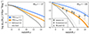 |
Fig. 6. Evolution of the UV luminosity function at MUV = − 17 (left) and −20 (right). Similar to Fig. 5, the colored bands represent dust-corrected FFB predictions for ϵmax = 0.2 (orange) or 1 (blue) and the gray line shows the fiducial UM model (B19). The UVLFs uncorrected for dust are shown by dashed lines. The FFB predictions at MUV = − 20 are higher than the UM model starting at z ∼ 7 and more so at higher redshifts. The open gray data points in the right panel are JWST measurements (Adams et al. 2024; Finkelstein et al. 2023a; McLeod et al. 2024). The tentative comparison indicates a fit with ϵmax ∼ 0.2 at z = 8 − 12 and possibly higher efficiencies at higher redshifts. |
Fig. 7 shows the FFB-predicted surface number density of galaxies above a given redshift for different magnitude limits. In order to compute this quantity, we converted the absolute magnitude MUV to the JWST apparent band mF277W using the luminosity distance and the K-correction. A linear relation is assumed between the rest-frame MUV and the observed-frame IR mF277W, whose slope and intercept are computed by fitting to a sample of galaxies in a semi-analytic model simulation (Yung et al. 2019a,b), in which spectral energy distributions (SEDs) were constructed based on the star-formation histories. A tentative comparison to observational results from the complete JWST CEERS sample (Finkelstein et al. 2023a) indicates consistency with the FFB model for ϵmax = 0.2 − 1. This is also consistent with the peak SFE estimated from the UVLF (e.g., Sun & Furlanetto 2016; Sipple & Lidz 2024).
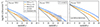 |
Fig. 7. Cumulative surface number density of galaxies. Shown is the surface number density per unit angular area at redshifts greater than z, for magnitude limits mF277W < 28.5, 29.5, and 31.5 in the three panels, respectively. The FFB predictions are for ϵmax = 1.0 (blue) and 0.2 (orange), with (solid) or without (dashed) dust correction. They are well above the standard UM predictions (gray). JWST observations are shown in the left and middle panels (gray shaded area), referring to the 68% confidence interval for z > 8.5 galaxies from CEERS (Finkelstein et al. 2023a) and NGDEEP (Leung et al. 2023) respectively. The horizontal dotted line indicates the surface density corresponding to one galaxy per JWST NIRCam field of view (9.7arcmin2). The tentative comparison indicates a fit with ϵmax = 0.2 − 1. Future JWST observations (e.g., DESTINY proposed for Cycle 3) can possibly reach down to mF277W ∼ 31.5. |
3.3. Evolution of the cosmic stellar mass and SFR densities
Given the stellar mass function from Eq. (10) and the luminosity function from Eq. (11), the cosmic density of stellar mass and UV luminosity are derived as functions of redshift,
 (13)
(13)
 (14)
(14)
where LUV is the luminosity corresponding to MUV. Similarly, the cosmic density of SFR can be estimated as
 (15)
(15)
where ⟨SFR|Mv, z⟩ is the mean SFR for a given halo mass and n(Mv|z) is the halo mass function (Watson et al. 2013). For comparison with observation, the above integrations are limited to galaxies brighter than MUV = − 17.5 or −17. In observation, ρUV is commonly used as a proxy for ρSFR, through ρSFR ≃ κUVρUV with a constant factor κUV ∼ 1.15 × 10⁻²⁸ M⊙ yr−1erg−1 s Hz that depends on the assumed initial mass function (IMF) and SFH (Madau & Dickinson 2014).
Fig. 8 shows the evolution with redshift of the average densities of stellar mass, UV luminosity, and SFR. The FFB model predictions are shown for the bounding values of ϵmax = 0.2 and 1. They are compared to the predictions of the standard UM model (B19), showing a significant over-density for z ≥ 8, which is growing with redshift. Current observational results from JWST are displayed on top of the predictions, indicating general consistency with the FFB model, tentatively indicating ϵmax ∼ 0.2. We note that the comparison between different densities and corresponding observations may each lead to a somewhat different result. This is partly because the different densities as derived from observations may involve different assumptions concerning quantities such as the IMF and the SFH, as well as the metallicity and dust obscuration, all affecting the conversion between SFR and UV emissivity.
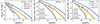 |
Fig. 8. Cosmological evolution of comoving densities. Left: Stellar mass. Middle: UV luminosity. Right: SFR. The densities are computed based on galaxies brighter than MUV = −17.5 or −17 as indicated in the labels. Shown are the FFB predictions for the bounding values of ϵmax = 0.2 and 1 (orange and blue respectively). Shown in comparison is the standard UM model (B19, gray). The shaded bands represent rough uncertainty estimates that correspond to varying the magnitude limits by 0.5 mag up or down. The FFB predictions are well above the UM model, starting with a small excess at z ∼ 8 and growing to an order of magnitude at z ∼ 12. Shown for tentative comparison are observational data (symbols). The FFB model seems to match the tentative data for UV and SFR density with ϵmax ∼ 0.2. The references include measurements of stellar density (Madau & Dickinson 2014; Papovich et al. 2023; Santini et al. 2023), UV density, and SFR density estimated from UV (McLeod et al. 2016; Oesch et al. 2018; Adams et al. 2023; Donnan et al. 2023; Harikane et al. 2023a; Pérez-González et al. 2023; McLeod et al. 2024; Finkelstein et al. 2023a; see also e.g., Coe et al. 2013; Ellis et al. 2013; Bouwens et al. 2020, 2023b,a; Robertson et al. 2023a). |
4. Star formation history
As discussed in Sect. 7 of D23, the main phase of star formation in an FFB galaxy is expected to last for a timescale comparable to the halo virial time  , which is at z ∼ 10 in the same ball park as the time for accretion of most of the baryons (Eqs. (31) and (32) there). This long phase is divided to Ngen ∼ 10 consecutive generations, each of a period tgen ∼ tvir/Ngen. Each generation starts with a peak episode that consists of FFB starbursts in many clusters and consumes gas fast. This peak episode lasts for a duration Δt of a few cloud free-fall times (∼ a few Myr) and is expected to be followed by a low-SFR period until the newly accumulated gas is sufficient for a new episode of fragmentation, bringing the onset of the next generation. The peak SFR is expected to be a factor tgen/Δt higher than the average SFR. Based on the accretion rate in Eq. (31) of D23, the latter is the SFE (ϵ) times the average baryonic accretion rate,
 (16)
(16)
The number of generations for the two extreme toy models of shells and disks that were considered in D23 are
 (17)
(17)
For disks this is based on the generation mass given in Eq. (60) of D23, assuming Q = 0.67, and the total mass fb Mv. For shells the generation mass is given in Eq. (46) of D23, with Rstr from Eq. (35), assuming T = 104 K and stream spin λs = 0.025, and with Rv from Eq. (23) there. At the threshold for FFB, Eq. (2), with n = 103.5 cm−3, this becomes
 (18)
(18)
Then, the period of each generation is
 (19)
(19)
At z ∼ 10, the generation period is thus expected to be on the order of 10 Myr, so we consider periods in the range tgen ≃ 5 − 20 Myr.
The peak duration reflects the spread in starburst time among the FFB clusters of a given generation. A lower limit would thus be the FFB time ∼1 Myr. An upper estimate could be the cloud-crushing time of a typical FFB cloud under the cumulative supernova wind from the clusters of earlier generations, which based on Eq. (17) of D23 is ∼5 Myr for a 106 M⊙ cluster. We therefore consider peak durations in the range Δt ≃ 2 − 5 Myr.
The SFH, with the two free parameters tgen and Δt, can be constrained by the distribution of the ratio of two different SFR indicators that are sensitive to different timescales, based on a sample of FFB galaxies. Here we use the SFR based on common SFR indicators such as Hα (or other Balmer lines) and FUV (1350–1750 Å), which are mostly sensitive to stars with ages of a few Myr and tens of Myr, respectively.
The upper panels of Fig. 9 show the toy model SFH for different choices of tgen and Δt and the associated Hα and FUV signals as a function of time. We note that the SFH as indicated by any Balmer line, such as Hα, Hβ, etc., is the same at first order (Tacchella et al. 2022a). The responses of the SFR using Balmer emission lines and FUV emission follow the approach in Caplar & Tacchella (2019). We predict the luminosity evolution for a Simple Stellar Population (SSP) using the Flexible Stellar Population Synthesis code (FSPS; Conroy et al. 2009; Conroy & Gunn 2010)6. We adopt the MILES stellar library and the MIST isochrones, with a metallicity of 0.1 Z⊙ for the stars and for the gas phase (without a qualitative effect on the results).
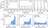 |
Fig. 9. Star formation history in an FFB galaxy at z ∼ 10. The intrinsic SFH consists of several generations, separated by tgen ∼ 10 Myr. Each generation consists of a peak of nearly simultaneous FFB starbursts that last for Δt = 2 − 5 Myr, followed by a quiet period of gas accumulation until the onset of the following generation of bursts. Shown are three cases where Δt = 2, 5 and tgen = 10, 20 Myr. Top: Simplified representation of the periodic bursty SFH (gray histogram) and as deduced from two different SFR indicators, using a Balmer line (Hα, Hβ, etc.; blue) or FUV (∼ 1500 Å; orange), which probe the SFR at different time-scales. Bottom: Distribution of the ratio between the SFRs as indicated by Balmer lines and by FUV for galaxies with SFH in the corresponding top panels. Quoted are the standard deviation and the skewness of the distribution, which can be used to constrain the characteristic Δt and tgen by observations. For a high duty cycle, Δt/tgen, the distribution is dominated by a single skewed peak at a ratio larger than unity, while a long quiet period tgen − Δt broadens the distribution toward ratios smaller than unity. This characteristic bursty SFH may bias the observed luminosities to even higher values at the bright end. |
As can be seen in the upper panels of Fig. 9, the Balmer peak height is suppressed and its width is extended compared to the intrinsic SFR peak, and these two effects are stronger for the FUV peak. The extension is because the photons are emitted from stars that live longer than the burst width. The duration for the Balmer lines is shorter because they require H-ionizing photons (λ < 912 Å) which are produced by massive short-lived stars, while the FUV photons are also produced by less massive, older stars. The bottom panels of Fig. 9 then show the corresponding distributions of the ratio log SFRBalmer/SFRUV, assuming that the galaxies are observed in a random phase of their periodic SFH. The distribution is narrow at a high ratio above unity when the duty cycle Δt/tgen is high. In all cases there is a peak at high SFRBalmer/SFRUV, corresponding to the early times within a generation when Hα is higher than FUV. If Δt/tgen is sufficiently low, and especially when tgen is high, at late times within a generation Hα drops to low values while FUV is still significant, leading to a second peak of the distribution at low SFRBalmer/SFRUV values. As illustrated by the numbers in the lower panels of Fig. 9, one can use two parameters to quantify the shape of the distribution, e.g., the overall standard deviation (σ) and the skewness (γ1). For example, while σ = 0.14 and γ1 = − 0.56 for the case (Δt, tgen) = (5, 10) Myr, they are σ = 0.44 and γ1 = 0.09 for (2, 20) Myr.
The SFH illustrated here is obviously oversimplified, and is meant for qualitative purposes. For example, the stochasticity in gas accretion can introduce an additional scatter of ∼0.3 dex (Dekel et al. 2013), which may dominate the variations in the SFH. More realistic predictions for the SFH variability will be obtained using cosmological simulations, semi-analytical or hydrodynamical. These will allow predictions for the temporal power spectrum of the SFH (e.g., Caplar & Tacchella 2019; Iyer et al. 2020; Tacchella et al. 2020) and the corresponding observable characteristics.
We recall that the bursty SFH, which is naturally predicted for the FFB phase, is likely to contribute to the enhanced luminosity function at the bright end, where the mass function is dropping steeply, causing low-mass galaxies to preferably scatter to high luminosities (Shen et al. 2023; Sun et al. 2023a,b). This will add to the main effect of enhanced SFE by FFB.
5. Steady wind and gas profile
An important element of an FFB galaxy is the outflowing wind driven by the cumulative supernova ejecta from the earlier generations of star clusters within the galaxy while the outer shell is forming new FFB star clusters. In D23 we crudely modeled this wind based on the mass in each generation of FFB, and used it to evaluate the condition for shielding of the new FFB clouds against crushing by this wind and for estimating the shell radius in balance between the forces exerted by the outflowing wind and the inflowing streams. Here, we model the wind somewhat differently as a steady wind that depends on the average SFR and the associated SFE and not explicitly on the generation mass, thus simplifying the expressions and reducing the dependence on free parameters. This leads to a prediction of the expected observed line width as a function of the SFE, and the steady-state gas density profile as functions of the SFE, SFR, and galaxy radius. We use this model in the following sections to re-evaluate the galaxy radius in the shell version of the FFB model, and to estimate the observable gas fraction, metallicity, and dust attenuation, all as functions of mass and redshift.
In the following analysis, we assume a constant SFE with the mean value as determined by the halo mass and redshift. As discussed in Sect. 4, FFB galaxies are expected to have bursty star formation histories with fluctuating SFE, which could influence the results presented below such as the estimates of the galaxy size and dust attenuation. For the purpose of the current qualitative estimates, we tentatively ignore these effects here and defer to future work the incorporation of the effects associated with the fluctuating SFE.
5.1. Steady wind
We consider the outflow generated by supernovae from a stellar system within a sphere of radius R, assuming here for simplicity a constant SFR during the ∼100 Myr formation time of the galaxy. The overall rates of mass and energy outflows (Ṁsn, Ėsn) increase over time as more stars explode in supernovae. The wind from each supernova is strong for about 20 Myr (see Figs. 1, 2 of D23). After such a period, the supernova outflow saturates in a steady wind with outflow rates that are determined by the SFR. Based on Leitherer et al. (1999), assuming Z ∼ 0.1 Z⊙, these outflows are
 (20)
(20)
We assume that the supernova ejecta loads additional interstellar gas into the wind, such that the mass outflow rate is related to SFR via a mass-loading factor η,
 (21)
(21)
The wind velocity is
 (22)
(22)
The mass-loading factor η can be expressed in terms of the SFE ϵ, defined here to be
 (23)
(23)
where Ṁin is the gas inflow rate onto the galaxy. Assuming that the inflowing gas that fails to be converted to stars constitutes the diffuse medium to be loaded onto the supernova wind, we write
 (24)
(24)
Using Eqs. (20), (21), (23) and (24), we obtain
 (25)
(25)
Based on Eq. (22) with Eq. (25), the wind velocity is predicted to be high and growing with the SFE, reflecting the associated dilution of the ISM,
 (26)
(26)
The observed line width at the wings is expected to be roughly FWHM ≃ 2 Vw, and the line may be split to two peaks symmetric about the zero velocity, depending on the actual geometry of the inflow and outflow. For high SFE in the FFB phase, where the ISM is rather dilute, these high supernova-driven velocities may be comparable to the velocities expected from AGN-driven winds (e.g., Kokorev et al. 2023; Harikane et al. 2023b). The FFB supernova-driven winds may be distinguishable by the associated lower metallicity (Sect. 7.2 below) and lower ionization, in terms of line ratios in the BPT diagram or electron densities (e.g., Kocevski et al. 2023; Maiolino et al. 2024). We note, however, that the line ratios may be quite different than usual in nonFFB star-forming galaxies or AGN due to excess emission from the supernova wind at > 70 eV (Sarkar et al. 2022). Being only a function of ϵ, the observed line width at the wings can be used to constrain the maximum SFE in the FFB phase with ϵ ≳ 0.2.
The potential effect of radiative losses on the wind is discussed in Sect. 8.4, where we find that they are expected to be ineffective at high SFE though they may slow down the wind for ϵ ≲ 0.2. The possible effect of galactic radiative-driven winds is discussed in Sect. 9.3.
5.2. Gas density profile
Given the outflow rates of mass and energy and the galaxy radius R, the steady wind has a mass density profile with different asymptotic forms interior and exterior to R (Chevalier & Clegg 1985),
 (27)
(27)
The gas density within the galaxy radius R is approximately constant. Inserting the outflow rates from Eq. (21), we obtain
 (28)
(28)
The discontinuity at r = R is due to a sharp transition from a subsonic wind within R to a supersonic wind outside, which in practice is materialized by a continuous steep drop near R.
6. Galaxy radius
The typical radii of FFB galaxies can be predicted as a function of mass and redshift in the two extreme cases of disks and shells, based on the estimate of D23 for disks and a slightly revised new estimate based on a steady wind for shells. Realistic galaxies might be mixtures of these two idealized cases.
6.1. Spherical shell model
The outflow comes to a halt when it encounters the inflow and creates a strong shock at a stalling radius Rsh, which can be associated with the galaxy boundary. The balance between the ram pressures of the outflow and inflow leads to
 (29)
(29)
where the first equality is based on Eq. (69) of D23 and the second equality is derived here based on the steady wind model, Sect. 5, replacing Eq. (70) of D23. Here Rstr is the effective radius of the streams, Ṁin = SFR/ϵ and Ṁout = η SFR are the inflow and outflow rates, Vw is the wind speed (Eq. (22)), Vin is the inflow stream speed, assumed to equal the virial velocity, Eq. (24) in D23. The factor  absorbs the dependence on ϵ, with f(ϵ) ≃ 1 for ϵ ≳ 0.2. Using the effective stream radius from Eq. (35) of D23, the shell radius becomes
 (30)
(30)
where λs, .025 ≡ λs/0.025 is the contraction factor of the stream width with respect to the width of the underlying dark-matter filament (Mandelker et al. 2018).
At the FFB threshold  from Eq. (2), we obtain
 (31)
(31)
The effective stellar radius may be very crudely assumed to be Re ≃ 0.5 Rsh, allowing a contraction to virialization by a factor of two.
We note that the shell radii obtained here using the steady wind model are only slightly different from those obtained based on Eq. (70) of D23. Both are determined specifically for the shell version of the FFB scenario.
6.2. Disk model
In the case of a disk, the typical gas disk radius is derived from the halo virial radius Rv and the contraction factor λ to be
 (32)
(32)
where  from Eq. (23) of D23. We note that this disk radius is generic, not special for the FFB scenario.
At the FFB threshold  , we obtain
 (33)
(33)
This radius may reflect the stellar effective radius of the disk.
One may crudely assume that the scatter in the size is dominated by the scatter in λ. If λ reflects the halo spin parameter, it is well fitted in ΛCDM cosmological simulations by a lognormal distribution with a dispersion σlnRe ∼ 0.5 in the natural logarithm (Bullock et al. 2001; Danovich et al. 2015; Yung et al. 2024b), though this has not been reliably examined for ∼1011 M⊙ halos at z ∼ 10.
In summary, based on Eqs. (30) and (32), we adopt for the galaxy radius (corresponding to ∼2Re) in the two toy models of shell and disk
 (34)
(34)
At the FFB threshold of Eq. (2), the associated galaxy radius as a function of redshift is
 (35)
(35)
While the radii in the two cases are comparable, the estimate for a shell is specific to the FFB model, while the estimate for a disk is rather generic to disk formation.
The predicted galaxy half-mass radius, Re (assumed to be = 0.5 R of Eq. (34)), is shown as a function of halo mass and redshift in Fig. 10 for the toy models of shell and disk with ϵ(Mv, z) computed as explained in Sect. 2.1. Also shown is the half-mass radius of typical galaxies at the FFB threshold of Eq. (2) as a function of z (Eq. (35)), in comparison with a collection of tentative JWST observational measurements. In order to focus on potential FFB galaxies, we display only the galaxies with an estimated stellar mass that is larger than 10% of the FFB threshold halo mass at the corresponding redshift.
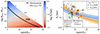 |
Fig. 10. Galaxy size. Left: Galaxy size as a function of halo mass and redshift as predicted by FFB disk model assuming an interim value of ϵmax = 0.5. Right: Predicted galaxy half-mass radius as a function of redshift for galaxies at the FFB threshold. The estimates by the two limiting FFB models of shell (blue) and disk (orange), from Eqs. (31) and (33), are pretty similar, predicting roughly |
7. Gas fraction and metalicity
7.1. Gas fraction
Integrating over the density profile from Eq. (28), the total gas mass in the galaxy is
 (36)
(36)
Inserting η(ϵ) from Eq. (25), SFR from Eq. (16), and R from Eq. (34), we obtain the gas mass Mg for the disk and shell models as a function of ϵ, Mv and z. Dividing Mg by the stellar mass Ms ≃ ϵ fb Mv, we obtain the mass ratio
 (37)
(37)
Here ϵ0.5 = ϵ/0.5, and η1.2 ≡ η/1.2 refers to ϵ = 0.5. For ϵ = 1 or 0.2, η = 0.2 or 4.2 respectively, so the ratio should be multiplied by ∼0.06 or 6 respectively. At the FFB threshold given in Eq. (2), we obtain as a function of redshift
 (38)
(38)
When this ratio is small it is a proxy for the gas fraction, fgas = Mg/(Mg + Ms).
Fig. 11 shows the gas fraction as a function of redshift at the FFB threshold for the shell and disk models. It is predicted to be rather low, fg < 0.1 for ϵ > 0.2. A higher SFE leads to a smaller fg due to its dependence on η in Eq. (38), reflecting the smaller amount of residual gas left after star formation.
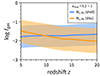 |
Fig. 11. Gas fraction. Shown is fgas = Mg/(Mg + Ms) within R ≃ 2Re as a function of redshift at the FFB threshold, based on Eq. (38), for ϵmax = 0.5 in the shell and disk models. The shaded bands indicate the uncertainty due to ϵmax ranging from 0.2 (top) to 1 (bottom). The gas fraction is rather low in the whole FFB regime, largely due to the low mass-loading factor associated with the high SFE. |
7.2. Metallicity
Based on their Fig. 1, showing the Starburst99 mechanical energy injection rate of stellar winds from a 106 M⊙ starburst, D23 expressed the worry that the winds may suppress the SFR if the metallicity in the star-forming clouds is Z ≥ 0.2 Z⊙. On the other hand, the simulations of Lancaster et al. (2021) indicated that mixing and cooling at the interface of the hot bubble and the cold ISM are likely to make the stellar winds ineffective for a few free-fall times even when the metallicity is as high as solar. Even if this conclusion is not valid under all circumstances, one can argue that the stellar winds should not be disruptive because, as we show here, the metallicity in the FFB star-forming clouds is expected to be low. The worry is that metals carried by supernova winds from the earlier generations of stars in the galaxy may contaminate the clouds in the outer shell or ring where the FFBs are expected to occur. This is unlikely for two reasons. First, the mixing of the metals in the clouds is expected to occur on a Kelvin-Helmholtz timescale. As evaluated in Sect. 4 of D23 in the context of the cloud shielding against the supernova-driven wind, this timescale is expected to be longer than the cloud free-fall time once the clouds are more massive than ∼104 M⊙. Second, we show below that even in the event of full mixing, the metallicity in the clouds is expected to remain relatively low, at the level of Z ∼ 0.1 Z⊙.
Assuming that the FFB clouds in the shell are limited to the areas of the shell that come into direct contact with the inflowing streams, only a fraction of the outflowing metals participates in the mixing, fΩ ≡ Ωstr/4π, where Ωstr is the solid angle corresponding to the streams. According to Eq. (29), we have
 (39)
(39)
where  for ϵ ≳ 0.2. This gives in the FFB regime fΩ ∼ 0.2 rather insensitively to the value of ϵ.
The mass of gas that outflows into the stream-fed regions of the shell (denoted by ′) is
![Mathematical equation: $$ \begin{aligned} \dot{M}{\prime }_{\rm out} = f_\Omega \, \dot{M}_{\rm out} = f_\Omega [\dot{M}_{\rm sn} + (1 - \epsilon ) \dot{M}_{\rm in}], \end{aligned} $$](/articles/aa/full_html/2024/10/aa48727-23/aa48727-23-eq49.gif) (40)
(40)
(cf. Eq. (24)). Similarly, the outflow rate of metal mass into these areas is
![Mathematical equation: $$ \begin{aligned} \dot{M}{\prime }_{{\mathrm{out} }, Z} = f_{\Omega }\, [\dot{M}_{{\mathrm{sn} }} Z_{{\mathrm{sn} }} + (1 - \epsilon ) \dot{M}_{{\mathrm{in} }} Z_{{\mathrm{in} }}], \end{aligned} $$](/articles/aa/full_html/2024/10/aa48727-23/aa48727-23-eq50.gif) (41)
(41)
The first term represents the metals ejected by the supernovae, with  (see Eq. (20)) and metalicity Zsn. The second term represents the gas that came in by inflow, with metallicity Zin, and has not turned into stars.
The outflowing metals and mass are assumed here to mix with the inflows, Ṁin,Z = Ṁin,Zin. The mixed metallicity is then
 (42)
(42)
Fig. 12 shows the mixed metallicity as a function of redshift at the FFB threshold of Eq. (2), assuming Zsn ∼ 1 Z⊙ and Zin ∼ 0.1 Z⊙ for ϵmax = 0.2 − 1. The mixed metallicity is in the ball park of Zmix ∼ 0.1 Z⊙ at all redshifts, indicating that the enrichment by outflow is rather weak (because of the low fΩ of penetrating cold streams) and quite insensitive to redshift or ϵmax. This is a conservative upper limit for the metallicity in the FFB clouds. The metallicity becomes even lower when assuming lower metallicity in the accreted gas, e.g., Zin = 0.02 Z⊙. Shown for comparison are tentative JWST observational measurements, which indicate low but non-negligible metallicities in the ball park of the model predictions.
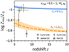 |
Fig. 12. Metallicity. Shown is the upper limit for the metalicity in FFB star-forming clouds, assuming full mixing between the outflowing metals Zsn = 1 Z⊙ and inflowing gas Zin = 0.1 Z⊙ (blue) or 0.02 Z⊙ (orange) in Eq. (42). The metalicity is computed for halos at the FFB threshold mass. The bottom and top bounds of the shaded areas represent ϵmax = 0.2 and unity, respectively. Despite the mixing with supernova-enriched gas from earlier generations, the metallicity remains low and close to Zin, at Z ∼ 0.1 Z⊙ or below. Shown for reference are tentative observations (Curti et al. 2023, 2024; Jones et al. 2023; Hu et al. 2024; also cf. Arellano-Córdova et al. 2022), which suggest low but not negligible metalicities in the same ball park, though these galaxies are not necessarily in the FFB regime. |
We conclude that as long as the observed gas metallicity is dominated by the gas in the FFB star-forming clouds, from which most of the UV luminosity is emitted, the predicted gas metallicity to be observed in a galaxy during its FFB phase is in the ball park of Z ∼ 0.1 Z⊙. This is high enough for the cooling time to be shorter than the free-fall time, as required for a burst at the FFB densities, and, in turn, it is low enough to guarantee that the stellar winds are not suppressing the FFB.
8. Dust attenuation
8.1. Attenuation at a given SFR
Here, we use the global steady-wind model of an FFB galaxy to estimate its expected dust attenuation as a function of halo mass and redshift. The results are to be used to correct the predicted observable luminosities in the FFB regime, e.g., in the luminosity function.
Integrating over ρ(r) in Eq. (28) along a radial line of sight in the two regimes inside and outside the galaxy, we obtain the column density of Hydrogen atoms,
 (43)
(43)
where the first and second terms refer to integration over r < R and r > R respectively.
Given NH, the optical depth at 1500 Å is
 (44)
(44)
where σext, mw ≃ 10−21 cm2/H is the corresponding extinction cross section of the dust per H nucleon in the Milky Way (Weingartner & Draine 2001) and fd is the dust-to-gas ratio in the outflow with respect to its value in the Milky Way. The factor fd in principle has contributions both from the supernovae (fd, sn) and from the inflowing gas. For low metallicity in the inflow, Zin ≪ Z⊙, relevant for FFB, the contribution from the inflow turns out to be negligible (see Sect. 8.3), such that
 (45)
(45)
with fd, sn = 5 − 8 ≃ 6.5 for Z ∼ 0.1 Z⊙ in stars (Marassi et al. 2019). Inserting NH from Eq. (43) in Eq. (44) we obtain
 (46)
(46)
The corresponding obscured fraction is determined from the optical depth as fobsc = 1 − e−τ. The attenuation in UV is
 (47)
(47)
Assuming that the new FFB star formation occurs mostly in a shell or a ring near R, such that the luminosity originates mostly there, the more relevant obscuration is by dust at r > R. In the shell toy model, one could very crudely assume that half the shell closer to the observer is obscured only by the dust in r > R, while the other half is obscured by the dust in r > 0, such that the effective obscured fraction is the average of fobsc, r > R and fobsc, r > 0. In the case of a ring in the outskirts of a disk, for a line-of-sight that does not lie near the disk plane, the effective obscuration may be very crudely estimated by fobsc, r > R alone. For example, for ϵ = 0.5, SFR = 65 M⊙ yr−1 and R = 0.5 kpc, we estimate fobsc in the ball park of 0.6 − 0.8.
8.2. Attenuation in the FFB regime
We can further express τ as a function of ϵ, Mv and z. The average SFR, based on Eq. (31) of D23, is given by Eq. (16). Using the galaxy radius from Eq. (34) for the two toy models of shell and disk adopting a contraction factor λ.025 = 1, and inserting these SFR and R in Eq. (46), we obtain
 (48)
(48)
where  . For the disk model we only consider r > R, while for the shell model we adopt the average fobsc in the ranges r > 0 and r > R, resulting in an effective prefactor of 0.36 for disks and 0.99 for shells in Eq. (48). Interestingly, the dependence of τ on the SFE ϵ is rather weak when ϵ ≳ 0.2, with f(ϵ) = 1, 1.22, 0.92 for ϵ = 1, 0.5, 0.2 respectively. This is because the increase of SFR with ϵ is roughly balanced by the decrease of η with ϵ.
At the FFB threshold as estimated in Eq. (2), we obtain in Eq. (48)
 (49)
(49)
Fig. 13 shows the obscured fraction as a function of redshift, based on Eq. (49) with ϵmax = 0.5, valid for Zin ≪ 1 (solid lines). The shell and disk toy models are compared. We see a significant decline of fobsc with redshift for typical galaxies at the FFB threshold. The tentative JWST observational measurements seem to lie between the FFB predictions for shells and disks, though they do not necessarily correspond to FFB galaxies. The model predictions are also consistent with the low dust suggested by the very blue UV slopes for high-z galaxies (Topping et al. 2024; Morales et al. 2024).
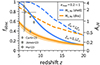 |
Fig. 13. Obscured fraction fobsc = 1 − e−τ as a function of redshift z along the threshold line for FFB, according to Eq. (49). The corresponding extinction AUV is shown on the right y-axis. The toy models of the shell (blue) and disk (orange) are shown, with similar results. The color bands show the uncertainty corresponding to ϵmax = 0.2 − 1 about ϵmax = 0.5. We see a significant decline in obscuration with redshift. The solid lines are for Zin = 0.1, typical in the FFB regime. Shown for comparison (dashed line) are the results for Zin = 1, valid at later times, where the obscuration is stronger. Shown for reference are tentative observations (Curti et al. 2023; Jones et al. 2023; Hu et al. 2024; assuming a Calzetti et al. 2000 attenuation law), which lie between the FFB predictions for shells and disks. |
8.3. Attenuation at low redshift and high metallicity
For completeness, we comment that at lower redshifts, away from the FFB regime, when Zin (in solar units) is not much smaller than unity, the inflowing gas can make fd grow significantly, and thus increase τ1500. To see this, define δ to be the dust-to-gas ratio in the different components. Based on Rémy-Ruyer et al. (2014), δ in the inflowing gas is found empirically to be
 (50)
(50)
where δmw is the ratio at solar metallicity, assumed to be valid in the ISM of the Milky Way. By definition, fd = δout/δmw, where δout = Ṁdust/Ṁout. For the dust we write
 (51)
(51)
Using δsn = fd, sn δmw based on the definition of fd, sn, as well as Eqs. (23) and (50), we get
 (52)
(52)
Inserting Ṁdust in δout = Ṁdust/Ṁout, and using Eqs. (20) and (21), we finally obtain
![Mathematical equation: $$ \begin{aligned} f_{\rm d} = \frac{\dot{M}_{\rm dust}}{\dot{M}_{\rm out}\delta _{\rm mw}} = \eta ^{-1}\, [0.2f_{\rm d,sn} + (\epsilon ^{-1}-1)\, Z_{\rm in}^{1.6}]. \end{aligned} $$](/articles/aa/full_html/2024/10/aa48727-23/aa48727-23-eq64.gif) (53)
(53)
The second term is indeed negligible for Zin ∼ 0.1 Z⊙, namely in FFB conditions, but it dominates if Zin ∼ Z⊙ and ϵ ≪ 1, valid at low redshifts. The obscured fraction for Zin = Z⊙ is also shown in Fig. 13 for comparison.
8.4. The effect of cooling in the wind
The analysis so far neglected the possible effect of radiative cooling of the wind within the galaxy, which could, in principle, weaken the outflow and enhance the dust attenuation if the effective cooling radius rcool is smaller than the galaxy radius R. Eq. (6) of Thompson et al. (2016) provides an estimate of the cooling radius in terms of the galaxy radius,
 (54)
(54)
where η = ϵ−1 − 0.8 is the mass loading factor (Eq. (25)), R0.3 = R/0.3 kpc and SFR10 = SFR/(10 M⊙ yr−1). For a crude estimate, we insert the galaxy radius in the shell model from Eq. (30) and the SFR from Eq. (16) in Eq. (54) to obtain
 (55)
(55)
This ratio also scales with  , which we assume here to equal unity. For the halos of the FFB threshold mass
  , this ratio becomes
 (56)
(56)
We learn that for the high values of SFE and z that are relevant for most of the FFB regime, the cooling radius is larger than the galaxy radius, so the correction for cooling is small. Cooling may become marginally effective at low ϵ or low z. For example, according to Eq. (56), at (1 + z) = 10, rcool ∼ R for ϵ < 0.23, namely cooling may be important at the low bound of the FFB regime. At z ≳ 11, on the other hand, rcool > R even for ϵ = 0.2, so cooling is unimportant in the whole range of SFE that is relevant for FFB. In the nonFFB regime, where ϵ ≪ 1, rcool drops below R due to the strong ϵ dependence in Eq. (56). When rcool ≤ R, the wind terminates at r < R inside the galaxy, so the gas and dust are confined to radii smaller than R. In this case, if the star formation is mostly in an outer shell or a ring of radius R, the obscured fraction is expected to be in the range 0–0.5 for ring or shell respectively, implying that less than half of the light from the star-forming region is obscured. This is actually comparable to the result for a wind with no cooling.
There are several additional factors that can suppress the radiative cooling in the wind beyond the cooling rate that led to Eq. (54). First, Sarkar et al. (2022) showed that the cooling can be suppressed by nonequilibrium ionization in the wind and by excess radiation produced by the hot gas in the star-forming region. Second, entropy can be regenerated in the hot wind by bow shocks created at the interface between the wind and cold clouds (Conroy et al. 2015; Nguyen & Thompson 2021; Fielding & Bryan 2022), though it is possible that mixing of cold and hot gas near these clouds may overwhelm this increase in entropy. Based on all the above, we can conclude that the estimates of gas fraction, metallicity, and dust attenuation that neglected cooling in the wind are viable approximations in the FFB regime.
9. Discussion
9.1. Additional mechanisms for bright galaxy excess
Beyond the enhanced SFE due to FFBs presented in D23 and discussed here, there are several additional mechanisms that can potentially contribute to the excess of bright galaxies at cosmic dawn compared to extrapolations of the standard model and current simulations. Four different general types of additional mechanisms come to mind as follows.
-
Scatter in the luminosity at a given halo mass, e.g., due to burstiness in the star-formation rate, which preferentially scatters low-mass halos to higher masses at the massive end, where the halo mass function is declining steeply (Sun et al. 2023b; Yung et al. 2024a).
-
Enhanced ratio of UV luminosity to stellar mass, e.g., by a top-heavy IMF, or by a nonstellar UV source such as AGN (Yung et al. 2024a; Tacchella et al. 2023b; Grudić & Hopkins 2023).
-
Reduction in dust attenuation at higher redshifts (Ferrara et al. 2023; Ferrara 2024).
-
Modifications of the standard ΛCDM cosmology that are associated with an enhancement in the abundance of massive halos, such as the introduction of Early Dark Energy (Klypin et al. 2021) or enhanced primordial power spectrum (Parashari & Laha 2023).
The enhanced SFE is robustly predicted by the physical model of FFB, which is naturally expected preferentially at the high densities and low metallicities present in high-mass halos at cosmic dawn. This mechanism alone can enhance the observed luminosities by an order of magnitude. As shown in Sect. 4, the FFB scenario naturally involves a characteristic bursty SFH at the bright end, which could bias the luminosity further to higher values. Furthermore, as estimated in Sect. 8, the dust attenuation in the FFB regime is expected to be low and to decrease further with redshift, which also helps to make the galaxies brighter.
The consideration of a nonstandard IMF is currently under both theoretical and observational uncertainties, potentially either suppressing or enhancing the FFB mechanism and the abundance of early bright galaxies (see a more detailed discussion in Sect. 9.2). The involvement of AGN in enhancing the UV luminosity is also conceivable but remains rather uncertain and yet to be explored; tentative indications suggest that the contribution of AGN to the UV at cosmic dawn is subdominant (Scholtz et al. 2023). Finally, turning to modifications of ΛCDM would necessarily involve ad hoc free parameters, potentially conflicting with the spirit of the simplicity principle of Occam’s razor.
Overall, it is important to come up with observable features that could constrain the contribution of each mechanism to the excess of bright galaxies. The main observable distinguishing feature of the FFB scenario is the preferred appearance of high SFE at high redshifts and possibly at high halo masses. Such a mass dependence does not seem to emerge as a natural intrinsic feature if a top-heavy IMF is responsible for the bright excess, or if variations in dust attenuation are responsible for the redshift dependence of the excess (see Finkelstein et al. 2023a).
9.2. Initial mass function
The IMF at cosmic dawn is unknown. Given both the theoretical and observational uncertainties, it could deviate from the standard low-redshift IMF either way, towards a top-heavy or a bottom-heavy distribution. Such deviations could either suppress or enhance the FFB nature of galaxy formation and the excess of early bright galaxies.
On one hand, there are observational indications that the stellar populations in the cores of massive elliptical galaxies at low redshifts have a bottom-heavy IMF (Conroy & van Dokkum 2012; van Dokkum et al. 2017; Hallakoun & Maoz 2021). If these are the descendants of the early FFB galaxies, in agreement with the average halo mass growth of three orders of magnitude from z ∼ 10 to the present, it would indicate that the FFB population had a bottom-heavy IMF. In agreement, simulations that include radiative and proto-stellar outflow feedback find that these processes tend to induce an IMF with a lower characteristic stellar mass and an overall narrower mass range in high surface density environments (Tanvir et al. 2022), typical of the star-forming clouds at cosmic dawn. When the IMF is bottom-heavy, the deficiency in OB stars would lead to suppressed supernova and stellar feedback, enhancing the FFB nature of galaxy formation at cosmic dawn even beyond the direct primary effects of high densities.
On the other hand, a top-heavy IMF may be expected at cosmic dawn due to the high cosmic microwave background (CMB) temperature or the high ISM pressure and density, as indicated in other simulations (Grudić & Hopkins 2023; Bate 2023; Yung et al. 2024a). A top-heavy IMF is also indicated under certain assumptions from observations, e.g., in two nebular-dominated galaxies at z ∼ 6 − 8 (Cameron et al. 2023) or by fitting the photometry of high-redshift galaxies with revised templates (Steinhardt et al. 2023). By enhancing the UV luminosity-to-mass ratio, a top-heavy IMF could contribute to an increased abundance of bright galaxies. However, typical simulations indicate only a limited factor of 2–3 in luminosity enhancement (Yung et al. 2024a), which may not be sufficient by itself to explain the full excess of bright galaxies. Furthermore, the excessive radiation pressure associated with a top-heavy IMF will tend to suppress the SFE and thus act to reduce the excess of bright galaxies, leaving the net effect uncertain. Simulations by Menon et al. (in prep.) find that a top-heavy IMF with a luminosity-to-mass ratio that is larger by an order of magnitude than the standard could reduce the SFE by a factor of two, but the suppression is smaller at the low metallicities and dust content expected at cosmic dawn, where the radiative feedback in high-surface-density clouds is largely by IR radiation pressure on dust. This indicates that a top-heavy IMF and a high SFE can co-exist.
In parallel, a top-heavy IMF can generate FFB in an alternative way, by accelerating the core collapse to black holes at the centers of the star-forming clusters (Dekel et al., in prep.). This process is driven by the inward migration of the massive stars due to dynamical friction, which would be naturally enhanced when more massive stars are present (Portegies Zwart & McMillan 2002; Rizzuto et al. 2023). The core collapse of clusters is further sped up by the rotation and flattening of the clusters that form in galactic disks (Ceverino et al. 2012), via a process of gravo-gyro instability (Hachisu 1979; Kamlah et al. 2022). In clouds where this core collapse occurs within a few Myr, it is expected to eliminate the massive stars before they can generate effective feedback at the end of their lifetimes, thereby leading to FFB. From the above discussion, we conclude that the IMF at cosmic dawn and its implications on FFB and the excess of bright galaxies remain largely uncertain, necessitating more thorough exploration.
9.3. Radiatively driven versus supernova-driven wind
The analysis of gas fraction, metallicity and dust in Sects. 7 and 8 is based on an assumed supernova-driven wind in steady state, as presented in Sect. 5. This wind is assumed to be driven by supernovae from earlier generations of stars, in their active supernovae phase, during most of the ∼100 Myr duration of the FFB galaxy formation phase. Here we comment on the validity of this supernova-driven wind in view of a possible global gas (and dust) ejection from the galaxy by super-Eddington radiative-driven winds, as proposed by Ferrara (2024). Based on Eq. (2) of Ferrara (2024), super-Eddington ejection is expected to occur once the specific SFR in the galaxy is above a threshold,
 (57)
(57)
Here A is the ratio of dust to Thomson scattering cross-section and fbol is the bolometric correction with respect to the UV luminosity at 1500 Å, both set to their fiducial values. We introduce the correction factor fts, the ratio of total to stellar mass within the galaxy, to account for the neglected contribution of the nonstellar mass to the Eddington luminosity. With a gas-to-stellar mass ratio of ∼0.5 and a moderate additional contribution of dark matter one can assume fts ∼ 2. However, this factor may be balanced by a larger value of A, so we conservatively ignore it.
Ferrara (2024) assumes that the radiation dominates over the supernovae in driving the wind. Tentatively adopting this hypothesis, we evaluate the redshift range of validity of the condition in Eq. (57). Based on Dekel et al. (2013), the analytic estimate in their Eq. (7) and their simulation results, we approximate the sSFR by the specific accretion rate onto the halo,
 (58)
(58)
This redshift dependence is consistent with the findings of Zhao et al. (2009) and it has been shown to be a better and more physical approximation than the crude estimate that is used by Ferrara (2024) based on the ratio of halo mass to halo crossing time (see the difference between eqs. (31) and (32) of D23). Inserting the sSFR from Eq. (58) in Eq. (57), one expects super-Eddington ejection at
 (59)
(59)
Assuming the fiducial values of the parameters, this implies a conservative lower limit of zcrit ≃ 16 for halos of Mv ∼ 1011 M⊙. If we adopt the weak mass dependence in Eq. (58), and insert the declining Mv, ffb(z) at the FFB threshold from Eq. (2), we can solve Eq. (59) for z to obtain zcrit ≃ 22. The value of zcrit = 16, and certainly zcrit = 22, are beyond the redshift range of the current JWST observations in which the excess of bright galaxies is detected, making the radiative-driven global winds less relevant for the main FFB phase.
At these extremely high redshifts when super-Eddington winds prevail, we return to the question of whether it is justified to neglect the SN-driven winds in the first place. A quick comparison with the equivalent pressure produced by the SNe and radiation shows that these pressures are almost equivalent (Thompson et al. 2005; Murray et al. 2011). However, the SNe-driven pressure may be reduced due to radiative cooling such that the SNe pressure becomes much lower, and an energy-driven solution may not be viable for individual SNe. In such cases, the common wisdom is that a momentum-driven wind dominates. Even in this case, it is found that the wind-driving forces exerted by supernovae and by radiation from stars are comparable, at ṗ/m∗ ∼ 6 × 10⁻⁸ cm s−2 (Grudić et al. 2020), and both are comparable to the additional contribution from stellar winds. We recall that the momenta from clustered sources, as expected in particular in the FFB compact clouds in compact galaxies at z ∼ 10, add up super-linearly for supernovae (Gentry et al. 2017), but linearly for radiative pressure, making the supernovae more important. At significantly clustered star formation regions (as is the case for the high redshift galaxies under consideration), the wind becomes energy-driven again. Such highly clustered SNe can retain 20–100% of the SNe energy (Fielding et al. 2018), as estimated observationally in M82 (Strickland & Heckman 2009).
Furthermore, the pre-blast wave energy losses of SN bubbles due to their interaction with the ISM, highlighted in Ferrara (2024), are relevant only when the ISM is dense (≳105mp cm−3; Terlevich et al. 1992), as it is in the first free-fall times of the first starbursts, prior to the onset of effective SN feedback. Soon after, the ISM becomes dilute (in gas density, metals and dust) due to both the high SFE of conversion of gas into stars and the super-Eddington winds. The SN-driven steady wind (Sect. 5) keeps the ISM dilute for the rest of the ∼100 Myr global FFB phase (Sect. 7). In such a dilute ISM, the radiation-driven wind is expected to become negligible, as there is only little dust to respond to the radiation pressure. In turn, the dilute ISM allows the SN-driven wind stream freely and be as effective as it could. In more detail, there could be repeating episodes of a dense ISM (dusty and red) followed by a dilute ISM (dust-free and blue) in a characteristic duty cycle, as eluded to in Ferrara (2024). This is as predicted in our FFB scenario, Sect. 4 and D23. During the dense episodes, one may expect bursty super-Eddington ejection on top of the steady SN-driven wind, but typically only at the very high redshifts indicated by Eq. (59).
We conclude that super-Eddington ejections are potentially valid only at very high redshifts beyond the current main observed range, and even when they are, they are not likely to overwhelm the steady supernova winds that we use as a basis for our estimates of gas fraction, metallicity and dust attenuation. Nevertheless, based on the SN-driven winds, we do predict low dust attenuation at high redshifts, which becomes negligible at very high redshifts, where it is also predicted to be removed in episodes of super-Eddington winds.
While Ferrara (2024) argues that being dust-free is enough to bring the observed luminosities and SFRs to the level of the JWST observations, this is not the case in massive halos at cosmic dawn based on the tentative comparisons shown in figures above between JWST observations and the standard nonFFB models; for example, as represented by the UM empirical model (B19) naively extrapolated to high redshifts and the standard SAM (Yung et al. 2024a), both with no dust correction. Being dust-poor may help, especially at very high redshifts, but the main contribution to the excess of bright galaxies and high SFR at cosmic dawn is likely to be the enhanced SFE because of FFB, helped by the associated bursty SFE, maybe by a somewhat top-heavy IMF, and possibly by UV from AGN.
9.4. Choice of “standard” UM model
A word of caution is called for concerning the use of the empirical UM model (B19). We used it to normalize the SFE at low redshifts and low masses away from the FFB regime. Then, in certain occasions, we compared our predictions for FFB with extrapolations of the UM model to the relevant high redshifts. One should be aware of the fact that the current version of the UM model has been derived based on observations at lower redshifts, and the results with which we were comparing are based on uncertain extrapolations to z ∼ 10. These “predictions” of the UM at high redshifts should therefore be considered with a grain of salt. This uncertainty in the UM model does not affect our predictions in the FFB regime, in which the UM predictions are not involved. The UM can eventually be revised to refer to z ∼ 10 by fitting the model to new JWST observations and thus recover the excess of bright galaxies at high redshifts.
9.5. FFB at lower redshifts
In principle, the FFB phenomenon may occur and be observable at redshifts and/or masses below the FFB threshold of Eq. (2), with decreasing abundance further below the threshold line. These FFBs can naturally arise in our simple FFB model from the scatter in the parameters that control the density in the star-forming regions, which, once in the tails of their distributions, may bring the density to above the required threshold for FFB. For example, this may occur in disks of particularly small sizes that derive from small values of λ, or where the gas inflows are denser and/or more supersonic than the average for the given halo mass. Alternatively, different mechanisms, such as wet galaxy mergers, intense instreaming, or other compaction events, may drive the required high densities and generate starbursts with high SFEs even at later times (Krumholz et al. 2012; Zolotov et al. 2015; Turner et al. 2015; Lee et al. 2016; Usero et al. 2015; Fisher et al. 2022; Querejeta et al. 2019; Lapiner et al. 2023). These later high-SFE starbursts, however, may not necessarily follow the “standard” FFB scenario worked out above and may therefore not share all the properties that were predicted for high-z FFB galaxies.
Densities above the FFB threshold of ncrit ∼ 3 × 103 cm−3 apparently appear in dense regions within giant molecular clouds (GMCs) in low-redshift disk galaxies. However, contrary to the FFB clouds, the GMCs are believed to have low overall SFEs that are likely suppressed by feedback, which actually tends to disrupt the clouds in a few dynamical times (e.g., Krumholz 2017). Two obvious distinguishing features between GMCs and high-z FFBs are the metallicity and the background disk density. The metallicity is near solar in GMCs while it is well below solar in FFBs, and the background disk density is much lower than the FFB density in GMCs while it is not far below the FFB density in FFBs. In GMCs, the low disk density makes the cloud contraction (either at the original cloud formation or at its reformation after disruption) be slow, on the disk free-fall timescale, which is longer than the ∼1 Myr time window for FFB. During this contraction, the high metallicity makes tcool < tff already in the early phases of cloud contraction, allowing star formation to occur before the cloud develops the dense core, thus leaving no time window free of supernova feedback. In FFBs, on the other hand, the high disk density makes the collapse rapid, on a cloud free-fall timescale of ∼1 Myr, and the low metallicity makes the cooling time drop below the free fall time and allow star formation only once the density exceeds the critical FFB density. This permits a burst free of feedback.
Furthermore, based on measurements of HCN/CO ratio, the regions in GMCs where the density is above ncrit, which tend to be filamentary structures, are estimated to occupy only ∼10−3 of the GMC volume in local disks, with a clear trend upwards with larger galactic-averaged density (Mark Krumholz, private communication; based on, e.g., Jiménez-Donaire et al. 2019). This makes the surface density in local GMCs of size < 100 pc lower than the critical surface density of Σcrit ∼ 3000 M⊙ pc−2 required for preventing significant gas ejection by stellar radiation pressure (Menon et al. 2023), but probably not so in high-redshift FFB clouds that reside in much denser background disks. Therefore, the SFR in local GMCs is not expected to be free of radiative feedback the way the high-z clouds are.
10. Conclusion
As proposed analytically by D23, feedback-free starbursts (FFB) are expected in gas clouds where the gas density exceeds a critical value of n ∼ 3 × 103 cm−3. This ensures that the free-fall time is ≤1 Myr, which is shorter than the timescale for feedback from supernovae and stellar winds, and also ensures that the cooling time is shorter than the free-fall time, allowing a starburst to occur on a free-fall timescale. Moreover, the gas surface density in the FFB clouds should be above Σ ∼ 2 × 10³ M⊙ pc−2 to guarantee that radiative feedback is ineffective.
Consequently, enhanced SFE, of namely SFE ∼ 0.2 − 1, is expected in halos above a threshold in mass and redshift, roughly defined by the curve  , leading to distinguishable observable predictions, as follows.
-
The average cosmological SFR density should be enhanced compared to the “standard” low-SFE scenario – a small overdensity at z ∼ 8 and a large overdensity at z ∼ 12.
-
The galaxy mass and luminosity functions are expected to be correspondingly enhanced at z ≥ 8, and gradually more so at higher masses and brighter magnitudes. For example, at z ∼ 12, galaxies of UV magnitudes of −20 are expected to be overabundant by more than an order of magnitude compared to the extrapolated standard empirical model of low SFE (B19).
-
The SFH, during the global galaxy formation time of ∼100 Myr, is expected to be bursty on a timescale of ∼10 Myr. In each such generation, a peak in SFR is expected to be followed by a low-SFR phase. This duty cycle should be translated to a global average SFE that is smaller than unity, possibly as small as 0.2. The predicted bursty SFH should be detectable by the distribution of the ratio of Hα (or other Balmer lines) to UV SFR indicators. This burstiness should also contribute to the enhanced observed luminosities at the bright end.
-
The FFB galaxies are expected to be compact, with typical stellar radii of
 .
. -
The gas in a galaxy during its FFB phase is expected to form a steady wind driven by supernovae from post-FFB star clusters of earlier generations. The wind velocity is expected to be Vw ∼ 3300 km s−1 for ϵ = 1 and ∼700 km s−1 for ϵ = 0.2, observable through broad line wings of FWHM ∼ 2Vw, which could be confused with AGN-driven winds. The supernova-driven winds could possibly show two peaks centered on zero velocity, as well as low metallicity and low ionization in BPT-like diagrams.
-
Using the steady density profile associated with the wind, we predict (a) a low gas fraction of approximately
 , (b) low metallicity in the FFB star-forming clouds of Z ∼ 0.1 Z⊙, and (c) low attenuation by dust with obscured fractions of ∼0.4 and 0.2 at z = 9 and 15, respectively. This diminished attenuation is also expected to contribute to the enhanced observed luminosity at high redshifts.
In addition, it is worth reiterating several other observable predictions made by D23.
-
A galaxy at the end of the FFB phase is predicted to be a compact assembly of thousands of star clusters, typically of ∼106 M⊙ each. These clusters form in gas clouds of ≥ 7 pc in radius.
-
The feeding of the galaxy is expected to be through inflowing cold streams from the cosmic web, with no shock-heated gas in the halo, and minor outflows.
Several galaxy properties are not significantly constrained by the FFB model. For example, the global morphology could be of clumpy disks or clumpy spherical shells or an irregular morphology in between. As another example, an ad hoc top-heavy IMF and/or UV from AGN may also contribute to the enhanced luminosities, but these factors are not necessary to explain the bright excess.
Ongoing and future studies of the FFB scenario and its implications include the following items:
-
In Libanore et al. (2023), we show that the FFB phase is expected to be detectable in the power spectrum of the 21cm signal, which will be observed by the Hydrogen Epoch of Reionization Array (HERA, DeBoer et al. 2017) at z ≥ 15, but the net effect on the reionization history is expected to be negligible.
-
–] The FFB star clusters could be the natural sites of massive black hole (BH) seeds due to core collapse that occurs in a few free-fall times, and is sped up by the broad stellar mass spectrum spectrum in the young clusters and the possible cluster rotation and flattening. While the stellar clusters disrupt each other rather quickly, these seeds, which populate compact galactic disks, merge into supermassive black holes with high BH-to-stellar mass ratios (Dekel et al., in prep.). This post-FFB phase is yet to be properly investigated and simulated.
-
The FFB scenario and its observable predictions are to be studied using cosmological simulations in order to deepen, sharpen, and quantify our theoretical understanding of galaxy formation at cosmic dawn. This can be done via semi-analytic simulations in which FFB is incorporated by subgrid models. Ultimately, it should be done using full hydro-gravitational cosmological simulations, which resolve the processes of star formation and feedback that should enable FFB.
In summary, we obtained a large body of observable predictions, which should help us to distinguish the robust FFB scenario from other potential mechanisms that could contribute to the overabundance of bright galaxies at high redshifts. Tentative, qualitative comparisons to early observational results from JWST seem to indicate qualitative agreement with the FFB predictions. These predictions should be quantitatively compared to upcoming observations by JWST.
To help others perform comparisons to other models, simulations, and observations, we provide the digital tables and code to produce the predictions online. Data and results underlying this article will be shared upon reasonable request to the corresponding author.
Data availability
Digital tables and code to produce the predictions are available online at https://github.com/syrte/ffb_predict
The median stellar mass comes from the median halo growth history, but when following the SFH we consider the mean SFR as an approximation. This is assuming that the stellar mass increment during a time interval Δt can be approximated by ⟨SFR⟩Δt when Δt is much longer than the timescale for SFR fluctuations about its mean.
We adopted the fitting formulae in Appendix J with the first parameter set in Table J1 of B19. We made a minor change to the original fitting formulae, as they become less accurate for high-z massive galaxies compared to the raw UM catalog based on merger trees. This discrepancy is largely fixed by manually forcing the slope dlog Ms/dlog Mv ≥ 0.3.
We note that when ϵmax = 1, introducing a scatter in stellar mass may bring the stellar mass to slightly above fbMv in the most massive halos. One should therefore consider the stellar mass function with ϵmax = 1 as an upper limit at the massive end.
The slight discontinuities at z = 6 in Figs. 4, 6, and 8 reflect the fact that Watson et al. (2013) provide separate fits for the halo mass function below and above z = 6.
Yung et al. (2024a) showed that this median relation has a weak redshift dependence (also cf. Stefanon et al. 2021, Fig. 6), which we ignore here for simplicity. We note that an alternative estimate of MUV can be obtained by using the median SFH.
Acknowledgments
We are grateful for stimulating discussions with Josephine Baggen, Guilermo Barro, Peter Behroozi, Caitlin Casey, Katherine Chworowsky, Andrea Ferrara, Steven Finkelstein, Yuichi Harikane, Thomas Harvey, Mark Krumholz, Elizabeth McGarth, Shyam H. Menon, Yongzhong Qian, Brant Robertson, Xuejian Shen, Rachel Somerville, Romain Teyssier, Andrea Weibel, Haojing Yan, Zhiyuan Yao, and Aaron Yung. ZL thanks Hengxiao Guo, Peng Wang, Jiaxin Han, and Rachel Somerville for hosting his visit at SHAO, SJTU, and CCA/Flatiron during the preparation of this work. This work was supported by the Israel Science Foundation Grants ISF 861/20 (ZL, AD) and 2190/20 (KCS). ZL acknowledges the funding from the European Union’s Horizon 2020 research and innovation programme under the Marie Skłodowska-Curie grant 101109759 (“CuspCore”). HA acknowledges support from the Zuckerman Postdoctoral Scholars Program.
References
- Adams, N. J., Conselice, C. J., Ferreira, L., et al. 2023, MNRAS, 518, 4755 [Google Scholar]
- Adams, N. J., Conselice, C. J., Austin, D., et al. 2024, ApJ, 965, 169 [NASA ADS] [CrossRef] [Google Scholar]
- Arellano-Córdova, K. Z., Berg, D. A., & Chisholm, J. 2022, ApJ, 940, L23 [CrossRef] [Google Scholar]
- Baggen, J. F. W., van Dokkum, P., Labbé, I., et al. 2023, ApJ, 955, L12 [NASA ADS] [CrossRef] [Google Scholar]
- Bate, M. R. 2023, MNRAS, 519, 688 [Google Scholar]
- Behroozi, P. S., Wechsler, R. H., & Conroy, C. 2013, ApJ, 762, L31 [NASA ADS] [CrossRef] [Google Scholar]
- Behroozi, P., Wechsler, R. H., Hearin, A. P., & Conroy, C. 2019, MNRAS, 488, 3143 [NASA ADS] [CrossRef] [Google Scholar]
- Bouwens, R., González-López, J., Aravena, M., et al. 2020, ApJ, 902, 112 [NASA ADS] [CrossRef] [Google Scholar]
- Bouwens, R. J., Oesch, P. A., Stefanon, M., et al. 2021, AJ, 162, 47 [NASA ADS] [CrossRef] [Google Scholar]
- Bouwens, R., Illingworth, G., Oesch, P., et al. 2023a, MNRAS, 523, 1009 [NASA ADS] [CrossRef] [Google Scholar]
- Bouwens, R. J., Stefanon, M., Brammer, G., et al. 2023b, MNRAS, 523, 1036 [NASA ADS] [CrossRef] [Google Scholar]
- Bowler, R. A. A., Jarvis, M. J., Dunlop, J. S., et al. 2020, MNRAS, 493, 2059 [Google Scholar]
- Bullock, J. S., Dekel, A., Kolatt, T. S., et al. 2001, ApJ, 555, 240 [NASA ADS] [CrossRef] [Google Scholar]
- Calzetti, D., Armus, L., Bohlin, R. C., et al. 2000, ApJ, 533, 682 [NASA ADS] [CrossRef] [Google Scholar]
- Cameron, A. J., Katz, H., Witten, C., et al. 2023, MNRAS, accepted [arXiv:2311.02051] [Google Scholar]
- Caplar, N., & Tacchella, S. 2019, MNRAS, 487, 3845 [NASA ADS] [CrossRef] [Google Scholar]
- Casey, C. M., Akins, H. B., Shuntov, M., et al. 2024, ApJ, 965, 98 [NASA ADS] [CrossRef] [Google Scholar]
- Castellano, M., Fontana, A., Treu, T., et al. 2022, ApJ, 938, L15 [NASA ADS] [CrossRef] [Google Scholar]
- Ceverino, D., Dekel, A., Mandelker, N., et al. 2012, MNRAS, 420, 3490 [NASA ADS] [CrossRef] [Google Scholar]
- Chevalier, R. A., & Clegg, A. W. 1985, Nature, 317, 44 [Google Scholar]
- Chworowsky, K., Finkelstein, S. L., Boylan-Kolchin, M., et al. 2023, arXiv e-prints [arXiv:2311.14804] [Google Scholar]
- Coe, D., Zitrin, A., Carrasco, M., et al. 2013, ApJ, 762, 32 [Google Scholar]
- Conroy, C., & Gunn, J. E. 2010, ApJ, 712, 833 [Google Scholar]
- Conroy, C., & van Dokkum, P. G. 2012, ApJ, 760, 71 [Google Scholar]
- Conroy, C., Gunn, J. E., & White, M. 2009, ApJ, 699, 486 [Google Scholar]
- Conroy, C., van Dokkum, P. G., & Kravtsov, A. 2015, ApJ, 803, 77 [Google Scholar]
- Curti, M., D’Eugenio, F., Carniani, S., et al. 2023, MNRAS, 518, 425 [Google Scholar]
- Curti, M., Maiolino, R., Curtis-Lake, E., et al. 2024, A&A, 684, A75 [NASA ADS] [CrossRef] [EDP Sciences] [Google Scholar]
- Danovich, M., Dekel, A., Hahn, O., Ceverino, D., & Primack, J. 2015, MNRAS, 449, 2087 [Google Scholar]
- DeBoer, D. R., Parsons, A. R., Aguirre, J. E., et al. 2017, PASP, 129, 045001 [NASA ADS] [CrossRef] [Google Scholar]
- Dekel, A., & Birnboim, Y. 2006, MNRAS, 368, 2 [NASA ADS] [CrossRef] [Google Scholar]
- Dekel, A., Birnboim, Y., Engel, G., et al. 2009, Nature, 457, 451 [Google Scholar]
- Dekel, A., Zolotov, A., Tweed, D., et al. 2013, MNRAS, 435, 999 [Google Scholar]
- Dekel, A., Lapiner, S., & Dubois, Y. 2019, arXiv e-prints [arXiv:1904.08431] [Google Scholar]
- Dekel, A., Sarkar, K. C., Birnboim, Y., Mandelker, N., & Li, Z. 2023, MNRAS, 523, 3201 [NASA ADS] [CrossRef] [Google Scholar]
- Diemer, B. 2018, ApJS, 239, 35 [NASA ADS] [CrossRef] [Google Scholar]
- Donnan, C. T., McLeod, D. J., Dunlop, J. S., et al. 2023, MNRAS, 518, 6011 [Google Scholar]
- Ellis, R. S., McLure, R. J., Dunlop, J. S., et al. 2013, ApJ, 763, L7 [NASA ADS] [CrossRef] [Google Scholar]
- Ferrara, A. 2024, A&A, 684, A207 [NASA ADS] [CrossRef] [EDP Sciences] [Google Scholar]
- Ferrara, A., Pallottini, A., & Dayal, P. 2023, MNRAS, 522, 3986 [NASA ADS] [CrossRef] [Google Scholar]
- Fielding, D. B., & Bryan, G. L. 2022, ApJ, 924, 82 [NASA ADS] [CrossRef] [Google Scholar]
- Fielding, D., Quataert, E., & Martizzi, D. 2018, MNRAS, 481, 3325 [CrossRef] [Google Scholar]
- Finkelstein, S. L., Bagley, M., Song, M., et al. 2022a, ApJ, 928, 52 [CrossRef] [Google Scholar]
- Finkelstein, S. L., Bagley, M. B., Arrabal Haro, P., et al. 2022b, ApJ, 940, L55 [NASA ADS] [CrossRef] [Google Scholar]
- Finkelstein, S. L., Leung, G. C. K., Bagley, M. B., et al. 2023a, ApJ, 969, L2 [Google Scholar]
- Finkelstein, S. L., Bagley, M. B., Ferguson, H. C., et al. 2023b, ApJ, 946, L13 [NASA ADS] [CrossRef] [Google Scholar]
- Fisher, D. B., Bolatto, A. D., Glazebrook, K., et al. 2022, ApJ, 928, 169 [NASA ADS] [CrossRef] [Google Scholar]
- Gentry, E. S., Krumholz, M. R., Dekel, A., & Madau, P. 2017, MNRAS, 465, 2471 [NASA ADS] [CrossRef] [Google Scholar]
- Giménez-Arteaga, C., Fujimoto, S., Valentino, F., et al. 2024, A&A, 686, A63 [NASA ADS] [CrossRef] [EDP Sciences] [Google Scholar]
- Grudić, M. Y., & Hopkins, P. F. 2023, Open J. Astrophys., submitted [arXiv:2308.16268] [Google Scholar]
- Grudić, M. Y., Boylan-Kolchin, M., Faucher-Giguère, C.-A., & Hopkins, P. F. 2020, MNRAS, 496, L127 [CrossRef] [Google Scholar]
- Grudić, M. Y., Kruijssen, J. M. D., Faucher-Giguère, C.-A., et al. 2021, MNRAS, 506, 3239 [NASA ADS] [CrossRef] [Google Scholar]
- Hachisu, I. 1979, PASJ, 31, 523 [Google Scholar]
- Hallakoun, N., & Maoz, D. 2021, MNRAS, 507, 398 [NASA ADS] [CrossRef] [Google Scholar]
- Harikane, Y., Inoue, A. K., Mawatari, K., et al. 2022, ApJ, 929, 1 [NASA ADS] [CrossRef] [Google Scholar]
- Harikane, Y., Ouchi, M., Oguri, M., et al. 2023a, ApJS, 265, 5 [NASA ADS] [CrossRef] [Google Scholar]
- Harikane, Y., Zhang, Y., & Nakajima, K. 2023b, ApJ, 959, 39 [NASA ADS] [CrossRef] [Google Scholar]
- Harikane, Y., Nakajima, K., Ouchi, M., et al. 2024, ApJ, 960, 56 [NASA ADS] [CrossRef] [Google Scholar]
- Harvey, T., Conselice, C., Adams, N. J., et al. 2024, ApJ, submitted [arXiv:2403.03908] [Google Scholar]
- Hu, W., Papovich, C., Dickinson, M., et al. 2024, ApJ, 971, 21 [NASA ADS] [CrossRef] [Google Scholar]
- Iyer, K. G., Tacchella, S., Genel, S., et al. 2020, MNRAS, 498, 430 [NASA ADS] [CrossRef] [Google Scholar]
- Jiménez-Donaire, M. J., Bigiel, F., Leroy, A. K., et al. 2019, ApJ, 880, 127 [CrossRef] [Google Scholar]
- Jones, T., Sanders, R., Chen, Y., et al. 2023, ApJ, 951, L17 [CrossRef] [Google Scholar]
- Kamlah, A. W. H., Spurzem, R., Berczik, P., et al. 2022, MNRAS, 516, 3266 [CrossRef] [Google Scholar]
- Kikuchihara, S., Ouchi, M., Ono, Y., et al. 2020, ApJ, 893, 60 [NASA ADS] [CrossRef] [Google Scholar]
- Klypin, A., Poulin, V., Prada, F., et al. 2021, MNRAS, 504, 769 [NASA ADS] [CrossRef] [Google Scholar]
- Kocevski, D. D., Onoue, M., Inayoshi, K., et al. 2023, ApJ, 954, L4 [NASA ADS] [CrossRef] [Google Scholar]
- Kokorev, V., Fujimoto, S., Labbe, I., et al. 2023, ApJ, 957, L7 [NASA ADS] [CrossRef] [Google Scholar]
- Krumholz, M. R. 2017, Star Formation (World Scientific Publishing Co. Pte. Ltd.) [CrossRef] [Google Scholar]
- Krumholz, M. R., Dekel, A., & McKee, C. F. 2012, ApJ, 745, 69 [Google Scholar]
- Labbé, I., van Dokkum, P., Nelson, E., et al. 2023, Nature, 616, 266 [CrossRef] [Google Scholar]
- Lancaster, L., Ostriker, E. C., Kim, J.-G., & Kim, C.-G. 2021, ApJ, 922, L3 [NASA ADS] [CrossRef] [Google Scholar]
- Lapiner, S., Dekel, A., Freundlich, J., et al. 2023, MNRAS, 522, 4515 [NASA ADS] [CrossRef] [Google Scholar]
- Lee, E. J., Miville-Deschênes, M.-A., & Murray, N. W. 2016, ApJ, 833, 229 [NASA ADS] [CrossRef] [Google Scholar]
- Leitherer, C., Schaerer, D., Goldader, J. D., et al. 1999, ApJS, 123, 3 [Google Scholar]
- Leung, G. C. K., Bagley, M. B., Finkelstein, S. L., et al. 2023, ApJ, 954, L46 [NASA ADS] [CrossRef] [Google Scholar]
- Libanore, S., Flitter, J., Kovetz, E. D., Li, Z., & Dekel, A. 2023, MNRAS, 532, 149 [Google Scholar]
- Madau, P., & Dickinson, M. 2014, ARA&A, 52, 415 [Google Scholar]
- Maiolino, R., Scholtz, J., Witstok, J., et al. 2024, Nature, 627, 59 [NASA ADS] [CrossRef] [Google Scholar]
- Mandelker, N., van Dokkum, P. G., Brodie, J. P., van den Bosch, F. C., & Ceverino, D. 2018, ApJ, 861, 148 [NASA ADS] [CrossRef] [Google Scholar]
- Marassi, S., Schneider, R., Limongi, M., et al. 2019, MNRAS, 484, 2587 [NASA ADS] [CrossRef] [Google Scholar]
- McLeod, D. J., McLure, R. J., & Dunlop, J. S. 2016, MNRAS, 459, 3812 [NASA ADS] [CrossRef] [Google Scholar]
- McLeod, D. J., Donnan, C. T., McLure, R. J., et al. 2024, MNRAS, 527, 5004 [Google Scholar]
- Menon, S. H., Federrath, C., & Krumholz, M. R. 2023, MNRAS, 521, 5160 [NASA ADS] [CrossRef] [Google Scholar]
- Morales, A. M., Finkelstein, S. L., Leung, G. C. K., et al. 2024, ApJ, 964, L24 [NASA ADS] [CrossRef] [Google Scholar]
- Morishita, T., & Stiavelli, M. 2023, ApJ, 946, L35 [NASA ADS] [CrossRef] [Google Scholar]
- Morishita, T., Trenti, M., Stiavelli, M., et al. 2018, ApJ, 867, 150 [NASA ADS] [CrossRef] [Google Scholar]
- Moster, B. P., Naab, T., & White, S. D. M. 2018, MNRAS, 477, 1822 [Google Scholar]
- Murray, N., Ménard, B., & Thompson, T. A. 2011, ApJ, 735, 66 [NASA ADS] [CrossRef] [Google Scholar]
- Naidu, R. P., Oesch, P. A., van Dokkum, P., et al. 2022, ApJ, 940, L14 [NASA ADS] [CrossRef] [Google Scholar]
- Narayanan, D., Lower, S., Torrey, P., et al. 2024, ApJ, 961, 73 [NASA ADS] [CrossRef] [Google Scholar]
- Navarro-Carrera, R., Rinaldi, P., Caputi, K. I., et al. 2024, ApJ, 961, 207 [CrossRef] [Google Scholar]
- Neistein, E., & Dekel, A. 2008, MNRAS, 388, 1792 [Google Scholar]
- Nguyen, D. D., & Thompson, T. A. 2021, MNRAS, 508, 5310 [NASA ADS] [CrossRef] [Google Scholar]
- Oesch, P. A., Bouwens, R. J., Illingworth, G. D., Labbé, I., & Stefanon, M. 2018, ApJ, 855, 105 [Google Scholar]
- Papovich, C., Cole, J. W., Yang, G., et al. 2023, ApJ, 949, L18 [NASA ADS] [CrossRef] [Google Scholar]
- Parashari, P., & Laha, R. 2023, MNRAS, 526, L63 [NASA ADS] [CrossRef] [Google Scholar]
- Pérez-González, P. G., Costantin, L., Langeroodi, D., et al. 2023, ApJ, 951, L1 [CrossRef] [Google Scholar]
- Planck Collaboration VI. 2020, A&A, 641, A6 [NASA ADS] [CrossRef] [EDP Sciences] [Google Scholar]
- Portegies Zwart, S. F., & McMillan, S. L. W. 2002, ApJ, 576, 899 [Google Scholar]
- Querejeta, M., Schinnerer, E., Schruba, A., et al. 2019, A&A, 625, A19 [NASA ADS] [CrossRef] [EDP Sciences] [Google Scholar]
- Rémy-Ruyer, A., Madden, S. C., Galliano, F., et al. 2014, A&A, 563, A31 [Google Scholar]
- Rizzuto, F. P., Naab, T., Rantala, A., et al. 2023, MNRAS, 521, 2930 [NASA ADS] [CrossRef] [Google Scholar]
- Robertson, B., Johnson, B. D., Tacchella, S., et al. 2023a, ApJ, 970, 31 [Google Scholar]
- Robertson, B. E., Tacchella, S., Johnson, B. D., et al. 2023b, Nat. Astron., 7, 611 [NASA ADS] [CrossRef] [Google Scholar]
- Rodríguez-Puebla, A., Primack, J. R., Avila-Reese, V., & Faber, S. M. 2017, MNRAS, 470, 651 [Google Scholar]
- Santini, P., Fontana, A., Castellano, M., et al. 2023, ApJ, 942, L27 [NASA ADS] [CrossRef] [Google Scholar]
- Sarkar, K. C., Sternberg, A., & Gnat, O. 2022, ApJ, 940, 44 [CrossRef] [Google Scholar]
- Scholtz, J., Maiolino, R., D’Eugenio, F., et al. 2023, A&A, submitted [arXiv:2311.18731] [Google Scholar]
- Shen, X., Vogelsberger, M., Boylan-Kolchin, M., Tacchella, S., & Kannan, R. 2023, MNRAS, 525, 3254 [NASA ADS] [CrossRef] [Google Scholar]
- Sipple, J., & Lidz, A. 2024, ApJ, 961, 50 [NASA ADS] [CrossRef] [Google Scholar]
- Song, M., Finkelstein, S. L., Ashby, M. L. N., et al. 2016, ApJ, 825, 5 [NASA ADS] [CrossRef] [Google Scholar]
- Stefanon, M., Labbé, I., Bouwens, R. J., et al. 2019, ApJ, 883, 99 [NASA ADS] [CrossRef] [Google Scholar]
- Stefanon, M., Bouwens, R. J., Labbé, I., et al. 2021, ApJ, 922, 29 [NASA ADS] [CrossRef] [Google Scholar]
- Steinhardt, C. L., Kokorev, V., Rusakov, V., Garcia, E., & Sneppen, A. 2023, ApJ, 951, L40 [NASA ADS] [CrossRef] [Google Scholar]
- Strickland, D. K., & Heckman, T. M. 2009, ApJ, 697, 2030 [Google Scholar]
- Sun, G., & Furlanetto, S. R. 2016, MNRAS, 460, 417 [CrossRef] [Google Scholar]
- Sun, G., Faucher-Giguère, C.-A., Hayward, C. C., & Shen, X. 2023a, MNRAS, 526, 2665 [NASA ADS] [CrossRef] [Google Scholar]
- Sun, G., Faucher-Giguère, C.-A., Hayward, C. C., et al. 2023b, ApJ, 955, L35 [CrossRef] [Google Scholar]
- Sun, W., Ho, L. C., Zhuang, M.-Y., et al. 2024, ApJ, 960, 104 [CrossRef] [Google Scholar]
- Tacchella, S., Trenti, M., & Carollo, C. M. 2013, ApJ, 768, L37 [NASA ADS] [CrossRef] [Google Scholar]
- Tacchella, S., Bose, S., Conroy, C., Eisenstein, D. J., & Johnson, B. D. 2018, ApJ, 868, 92 [NASA ADS] [CrossRef] [Google Scholar]
- Tacchella, S., Forbes, J. C., & Caplar, N. 2020, MNRAS, 497, 698 [Google Scholar]
- Tacchella, S., Smith, A., Kannan, R., et al. 2022a, MNRAS, 513, 2904 [NASA ADS] [CrossRef] [Google Scholar]
- Tacchella, S., Finkelstein, S. L., Bagley, M., et al. 2022b, ApJ, 927, 170 [NASA ADS] [CrossRef] [Google Scholar]
- Tacchella, S., Johnson, B. D., Robertson, B. E., et al. 2023a, MNRAS, 522, 6236 [NASA ADS] [CrossRef] [Google Scholar]
- Tacchella, S., Eisenstein, D. J., Hainline, K., et al. 2023b, ApJ, 952, 74 [NASA ADS] [CrossRef] [Google Scholar]
- Tanvir, T. S., Krumholz, M. R., & Federrath, C. 2022, MNRAS, 516, 5712 [NASA ADS] [CrossRef] [Google Scholar]
- Terlevich, R., Tenorio-Tagle, G., Franco, J., & Melnick, J. 1992, MNRAS, 255, 713 [NASA ADS] [CrossRef] [Google Scholar]
- Thompson, T. A., Quataert, E., & Murray, N. 2005, ApJ, 630, 167 [Google Scholar]
- Thompson, T. A., Quataert, E., Zhang, D., & Weinberg, D. H. 2016, MNRAS, 455, 1830 [CrossRef] [Google Scholar]
- Topping, M. W., Stark, D. P., Endsley, R., et al. 2024, MNRAS, 529, 4087 [NASA ADS] [CrossRef] [Google Scholar]
- Turner, J. L., Beck, S. C., Benford, D. J., et al. 2015, Nature, 519, 331 [NASA ADS] [CrossRef] [Google Scholar]
- Usero, A., Leroy, A. K., Walter, F., et al. 2015, AJ, 150, 115 [Google Scholar]
- Wang, T., Sun, H., Zhou, L., et al. 2024, arXiv e-prints [arXiv:2403.02399] [Google Scholar]
- Watson, W. A., Iliev, I. T., D’Aloisio, A., et al. 2013, MNRAS, 433, 1230 [Google Scholar]
- Weaver, J. R., Davidzon, I., Toft, S., et al. 2023, A&A, 677, A184 [NASA ADS] [CrossRef] [EDP Sciences] [Google Scholar]
- Weibel, A., Oesch, P. A., Barrufet, L., et al. 2024, MNRAS, submitted [arXiv:2403.08872] [Google Scholar]
- Weingartner, J. C., & Draine, B. T. 2001, ApJ, 548, 296 [Google Scholar]
- Yan, H., Sun, B., Ma, Z., & Ling, C. 2023, ApJ, submitted [arXiv:2311.15121] [Google Scholar]
- Yung, L. Y. A., Somerville, R. S., Finkelstein, S. L., Popping, G., & Davé, R. 2019a, MNRAS, 483, 2983 [NASA ADS] [CrossRef] [Google Scholar]
- Yung, L. Y. A., Somerville, R. S., Popping, G., et al. 2019b, MNRAS, 490, 2855 [NASA ADS] [CrossRef] [Google Scholar]
- Yung, L. Y. A., Somerville, R. S., Finkelstein, S. L., Wilkins, S. M., & Gardner, J. P. 2024a, MNRAS, 527, 5929 [Google Scholar]
- Yung, L. Y. A., Somerville, R. S., Nguyen, T., et al. 2024b, MNRAS, 530, 4868 [NASA ADS] [CrossRef] [Google Scholar]
- Zhao, D. H., Jing, Y. P., Mo, H. J., & Börner, G. 2009, ApJ, 707, 354 [NASA ADS] [CrossRef] [Google Scholar]
- Zolotov, A., Dekel, A., Mandelker, N., et al. 2015, MNRAS, 450, 2327 [Google Scholar]
- van Dokkum, P., Conroy, C., Villaume, A., Brodie, J., & Romanowsky, A. J. 2017, ApJ, 841, 68 [Google Scholar]
All Figures
|
Fig. 1. Star formation rate and SFE adopted for the FFB model as a function of halo mass and redshift (Mv, z). Left: SFR. Middle: Instantaneous SFE |
| In the text | |
|
Fig. 2. Star formation efficiency adopted for the FFB model, as in Fig. 1, but via curves of SFE versus Mv for a given z (left) and SFE versus z for a given Mv (right). The SFE is made to coincide with the standard UM model (B19) (dashed lines) at low masses and redshifts and to approach ϵmax above the FFB thresholds of mass and redshift. The shaded areas refer to a maximum SFE that ranges from ϵmax = 0.2 (bottom) to 1 (top). The FFB threshold is at roughly 0.5 ϵmax. The SFE does not reach ϵmax for Mv ≥ 1012.5 M⊙ where SFR quenching is assumed. |
| In the text | |
|
Fig. 3. Stellar mass function. Shown are the predictions of the FFB model at z = 6–9, 12.5, and 16. The blue and orange lines refer to ϵmax = 1 and 0.2, respectively. Shown for comparison are the extrapolated standard UM model (B19, solid gray line) and the results of a standard semi-analytic model (Yung et al. 2024a, solid dashed line). The FFB model predicts a greater abundance of massive galaxies, particularly evident from Ms ≳ 109 M⊙ at z ∼ 9. The excess for lower masses also becomes larger at higher z. The open symbols show pre-JWST observational constraints (Kikuchihara et al. 2020; Stefanon et al. 2021) and the filled symbols refer to tentative JWST constraints (Navarro-Carrera et al. 2024; Wang et al. 2024; Harvey et al. 2024; Weibel et al. 2024). The FFB predictions with ϵmax ∼ 0.2 seem to be consistent with the observed mass function at the massive end, though the evidence for deviations of the data from the standard UM model is only marginal for this statistic, especially at z ∼ 9. This is compared to the stronger evidence provided below by other observables. Indeed, we should note that SMF measurements suffer from large uncertainties in both observation and modeling. For example, assuming a bursty SFH (as expected by the FFB scenario, Sect. 4) rather than a smooth SFH during SED fitting results in an increased abundance of massive galaxies (gray squares; Harvey et al. 2024). |
| In the text | |
|
Fig. 4. Distribution of stellar masses. Shown are the FFB predictions for the number density of galaxies with stellar masses above 109 M⊙ (left panel) or 1010 M⊙ (right panel). The blue and orange lines refer to ϵmax = 1 and 0.2, respectively. The standard UM model (B19) is shown for comparison (gray line). The FFB predictions are above the UM model for z ≥ 6, and more so at higher redshifts. Shown for tentative comparison are the observational measurements compiled by Chworowsky et al. (2023), including JWST data (Labbé et al. 2023; Chworowsky et al. 2023) as well as earlier HST data (Song et al. 2016; Stefanon et al. 2021; Weaver et al. 2023). The JWST measurements are systematically higher than the previous measurements and they are above the standard UM model. The observations seem to favor the FFB prediction with ϵmax ≳ 0.2. |
| In the text | |
|
Fig. 5. Luminosity function. Shown are the FFB predictions for the rest-frame UVLFs of galaxies at z = 9–13 and 16. The colored bands represent dust-corrected FFB predictions for ϵmax = 0.2 (orange) or 1 (blue). The dust correction assumes either the shell or the disk version of the FFB model at the bottom or top bounds of the shaded area, respectively. The UVLFs uncorrected for dust are shown by dashed lines. Shown for comparison is the fiducial UM model (B19) (gray), corrected for dust (solid) or uncorrected (dashed). Also shown is the fiducial SAM simulation without dust attenuation (Yung et al. 2024a, dotted gray). The FFB predictions are well above the standard models, e.g., at z ∼ 9 for MUV ≥ − 19 and at z ∼ 12 for MUV ≥ − 18. The open gray data points are pre-JWST constraints (McLeod et al. 2016; Oesch et al. 2018; Morishita et al. 2018; Stefanon et al. 2019; Bowler et al. 2020; Bouwens et al. 2021; Harikane et al. 2022; Finkelstein et al. 2022a; only for z ≲ 10). The colored open symbols are measurements based on galaxies photometrically selected with JWST (Adams et al. 2024; Bouwens et al. 2023a,b; Castellano et al. 2022; Donnan et al. 2023; Finkelstein et al. 2022b; Harikane et al. 2023a; McLeod et al. 2024; Morishita & Stiavelli 2023; Naidu et al. 2022; Pérez-González et al. 2023; Yan et al. 2023; partly complied by Shen et al. 2023). In particular, bright-filled symbols are based on the JWST NGDEEP Epoch 1 (Leung et al. 2023, red), the complete CEERS sample (Finkelstein et al. 2023a, blue), and the JWST spectroscopically confirmed galaxies (Harikane et al. 2024, black). At z ∼ 11, the FFB predictions seem to match the tentative bright-end JWST observations with ϵmax ∼ 0.2 − 0.5. We note that the photometric constraints at z ∼ 16 are highly uncertain and possibly subject to redshift interlopers (Harikane et al. 2024). |
| In the text | |
|
Fig. 6. Evolution of the UV luminosity function at MUV = − 17 (left) and −20 (right). Similar to Fig. 5, the colored bands represent dust-corrected FFB predictions for ϵmax = 0.2 (orange) or 1 (blue) and the gray line shows the fiducial UM model (B19). The UVLFs uncorrected for dust are shown by dashed lines. The FFB predictions at MUV = − 20 are higher than the UM model starting at z ∼ 7 and more so at higher redshifts. The open gray data points in the right panel are JWST measurements (Adams et al. 2024; Finkelstein et al. 2023a; McLeod et al. 2024). The tentative comparison indicates a fit with ϵmax ∼ 0.2 at z = 8 − 12 and possibly higher efficiencies at higher redshifts. |
| In the text | |
|
Fig. 7. Cumulative surface number density of galaxies. Shown is the surface number density per unit angular area at redshifts greater than z, for magnitude limits mF277W < 28.5, 29.5, and 31.5 in the three panels, respectively. The FFB predictions are for ϵmax = 1.0 (blue) and 0.2 (orange), with (solid) or without (dashed) dust correction. They are well above the standard UM predictions (gray). JWST observations are shown in the left and middle panels (gray shaded area), referring to the 68% confidence interval for z > 8.5 galaxies from CEERS (Finkelstein et al. 2023a) and NGDEEP (Leung et al. 2023) respectively. The horizontal dotted line indicates the surface density corresponding to one galaxy per JWST NIRCam field of view (9.7arcmin2). The tentative comparison indicates a fit with ϵmax = 0.2 − 1. Future JWST observations (e.g., DESTINY proposed for Cycle 3) can possibly reach down to mF277W ∼ 31.5. |
| In the text | |
|
Fig. 8. Cosmological evolution of comoving densities. Left: Stellar mass. Middle: UV luminosity. Right: SFR. The densities are computed based on galaxies brighter than MUV = −17.5 or −17 as indicated in the labels. Shown are the FFB predictions for the bounding values of ϵmax = 0.2 and 1 (orange and blue respectively). Shown in comparison is the standard UM model (B19, gray). The shaded bands represent rough uncertainty estimates that correspond to varying the magnitude limits by 0.5 mag up or down. The FFB predictions are well above the UM model, starting with a small excess at z ∼ 8 and growing to an order of magnitude at z ∼ 12. Shown for tentative comparison are observational data (symbols). The FFB model seems to match the tentative data for UV and SFR density with ϵmax ∼ 0.2. The references include measurements of stellar density (Madau & Dickinson 2014; Papovich et al. 2023; Santini et al. 2023), UV density, and SFR density estimated from UV (McLeod et al. 2016; Oesch et al. 2018; Adams et al. 2023; Donnan et al. 2023; Harikane et al. 2023a; Pérez-González et al. 2023; McLeod et al. 2024; Finkelstein et al. 2023a; see also e.g., Coe et al. 2013; Ellis et al. 2013; Bouwens et al. 2020, 2023b,a; Robertson et al. 2023a). |
| In the text | |
|
Fig. 9. Star formation history in an FFB galaxy at z ∼ 10. The intrinsic SFH consists of several generations, separated by tgen ∼ 10 Myr. Each generation consists of a peak of nearly simultaneous FFB starbursts that last for Δt = 2 − 5 Myr, followed by a quiet period of gas accumulation until the onset of the following generation of bursts. Shown are three cases where Δt = 2, 5 and tgen = 10, 20 Myr. Top: Simplified representation of the periodic bursty SFH (gray histogram) and as deduced from two different SFR indicators, using a Balmer line (Hα, Hβ, etc.; blue) or FUV (∼ 1500 Å; orange), which probe the SFR at different time-scales. Bottom: Distribution of the ratio between the SFRs as indicated by Balmer lines and by FUV for galaxies with SFH in the corresponding top panels. Quoted are the standard deviation and the skewness of the distribution, which can be used to constrain the characteristic Δt and tgen by observations. For a high duty cycle, Δt/tgen, the distribution is dominated by a single skewed peak at a ratio larger than unity, while a long quiet period tgen − Δt broadens the distribution toward ratios smaller than unity. This characteristic bursty SFH may bias the observed luminosities to even higher values at the bright end. |
| In the text | |
|
Fig. 10. Galaxy size. Left: Galaxy size as a function of halo mass and redshift as predicted by FFB disk model assuming an interim value of ϵmax = 0.5. Right: Predicted galaxy half-mass radius as a function of redshift for galaxies at the FFB threshold. The estimates by the two limiting FFB models of shell (blue) and disk (orange), from Eqs. (31) and (33), are pretty similar, predicting roughly |
| In the text | |
|
Fig. 11. Gas fraction. Shown is fgas = Mg/(Mg + Ms) within R ≃ 2Re as a function of redshift at the FFB threshold, based on Eq. (38), for ϵmax = 0.5 in the shell and disk models. The shaded bands indicate the uncertainty due to ϵmax ranging from 0.2 (top) to 1 (bottom). The gas fraction is rather low in the whole FFB regime, largely due to the low mass-loading factor associated with the high SFE. |
| In the text | |
|
Fig. 12. Metallicity. Shown is the upper limit for the metalicity in FFB star-forming clouds, assuming full mixing between the outflowing metals Zsn = 1 Z⊙ and inflowing gas Zin = 0.1 Z⊙ (blue) or 0.02 Z⊙ (orange) in Eq. (42). The metalicity is computed for halos at the FFB threshold mass. The bottom and top bounds of the shaded areas represent ϵmax = 0.2 and unity, respectively. Despite the mixing with supernova-enriched gas from earlier generations, the metallicity remains low and close to Zin, at Z ∼ 0.1 Z⊙ or below. Shown for reference are tentative observations (Curti et al. 2023, 2024; Jones et al. 2023; Hu et al. 2024; also cf. Arellano-Córdova et al. 2022), which suggest low but not negligible metalicities in the same ball park, though these galaxies are not necessarily in the FFB regime. |
| In the text | |
|
Fig. 13. Obscured fraction fobsc = 1 − e−τ as a function of redshift z along the threshold line for FFB, according to Eq. (49). The corresponding extinction AUV is shown on the right y-axis. The toy models of the shell (blue) and disk (orange) are shown, with similar results. The color bands show the uncertainty corresponding to ϵmax = 0.2 − 1 about ϵmax = 0.5. We see a significant decline in obscuration with redshift. The solid lines are for Zin = 0.1, typical in the FFB regime. Shown for comparison (dashed line) are the results for Zin = 1, valid at later times, where the obscuration is stronger. Shown for reference are tentative observations (Curti et al. 2023; Jones et al. 2023; Hu et al. 2024; assuming a Calzetti et al. 2000 attenuation law), which lie between the FFB predictions for shells and disks. |
| In the text | |
Current usage metrics show cumulative count of Article Views (full-text article views including HTML views, PDF and ePub downloads, according to the available data) and Abstracts Views on Vision4Press platform.
Data correspond to usage on the plateform after 2015. The current usage metrics is available 48-96 hours after online publication and is updated daily on week days.
Initial download of the metrics may take a while.