| Issue |
A&A
Volume 689, September 2024
|
|
|---|---|---|
| Article Number | A244 | |
| Number of page(s) | 10 | |
| Section | Extragalactic astronomy | |
| DOI | https://doi.org/10.1051/0004-6361/202450224 | |
| Published online | 17 September 2024 | |
Redshift-dependent galaxy formation efficiency at z = 5 − 13 in the FirstLight Simulations
1
Departamento de Fisica Teorica, Modulo 8, Facultad de Ciencias, Universidad Autonoma de Madrid, 28049 Madrid, Spain
2
CIAFF, Facultad de Ciencias, Universidad Autonoma de Madrid, 28049 Madrid, Spain
3
Department of Physics, The University of Tokyo, 7-3-1 Hongo, Bunkyo, Tokyo 113-0033, Japan
4
Kavli Institute for the Physics and Mathematics of the Universe (WPI), UT Institute for Advanced Study, The University of Tokyo, Kashiwa, Chiba 277-8583, Japan
5
Research Center for the Early Universe, School of Science, The University of Tokyo, 7-3-1 Hongo, Bunkyo, Tokyo 113-0033, Japan
6
Universität Heidelberg, Zentrum für Astronomie, Institut für Theoretische Astrophysik, Albert-Ueberle-Str. 2, 69120 Heidelberg, Germany
7
Universität Heidelberg, Interdisziplinäres Zentrum für Wissenschaftliches Rechnen, INF 205, 69120 Heidelberg, Germany
Received:
3
April
2024
Accepted:
23
June
2024
Abstract
Context. Some models of the formation of first galaxies predict low masses and faint objects at extremely high redshifts, z ≃ 9 − 15. However, the first observations of this epoch indicate a higher-than-expected number of bright (sometimes massive) galaxies.
Aims. Numerical simulations can help to elucidate the mild evolution of the bright end of the UV luminosity function and they can provide the link between the evolution of bright galaxies and variations of the galaxy formation efficiency across different redshifts.
Methods. We use the FirstLight database of 377 zoom-in cosmological simulations of a volume- and mass-complete sample of galaxies. Mock luminosities are estimated by a dust model constrained by observations of the β–MUV relation at z = 6 − 9.
Results. FirstLight contains a high number of bright galaxies, MUV ≤ −20, consistent with current data at z = 6 − 13. The evolution of the UV cosmic density is driven by the evolution of the galaxy efficiency and the relation between MUV and halo mass. The efficiency of galaxy formation increases significantly with mass and redshift. At a fixed mass, galactic halos at extremely high redshifts convert gas into stars at a higher rate than at lower redshifts. The high gas densities in these galaxies enable high efficiencies. Our simulations predict higher number densities of massive galaxies, M* ≃ 109 M⊙, than other models with constant efficiency.
Conclusions. Cosmological simulations of galaxy formation with detailed models of star formation and feedback can reproduce the different regimes of galaxy formation across cosmic history.
Key words: galaxies: formation / galaxies: high-redshift
Corresponding author; This email address is being protected from spambots. You need JavaScript enabled to view it. .
© The Authors 2024
 Open Access article, published by EDP Sciences, under the terms of the Creative Commons Attribution License (https://creativecommons.org/licenses/by/4.0), which permits unrestricted use, distribution, and reproduction in any medium, provided the original work is properly cited.
This article is published in open access under the Subscribe to Open model. This email address is being protected from spambots. You need JavaScript enabled to view it. to support open access publication.
1. Introduction
The formation of the first galaxies marks the end of the cosmic dark ages and the beginning of cosmic dawn. The Universe during this first-light epoch was dense, mostly neutral and pristine. The conditions for galaxy and star formation were very different than at later times (Abel et al. 2002; Bromm et al. 2002; Yoshida et al. 2008; Klessen & Glover 2023). Thanks to the brand new James Webb Space Telescope (JWST), we are now getting a first glimpse of this epoch.
The most surprising result from JWST is the higher-than-expected number of bright (sometimes massive) galaxies observed at extremely high redshifts, z = 9 − 15 (Naidu et al. 2022; Castellano et al. 2022; Adams et al. 2023; Atek et al. 2023; Donnan et al. 2023; Harikane et al. 2023; Pérez-González et al. 2023; Leung et al. 2023; Hainline et al. 2024; Casey et al. 2024; Finkelstein et al. 2024; Yan et al. 2023). These galaxies are bright in the rest-frame UV, MUV < −20, and they are relatively massive, M* = 108 − 109 M⊙, for that early epoch. As a result, both cosmic UV and mass density decrease gently with redshift and this pushes the formation of first galaxies to even higher redshifts. These observations, although uncertain, challenge our understanding of the growth of galaxies at these early times.
Several solutions have been proposed. For example, UV variability due to bursts of star formation (SF) could impact the bright-end of the UV luminosity function (UVLF) at these high redshifts (Shen et al. 2023; Sun et al. 2023a; Gelli et al. 2024). However, it is not clear whether the necessary degree of burstiness is consistent with the SF histories of these galaxies. Mason et al. (2023) similarly argue that current observations are biased toward the most extreme star-forming galaxies for a given halo mass. This highlights the need for deeper observations of galaxies at z > 9. If dust attenuation is negligible at high-z, UV bright galaxies can be more abundant than expected (Ferrara et al. 2023; Tsuna et al. 2023). A related solution involves the evolution of the initial mass function (IMF). A top-heavy IMF due to Pop III stars can boost the UV luminosities by a factor of a few (Yung et al. 2023, 2024). However, metallicity increases quickly after the first supernovae (SN) explosions and these SN shells produce dust in short time-scales (Leśniewska & Michałowski 2019). Therefore, the relatively massive galaxies observed by JWST should also host significant amounts of metals and dust. Some of these stellar mass estimates show a 3-σ tension with the ΛCDM scenario, but this does not necessarily falsify the current paradigm (Lovell et al. 2023). Instead, better mass estimates from photometry fitting are needed to constrain complex SF histories and total stellar masses.
The intrinsic UV luminosities of these galaxies are related to their star formation rates (SFRs) and galaxy growth. The fuel for SF is provided mainly by gas accretion into galaxies (Dekel et al. 2009). At a first approximation, this mass accretion is regulated by the halo growth (Bouché et al. 2010; Lilly et al. 2013; Dekel et al. 2013). We can therefore define a galaxy formation efficiency as the ratio between stellar and halo growth. This definition excludes the growth of the gaseous component (Dekel et al. 2013), as these UV luminosities mostly trace stellar light. In principle this efficiency may vary with mass and redshift, depending on the particular conditions of the galaxy/halo assembly. A higher efficiency at extremely high redshifts could explain the excess of UV-bright galaxies at z ≥ 9. Dekel et al. (2023) propose a scenario in which stellar feedback from massive stars is not able to regulate the SF process in massive galaxies at high-z. In the Feedback Free Bursts (FFB) model, the SF efficiency is higher than in starbursts at lower redshifts because of the higher gas densities in star-forming regions. Li et al. (2024) provides predictions that can be compared with current observations.
Cosmological simulations that predict the efficiency of feedback need to resolve the small scales where mass, energy and momentum are injected into the interstellar medium (Ceverino & Klypin 2009; Fichtner et al. 2024). Only zoom-in simulations resolve the expansion of over-pressured bubbles that merge into galactic-scale outflows. However, most of these simulations only sample a few regions (O’Shea et al. 2015; Ma et al. 2018; Katz et al. 2019; Pallottini et al. 2019) and therefore it is difficult to make predictions of the overall galaxy population. The FirstLight database (Ceverino et al. 2017a, 2018) is a mass-complete sample of zoom-in simulations that allows population-averaged statistics with 10–20 pc resolution in a (60 Mpc)3 comoving volume. For example, Ceverino et al. (2018) characterize the typical SF bursts at these high redshifts, using more than 1000 individual starbursts.
A subsample of the FirstLight simulations shows that the stellar-to-halo mass relation evolves by a factor 3 between z = 6 and z = 10 for a fixed halo mass around Mvir ∼ 1010 M⊙ (Ceverino et al. 2017a). This evolution is related to the galaxy formation efficiency. In this paper we extend that relation to higher masses and redshifts. We investigate whether the FirstLight simulations with a diverse feedback model (thermal+radiative+kinetic) is able to reproduce the JWST observations of bright galaxies at z ≥ 9 as well as previous HST observations at lower redshifts, z ≃ 6. This paper also links the origin of the evolution of the UVLF with a redshift-dependent galaxy formation efficiency. The outline of this paper is as follows. Section 2 summarizes the FirstLight simulations. Section 3 computes the UV luminosity, taking into account a redshift-dependent dust attenuation model. Section 4 provides the main findings, Section 5 discusses the results and Section 6 provides a summary and a general conclusion.
2. The FirstLight simulations
The FirstLight simulations are multi-object, zoom-in cosmological simulations of a mass-complete sample of galaxies. The initial conditions are first described in Ceverino et al. (2017a). The suite is composed by three cosmological boxes. The 10-Mpc h−1 and 20-Mpc h−1 samples contain all halos within these volumes with a maximum circular velocity, Vturb > 50 km s−1 and Vturb > 100 km s−1 respectively at z = 5. Similarly, the 40-Mpc h−1 box contains galaxies with Vturb > 180 km s−1. Overall, the FirstLight database includes 377 galaxies.
The simulations are performed with the N-body+Hydro ART code (Kravtsov et al. 1997; Kravtsov 2003; Ceverino & Klypin 2009; Ceverino et al. 2014, 2017a). Gravity and hydrodynamics are solved by an Eulerian, adaptive mesh refinement (AMR) approach. The code includes astrophysical processes relevant for galaxy formation, such as gas cooling by hydrogen, helium and metals. Photoionization heating uses a redshift-dependent cosmological UV background with partial self-shielding.
Star formation and feedback (thermal+kinetic+radiative) models are described in Ceverino et al. (2017a). In short, star formation is assumed to occur at densities above a threshold of 1 cm−3 and at temperatures below 104 K. The code implements a stochastic star formation model that scales with the gas free-fall time (Schmidt 1959; Kennicutt 1998). In addition to thermal energy feedback, the simulations use radiative feedback, as a local approximation of radiation pressure. This model adds non-thermal pressure to the total gas pressure in regions where ionizing photons from massive stars are produced and trapped. The model of radiative feedback is named RadPre_IR in Ceverino et al. (2014) and it uses a moderate trapping of infrared photons. The kinetic feedback model also includes the injection of momentum coming from the (unresolved) expansion of gaseous shells from supernovae and stellar winds (Ostriker & Shetty 2011). More details can be found in Ceverino et al. (2017a, 2014, 2010), and Ceverino & Klypin (2009).
For the 10 and 20 Mpc boxes, the DM particle mass resolution is mDM = 104 M⊙ and the minimum mass of star particles is 102 M⊙. The maximum spatial resolution is between 8.7 and 17 proper pc (a comoving resolution of 109 pc after z < 11). For the 40-Mpc box, the spatial and mass resolution are two and eight times lower respectively.
Previous papers using this database predict rest-frame spectral energy distributions (SEDs), and emission from visible (Ceverino et al. 2019, 2021) and far-infrared (Nakazato et al. 2023) lines. In addition, FirstLight predicts a weak evolution of the mass–metallicity relation at z ≥ 5 (Langan et al. 2020), consistent with current findings (Curti et al. 2023; Venturi et al. 2024).
3. Dust attenuation and evolution of the β–MUV relation
The rest-frame UV luminosities can be affected by dust attenuation. This reduces the observed flux but also modifies the UV slope, β. In order to compare to observations, we include a dust attenuation model constrained by current observations that show an evolution of β with redshift (Bouwens et al. 2014; Atek et al. 2023; Roberts-Borsani et al. 2024). They generally suggest that dust attenuation is lower at higher redshifts.
The intrinsic SEDs of FirstLight galaxies are described in Ceverino et al. (2019). The stellar spectrum from 1 to 100 000 Å coming from each star particle uses the templates of single stellar populations (SSP) from the Binary Population and Spectral Synthesis (BPASS) model (Eldridge et al. 2017) including nebular emission (Xiao et al. 2018). BPASS v2.1 assumes a Kroupa-like initial mass function with power slopes α = −1.3 for star masses m = 0.1 − 0.5 M⊙ and α2 = 2.35 for star masses m = 0.5 − 100 M⊙. From these SEDs, we compute the dust-free values of MUV, 0 and β0. The UV absolute magnitude is defined at 1500 Å with a bandwidth of 300 Å. The UV slope is computed between 1700 and 2200 Å (Bouwens et al. 2014).
In Ceverino et al. (2019), we compare these intrinsic values with the observed relation at z ∼ 6 by Bouwens et al. (2014). At magnitudes brighter than MUV, 0 = −19, there is a mismatch between observed and intrinsic values due to dust attenuation. We fit these observed values with a mean relation ⟨β⟩=f(MUV) following the observations at z ∼ 6 by Bouwens et al. (2014) and by Atek et al. (2023) at z ≥ 9 (Figure 1).
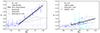 |
Fig. 1. Constrained relations between the UV continuum slope, β, and the absolute UV magnitude at z = 6 (left) and z = 9 (right). Small crosses represent intrinsic values. Points represent dust-attenuated values. The solid black lines fit observations by Bouwens et al. (2014) at z = 6 and by Atek et al. (2023) at z ≥ 9. Grey dashed and dash-dotted lines show models by Vijayan et al. (2021) and Kannan et al. (2022) that fail to reproduce these observations. |
For galaxies with MUV, 0 < −19, we compute the (β, MUV) pair needed to follow these observed relations, starting with the intrinsic values (β0, MUV, 0). First, we compute the average intrinsic slope, ⟨β0⟩= − 2.37, for all galaxies brighter than MUV, 0 = −19. For each galaxy, we compute the deviation from this average, Δβ0 = β0 − ⟨β0⟩. This scatter is kept invariant because it is due to the intrinsic differences in the age of the stellar populations. Then, a first guess of the attenuated value is
 (1)
(1)
where x = MUV, 0, the intrinsic magnitude. The dust attenuation, AUV, is computed using the definition of the UV slope and the relation between intrinsic and attenuated values:
 (2)
(2)
where C = −0.55 assuming a Calzetti attenuation law (Calzetti et al. 2000). Therefore, the attenuated magnitude is MUV = MUV, 0 + AUV. Using this value, we recompute β using Eq. (1) with x = MUV. The new β is now consistent with the dust attenuated magnitude.
Figure 1 shows the β–MUV relations from FirstLight galaxies, constrained by observations. Other attempts to compute dust attenuation using radiative transfer calculations (Vijayan et al. 2021; Kannan et al. 2022) are not able to reproduce relatively red slopes, β > −1.8, which are very common in bright sources, MUV < −20 at z ≃ 6 (Bouwens et al. 2014). Our approach to dust attenuation reproduces these red slopes by construction. Future attempts using radiative transfer calculations will compute dust attenuation self-consistently from galaxy properties. This requires high-resolution simulations that resolve the dust-star mixture accurately (Mushtaq et al. 2023; Esmerian & Gnedin 2024), as well as the holes and clumps in the dust distribution.
At higher redshifts, z ≥ 9, JWST observations indicate lower attenuations at a fixed UV magnitude (Atek et al. 2023; Franco et al. 2023; Heintz et al. 2024). This could be due to a lower dust or metal content in these first galaxies. Our estimation of dust attenuation is constrained by these observations but larger samples of galaxies with accurately values of β at z ≥ 9 are needed to confirm these trends.
4. Results
4.1. Evolution of the UV luminosity function
Using the dust-attenuated rest-frame UV absolute magnitudes constrained by the observed evolution of the β–MUV relation between z = 6 and z ≥ 9, we can generate the UV luminosity functions at different redshifts and compare with pre-JWST and JWST observations (Figure 2). At z = 6, FirstLight galaxies are consistent with the compilation of pre-JWST observations by Bouwens et al. (2021), although the faint end falls slightly below observations by about 0.1 dex.
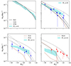 |
Fig. 2. Evolution of the UV luminosity function from z = 6 to z = 13. The cyan regions represent the FirstLight simulations with Poisson uncertainties. JWST observations are marked by blue circles (Harikane et al. 2023), blue squares (Finkelstein et al. 2024), red circles (Bouwens et al. 2022), and red squares (Yan et al. 2023). Pre-JWST observations are shown by black lines (Bouwens et al. 2021). The fiducial models by Ferrara et al. (2023) (grey dash-dotted line), Yung et al. (2023) (brown dashed lines), Mauerhofer & Dayal (2023) (brown dash-dotted lines), and Gelli et al. (2024) (gray dotted lines) fail to reproduce JWST observations at z ≥ 9. FirstLight results lie in between FFB models with ϵmax = 0.2 and 1 (gray solid lines). |
At z = 9, The FirstLight simulations are consistent with new JWST observations (Harikane et al. 2023; Finkelstein et al. 2024). The number densities for bright sources, MUV < −20, are higher than in pre-JWST data. This trend continues at higher redshifts, z = 11 and 13, where FirstLight number densities are remarkably similar to the observed JWST estimates (Bouwens et al. 2022; Yan et al. 2023), although the uncertainties are high for these relatively small samples. In particular, FirstLight lacks statistics for very bright galaxies, MUV < −20 at the highest redshift bin, z = 13. Most probably this is due to the relatively small volume of these simulations. On the other hand, the two galaxies with spectroscopic redshifts at z = 13 − 14 are not exceptionally bright, MUV > −21 (Carniani et al. 2024). More spectroscopic redshifts of high-z candidates are needed for a better constrain of the high-luminosity end of the UVLF at these extremely high redshifts.
FirstLight predictions are higher than recents models that assume a constant galaxy efficiency (e.g. Yung et al. 2023; Mauerhofer & Dayal 2023; Gelli et al. 2024), especially for bright galaxies at z = 13. Other models, such as Ferrara et al. (2023), overproduce fainter galaxies in comparison with FirstLight and JWST results. The closest model is FFB with ϵmax = 0.2 (Dekel et al. 2023; Li et al. 2024).
Bright galaxies form earlier and faster than fainter galaxies at z ≥ 9 and therefore, their number density increases slowly at later times. For example, the number density of galaxies with MUV = −19 increases by two orders of magnitudes from z = 13 to z = 6. During the same period of time, the number density of galaxies with MUV = −20 increases only by a factor of 60. For a better understanding of this galaxy growth, we need to link these UV magnitudes with the virial mass of the halos hosting these galaxies. According to gas-regulator models (Bouché et al. 2010; Lilly et al. 2013; Dekel et al. 2013; Dekel & Mandelker 2014), the halo mass at a given redshift sets the amount of gas accreted into the galaxy and regulates the subsequent star formation at the central galaxy. Then, we can look at the galaxy growth at different halo masses and redshifts.
4.2. Scaling relations: Mvir vs. MUV
The relation between the UV magnitude and the stellar (or halo) mass evolves with redshift (Ceverino et al. 2019). This is due to the evolution of the specific star-formation rate (sSFR), partially driven by the specific halo mass growth, Ṁvir/Mvir ∝ (1 + z)5/2 (Dekel et al. 2013; Dekel & Mandelker 2014; Ceverino et al. 2018). Figure 3 shows the evolution of the relation between the UV magnitude and the virial mass, Mvir (Bryan & Norman 1998). A bright galaxy with MUV = −20 at z ≃ 6, corresponding to an Universe age of tU ≃ 1 Gyr, typically lives in a halo of mass log(Mvir/M⊙) = 10.8 ± 0.1. A second galaxy with the same rest-frame UV magnitude but at z = 12 (tU ≃ 0.4 Gyr) has a halo of mass log(Mvir/M⊙)≃10.4, a factor three lower than in the first case. Galaxies with masses similar to the second halo are therefore more abundant than galaxies with the first halo mass at z = 12. As a result, the bright sources have higher number densities at z = 12 than in the case of no evolution in the MUV − Mvir relation.
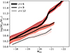 |
Fig. 3. Virial mass versus MUV at z ≃ 6, 9 and 12 in FirstLight galaxies. The colored regions cover the 25 and 75% quantiles. As redshift increases, the UV luminosity increases at a fixed virial mass. |
For brighter objects, MUV < −20, there is a change in the slope of the relation due to dust attenuation at z = 6. This increases the difference described above between galaxies with MUV < −20 at different redshifts. Unfortunately, there are no objects with MUV < −21 at higher redshifts within the simulated volume and we cannot compare their virial masses at the brightest end. Therefore, most of the evolution seen in Figure 3 is insensitive to the dust attenuation model.
For a fixed virial mass, a halo with log(Mvir/M⊙) = 10.6 at z ≃ 6 typically hosts a relatively low luminosity galaxy with MUV ≃ −19. Another halo of the same mass at z ≃ 12 contains a galaxy two magnitudes brighter, MUV ≃ −21. This evolution at a given halo mass can also be due to a higher conversion of accreted gas into stars for a given halo growth at higher redshifts. We will explore this possibility in the next section.
4.3. Instantaneous galaxy formation efficiency
The instantaneous galaxy formation efficiency can be defined as the ratio between the stellar and halo mass growth,
 (3)
(3)
normalized to the universal baryonic fraction, fB. This ratio removes the explicit redshift dependence, (1 + z)5/2, described above. It mainly depends on the ability of accreted baryons to contribute to the galaxy stellar mass growth: the penetration of gas streams into the halo center and the regulation of the gas-stars cycle by feedback. These processes depend on halo mass. For example, feedback regulates strongly the formation of stars in low-mass halos with shallow potential wells (Dekel & Silk 1986). At a fixed halo mass, this efficiency may increase with redshift due to an increase in the penetration factor or due to a decrease in the mass-loading factor of galactic outflows (Dekel & Mandelker 2014). In the FFB scenario, this is due to an increase in the gas density (Dekel et al. 2023). The galaxy efficiency can vary with redshift due to alterations in these processes.
We compute the instantaneous efficiency using all snapshots stored every 10 Myr. Mass variations, ΔM* and ΔMvir between consecutive snapshots of the same galaxy can be compared within a given redshift bin. Figure 4 shows the evolution of this efficiency from z ≃ 6 to 12. There is a significant increase of this efficiency with redshift. At a fixed halo mass, Mvir ≃ 1011 M⊙, the efficiency increases a factor 3 between 10% at z ≃ 6 and ∼30% at z ≃ 12. They are similar to the values required for reconciling UV and halo mass functions at z ≥ 10 (Inayoshi et al. 2022). For more massive galaxies, Mvir ≃ 1011.5 M⊙, the values can be higher, although there is a flattening of the efficiency, with maximum values of ∼40% at z ≃ 6 on average. These massive galaxies are absent within the limited volume of these simulations at redshift higher than 7 and we cannot constrain the evolution at this massive end.
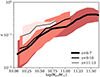 |
Fig. 4. Instantaneous galaxy formation efficiency, ϵ = Ṁ∗/(ṀvirfB), at different redshifts. The colored regions cover the 25 and 75% quantiles. The efficiency increases with mass and redshift. |
4.4. Integrated galaxy formation efficiency
The integrated galaxy formation efficiency differs from the instantaneous efficiency because it involves time-integrated values:
 (4)
(4)
where M* is the stellar mass of the galaxy. Figure 5 shows the evolution of this efficiency with redshift. It has a similar dependence with virial mass than the instantaneous efficiency although its redshift evolution is milder. At a fixed virial mass, Mvir ≃ 1011 M⊙, the integrated efficiency doubles its value from ϵ* ≃ 0.1 at z ≃ 6 to ϵ* ≃ 0.2 at z ≃ 10. At higher redshifts, z ≃ 12, the apparent lack of evolution at this massive end is due to a small number of galaxies in this bin. At lower masses, the evolution is below a factor 2 and the efficiency remains at lower values, ϵ* < 0.1, because feedback regulates efficiently the SF process at low masses. At a given redshift, the integrated efficiency is slightly lower than the instantaneous efficiency, Eq. (3), by a factor of about 2. This is because the integrated efficiency is based on the time-integral of previous values of Ṁ∗/Ṁvir, which are generally lower than the current value because of the galaxy growth and the mass-dependence described in Figure 4.
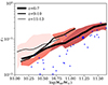 |
Fig. 5. Integrated galaxy formation efficiency, ϵ* = M*/(MvirfB), at different redshifts. The lines are the same as in Fig. fig:epsilon. Blue points represent the VELA-6 simulations (Ceverino et al. 2023) at z = 4 and the blue star represents a z = 0 galaxy from Ceverino et al. (2017b). As redshift increases, the efficiency increases at a fixed virial mass. |
This redshift dependency continues toward lower redshifts. Other simulations with the same feedback model show lower efficiencies at z < 5. This is especially relevant at low masses, Mvir < 1011M⊙, where feedback is most efficient. For example, the VELA-6 simulations (Ceverino et al. 2023) have a factor 3–4 lower efficiency at z = 4 than FirstLight galaxies with the same virial mass, Mvir ≃ 1010.5M⊙, at z = 12. On the other hand, the AGORA galaxy at z ≃ 0 (Ceverino et al. 2017b) has a more massive halo, Mvir ≃ 1011.2M⊙ and it reaches the same efficiency, ϵ* ≃ 0.1, than FirstLight galaxies of similar mass at z ≃ 6. There are no counterparts at higher redshift and therefore we cannot see if the efficiency is higher at the high-mass end but the extrapolation from lower masses hints to that possibility. We conclude that the integrated efficiency evolves with time, but this evolution depends on halo mass. Ultimately, it is related to the competition between the penetration of gas flows into galaxies and the outflows driven by feedback.
4.5. Galaxy stellar mass function
The evolution in the integrated galaxy formation efficiency drives a non-homogeneous evolution of the galaxy stellar mass function (Figure 6). This is consistent with recent JWST results at z ≃ 9 (Harvey et al. 2024; Weibel et al. 2024) within observational uncertainties. Low-mass galaxies, M* = 108.5 M⊙, grow in numbers by a factor 5 between z = 11 and z = 9. Slightly more massive galaxies, M* = 109 M⊙, grow by a factor 10 within the same period. As a result, they are more abundant than in other models (Lovell et al. 2021; Yung et al. 2023; Mauerhofer & Dayal 2023) with lower efficiencies at z ≥ 10. FFB models with ϵmax = 0.2 show consistent results at z = 6 but higher number densities than FirstLight at z ≥ 9.
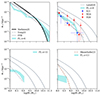 |
Fig. 6. Evolution of the galaxy stellar mass function from z = 6 to z = 13. FirstLight is consistent with pre-JWST observations (Stefanon et al. 2021) at z = 6 but it shows higher numbers of massive galaxies at z = 9, in agreement with JWST results (Harvey et al. 2024; Weibel et al. 2024). Gray solid lines represents FFB model with ϵmax = 0.2 and 1. Simulations by Lovell et al. (2021) and semi-analytical models by Yung et al. (2023) and Mauerhofer & Dayal (2023) show lower values at high masses. |
Galaxies more massive than 109 M⊙ at z > 11 are absent within these cosmological volumes. Larger volumes are needed to simulate these massive and relatively rare halos. FirstLight also predicts higher number densities than pre-JWST observations (Stefanon et al. 2021) at z ≃ 9, even after different assumptions on IMF and cosmology are corrected. However, this excess almost disappears at z ≃ 6, as the integrated efficiency decreases with time.
The lower numbers found at low masses indicate some incompleteness in the small and intermediate boxes at the lowest redshifts, z ≃ 6 (Ceverino et al. 2018). However, the agreement between observations and FirstLight at high masses, M* > 1010 M⊙, is good within uncertainties. There are ways to correct for incompleteness (Ma et al. 2018; Lovell et al. 2021) but they are not used here, as we are focusing on high masses and redshifts, where FirstLight includes all halos available within the simulated volumes.
5. Discussion
5.1. Comparison of integrated efficiency from observations and other models
The integrated efficiency, Eq. (4), has been computed in different works but there is no consensus on whether it is time dependent or independent. Figure 7 shows a comparison between FirstLight results and other works at two different redshifts. Stefanon et al. (2021) use the deepest Spitzer and HST observations and show that the integrated efficiency increases with mass but there is no significant evolution from z ≃ 10 to z ≃ 6. FirstLight is consistent with their results at z = 6 but it is significantly higher at z ≃ 9 by a factor 2–4. Their low values are mostly driven by the accelerated evolution of the galaxy stellar mass function between z ≃ 9 and z ≃ 6 (Figure 6), inconsistent with the FirstLight results. The semi-empirical model by Tacchella et al. (2018) combine UVLF from HST observations at z = 5 − 10 and dark-matter halo accretion rates from N-body simulations. They also conclude that the integrated efficiency is redshift-independent in that redshift range. Therefore, they agree with FirstLight at z = 6 but they are significantly lower at z = 9, in agreement with the previous observations. A similar approach is used in others abundance-matching models (e.g. Behroozi et al. 2019) that use pre-JWST observations to infer relatively low efficiencies at high redshifts.
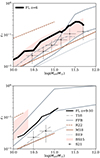 |
Fig. 7. Comparison of the integrated efficiency at z = 6 (top) and z ≃ 9 (bottom) between FirstLight (solid black lines, as in Figure 5), pre-JWST observations by Stefanon et al. (2021) (points with error bars), SPHINX (dashed) and FIRE-2 (solid) simulations, and semi-empirical models by Behroozi & Silk (2015) (red contour), Tacchella et al. (2018) (dot-dashed), Behroozi et al. (2019) (dotted), and Li et al. (2024) models of FFB with ϵmax = 0.2 and 1 (solid grey lines). |
Other cosmological simulations, like SPHINX (Rosdahl et al. 2018; Katz et al. 2023), have a high efficiency. It therefore over-predicts the values at low redshifts, z = 6, where observational estimates are more robust. On the other hand, the FIRE-2 simulations (Ma et al. 2018) under-predict the efficiency at the same redshift. Both simulations have roughly constant values with time because feedback is either too strong (FIRE) or too weak (SPHINX) to self-regulate the combined cycle of SF and feedback.
Other models consider a redshift-dependent efficiency, which is qualitatively consistent with FirstLight. For example, Behroozi & Silk (2015) use a variable ratio between the sSFR and the halo specific mass accretion rate to predict the galaxy efficiency to z ≃ 15. Although their estimates are higher than in previous redshift-independent models, they are consistent with FirstLight at z = 6. At z ≃ 10, their uncertainties are higher and these predictions are also above FirstLight by a factor of a few.
In the FFB scenario (Dekel et al. 2023), the efficiency is a function of mass and redshift, assuming a maximum value, ϵmax, above a mass threshold, Mvir, fbb, that declines with redshift (Li et al. 2024). For halo masses below that threshold, feedback regulates the SF cycle and maintains a relatively low SF efficiency. Their minimum model with ϵmax = 0.2 is consistent with FirstLight at z = 10. Order-unity efficiencies, ϵmax ≃ 1, are excluded within the mass range explored by FirstLight. At z = 6, the maximum efficiency in FirstLight is close to ϵ* ≃ 0.3. This is consistent with the cumulative values estimated using MIRI photometry of massive galaxies (Wang et al. 2024). This maximum happens at Mvir ≃ 1011.5 M⊙, slightly below the FFB threshold, Mvir, fbb ≃ 1011.75 M⊙ at z = 6. As a result, the FirstLight efficiencies at z = 6 are higher than in the FFB scenario at lower masses, Mvir < 1011 M⊙, a mass range in which the efficiencies in Li et al. (2024) get closer to the Behroozi et al. (2019) model, which shows low values.
5.2. Evolution of the cosmic UV and stellar mass density
The integration of the UVLF (Figure 2) to MUV < −17 at different redshifts gives an estimate of the comoving cosmic UV density (Figure 8), which can we compared with other works. Due to the increase of the efficiency at z ≥ 9, the values are above the models with redshift-independent efficiency (Tacchella et al. 2018; Harikane et al. 2022). There is no sign of accelerated evolution between z = 10 and z = 8, as seen in pre-JWST observations (Oesch et al. 2018). In fact, a gentle evolution, approximately fitted by log(ρUV)∝ − 0.7(1 + z), is consistent with most JWST observations up to z ≃ 13. FirstLight results are only slightly below observations by 0.2–0.3 dex at z ≥ 11, still in between the estimated uncertainties. Larger samples of galaxies with robust redshift estimations are necessary for more accurate constrains.
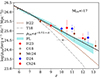 |
Fig. 8. Evolution of the cosmic UV density for galaxies with MUV < −17. FirstLight values are above the models with redshift-independent efficiency by Harikane et al. (2022) and Tacchella et al. (2018), as well as other pre-JWST observations at z ≥ 10 (Oesch et al. 2018). JWST values (Harikane et al. 2023; McLeod et al. 2024; Chemerynska et al. 2024; Donnan et al. 2024) are consistent with FirstLight within the estimated uncertainties. |
The comoving cosmic stellar mass density, for all galaxies more massive than 108 M⊙, provides another overall comparison with previous works (Figure 9). At z ≃ 6, FirstLight values are slightly lower than other models. This is due to the slight incompleteness at low masses discussed above. At higher redshifts, z > 9, models that assume a constant efficiency (Tacchella et al. 2018) and pre-JWST observations (Stefanon et al. 2021) show a much more drastic drop due to the lack of massive galaxies. However, FirstLight values show a smooth evolution, log(ρ*)∝ − (1 + z), due to the high efficiency at these high redshifts. Future JWST observations are needed to confirm the gentle rise of the stellar mass density at these early times.
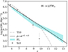 |
Fig. 9. Evolution of the cosmic stellar mass density for galaxies with M* > 108M⊙. FirstLight-derived densities are higher than pre-JWST values at z > 9 (Stefanon et al. 2021) and previous models with a redshift-independent efficiency (Tacchella et al. 2018). |
5.3. Drivers of galaxy efficiency
Different galaxy conditions determine different efficiencies in the galaxy growth with respect to halo growth, Eq. (3). For example, the baryonic inflow from the halo to the galaxy depends on the cycle from the circumgalactic medium to the star-forming interstellar medium. Variations in this cycle could modify the rate of galaxy growth even at a fixed halo mass growth (Dekel et al. 2013). Feedback regulates the SF process by driving galactic outflows or by decreasing the fraction of cold and dense, star-forming gas (Ceverino et al. 2014). However, feedback depends on gas conditions, particularly on its density (Dekel & Silk 1986; Dekel et al. 2023). Therefore, galaxy efficiency can vary with redshift as gas within galaxies evolves with time. A more in-depth study to identify the main driver of this evolution is beyond the scope of this paper, but we can provide some hints.
In Figure 10 we compare two examples of galaxies with a similar halo mass, Mvir ≃ 1011 M⊙, but different galaxy efficiencies at different redshifts. The first galaxy at z = 9 has a high efficiency, ϵ ≃ 0.3 and ϵ* ≃ 0.6. A significant fraction of the galaxy, especially the center and off-center clumps, has very high densities, n ≥ 3000 cm−3. The corresponding free-fall time is lower than 1 Myr and the effect of feedback drastically decreases at these high densities, according to the FFB scenario (Dekel et al. 2023). Therefore, the SFR surface density reaches extreme values, ΣSFR ≥ 103 M⊙ yr−1 kpc−2, similar to the observational estimates in a very dense star-forming environment of a z = 12 galaxy (Calabro et al. 2024).
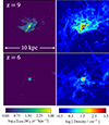 |
Fig. 10. Example of a highly efficient galaxy at z = 9 (top) and a galaxy at z = 6 with the same halo mass of Mvir ≃ 1011 M⊙ but lower efficiency (bottom). Left panels show the star formation rate surface density and right panels depict the gas density, averaged along the line of sight. |
The second example at z = 6 has a lower efficiency, ϵ ≃ 0.1 and ϵ* ≃ 0.09. Both the gas density and the SFR surface density are much lower than in the previous example, although consistent with observations that spatially resolve the Kennicutt–Schmidt relation at z = 7 (Vallini et al. 2024). This galaxy has the same amount of gas within the virial radius as in the previous case (Mgas, halo = 2 × 10¹⁰ M⊙), but only 7% of this mass is forming stars. This fraction increases to 30% in the first galaxy at z = 9. As a result, the star-formation rate of this highly efficient galaxy is ten times higher than the other example at lower redshift. This also translates into a factor-of-two shorter gas depletion time, tD = Mgas, galaxy/SFR = 60 Myr. This value is close to the average at z = 10 (Ceverino et al. 2018), but it is a factor 30 shorter than in local galaxies (Leroy et al. 2008; Saintonge & Catinella 2022; Sun et al. 2023b).We conclude that the gas densities in SF bursts at extremely high redshifts, z ≥ 9, facilitates very high galaxy efficiencies, ϵmax ≃ 0.3 − 0.4, at moderate halo masses, Mvir ≃ 1011 M⊙. Future simulations of bigger volumes will explore higher masses and possible higher efficiencies in more extreme and rare halos at high redshifts.
6. Conclusions
We use the FirstLight database of 377 zoom-in cosmological simulations of a mass-complete sample of galaxies with a spatial resolution of 10–20 parsecs in a (60 Mpc)3 comoving volume, to understand galaxy growth at extremely high redshifts, z = 9 − 13.
The main highlights of this paper are the following:
-
FirstLight contains a high number of bright galaxies, MUV ≃ −20, consistent with JWST data.
-
The relation between MUV and halo mass evolves with redshift. It is mostly independent of the dust attenuation model and it is due to higher mass accretion and SF efficiency at higher redshifts.
-
The galaxy formation efficiency, Eqs. (3) and (4), increases significantly with mass and redshift. At a fixed mass, galactic halos at extremely high redshifts convert gas into stars at a higher rate than at lower redshifts.
-
The number density of massive galaxies, M* ≃ 109 M⊙ at z ≥ 9, are higher than in other models with a constant star-formation efficiency.
-
The high gas densities in these SF bursts at z ≥ 9 enable these high efficiencies (Figure 10), in qualitative agreement with the scenario of Feedback Free Starbursts (FFB) at high redshifts.
In spite of this success in reproducing current JWST observations, FirstLight simulations also have some caveats. For example, they do not include the radiative transfer of ionizing photons, instead assuming that these photons are mostly absorbed in the immediate vicinity of the massive stars producing them. Therefore, radiative feedback only affects gas close to massive stars; the effects of the leakage of this radiation into the interstellar medium is not included. This could modify the gas conditions further away from the star-forming regions (Emerick et al. 2019). Future simulations should include these radiative-transfer effects.
The maximum resolution achieved in FirstLight (10–20 pc) also imposes some limitations. This is not enough to properly resolve the star forming clouds that are predicted to have comparable sizes of ∼10 pc. The feedback-free starbursts with order-unity SF efficiency are predicted to occur in these clouds because of their high gas densities. High-resolution simulations of the formation of individual massive clusters find these high SF efficiencies in high-density clouds. (e.g. Kim et al. 2016; Fukushima & Yajima 2021; Calura et al. 2022; Polak et al. 2024). In the FirstLight simulations, similar high densities happen on larger scales at higher redshifts (Figure 10) because of the compact nature of these galaxies. Therefore, the efficiency increases with redshift but its maximum value, ϵmax ≃ 0.2 − 0.3, is far away from the order-unity efficiency expected within feedback-free starbursts. Still, this galaxy-averaged efficiency is consistent with the fiducial FFB model that best agree with JWST observations (Li et al. 2024).
Other cosmological simulations (Rosdahl et al. 2018; Ma et al. 2018) do not show this evolution of the efficiency because their feedback is either too weak or too strong to self-regulate the combined cycle of SF and feedback at high-z. The model included in FirstLight has the combined effect of thermal, kinetic and radiative feedback. At high densities, both thermal and kinetic modes are quickly dissipated by shocks and radiative cooling. This reduces the effect of feedback in high densities conditions at high redshifts.
We conclude that FirstLight simulations can reproduce different conditions of galaxy formation across cosmic history. Relatively massive galaxies at extremely high redshifts have a low efficiency of feedback and therefore star formation and galaxy growth can proceed faster than at later times. Other modern cosmological simulations with phenomenological feedback models (Pillepich et al. 2018; Davé et al. 2019) include a decrease of the mass in galactic outflows with increasing galaxy mass. However, these models are calibrated on observations at lower redshifts and they may fail at much early times, when gas densities are much higher. Future observations by JWST will utilize multi-line diagnostics to infer the gas density in star-forming regions at these high-z and they can validate the redshift evolution advocated here.
The next generation of cosmological simulations must reproduce the galaxy conditions across different redshifts, from the local Universe at z = 0 well into the dark epoch, z = 10 − 20, before the reionization of the Universe. Parsec scale resolution is probably required in order to properly resolve star formation and self-regulation of stellar birth at this epoch, including key processes such as the turbulence in the dense interstellar medium, feedback from black holes and AGN, as well as magnetic fields and cosmic rays.
Acknowledgments
We thank the referee, Avishai Dekel, for constructive suggestions that improve the quality of this paper. We acknowledge stimulating discussions with Joel Primack and Anatoly Klypin. We thank Viola Gelli and Zhaozhou Li for sharing their data. The authors gratefully acknowledge the Gauss Center for Supercomputing for funding this project by providing computing time on the GCS Supercomputer SuperMUC at Leibniz Supercomputing Center (Project ID: pr92za). The authors thankfully acknowledge the computer resources at MareNostrum and the technical support provided by the Barcelona Supercomputing Center (RES-AECT-2020-3-0019). This work used the v2.1 of the Binary Population and Spectral Synthesis (BPASS) models as last described in Eldridge et al. (2017). DC is a Ramon-Cajal Researcher and is supported by the Ministerio de Ciencia, Innovación y Universidades (MICIU/FEDER) under research grant PID2021-122603NB-C21. YN acknowledges funding from JSPS KAKENHI Grant Number 23KJ0728 and a JSR fellowship. RSK and SCOG acknowledge funding from the ERC via Synergy Grant “ECOGAL” (project ID 855130), from the German Excellence Strategy via the Heidelberg Cluster of Excellence (EXC 2181 – 390900948) “STRUCTURES”, and from the German Ministry for Economic Affairs and Climate Action in project “MAINN” (funding ID 50OO2206). RSK and SCOG also thank for computing resources provided by the Ministry of Science, Research and the Arts (MWK) of the State of Baden-Württemberg through bwHPC and DFG through grant INST 35/1134-1 FUGG and for data storage at SDS@hd through grant INST 35/1314-1 FUGG.
References
- Abel, T., Bryan, G. L., & Norman, M. L. 2002, Science, 295, 93 [CrossRef] [Google Scholar]
- Adams, N. J., Conselice, C. J., Ferreira, L., et al. 2023, MNRAS, 518, 4755 [Google Scholar]
- Atek, H., Chemerynska, I., Wang, B., et al. 2023, MNRAS, 524, 5486 [NASA ADS] [CrossRef] [Google Scholar]
- Behroozi, P., Wechsler, R. H., Hearin, A. P., & Conroy, C. 2019, MNRAS, 488, 3143 [NASA ADS] [CrossRef] [Google Scholar]
- Behroozi, P. S., & Silk, J. 2015, ApJ, 799, 32 [NASA ADS] [CrossRef] [Google Scholar]
- Bouché, N., Dekel, A., Genzel, R., et al. 2010, ApJ, 718, 1001 [Google Scholar]
- Bouwens, R. J., Illingworth, G. D., Oesch, P. A., et al. 2014, ApJ, 793, 115 [Google Scholar]
- Bouwens, R. J., Oesch, P. A., Stefanon, M., et al. 2021, AJ, 162, 47 [NASA ADS] [CrossRef] [Google Scholar]
- Bouwens, R. J., Illingworth, G., Ellis, R. S., Oesch, P., & Stefanon, M. 2022, ApJ, 940, 55 [NASA ADS] [CrossRef] [Google Scholar]
- Bromm, V., Coppi, P. S., & Larson, R. B. 2002, ApJ, 564, 23 [Google Scholar]
- Bryan, G. L., & Norman, M. L. 1998, ApJ, 495, 80 [NASA ADS] [CrossRef] [Google Scholar]
- Calabro, A., Castellano, M., Zavala, J. A., et al. 2024, ApJ, submitted [arXiv:2403.12683] [Google Scholar]
- Calura, F., Lupi, A., Rosdahl, J., et al. 2022, MNRAS, 516, 5914 [Google Scholar]
- Calzetti, D., Armus, L., Bohlin, R. C., et al. 2000, ApJ, 533, 682 [NASA ADS] [CrossRef] [Google Scholar]
- Carniani, S., Hainline, K., D’Eugenio, F., et al. 2024, ArXiv e-prints [arXiv:2405.18485] [Google Scholar]
- Casey, C. M., Akins, H. B., Shuntov, M., et al. 2024, ApJ, 965, 98 [NASA ADS] [CrossRef] [Google Scholar]
- Castellano, M., Fontana, A., Treu, T., et al. 2022, ApJ, 938, L15 [NASA ADS] [CrossRef] [Google Scholar]
- Ceverino, D., & Klypin, A. 2009, ApJ, 695, 292 [Google Scholar]
- Ceverino, D., Dekel, A., & Bournaud, F. 2010, MNRAS, 404, 2151 [NASA ADS] [Google Scholar]
- Ceverino, D., Klypin, A., Klimek, E. S., et al. 2014, MNRAS, 442, 1545 [NASA ADS] [CrossRef] [Google Scholar]
- Ceverino, D., Glover, S. C. O., & Klessen, R. S. 2017a, MNRAS, 470, 2791 [NASA ADS] [CrossRef] [Google Scholar]
- Ceverino, D., Primack, J., Dekel, A., & Kassin, S. A. 2017b, MNRAS, 467, 2664 [NASA ADS] [CrossRef] [Google Scholar]
- Ceverino, D., Klessen, R. S., & Glover, S. C. O. 2018, MNRAS, 480, 4842 [NASA ADS] [Google Scholar]
- Ceverino, D., Klessen, R. S., & Glover, S. C. O. 2019, MNRAS, 484, 1366 [NASA ADS] [CrossRef] [Google Scholar]
- Ceverino, D., Hirschmann, M., Klessen, R. S., et al. 2021, MNRAS, 504, 4472 [NASA ADS] [CrossRef] [Google Scholar]
- Ceverino, D., Mandelker, N., Snyder, G. F., et al. 2023, MNRAS, 522, 3912 [NASA ADS] [CrossRef] [Google Scholar]
- Chemerynska, I., Atek, H., Furtak, L. J., et al. 2024, MNRAS, 531, 2615 [NASA ADS] [CrossRef] [Google Scholar]
- Curti, M., D’Eugenio, F., Carniani, S., et al. 2023, MNRAS, 518, 425 [Google Scholar]
- Davé, R., Anglés-Alcázar, D., Narayanan, D., et al. 2019, MNRAS, 486, 2827 [Google Scholar]
- Dekel, A., & Mandelker, N. 2014, MNRAS, 444, 2071 [NASA ADS] [CrossRef] [Google Scholar]
- Dekel, A., & Silk, J. 1986, ApJ, 303, 39 [Google Scholar]
- Dekel, A., Birnboim, Y., Engel, G., et al. 2009, Nature, 457, 451 [Google Scholar]
- Dekel, A., Zolotov, A., Tweed, D., et al. 2013, MNRAS, 435, 999 [Google Scholar]
- Dekel, A., Sarkar, K. C., Birnboim, Y., Mandelker, N., & Li, Z. 2023, MNRAS, 523, 3201 [NASA ADS] [CrossRef] [Google Scholar]
- Donnan, C. T., McLeod, D. J., Dunlop, J. S., et al. 2023, MNRAS, 518, 6011 [Google Scholar]
- Donnan, C. T., McLure, R. J., Dunlop, J. S., et al. 2024, MNRAS, submitted [arXiv:2403.03171] [Google Scholar]
- Eldridge, J. J., Stanway, E. R., Xiao, L., et al. 2017, PASA, 34, e058 [Google Scholar]
- Emerick, A., Bryan, G. L., & Mac Low, M.-M. 2019, MNRAS, 482, 1304 [NASA ADS] [CrossRef] [Google Scholar]
- Esmerian, C. J., & Gnedin, N. Y. 2024, ApJ, 968, 113 [NASA ADS] [CrossRef] [Google Scholar]
- Ferrara, A., Pallottini, A., & Dayal, P. 2023, MNRAS, 522, 3986 [NASA ADS] [CrossRef] [Google Scholar]
- Fichtner, Y. A., Mackey, J., Grassitelli, L., Romano-Díaz, E., & Porciani, C. 2024, A&A, in press, https://doi.org/10.1051/0004-6361/202449638 [Google Scholar]
- Finkelstein, S. L., Leung, G. C. K., Bagley, M. B., et al. 2024, ApJ, 969, L2 [NASA ADS] [CrossRef] [Google Scholar]
- Franco, M., Akins, H. B., Casey, C. M., et al. 2023, ApJ, submitted [arXiv:2308.00751] [Google Scholar]
- Fukushima, H., & Yajima, H. 2021, MNRAS, 506, 5512 [NASA ADS] [CrossRef] [Google Scholar]
- Gelli, V., Mason, C., & Hayward, C. C. 2024, ApJ, submitted [arXiv:2405.13108] [Google Scholar]
- Hainline, K. N., Johnson, B. D., Robertson, B., et al. 2024, ApJ, 964, 71 [CrossRef] [Google Scholar]
- Harikane, Y., Ono, Y., Ouchi, M., et al. 2022, ApJS, 259, 20 [NASA ADS] [CrossRef] [Google Scholar]
- Harikane, Y., Ouchi, M., Oguri, M., et al. 2023, ApJS, 265, 5 [NASA ADS] [CrossRef] [Google Scholar]
- Harvey, T., Conselice, C., Adams, N. J., et al. 2024, ApJ, submitted [arXiv:{2403.03908}] [Google Scholar]
- Heintz, K. E., Brammer, G. B., Watson, D., et al. 2024, A&A, submitted [arXiv:2404.02211] [Google Scholar]
- Inayoshi, K., Harikane, Y., Inoue, A. K., Li, W., & Ho, L. C. 2022, ApJ, 938, L10 [NASA ADS] [CrossRef] [Google Scholar]
- Kannan, R., Smith, A., Garaldi, E., et al. 2022, MNRAS, 514, 3857 [CrossRef] [Google Scholar]
- Katz, H., Galligan, T. P., Kimm, T., et al. 2019, MNRAS, 487, 5902 [NASA ADS] [CrossRef] [Google Scholar]
- Katz, H., Rosdahl, J., Kimm, T., et al. 2023, Open J. Astrophys., 6, 44 [NASA ADS] [CrossRef] [Google Scholar]
- Kennicutt, R. C., Jr 1998, ApJ, 498, 541 [Google Scholar]
- Kim, J.-G., Kim, W.-T., & Ostriker, E. C. 2016, ApJ, 819, 137 [NASA ADS] [Google Scholar]
- Klessen, R. S., & Glover, S. C. O. 2023, ARA&A, 61, 65 [NASA ADS] [CrossRef] [Google Scholar]
- Kravtsov, A. V. 2003, ApJ, 590, L1 [NASA ADS] [CrossRef] [Google Scholar]
- Kravtsov, A. V., Klypin, A. A., & Khokhlov, A. M. 1997, ApJS, 111, 73 [Google Scholar]
- Langan, I., Ceverino, D., & Finlator, K. 2020, MNRAS, 494, 1988 [NASA ADS] [CrossRef] [Google Scholar]
- Leroy, A. K., Walter, F., Brinks, E., et al. 2008, AJ, 136, 2782 [Google Scholar]
- Leśniewska, A., & Michałowski, M. J. 2019, A&A, 624, L13 [Google Scholar]
- Leung, G. C. K., Bagley, M. B., Finkelstein, S. L., et al. 2023, ApJ, 954, L46 [NASA ADS] [CrossRef] [Google Scholar]
- Li, Z., Dekel, A., Sarkar, K. C., et al. 2024, A&A, in press, https://doi.org/10.1051/0004-6361/202348727 [Google Scholar]
- Lilly, S. J., Carollo, C. M., Pipino, A., Renzini, A., & Peng, Y. 2013, ApJ, 772, 119 [NASA ADS] [CrossRef] [Google Scholar]
- Lovell, C. C., Vijayan, A. P., Thomas, P. A., et al. 2021, MNRAS, 500, 2127 [Google Scholar]
- Lovell, C. C., Harrison, I., Harikane, Y., Tacchella, S., & Wilkins, S. M. 2023, MNRAS, 518, 2511 [Google Scholar]
- Ma, X., Hopkins, P. F., Garrison-Kimmel, S., et al. 2018, MNRAS, 478, 1694 [NASA ADS] [CrossRef] [Google Scholar]
- Mason, C. A., Trenti, M., & Treu, T. 2023, MNRAS, 521, 497 [NASA ADS] [CrossRef] [Google Scholar]
- Mauerhofer, V., & Dayal, P. 2023, MNRAS, 526, 2196 [NASA ADS] [CrossRef] [Google Scholar]
- McLeod, D. J., Donnan, C. T., McLure, R. J., et al. 2024, MNRAS, 527, 5004 [Google Scholar]
- Mushtaq, M., Ceverino, D., Klessen, R. S., Reissl, S., & Puttasiddappa, P. H. 2023, MNRAS, 525, 4976 [NASA ADS] [CrossRef] [Google Scholar]
- Naidu, R. P., Oesch, P. A., van Dokkum, P., et al. 2022, ApJ, 940, L14 [NASA ADS] [CrossRef] [Google Scholar]
- Nakazato, Y., Yoshida, N., & Ceverino, D. 2023, ApJ, 953, 140 [NASA ADS] [CrossRef] [Google Scholar]
- Oesch, P. A., Bouwens, R. J., Illingworth, G. D., Labbé, I., & Stefanon, M. 2018, ApJ, 855, 105 [Google Scholar]
- O’Shea, B. W., Wise, J. H., Xu, H., & Norman, M. L. 2015, ApJ, 807, L12 [CrossRef] [Google Scholar]
- Ostriker, E. C., & Shetty, R. 2011, ApJ, 731, 41 [Google Scholar]
- Pallottini, A., Ferrara, A., Decataldo, D., et al. 2019, MNRAS, 487, 1689 [Google Scholar]
- Pérez-González, P. G., Costantin, L., Langeroodi, D., et al. 2023, ApJ, 951, L1 [CrossRef] [Google Scholar]
- Pillepich, A., Springel, V., Nelson, D., et al. 2018, MNRAS, 473, 4077 [Google Scholar]
- Polak, B., Mac Low, M.-M., Klessen, R. S., et al. 2024, A&A, in press, https://doi.org/10.1051/0004-6361/202348840 [Google Scholar]
- Roberts-Borsani, G., Treu, T., Shapley, A., et al. 2024, ApJ, submitted [arXiv:2403.07103] [Google Scholar]
- Rosdahl, J., Katz, H., Blaizot, J., et al. 2018, MNRAS, 479, 994 [NASA ADS] [Google Scholar]
- Saintonge, A., & Catinella, B. 2022, ARA&A, 60, 319 [NASA ADS] [CrossRef] [Google Scholar]
- Schmidt, M. 1959, ApJ, 129, 243 [NASA ADS] [CrossRef] [Google Scholar]
- Shen, X., Vogelsberger, M., Boylan-Kolchin, M., Tacchella, S., & Kannan, R. 2023, MNRAS, 525, 3254 [NASA ADS] [CrossRef] [Google Scholar]
- Stefanon, M., Bouwens, R. J., Labbé, I., et al. 2021, ApJ, 922, 29 [NASA ADS] [CrossRef] [Google Scholar]
- Sun, G., Faucher-Giguère, C.-A., Hayward, C. C., et al. 2023a, ApJ, 955, L35 [CrossRef] [Google Scholar]
- Sun, J., Leroy, A. K., Ostriker, E. C., et al. 2023b, ApJ, 945, L19 [NASA ADS] [CrossRef] [Google Scholar]
- Tacchella, S., Bose, S., Conroy, C., Eisenstein, D. J., & Johnson, B. D. 2018, ApJ, 868, 92 [NASA ADS] [CrossRef] [Google Scholar]
- Tsuna, D., Nakazato, Y., & Hartwig, T. 2023, MNRAS, 526, 4801 [NASA ADS] [CrossRef] [Google Scholar]
- Vallini, L., Witstok, J., Sommovigo, L., et al. 2024, MNRAS, 527, 10 [Google Scholar]
- Venturi, G., Carniani, S., Parlanti, E., et al. 2024, A&A, in press, https://doi.org/10.1051/0004-6361/202449855 [Google Scholar]
- Vijayan, A. P., Lovell, C. C., Wilkins, S. M., et al. 2021, MNRAS, 501, 3289 [NASA ADS] [Google Scholar]
- Wang, T., Sun, H., Zhou, L., et al. 2024, ArXiv e-prints [arXiv:2403.02399] [Google Scholar]
- Weibel, A., Oesch, P. A., Barrufet, L., et al. 2024, MNRAS, submitted, [arXiv:2403.08872] [Google Scholar]
- Xiao, L., Stanway, E. R., & Eldridge, J. J. 2018, MNRAS, 477, 904 [Google Scholar]
- Yan, H., Sun, B., Ma, Z., & Ling, C. 2023, ApJ, submitted, [arXiv:2311.15121] [Google Scholar]
- Yoshida, N., Omukai, K., & Hernquist, L. 2008, Science, 321, 669 [NASA ADS] [CrossRef] [Google Scholar]
- Yung, L. Y. A., Somerville, R. S., Finkelstein, S. L., et al. 2023, MNRAS, 519, 1578 [Google Scholar]
- Yung, L. Y. A., Somerville, R. S., Finkelstein, S. L., Wilkins, S. M., & Gardner, J. P. 2024, MNRAS, 527, 5929 [Google Scholar]
All Figures
|
Fig. 1. Constrained relations between the UV continuum slope, β, and the absolute UV magnitude at z = 6 (left) and z = 9 (right). Small crosses represent intrinsic values. Points represent dust-attenuated values. The solid black lines fit observations by Bouwens et al. (2014) at z = 6 and by Atek et al. (2023) at z ≥ 9. Grey dashed and dash-dotted lines show models by Vijayan et al. (2021) and Kannan et al. (2022) that fail to reproduce these observations. |
| In the text | |
|
Fig. 2. Evolution of the UV luminosity function from z = 6 to z = 13. The cyan regions represent the FirstLight simulations with Poisson uncertainties. JWST observations are marked by blue circles (Harikane et al. 2023), blue squares (Finkelstein et al. 2024), red circles (Bouwens et al. 2022), and red squares (Yan et al. 2023). Pre-JWST observations are shown by black lines (Bouwens et al. 2021). The fiducial models by Ferrara et al. (2023) (grey dash-dotted line), Yung et al. (2023) (brown dashed lines), Mauerhofer & Dayal (2023) (brown dash-dotted lines), and Gelli et al. (2024) (gray dotted lines) fail to reproduce JWST observations at z ≥ 9. FirstLight results lie in between FFB models with ϵmax = 0.2 and 1 (gray solid lines). |
| In the text | |
|
Fig. 3. Virial mass versus MUV at z ≃ 6, 9 and 12 in FirstLight galaxies. The colored regions cover the 25 and 75% quantiles. As redshift increases, the UV luminosity increases at a fixed virial mass. |
| In the text | |
|
Fig. 4. Instantaneous galaxy formation efficiency, ϵ = Ṁ∗/(ṀvirfB), at different redshifts. The colored regions cover the 25 and 75% quantiles. The efficiency increases with mass and redshift. |
| In the text | |
|
Fig. 5. Integrated galaxy formation efficiency, ϵ* = M*/(MvirfB), at different redshifts. The lines are the same as in Fig. fig:epsilon. Blue points represent the VELA-6 simulations (Ceverino et al. 2023) at z = 4 and the blue star represents a z = 0 galaxy from Ceverino et al. (2017b). As redshift increases, the efficiency increases at a fixed virial mass. |
| In the text | |
|
Fig. 6. Evolution of the galaxy stellar mass function from z = 6 to z = 13. FirstLight is consistent with pre-JWST observations (Stefanon et al. 2021) at z = 6 but it shows higher numbers of massive galaxies at z = 9, in agreement with JWST results (Harvey et al. 2024; Weibel et al. 2024). Gray solid lines represents FFB model with ϵmax = 0.2 and 1. Simulations by Lovell et al. (2021) and semi-analytical models by Yung et al. (2023) and Mauerhofer & Dayal (2023) show lower values at high masses. |
| In the text | |
|
Fig. 7. Comparison of the integrated efficiency at z = 6 (top) and z ≃ 9 (bottom) between FirstLight (solid black lines, as in Figure 5), pre-JWST observations by Stefanon et al. (2021) (points with error bars), SPHINX (dashed) and FIRE-2 (solid) simulations, and semi-empirical models by Behroozi & Silk (2015) (red contour), Tacchella et al. (2018) (dot-dashed), Behroozi et al. (2019) (dotted), and Li et al. (2024) models of FFB with ϵmax = 0.2 and 1 (solid grey lines). |
| In the text | |
|
Fig. 8. Evolution of the cosmic UV density for galaxies with MUV < −17. FirstLight values are above the models with redshift-independent efficiency by Harikane et al. (2022) and Tacchella et al. (2018), as well as other pre-JWST observations at z ≥ 10 (Oesch et al. 2018). JWST values (Harikane et al. 2023; McLeod et al. 2024; Chemerynska et al. 2024; Donnan et al. 2024) are consistent with FirstLight within the estimated uncertainties. |
| In the text | |
|
Fig. 9. Evolution of the cosmic stellar mass density for galaxies with M* > 108M⊙. FirstLight-derived densities are higher than pre-JWST values at z > 9 (Stefanon et al. 2021) and previous models with a redshift-independent efficiency (Tacchella et al. 2018). |
| In the text | |
|
Fig. 10. Example of a highly efficient galaxy at z = 9 (top) and a galaxy at z = 6 with the same halo mass of Mvir ≃ 1011 M⊙ but lower efficiency (bottom). Left panels show the star formation rate surface density and right panels depict the gas density, averaged along the line of sight. |
| In the text | |
Current usage metrics show cumulative count of Article Views (full-text article views including HTML views, PDF and ePub downloads, according to the available data) and Abstracts Views on Vision4Press platform.
Data correspond to usage on the plateform after 2015. The current usage metrics is available 48-96 hours after online publication and is updated daily on week days.
Initial download of the metrics may take a while.