| Issue |
A&A
Volume 686, June 2024
|
|
|---|---|---|
| Article Number | A251 | |
| Number of page(s) | 53 | |
| Section | Interstellar and circumstellar matter | |
| DOI | https://doi.org/10.1051/0004-6361/202348567 | |
| Published online | 19 June 2024 | |
Water vapour masers in long-period variable stars
III. Mira variables U Her and RR Aql★
1
Onsala Rymdobservatorium, Observatorievägen,
43992
Onsala,
Sweden
2
INAF – Istituto di Radioastronomia & Italian ALMA Regional Centre,
Via P. Gobetti 101,
40129
Bologna,
Italy
e-mail: This email address is being protected from spambots. You need JavaScript enabled to view it.
3
Hamburger Sternwarte, Universität Hamburg,
Gojenbergsweg 112,
21029
Hamburg,
Germany
e-mail: This email address is being protected from spambots. You need JavaScript enabled to view it.
Received:
11
November
2023
Accepted:
12
February
2024
Abstract
Context. Water maser emission is often found in the circumstellar envelopes of evolved stars, that is, asymptotic giant branch stars and red supergiants with oxygen-rich chemistry. The H2O emission shows strong variability in evolved stars of both of these types.
Aims. We wish to understand the reasons for the strong variability of water masers emitted at 22 GHz. In this paper, we study U Her and RR Aql as representatives of Mira variable stars.
Methods. We monitored U Her and RR Aql in the 22 GHz maser line of water vapour with single-dish telescopes. The monitoring period covered about two decades between 1990 and 2011, with a gap between 1997 and 2000 in the case of RR Aql. Observations were also made in 1987 and 2015 before and after the period of contiguous monitoring. In addition, maps of U Her were obtained in the period 1990–1992 with the Very Large Array.
Results. We find that the strongest emission in U Her is located in a shell with boundaries of 11–25 AU. The gas-crossing time is 8.5 yr. We derive lifetimes for individual maser clouds of ≤4 yr based on the absence of detectable line-of-sight velocity drifts of the maser emission. The shell is not evenly filled, and its structure is maintained over much longer timescales than those of individual maser clouds. Both stars show brightness variability on several timescales. The prevalent variation is periodic, following the optical variability of the stars with a lag of 2–3 months. Superposed are irregular fluctuations of a few months in duration, with increased or decreased excitation at particular locations, and long-term systematic variations on timescales of a decade or more.
Conclusions. The properties of the maser emission are governed by those of the stellar wind while traversing the H2O maser shell. Inhomogeneities in the wind affecting the excitation conditions and prevalent beaming directions likely cause the variations seen on timescales of longer than the stellar pulsation period. We propose the existence of long-living regions in the shells, which maintain favourable excitation conditions on timescales of the wind-crossing times through the shells or orbital periods of (sub)stellar companions. The H2O maser properties in these two Mira variables are remarkably similar to those in the semiregular variables studied in our previous papers regarding shell location, outflow velocity, and lifetime. The only difference is the regular brightness variations of the Mira variables caused by the periodic pulsation of the stars.
Key words: masers / stars: AGB and post-AGB / circumstellar matter / stars: individual: U Her / stars: individual: RR Aql
The maser spectra and the VLA data cubes, and Tables A.1, A.2, B.1 are available at the CDS via anonymous ftp to cdsarc.cds.unistra.fr (130.79.128.5) or via https://cdsarc.cds.unistra.fr/viz-bin/cat/J/A+A/686/A251
© The Authors 2024
 Open Access article, published by EDP Sciences, under the terms of the Creative Commons Attribution License (https://creativecommons.org/licenses/by/4.0), which permits unrestricted use, distribution, and reproduction in any medium, provided the original work is properly cited.
This article is published in open access under the Subscribe to Open model. This email address is being protected from spambots. You need JavaScript enabled to view it. to support open access publication.
1 Introduction
Maser emission of SiO, H2O, and OH is frequently found in the circumstellar shells or envelopes (CSEs) of oxygen-rich stars on the asymptotic giant branch (AGB) and in several red supergiants (RSGs). Within the CSEs, the exact locations where conditions are favourable for the excitation of one or another of these masers are dictated by local density, temperature, and dynamics, which means that they are dependent on distance to the stellar surface. In the case of Mira variables, the H2O masers are typically found at radii of 5 to 50 AU (Bowers et al. 1993; Bowers & Johnston 1994; Colomer et al. 2000; Bains et al. 2003; Imai et al. 2003; Xu et al. 2022).
Early observing programs to monitor water masers found strong variability in their spectra (Schwartz et al. 1974; Berulis et al. 1983; Habing 1996, and references therein), which was particularly noticeable in the integrated maser emission (Berulis et al. 1998). Depending on the type of star observed and the duration of the monitoring, several types of variability can be recognised. The first and often most evident is a variation in delayed sync with the light variations of the central star (same period but with an offset in phase); superposed on this regular variation, there is often an erratic variability occurring on shorter timescales, including bursts of individual maser lines lasting weeks to months. If the monitoring takes place over long periods of time, variability of the maser emission in overall brightness may be detected, lasting many years (Brand et al. 2020) and may have repetitive patterns (‘superperiods’; Rudnitskii & Pashchenko 2005).
Maps made from interferometric observations taken many months apart show that the distribution of the maser emission sites in the CSEs also changes considerably (Johnston et al. 1985). The masers are thought to reside in clouds of 2–5 AU in size (Bains et al. 2003; Richards et al. 2011) embedded in the stellar wind, which in the case of semiregular variables (SRVs) and Mira variables are identifiable for a few years at most (Bains et al. 2003; Winnberg et al. 2008). The crossing times through the H2O maser shells, located within ~50 stellar radii, have timescales of decades, and so the disappearance of the emission of particular maser features after a few years would indicate that the clouds either dissipate or change their beaming direction (Bains et al. 2003; Richards et al. 2012).
In addition to brightness variations, variations of the velocities of the maser lines have also been studied. Velocity drifts attributed to the passage of shocks in the H2O maser shell were reported for several stars (Shintani et al. 2008). Monitoring of the velocity variations through high-resolution interferometry makes it possible to trace the structure of the stellar wind passing through the shell, as shown recently by Xu et al. (2022) for the Mira variable BX Cam (IRC+70066).
In order to improve our understanding of the properties of H2O maser variability for different types of late-type stars, in 1987 we started the Medicina/Effelsberg monitoring program of several such stars using the Medicina 32 m and Effelsberg 100 m radio telescopes. With data covering 20–30 yr, we expect to elucidate the changes in maser excitation conditions within the H2O maser shells, which in AGB stars are crossed by the stellar wind on timescales of the same order. The sample includes SRVs, Mira variables, OH/IR stars, and RSGs. For each class of stars, we added several interferometric observations of a prototypical object using the Very Large Array (VLA) in order to study the development of the emission pattern in the maps and the response of the single-dish spectra to it.
In our first two papers, we presented the results for the SRVs in our sample, namely RX Boo and SV Peg (Winnberg et al. 2008; hereafter Paper I), and then R Crt and RT Vir (Brand et al. 2020; hereafter Paper II). In the period of 1990-1992, the H2O maser emission of RX Boo, taken as representative of the class, was found in an incomplete ring with an inner radius of 15 AU and a shell thickness of 22 AU. The variability of H2O masers in RX Boo, as well as in SV Peg, R Crt, and RT Vir, is due to the emergence and disappearance of maser clouds with lifetimes of ~1 yr. The maser emission regions do not evenly fill the shell of RX Boo, as indicated by the asymmetry in the spatial distribution, which persists for at least an order of magnitude longer. An exception to the generally short lifetime of individual maser clouds is the ‘11 km s−1 feature’ in RT Vir, originating in a cloud with an estimated lifetime of >7.5 yr (Brand et al. 2020).
In this paper, we present the results for approximately two decades of monitoring of the Mira variables U Her and RR Aql. We chose U Her as the representative star of the class of Mira variables. Interferometric maps were taken for this star for the period between 1990 and 1992. Preliminary results of the U Her observations were reported in Engels et al. (1999) and Winnberg et al. (2011). In addition, here we use other interferometric maps from the literature made in the same period as the single-dish monitoring program. The results for the Mira-like variable star IK Tau and for R Cas, o Cet, R Leo, and χ Cyg will be the subject of separate papers. The results for the RSGs will also be presented in a forthcoming paper.
Table 1 presents some basic information on the stars studied here, and provides the names of the objects, their coordinates, and their distances, and the references for these are given in the footnote. All linear sizes in this paper are scaled to these distances. Table 1 also provides the following information: The radial velocity of the star, V*, and the final expansion velocity in the CSE, Vexp (these velocities are our best estimates using the data obtained from observations of molecular emission (mostly CO) by the references listed in the footnote); the (blue and red) boundaries Vb, Vr of the range in velocity, over which H2O emission was found during the monitoring period; the optical pulsation period Popt, and the date in TJDmax1 of the last optical maximum before the monitoring started; and the radio pulsation period Prad, and the lag ϕlag of the phase of the radio light curve with respect to the optical phase. The entries for Cols. 7–11 of Table 1 for the stars are taken from the subsections in this paper, where the H2O maser properties are analysed individually.
This paper is organised as follows: in Sect. 2 we describe the observations, and in Sect. 3 we explain the methods employed and the definitions we use to present the data. In Sect. 4, we analyse the single-dish and interferometric data of U Her, and present the model and three-dimensional structure of the circumstellar envelope of UHer. The single-dish data for RR Aql are discussed in Sect. 5. The properties of the H2O maser emission in the circumstellar envelopes of Mira variables are discussed in Sect. 6, while our findings are summarised in Sect. 7.
Basic information on the two Mira variables monitored in the period 1990–2011.
2 Observations
Single-dish observations of the H2O maser line at 22 235.08 MHz were made with the Medicina 32 m and Effelsberg 100 m telescopes at typical intervals of a few months. Initial observations began in 1987 with the Medicina telescope, and the regular monitoring for the stars discussed here was performed between 1990 and 2011. Some additional spectra were taken in 2015. For both stars one spectrum taken between 1987 and 1989 has been published before by Comoretto et al. (1990). The Effelsberg telescope participated in the monitoring program between 1990 and 1999, and in the case of U Her until 2002. VLA observations of U Her were made on four occasions in the period 1990–1992.
2.1 Medicina
Between March 1987 and March 2011, and again in 2015, we searched for H2O(616−523) (22.2350798 GHz) maser emission with the Medicina 32 m telescope2 towards the stars listed in Table 1. We used a digital autocorrelator backend with a bandwidth of 10 MHz and 1024 channels, resulting in a resolution of 9.76 kHz (0.132 km s−1); the half-power beam width (HPBW) at 22 GHz was ~1.′9. During this period the stars were observed four to five times per year. For more information on the changes in the system during these years, see Paper I.
The telescope pointing model was typically updated a few times per year, and quickly checked every few weeks by observing strong maser sources (e.g. W3 OH, Orion-KL, W49 N, Sgr B2, and W51). The pointing accuracy was always better than 25″; the root-mean-square (rms) residuals from the pointing model were of the order of 8″−10″.
Observations were taken in position-switch mode, with both ON and OFF scans of 5 min duration. The OFF position was taken 1.º25 E of the source position to rescan the same path as the ON scan. Usually two ON/OFF pairs were taken at each position. Only the left-hand circular (LHC) polarisation output from the receiver was registered3. In 2015 both polarisations were recorded (and averaged during data reduction). The observations were embedded in a larger program. We were therefore able to determine the antenna gain as a function of elevation by observing several times during the day the continuum source DR 21 (for which we assumed a flux density of 16.4 Jy after scaling the value of 17.04 Jy given by Ott et al. (1994) for the ratio of the source size to the Medicina beam) at a range of elevations. Antenna temperatures were derived from total power measurements in position switching mode. The integration time at each position was 10 sec with 400 MHz bandwidth.
The daily gain curve was determined by fitting a polynomial curve to the DR 21 data; this was then used to convert antenna temperature to flux density for all spectra taken that day. From the dispersion of the single measurements around the curve, we found the typical calibration uncertainty to be 20%.
2.2 Effelsberg
Between 1990 and 1999 we observed the sources with the Effelsberg 100 m antenna4. To observe the 616 → 523 transition of the water molecule, 18–26 GHz receivers with cooled masers as preamplifier were used until 1999. Only one polarisation direction, the LHC, was recorded, as circumstellar water masers were found to be unpolarised to limits of a few percent (Barvainis & Deguchi 1989). U Her was observed also in 2002 using the 1.3cm prime-focus receiver, which measured two linear polarisations averaged during post-processing. At 1.3 cm wavelength the beam width is ~40″ (HPBW). We observed in position-switch mode integrating ON and OFF the source in general for 3–10 min each. ‘ON-source’ the telescope was positioned on the coordinates given in Table 1, while the ‘OFF-source’ position was displaced 3′ to the east of the source.
Until 1999 the backend consisted of a 1024 channel autocorrelator, while in 2002 an 8192 channel autocorrelator was used (4096 channels per polarisation). Observations were made with a bandwidth of 6.25 MHz (5 MHz in 2002), centred on the stellar radial velocity. The velocity coverage was 70 or 80 km s−1 and the velocity resolution 0.08 km s−1 (0.016 km s−1 in 2002). For procedures to reduce the spectra and for the calibration we refer to Paper I. We estimate that the flux densitiy values are not reliable to better than 30%.
VLA map specifications for U Her.
2.3 VLA observations
U Her was observed with the Very Large Array (VLA)5 on four occasions between February 1990 and December 1992. All 27 antennas were used yielding synthesised beamwidths down to ~70 mas (Table 2). For three of the four epochs we used the largest extent (‘A’ configuration), while the October 1991 observations were carried out with a hybrid configuration (‘BnA’). We chose a backend bandwidth of 3.125 MHz to obtain a total velocity range of 42 km s−1 and the bandwidth was split into 64 channels, yielding a velocity resolution of 0.66 km s−1. Data from the right and left circular polarization modes were averaged. Typical integration times were 30 min on the star and 12 min on the phase calibrator J1608+1029 with a sampling time of 30 s. Flux calibration was obtained relative to 3C286 that was assumed to have a flux density of 2.55 Jy and 3C84 was used to correct for the bandpass shapes.
3 Presentation of the data
Before we present and discuss the data on the stars in our sample, we need to describe the tools and define the parameters we used in our analysis. For each star we also show a selection of the spectra taken over the years, in the subsections where they are presented. See Fig. 1 as an example. All maser spectra for the stars are presented in Figs. C.1 and C.2.
3.1 Diagnostic plots
For each star we show a number of plots that summarise the behaviour of the water maser emission in time, intensity, and velocity range. We give a brief description of these diagnostic plots, and refer to Paper II for more details.
FVt-plot: The time variation of the maser emission is visualised by plotting the flux density versus time and line-of-sight (los) velocity, Vlos, in a so-called FVt-diagram (cf. Felli et al. 2007). An example is shown in Fig. 2. Between consecutive observations linear interpolation was applied; when there is a long time-interval between two consecutive observations this produces an apparent persistence or increase in the lifetime of a feature. Although we also took 5 spectra in 2015, the last spectra used in the FVt-plots are from March 2011, to avoid a 4-yr gap.
Upper envelope spectrum: This was obtained by assigning to each velocity channel the maximum (if >3σ, after resampling to a resolution of 0.3 km s−1) signal detected during our observations (including spectra taken before and after the monitoring period 1990–2011. This ‘envelope’ represents the maser spectrum if all velocity components were to emit at their maximum level and at the same time. See Fig. 3 for an example.
Lower envelope spectrum: As the upper envelope, but obtained by finding the minimum flux density in each velocity channel, setting it to zero, unless it is >3σ (after resampling to a resolution of 0.3 km s−1). An example is shown in Fig. 4.
Detection-rate histogram: This shows the rate-of-occurrence of maser emission above the 3σ noise level for each velocity channel (for 0.3 km s−1 resolution), both in absolute numbers (left axis) as in percentage (right axis). This simply counts for each channel the number of times the flux density in the channel is greater than the 3σ noise level of the spectrum. An example is shown in Fig. 5.
Radio (maser) light curves: These are obtained by plotting integrated flux densities versus TJD or versus optical phase. The integrated flux density S (tot) is determined over a fixed velocity interval encompassing all velocities Vlos at which maser emission was detected. The optical phase φs is obtained from a fit with a sine-function to the optical light curve (for details see Sect. 4.1.3).
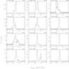 |
Fig. 1 Selected H2O maser spectra of U Her. The calendar date of the observation is indicated on the top left above each panel, and the TJD (JD-2 440 000.5) on the top right. |
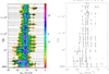 |
Fig. 2 Maser profiles of U Her as a function of time. Left: flux density versus Vlos as a function of time (FVt)-plot for U Her. Each horizontal dotted line indicates an observation (spectra taken within 4 days from each other were averaged). Data are resampled to a resolution of 0.3 km s−1 and only emission at levels ≥3σ and ≥l Jy is shown. The first spectrum in this plot was taken on 16 February 1990; JD = 2 447 938.5, TJD = 7938. Last spectrum shown is for 20 March 2011. Right: spectral components identified by the component fit of the single-dish spectra as listed in Tables A.1 and A.2 (see also Sect. 4.1.7). The component designations are given above the plot. Features which have been detected in adjacent spectra, are connected by solid lines. |
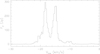 |
Fig. 3 Upper envelope spectrum for U Her; 1987–2015. |
3.2 Velocities and velocity ranges
In the following we define velocities and velocity ranges that we shall use in the analysis of the spectra. Only a short description is given here; for a detailed definition we refer to Paper II. The observed velocity ranges of the H2O maser emission are analysed in the frame of the ‘standard model’ for CSEs in evolved stars (Höfner & Olofsson 2018). This model assumes that the stars have radially symmetric outflowing winds, which form a spherical shell of dust and gas around them. The winds are accelerated so that the outflow velocity Vout is increasing with radial distance from the star before it reaches the final expansion velocity Vexp.
The velocity range over which H2O maser emission can be expected is constrained by the velocity ranges given by the OH maser and CO thermal emission. Both species are found beyond the typical H2O maser shells in regions where the wind acceleration has already ceased and the outflow velocity is constant (Höfner & Olofsson 2018). Then Vout ≤ Vexp and the observed H2O maser velocities Vlos are expected in the range V* − Vexp ≤ Vlos ≤ V* + Vexp.
We call the blue and red extremes of the observed H2O maser velocity range Vb and Vr, respectively. We use the detection-rate histogram for the determination of the observed maximum extent of the H2O maser velocity range ΔVlos = Vr − Vb (hereafter ‘maximum velocity range’) valid for the period of observations. This method gives accurate values (≈0.15 km s−1) for the maximum velocity range ΔVlos. In the case of spherical symmetry, we expect that the centre of the H2O maser velocity range is (Vb + Vr)/2 = V*.
One should note that the velocity range of individual observations and the maximum velocity range do vary with time because of two effects. First, for periods of time the outermost features may fall in brightness below the detection limit leading to an apparent variation of the observed velocity range. And second, maser emission might be excited out to larger or smaller distances for periods of time leading to a real increase or decrease of the maximum velocity range, respectively.
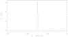 |
Fig. 4 Lower envelope spectrum for U Her; 1987–2015. |
 |
Fig. 5 Detection rate histogram for U Her; 1987–2015. |
4 U Her
U Her is a long-period variable AGB star at a distance of  (Table 1), based on the OH maser parallax measured by Vlemmings & van Langevelde (2007). We prefer the distance obtained by radio interferometry, because there is a large difference between the distances measured by the two astrometric satellites HIPPARCOS (
 ; van Leeuwen 2007, 2008) and Gaia EDR3 (
 ; Gaia Collaboration 2020, 2021), which may be caused by uncertainties introduced by stellar activity on optical parallaxes of nearby AGB stars (Chiavassa et al. 2018). Radial velocity determinations of UHer agree within ~0.5 km s−1 centred on V* = −15.0 km s−1. The final expansion velocity Vexp in the CSE can be as high as 20 km s−1 (Gottlieb et al. 2022), but here we use a more conservative value Vexp = 13.1 km s−1 (see Table 1).
The H2O maser of U Her was first detected in 1969 by Schwartz & Barrett (1970a,b) as a single feature at −15 km s−1 (their detection limit was ≈10 Jy). Until 1984 the maser was observed several times with detections in the velocity range −24 to −7 km s−1. The strongest peak was found either at −15 or −17 km s−1 (Engels et al. 1988, and references therein). Interfero-metric observations were made until the early time of our monitoring program with the VLA in 1983, 1988 and 1990 (Lane et al. 1987; Bowers & Johnston 1994; Colomer et al. 2000) and with MERLIN in 1985 (Yates & Cohen 1994). They found the masers to be located in an unevenly filled ring-like structure with typical inner and outer radii of ~10 and ~20 AU, respectively.
4.1 Single-dish data
4.1.1 Variations in brightness of the H2O maser profile
Our observations of U Her cover more than 28 yr, from March 1987 to October 2015. Contiguous monitoring was made between 1990 and 2011 with typically 5–6 observations per year. Depending on telescope (i.e. Effelsberg or Medicina), date of observation, resolution and integration time, the rms sensitivity of the observations was very inhomogeneous ranging from 0.1 to ~4 Jy. At the 0.3 km s−1 resolution used here, after mid-1991, with few exceptions all rms were <1.0 Jy. All 137 spectra taken are shown in Fig. C.1. Sample spectra showing typical profiles are given in Fig. 1.
A general view of the properties of the profile variations is given in the FVt-plot (Fig. 2, left panel) covering the years 1990–2011. The profile is usually dominated by emission in the velocity range −16 < Vlos < −14 km s−1 close to the stellar radial velocity V* = −15.0 km s−1, while in the outer parts of the profile (Vlos < −18 and > −14 km s−1) the emission is much weaker and at Vlos > −14 km s−1 appeared more or less regularly only around the maximum of the periodic stellar light variations. In the velocity range −18 < Vlos < −16 km s−1 emission was generally present but never dominating the profile; the peak at TJD = 8681 (29 February 1992) is caused by a spectral component at −18.2 km s−1, just outside this range (component D″ in Table 3). The plot clearly demonstrates that the maser emission is responding in strength to the periodic variability of the star. There is also an apparent broadening of the profile at regular time intervals, likewise connected to the pulsational period of the star. As shown in Sect. 4.1.3, the radio emission varies with the optical period but is lagging behind the optical one by about three months. In 1987 and 2015 the profiles were similar to those in 1990–2011 but the emission in the outer parts of the profile was not detected (Fig. C.1).
On top of the regular component of variability, non-regular flux density variations of individual maser features occurred, which led to strong profile variations over the years. This is exemplified by the upper envelope spectrum (Fig. 3), where the strongest feature is at −18.3 km s−1. This feature was strong for about 18 months between January 1991 (TJD ~8250) and July 1992 (TJD ~8800) (Figs. 1 and C.1). In the following, this period is referred to as the ‘1991/1992 peculiar phase’. The feature brightened again in autumn 1996 (TJD = 10352) for less than a year. No comparable brightenings were observed redwards of −14 km s−1. In contrast, the second prominent feature in the upper envelope spectrum at −15 km s−1 was permanently present, even in 1987 and 2015 prior to and after the phase of contiguous observations (see the lower envelope spectrum, Fig. 4). The emission close to the borders of the velocity range at Vlos < −20 and Vlos > −12 km s−1 (cf. also Fig. 1) is usually weak and becomes strong only occasionally. After 1996 (TJD ≳ 10 500) the blueshifted emission at velocities Vlos < −18 km s−1 faded away and after 2003 (TJD ≳ 13 000) it was not detected anymore by us. The long-term brightness variations are reflected in the FVt-plot (Fig. 2) as prominent asymmetry in the observed velocity range over time.
4.1.2 Variations of the H2O maser velocity range
The detection rate histogram (Fig. 5) confirms that the dominant spectral features occurred between −16 and −14 km s−1. It also shows that the total velocity range over which emission was detected is −23.3 < Vlos < −7.1 km s−1 (Table 1), which is symmetric with respect to the stellar radial velocity. The FVt-plot shows also that the width of the observed velocity range is varying. This is caused by the drop of the maser brightness at the weaker outer parts of the maser profile below the threshold of the FVt-plot (~l Jy) during the faint part of the stellar variability cycle.
The blue border of the H2O maser profile of U Her had been a point of discussion in the past, after emission had been detected at velocities ~2 km s−1 bluewards of the velocity range covered by the OH 1667 MHz maser emission and other molecular species (Engels et al. 1988; Bowers & Johnston 1994). However, given the final expansion velocity as obtained from more recent CO observations (see Table 1) the extreme blue H2O maser velocities at <−23 km s−1 (Engels et al. 1988), seen before the start of our observations are not ‘forbidden’ by the ‘standard model’ anymore, and instead asymmetries in the OH maser shell could be responsible for the lack of OH maser emission at very blue velocities.
4.1.3 Periodicity in the optical and radio light curves
As is evident from the FVt-plot (Fig. 2), the H2O maser variations of U Her show periodic behaviour, which is caused by the maser’s strong response to the stellar brightness variations.
We created the radio light curve of U Her using the integrated flux density determined over a fixed velocity interval encompassing all velocities at which maser emission was detected. The optical data (V-band) were taken from AAVSO6 for the years 1986–2015 encompassing the monitoring program and consisted of >2400 observations, while the radio data consisted of 137 observations. For both data sets a Fourier analysis was made to search for periodicity. The Lomb periodogram (Press et al. 1992) of the optical data showed a well defined period Popt = 405 ± 2 days, in agreement with the VizieR7 period of 406 days. The periodogram of the radio light curve confirmed the optical period (Prad = 407 days; Table 1), albeit with much larger uncertainties. To analyse the maser variations in relation to the optical variations of the star, we modelled in the following the optical and maser light curves by sine-waves with a common period and related the model light curves to each other.
4.1.4 The model for the optical light curve
The H2O maser variations are not in phase with the optical variations. It is well-established that for Mira variables they lag behind several weeks to months (Staley et al. 1994; Berulis et al. 1998; Shintani et al. 2008). To study this behaviour quantitatively we set the optical reference phase φs = 0 at the maximum of the optical model sine curve. These maxima are delayed in the mean by 25 ± 10 days relative to the observed optical maxima (∆φs = 0.06 ± 0.025 in units of phase). The delay is caused by the asymmetry of the optical light curve of U Her with a steeper rise to the maximum and a slower decline to the minimum and the scatter is due to the varying time differences between two real optical maxima. We found ΔT = 406 ± 15 days as the average time difference between two consecutive maxima, with extreme time differences of 374 and 426 days. The choice to link the optical phase to the model sine curve is therefore the only way to define an optical reference phase independent from the details of the optical light curve or the choice of the time interval over which the light curve is analysed. Adopting this approach, radio-optical phase lags can be compared between stars having different quality of the sampling of their optical light curves. Using for example the mean time difference between the observed optical maxima as reference is an alternative way to determine the delay ∆φs, but this method would be restricted to stars where the optical maxima are well observed. Our optical model light curve has a period Popt = 405 days and a reference epoch for maxima TJDmax = 6668 ± 3 days (Table 1).
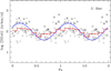 |
Fig. 6 U Her H2O maser light curve. Plotted are integrated flux densities S(tot) in the velocity range −24 < Vlos < −6 km s−1 in Jy km s−1 vs. optical phase φs. For better visualization the data are repeated for a second period. φs = 0 is defined as the time of maximum optical brightness. Datapoints marked by an asterisk (*) are from Eſſelsberg, the plusses (+) are Medicina data. Overplotted are average integrated flux densities in phase bins of 0.1 (red), and a sine curve (blue) which was obtained by a fit to the 1990–2011 radio measurements with a period of Popt = 405 days. The sine curve is delayed by ϕlag = 0.16, i.e. by 64 days with respect to the optical maximum. |
4.1.5 Phase lag between optical and radio light curve
The lag of the radio light curve relative to the optical one was determined with the fit of a sine curve to the radio data using the optical period, and the amplitude as free parameter. Only radio observations during the continuous monitoring between 1990 and 2011 were used, and observations taken within 3 days were averaged. The final data-set to determine the radio light curve consisted of 125 maser spectra. The resulting lag of ϕlag = 0.16 (Table 1) is only weakly depending on the choice of the amplitude. The radio light curve is shown in Fig. 6 as a function of the optical phase φs. It is immediately clear that the scatter in integrated flux densities S (tot) is large for any particular phase, indicating that the luminosity variations of the star can explain only part of the maser variability seen. To visualise the periodic component of the variations we overplotted a binned light curve (average integrated fluxes in bins of 0.1 in phase) and the sine curve obtained from the fit using the optical period. In Fig. 6 the integrated flux densities S (tot) obtained with the Effelsberg telescope appear to be systematically brighter than those obtained with the Medicina telescope. This is a selection effect caused by the general brightness decrease of U Her’s maser light curve (see Fig. 7) and the limitation of the Effelsberg observations to the first years. This leads to a fraction of observations during bright maser phases being significantly higher for the Effelsberg than for the Medicina radio telescope.
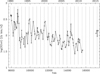 |
Fig. 7 U Her H2O maser light curve, showing the total flux (integrated between Vlos −24 km s−1 and −6 km s−1) as a function of TJD. The vertical dashed lines indicate the (modelled) optical maxima with P = 405 days. |
4.1.6 Long-term radio light curve
In addition to the periodic maser brightness variations, additional brightness changes are seen also on timescales shorter and longer than the stellar period. In Fig. 7 we plot the total flux of the U Her H2O maser as a function of time between 1990 and 2015. As is evident also here, the variations in the maser emission follow the optical variations of the star, indicated by the dashed lines that mark the TJD of the (modelled) stellar maxima (see Sect. 4.1.4). Although the dominance of the emission in the −16 to −14 km s−1 velocity interval after 1992 suggests some long-term continuity, this continuity is restricted to velocities and not to brightness levels. The radio light curve shown in Fig. 7 indicates a clear decrease by a factor of 4 of the average brightness level between 1990 (5 (tot) ~ 200 Jy km s−1) and 2011 (5 (tot) ~ 50 Jy km s−1). In 2015 the brightness level had increased again to (5 (tot) ~ 125 Jy km s−1), while in April 1984 the total flux was 185 Jy km s−1 (Engels et al. 1988). The strong emission in February 1992 during the ‘1991/1992 peculiar phase’ (see Sect. 4.1.1) could have been a burst. After this phase emissions at Vlos < −17 km s−1 dropped sharply and the total flux went through a weak phase lasting until 1995, when a brightness increase of the −15.5 km s−1 feature brought the total flux back to a level following the long-term decline of the average brightness.
The 1990–2011 long-term brightness decrease is not uniform over the velocity range, but due to a systematic brightness decrease of the emission that is blueshifted with respect to the stellar velocity (V* = −15 km s−1). As shown in Fig. 8 the ratio 5 (blue)/5 (red) between the blue- and redshifted total flux is continuously decreasing between ~1992 and ~2007. During the ‘1991/1992 peculiar phase’ 5 (blue) was ~15 times stronger than 5 (red), while in 2007/2008 the ratio could be as small as ~0.5. The strength of the redshifted emission in the period 2007 – 2011 (TJD > 13 500) appears to be due to the shift of the peak emission in the −16 to −14 km s−1 velocity interval by < 1 km s−1 to the red (see the FVt-diagram, Fig. 2, left). The choice of the stellar radial velocity influences the ratio quantitatively but its trend remains for any radial velocity within the dominant −16 to −14 km s−1 interval. The 5 (blue)/5 (red) ratio and its variation indicate an asymmetry of the excitation conditions in the front part of the H2O maser shell of U Her, where the blueshifted emission comes from, compared to the rear part, where the redshifted emission originates.
The radio light curve (Fig. 7) shows three rather bright maxima compared to the times before and after. They are the possible burst in the ‘1991/1992 peculiar phase’ (peak emission at TJD = 8682), the maximum in 2000 (peak on TJD = 11 640) and the maximum in 2007 (peak on TJD = 14 389). We consider them as short-term fluctuations rather than as evidence of ‘super-periodicity’, because the time intervals between the peaks with a duration of 6.8 and 7.3 stellar cycles do not match. The next maximum would have been expected in April-September 2015. We have observations in this time interval, but no information on the brightness levels before and after. It is therefore not possible to decide if the brightness levels observed in 2015 belong to a local maximum or are part of a general increase of the brightnesses.
Besides our monitoring program, U Her’s H2O maser has been observed with single-dish telescopes only occasionally by other groups. Excluding the ‘1991/1992 peculiar phase’, the strongest maser feature was consistently reported at approximately −14.5 km s−1 by Comoretto et al. (1990) for March 1987, by Kim et al. (2010) for June 2009, and by Neufeld et al. (2017) for May 2016. In 1991 the strongest peaks were at −16 (Takaba et al. 1994) and −19 km s−1 (Takaba et al. 2001) in accordance with our observations.
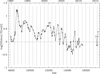 |
Fig. 8 Ratio S (blue)/5 (red) of the U Her H2O maser emission, of the Vlos < −15 km s−1 [S (blue)] and > −15 km s−1 [S (red)] part of the maser velocity range with respect to the stellar velocity, as a function of TJD. The vertical dashed lines indicate the (modelled) optical maxima with P = 405 days. |
4.1.7 Velocity variations of individual H2O maser features
In addition to the regular periodic and long-term brightness variations of U Her’s H2O maser emission, also small changes in velocity of the maser features are apparent in the FVt-plot (Fig. 2). For their analysis we decomposed the H2O maser spectra 1987–2015 into separate features by fitting multiple Gaussian line profiles. The details of the fitting technique are described in Paper I. These maser features can be traced over some period of time in several consecutive spectra, fade away, and may reappear at later times perhaps with a slightly different velocity. As in the semiregular variable stars (Papers I and II), the full width at half maximum (FWHM) of strong features (visible as distinct peaks in the spectra) is ~1 km s−1, and therefore features with FWHM ~ 2 km s−1 are most probably blends. We assume that maser features in adjacent (in time) spectra with velocity differences <0.5 km s−1 belong to a unique emission region in the H2O maser shell, which persisted over this period of time (i.e. the time between the two observations) and varied in intensity.
For accounting purposes all spectral features were grouped according to their velocities into maser spectral components. The assignment of the features to the spectral components in the four velocity intervals (< −18, −18 to −16, −16 to −14 and > −14 km s−1 as introduced in Sect. 4.1.1) is discussed in Appendix A. Tables A.1 and A.2 list the spectral features identified by the fitting procedure and their assignments.
The spectral components are labeled with capital letters A, B, … M in order of increasing velocity Vlos. Their labeling is synchronised with the labels of the spatial components (to be introduced in Sect. 4.2.1), so that corresponding spectral and spatial components share the same label. Due to strong blending in velocity space, in each of the four velocity ranges only few (one to four) spectral components could be defined. In total we identified eleven spectral components. Not all spatial components could be identified in the single-dish spectra, especially not the fainter ones, and therefore there are no spectral components matching the spatial components A1, F1+F2, H1+H2, and J1+J2 (cf. Table 3 in Sect. 4.2.1). Two spectral components (D at approximately −18.5 km s−1 and G at approximately −15.0 km s−1) are obvious blends with velocity separations less than the FWHM of the features. In Tables A.1 and A.2 the subcomponents making up the spectral components D and G were labeled D′, D″ and G′, G″ respectively.
The maser spectral components identified in individual spectra (Tables A.1 and A.2) are graphically displayed in Fig. 2 (right panel), where it can be compared directly with the FVt-plot. Often, changes of the spectral component peak velocities Vlos (taken from Tables A.1–A.2) in all four velocity ranges occur on timescales of many months by more than 0.5 km s−1, although not in a systematic way. An example are the peak velocities of spectral component G′ in 2007–2011 (TJD ~ 14 000) with velocities −16.0 ≤ Vlos ≤ −14.8. We interpret the meandering of the velocities as a superposition of blended maser features varying in brightness asynchronously and coming perhaps over some time from different locations.
The interpretation of the short-term velocity variations is less ambiguous in the > −14 km s−1 velocity range, where fewer spectral features are apparent and therefore blending is less of a problem. Component I shows evidence for blending between 1990 and 1996 (~ 7900 < TJD <~ 10200) with peak velocities varying back and forth by almost 1 km s−1 (−13.7 to −12.7 km s−1; see Table A.2), while the velocity remained almost constant at −12.9 km s−1 thereafter until TJD ~ 14500. It then reappeared at the same velocity in 2015. Component K has a peak velocity of ~ −11 km s−1 and was detectable only after 1994 (TJD > 9750), also without significant velocity variations. Component L was seen only in two epochs 1990–1992 (TJD < 8900) at −10.2 km s−1 and 2007–2010 (14000 < TJD < 15300) at−-9.7 km s−1, and it is unclear if the emissions in these two epochs are related to each other. Finally, component M at ~ −8 was only seen at the beginning of the monitoring program, in parallel to component L (1990–1992), while the maser emission in U Her was strong over the full profile. There were too few appearances to draw conclusions on its velocity variations.
In the velocity range covered by components I to M we would expect shifts of increasing velocity (components becoming redder), if the emission regions would persist and move with the expanding CSE. This is not the case here, and so the emission of these components must have come from different emission clouds in the course of the monitoring period. The absence of long-term velocity shifts of the spectral components will be discussed further in Sect. 4.5.
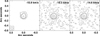 |
Fig. 9 Sample H2O maser images of U Her from February 1990 covering the velocity range between −16 and −14 km s−1 with the strongest emission. The synthesised FWHM beam size (major axis: 0.″09; minor axis: 0.″08; position angle of the major axis: 71◦) is shown in the left panel (−15.9 km s−1). The images are oriented along right ascension and declination and the angular scales are relative to the position α = 16h25m47s.39, δ = +18◦ 53′ 32.9″ (J2000). Brightness contours are −0.25 (dashed contour), 0.25, 2.5, 5, 50, and 150 Jy per beam area (1.4 10−13 sr). |
4.2 Interferometric data
The VLA observations of the H2O masers in U Her were made with the aim to identify the emission sites in the CSE and breaking the spatial degeneracy in the single-dish data. Due to the limited spatial resolution this was only partially successful. The size of the emission sites is not specified a priori, but we refer to the most compact gas clumps hosting maser emission as ‘maser clouds’. The data analysis of the images yields maser spatial components, which in general will be superpositions of several maser clouds close to each other in space as well as in velocity.
4.2.1 Spatial component identification
The VLA interferometric data consist of one data cube for each of the four epochs, containing 63 channel maps each. The maps are separated in velocity by 0.658 km s−1. An example is given in Fig. 9 where maps of the 3 channels with the strongest emission seen in the first VLA epoch (February 1990) are shown. The sensitivities measured in a line-free channel were 12–21 mJy beam−1.
In order to single out maser components the data cubes were analysed within AIPS8 in a three step process. First, the individual channel maps were analysed one by one by fitting multiple 2D Gaussians, then spatial components were identified by comparing the fit results in neighbouring channel maps, and finally these components were verified in velocity space. The details of this analysis are described in paper I.
About 12 spatial maser components were identified in each VLA observing epoch. These components are listed in Table 3, which gives the spatial component (Spat), the VLA observing epoch, the Vlos and peak flux density Sp of the spatial components identified, the spatial offsets (Xoff and Yoff) from the adopted map centre (defined in Sect. 4.2.2) and the associated (single-dish) spectral component (Spec) from Tables A.1 and A.2. Spectral component B had different spatial counterparts in 1990 and 1991. Spectral component D′ is not listed as it appeared only after 1990– 1992. Spatial component G1 is likely of composite nature, as the corresponding spectral component G is according to our analysis of the spectral profiles made up by two components (G′ and G″ in Table A.2).
For the epoch June 1990 the components can be compared to those found by Colomer et al. (2000), who used the VLA to observe U Her one day apart from our observation. As in the case of RX Boo (see paper I) they found about the same number of components (13 vs. 12). However, their components are spread over a smaller velocity range of −18.3 ≤ Vlos ≤ −10.2 km s−1, because they did not detect the faint components B1 (Vlos = −21.2 km s−1, Sν = 0.1 Jy) and M1 (Vlos = −8.0 km s−1, Sν = 0.2 Jy) (cf. Table 3). Our strongest spatial component in June 1990, G1 (Vlos = −15.0 km s−1) is split by the 3-dimensional Gaussian fitting program of Colomer et al. into three spatial components in the velocity range −15.3 < Vlos < −14.6 km s−1. This corroborates our conclusion that G1 is of composite nature. Common components in both June 1990 maps are present outside the very crowded main velocity range −16 < Vlos < −14 km s−1, if flux densities surpassed 1 Jy, whereas weaker spatial components were not recognised by the fitting program of Colomer et al.. As discussed in Paper I, the two fitting methods lead to different results for weaker components and regions of high spatial blending. The overall spatial distributions of both maps is however similar, and so the projected angular shell sizes are similar.
4.2.2 Alignment of the maps
The maps taken between 1990 and 1992 were aligned to a common origin using spatial components present over two or more observing epochs and assuming that the components are located in a ring-like structure around the star. Matched components are given a common designation in Table 3. For example at Vlos ≈ −20.0 km s−1 the strong C1 spatial component seen in October 1991, is identified in February 1990 and December 1992 as a weak component, while other spatial components (C2, C3) identified at (or close to) this velocity are clearly coming from different parts of the shell. As in the case of RX Boo (Paper I), the 1990 maps had many components in common, while components in 1991 and 1992 were difficult to identify with components seen in the other years. The identification was further complicated by the poor east-west resolution in October 1991, and the ‘1991/1992 peculiar phase’, in which the masers were at that time. As discussed in Sect. 4.1.1, the maser emission at Vlos ≤ −18 km s−1 was prominent around the turn of the year 1991/1992, while in other epochs this emission was relatively weak and emission from the −16 < Vlos < −14 km s−1 velocity range prevailed. In October 1991 spatial components B2 and C1 were strongest (Table 3), while the strongest component during the other three epochs (G1) could not be identified. The components used to align the December 1992 map with the maps from 1990 were D1 and G1, which were strong in both years. C1 and D2 were used to align the October 1991 map. After alignment these components scattered in position by ≤12 mas.
A plot of all spatial components on the sky relative to a common origin as given in Table 3 is shown in Fig. 109. The distribution of the components suggests a ring-like structure. To find the most likely position of the star, a circle was fitted according to a least-squares method to all components having radial velocities between −18 and −14 km s−1. They were considered as being likely ‘tangential components’, able to outline the ring-like structure of the projected shell. The fit was carried out without weights and the centre of the circle was used as our best guess for the stellar position, and as common origin of the plot and of the component offsets in Table 3. The best fit gave a radius for the circle of 57 mas (~15 AU).
Spatial coincidences among other components were searched for in the aligned maps. Coincident spatial components detected in different epochs were given a common label. After subtraction of coincident components we ended up with 28 different spatial components (hereafter ‘merged spatial components’) of which half were present in at least two maps. Positional deviations between maps were ≲15 mas, although in a few ambiguous cases we accepted as coincidences also components with deviations up to 45 mas (cf. B1, H2, J1 in Table 3). The number of merged spatial components found and the accuracies in velocities and positions are very similar to the results obtained for the SRV RX Boo in Paper I.
Spatial (‘Spat’) and spectral (‘Spec’) components of U Her 1990–1992.
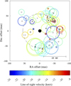 |
Fig. 10 All the spatial components of U Her listed in Table 3 plotted on the sky. Each component is represented by a symbol surrounded by a circle with a diameter d depending on flux density Sν: d = 8 (log Sν + 1.3). The dates are represented by different symbols: Feb. 90 by small circles; Jun. 90 by asterisks; Oct. 91 by plus signs; Dec. 92 by crosses. The circles around the components are colour coded according to the Vlos of the component (see the scale below the map). The dashed circle with a radius of 57 mas has been obtained from a fit to the components with velocities −18 < Vlos < −14 km s−1 (see text) and the origin of the plot has been moved to the centre of this circle. The filled black circle at the centre symbolises the central star with a diameter of 10.65 mas (van Belle et al. 1996). |
4.2.3 Cross correlation of single-dish and interferometric data 1990–1992
The assignment in Table 3 of spectral components identified in Sect. 4.1.7 to the spatial components identified in Sect. 4.2.1 was made using the velocities in common. Spatial component A1 detected in October 1991 at −23.8 km s−1 with a peak flux density of 0.4 Jy was not present in any of our spectra. Its velocity is lower by 0.5 km s−1 than the blue border of the H2O maser velocity range that we determined in Sect. 4.1.2 from the single-dish spectra. Due to blending in velocity space also other weaker spatial components (≤10 Jy: spatial components F, H, J) could not be assigned to individual spectral components. An exception are the spatial components M1 and M2 at approximately −8 km s−1 in the extreme red part of the velocity range. Their emission could be detected in the spectra due to absence of stronger maser emission at neighboring velocities. The brighter spectral components D′ and K at −18.9 ± 0.2 and −10.8 ± 0.3 km s−1 respectively (see Tables A.1 and A.2) were not seen in our spectra before 1993. Accordingly, spectral component D′ was not assigned to any spatial component, and spectral component K is absent from Table 3 because no emission was seen at the corresponding velocities in the VLA maps 1990 – 1992. Spatial component G1 is a blend of two emission sites, which could be identified as subcomponents G′ and G″ of spectral component G in the single-dish spectra due to their superior velocity resolution.
For brighter spatial/spectral components the cross-correlation was not unambiguous at several velocities, due to blending in velocity and position. One case is spectral component B with peak velocities −21.1 ± 0.5 km s−1, which was the strongest in the maser profile probably only for a couple of days during the ‘1991/1992 peculiar phase’. The VLA map of 20 October 1991 was made close to the maximum of this phase and the emission was detected in the east part of the shell (spatial component B2 at −22.0 km s−1). The peak velocity of B2 is 1.4 km s−1 lower than the peak velocity −20.6 km s−1 of the spectral component B measured 6 and 13 days later (cf. Table A.1). Such a large velocity difference between spatial and spectral components was not seen by any other component, and may indicate the presence of brief emission bursts on the timescales of many days.
The peculiarity of the ‘1991/1992 peculiar phase’ is evident also from the result that in 1990 the spectral component B maser emission came from a different part of the H2O maser shell (spatial component B1 in the north-east part of the shell). There was no emission at corresponding velocities in December 1992. In parallel to spectral component B also component C reached a maximum between October 1991 and April 1992 (see Table A.1). This emission was located in the south-west of the shell, and in this case emission from this part at that velocity was seen also in the maps from 1990 and 1992 (spatial component C1).
The cross-correlation is also complex for velocities Vlos ≥ −18 km s−1. Spatial components D1 and D2 (Vlos ~ −18 km s−1, velocity difference ≈ 0.2 km s−1) cannot be separated in the single-dish spectra, and coincide in velocity with spectral component D″. Spectral component D′ was not prominent in 1990–1992. Spatial component E3 is the strongest component among five in the velocity range −17.2 < Vlos < −16.6 km s−1. It was not identified in the spectra of 1990, but was detected as spectral component E in 1991 and 1992. As E3 comes in velocity space from close to the brighter spectral component D″, it was not distinguished in the 1990 spectra because of blending.
In the −16 < Vlos < −14 km s−1 range the dominating spectral feature G, composed of G′ and G″ (velocity separation in 1990: 0.7 km s−1), was identified spatially as one component G1, caused by the insufficient spectral resolution of the VLA data (~0.7 km s−1). The maps show however, that both spectral features came from the same region in the southern part of the shell. Spatial component G1 was detected in 1990 as well as in December 1992 and was therefore a dominant emission region over a time range of at least 3 yr, except for a few months in 1991/1992.
At velocities ≥ −14.5 km s−1 of the nine different spatial components listed in Table 3 only three (I1, L1, and M1 from the 1990 maps) could be distinguished also in the spectra (Table A.2). The velocities corresponding to spatial components H1 and H2 (Vlos ≈ −14.1 km s−1) are strongly blended in the spectra by the dominating spectral component G″. In the 1991 and 1992 maps spatial components at larger velocities (Vlos > −14 km s−1) were eitherabsent(October1991)orextremelyweak(0.1 Jy).
4.3 An H2O maser shell model for U Her
4.3.1 The projected structure
The distribution of all spatial components observed in U Her 1990-1992(Fig. 10)is best described as an incomplete ring with most components located in the half of the ring between position angles 170 and 350◦ counting from North over East.
Following the analysis and discussion of the location of the H2O masers in the circumstellar envelope of the semiregular variable RX Boo (Paper I), we assume that the H2O masers are embedded in an isotropically expanding envelope. In this case, the relationship between the Vlos of the maser spatial components relative to that of the star and their projected distances rp from the star is given by
 (1)
(1)
where r is the radial distance, and Vout is the outflow velocity of the components, and V* is the radial velocity of the star.
Using V* = −15.0 km s−1 (Table 1), we plotted in Fig. 11 the relative line-of-sight velocity |Vlos − V*| in absolute values of all 48 spatial components against their projected distance rp. |Vlos − V*| and rp were calculated using Vlos-, Xoff-, Yoff-values fromTable3. For a shell-like distribution of the masers we expect, according to Eq. (1), elliptical inner and outer boundaries for their locations in Fig. 11. Unlike in the corresponding diagram of RX Boo (Paper I), there is no sharp inner boundary, but an outer boundary can be defined, by fitting a quarter of an ellipse to the six outer maser components marked by surrounding circles in Fig. 11, using the ‘least-squares method’. From this fit we conclude that the outflow velocity in the envelope of U Her at ~24 AU from the star is about 10 km s−1.
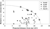 |
Fig. 11 Relative line-of-sight velocity |Vlos − V*| versus projected distance rp for all spatial components of U Her from Table 3 identified in the four epochs. The six outer points surrounded by circles were used for the fit with a quart ellipse. |
4.3.2 The three-dimensional shell structure
As in Paper I we assume that the outflow velocity law is exponential in nature and is leading asymptotically to the final expansion velocity, Vexp
![Mathematical equation: ${V_{{\rm{out }}}}(r) = {V_{\exp }}\left\{ {1 - \exp \left[ { - k\left( {r - {r_0}} \right)} \right]} \right\}$](/articles/aa/full_html/2024/06/aa48567-23/aa48567-23-eq7.png) (2)
(2)
where k is a scaling factor and r0 is a radial offset.
Equation (2) contains three constant parameters (Vexp, k and r0) and in order to find plausible values for them we need to estimate the coordinate values for three points on the outflow law. For the value of Vexp (the outflow velocity at r = ∞) we adopted Vexp = 13.1 km s−1 (Table 1). Based on the fit of the ellipse shown in Fig. 11 to determine an outer boundary of the shell, we adopted an outflow velocity of 9.6 km s-1 at a distance of 23.9 AU from the star. We also assumed that the outflow velocity at the photosphere r0 = 1.4 AU is Vout = 0 km s−1.
Therefore, the value of the parameter k can be determined from the condition that the stellar wind passes through the position (r1, V1) = (23.9, 9.6). Using
 (3)
(3)
we obtain k = 0.059 AU−1.
For the case of non-tangential movements of maser components, the model allows one to calculate the observed Vlos and projected distances rp from the equations
 (4)
(4)
and
 (5)
(5)
where θ is the aspect angle between the normal to the line of sight and the radius from the star to the maser. The aspect angle is −90° ≤ θ ≤ 0° for Vlos − V* < 0 km s−1 and viceversa.
Combining Eqs. (2), (4), and (5) gives a relation, which uniquely determines the distance r of the maser cloud from the star for the time of the distance measurement, using the adopted outflow law and the observed quantities (Vlos − V*) and rp
![Mathematical equation: ${V_{{\rm{los }}}} = {V_{\exp }}\left\{ {1 - \exp \left[ { - k\left( {r - {r_0}} \right)} \right]} \right\} \cdot \sqrt {1 - {{\left( {{r_{\rm{p}}}/r} \right)}^2}} + {V_*}.$](/articles/aa/full_html/2024/06/aa48567-23/aa48567-23-eq11.png) (6)
(6)
In Fig. 12, the adopted outflow velocity law with the parameters k = 0.059 AU−1, r0 = 1.4 AU and Vexp = 13.1 km s−1 is shown graphically, together with the radial distances r of the maser spatial components calculated with Eq. (6). The projected distances  used for these calculations were averages over the epochs in which the components were detected (Table 3). The uncertainties in positions and velocities lead to errors in the radial distances r of a few AU, and so their locations on the velocity curve mainly delineate the typical distance range of the maser components. The main conclusion is that the maser shell is primarily located between ~11 and ~25 AU. The outflow velocity within these boundaries increases from 5.6 to 9.8 km s−1. The maser components outside this shell (>25 AU) are the spatial components A1 and M1 which have Vlos at the extreme ends of the observed velocity range, and have the largest outflow velocities Vout. The component inside this shell is the tangential component G2 with Vlos − V* = −0.1 km s−1 close to the line-of-sight toward the star itself. The two outliers at r > 25 AU with flux densities < 1 Jy indicate that weak and short-lived maser activity can occur outside the shell delineated by the strong maser components. The same is true for the regions inside the inner boundary of the shell, in which the masers are usually suppressed because there the acceleration of the wind is relatively high. Due to projection effects the shell radius (r = 15 AU), derived from the spatial distribution of the maser components on the sky (Fig. 10), is ~80% of the mean radius of the shell (r ~ 18 AU) given by the midpoint between inner and outer boundary of the 3D model.
The 3D distribution of the merged maser spatial components and their associated velocities is shown in Fig. 13 as seen from three different directions: on the sky (a), ‘from the side’ (b) and ‘from above’ (c). The dominance of tangential masers is seen clearly in all three diagrams. In panel (c) there is a scarcity of (redshifted) components seen on the backside of the shell. This is also evident in the FVt-plot (Fig. 2, left), where there is less emission at redshifted velocities, and in Fig. 8 where the blueshifted integrated emission prevailed between 1991 and 2007. However, one should keep in mind that an observer seeing U Her from direc-tions deviating considerably from the geocentric one would see a different set of maser components, because a maser beams in a preferred direction, which is governed by the direction of greatest elongation of the maser cloud. Therefore, Fig. 13 is merely showing the three-dimensional positions of the maser components that we see from Earth. Of course a similar situation occurs for our present point of observation: there may be maser spots that we do not see because their emission may happen to be beamed in the wrong direction from our vantage point.
Having adopted an outflow law it is of interest to investigate the associated timescale for the gas to travel through the maser shell. Therefore, we integrated the function  , where Vout is described by Eq. (2), along the radius r between the shell boundaries. We find that it takes ~8.5 yr for gas to travel through the shell (11–25 AU), where most of the H2O masers reside.
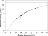 |
Fig. 12 Model outflow velocity for U Her as a function of the distance from the star. It approaches the final expansion velocity (horizontal straight line) asymptotically. The dots along the curve give the radial distances and outflow velocities of the 28 merged spatial components (see text). |
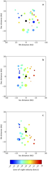 |
Fig. 13 Three-dimensional distribution of the U Her merged maser spatial components and their associated velocities according to the outflow velocity law given by Eq. (2). The distribution is seen from three cardinal directions: on the sky (a), ‘from the side’ (b) and ‘from above’ (c). In (b) and (c) the observer is to the left. The maser components are represented by filled circles with colours according to their Vlos (see scale at bottom). Their diameters are proportional to the logarithm of their flux density. The central star is symbolised by a black circle at (0,0). |
4.4 Other H2O maser shell observations of U Her
4.4.1 Maser shell sizes
Our shell model can be directly compared to the results of the contemporaneous 22 GHz VLA observations of Colomer et al. (2000) from June 1990 discussed in Sect. 4.2.1. Using a 3D fitting program they advocate a thick maser shell with an inner radius of 45 mas (~12 AU) and an outer radius of 70 mas (~19 AU), in which the molecules flow outwards with a velocity of ~6 km s−1. A comparison with our model expansion velocity law (Fig. 12) shows that their shell boundaries delineate a narrow 7 AU-wide shell in the central part of our shell model covering the strongest spatial maser components. The average radius of this shell is ~15.5 AU compared to ~18 AU, the average radius of our shell model. The two independent analyses highlight the uncertainties in the determination of the boundaries, with the shell boundaries for 1990 of Colomer et al. being a conservative estimate.
After our VLA observations 1990–1992, the H2O maser emission of U Her was mapped several times and these observations can be used to search for variations in the spatial distribution of the masers over a longer time range. Interferometric observations with better spatial resolution than achievable with the VLA were made with MERLIN 1994, 2000 and 2001 (Bains et al. 2003; Richards et al. 2012), and with the VLBA in 1995 (Marvel 1996). They confirm the overall ring-like geometry of the H2O maser shell. However, the boundaries of this shell determined from the different observations are not well defined. The most compelling determination is by Richards et al. (2012) who, for the epochs 2000 and 2001, found projected inner and outer radii of 10 and 40 AU, respectively. While the inner radius is compatible with the inner boundary determined here and by Colomer et al. (2000), the outer radius is significantly larger. However, the outer shell at radii >30 AU was only sparsely populated by maser components in 2000/2001 (Richards et al. 2012), and these were not detected 1990–1992. The decrease in brightness of the maser emission with radial distance makes the determination of the outer shell boundary much more dependent on instrumental sensitivity compared to the inner boundary. The conclusion from all H2O maser shell observations available is that the H2O masers are located in a shell within the expanding spherical wind of U Her with most of the sites with stronger emission located at a radial distance of about 15–20 AU. Nevertheless, VLBA observations by Vlemmings et al. (2002a, 2005) challenged the characterization of U Her’s H2O maser shell as a persistent ring-like distribution of distinct emission regions.
4.4.2 Constraints on shell geometry due to spatial resolution effects
To study magnetic field strengths in the CSE of U Her, 22 GHz observations with the VLBA were made on 13 December 1998 by Vlemmings et al. (2002a) and on 20 April 2003 by Vlemmings et al. (2005) with an average beam width of 0.5 mas. They noted a significant change in spectrum and spatial distribution between the two observations. The spatial features detected in 1998 (optical phase φs = 0.44) were at velocities −19.3 to −17.6 (likely part of our spectral components D′ and D″), while in 2003 (φs = 0.97) they detected features at −15.9 to −14.5 (G′ and G″). Our single-dish spectra taken close to their observations (12 December 1998 and 2 April 2003, see Fig. C.1) show a stronger profile change only in the red wing (> −14 km s−1), but not at the velocities with VLBA detections by Vlemmings et al.. During both epochs spectral components G′ and G″ were strongest, while D′+D″ was 2–3 times weaker. It is therefore conceivable that the spatial distribution as such did not change significantly between the two epochs, but the sizes of the spatial components did, leading to different components being resolved out by the VLBA in the two epochs. This explanation is corroborated by the failure of Imai et al. (1997b) to detect U Her’s H2O maser emission in 1994/1995 during a VLBI experiment (resolution 2.1 mas), indicating that the dominating spectral components G′ and G″ had significantly larger sizes. Richards et al. (2011) give typical sizes 2–5 AU (8– 19 mas) for H2O maser clouds of U Her, and so losses of spatial features due to the largest recoverable scale for imaging with the VLBA are plausible.
4.4.3 No evidence for maser amplification by stellar emission in 2001
Vlemmings et al. (2002b) mapped the maser on 20 May 2001 with MERLIN (beam size ≤30 mas), when the strongest spectral maser feature was present at −15.6 km s−1 (spectral component G′, see Table A.2 and Fig. C.1). These authors found the position of the feature to match with the location of the star at this epoch, determined using own and HIPPARCOS proper motion measurements of U Her, and argued that the maser feature is amplified by the stellar radiation in the background. They note that this result would place the star not in the centre but on the ring-like distribution of the maser spots.
In the monitoring data we find no evidence for extraordinary amplification of the G′ component. If the G′ component would have moved as part of the stellar wind in radial direction within the line-of-sight to the star, a systematic blueshift of its velocity Vlos over time is expected, which is not observed. Alternatively, if G′ would have moved in tangential direction the stellar amplification would be only a temporary effect during the time of eclipse. Adopting a U Her maser cloud size of 2–5 AU (Richards et al. 2011), a stellar diameter of 2.8 AU (van Belle et al. 1996; Ragland et al. 2006) and a velocity of ~7 km s−1 perpendicular to the line-of-sight (see Fig. 12) leads to a duration of the eclipse of several years. Therefore, a monitoring program of such an eclipsing event is expected to observe a temporary year-long flare of the emission on top on the regular maser variations. The occurrence of such a flare of the G′ emission can be definitely ruled out in the years around 2001.
Using the stellar position and proper motion given by Gaia EDR3 we recalculated the position of the star for the MERLIN observation of Vlemmings et al. (2002b) and found an offset of the position of the maser spot from the star of Δα = −37.4 mas and Δδ = 0.3 mas, which places the maser spot ~ 10 AU west from the star and at the inner boundary of the H2O maser shell as determined earlier.
Based on the lack of brightness and velocity variations of spectral component G′, which could be related to an eclipse event, and based on the stellar position in 2001 according to recent Gaia astrometry, we conclude that the assumption of the stellar position close to the centre of the ring-like distribution of spatial components, as made in Sect. 4.2.2, is still a valid approach. The location of the H2O masers in a shell within the spherically expanding stellar wind therefore remains the most plausible geometric configuration.
4.5 Lifetime of emission regions
The analysis of the line profile variations in Sect. 4.1.7 found the velocities of the spectral components remarkably constant over the monitoring period with only small shifts back and forth on timescales of months. The small shifts were assumed to be caused by blending caused by different maser clouds with similar velocities and unrelated brightness fluctuations. They may reflect the asynchronous formation and dissolution of contributing maser clouds or a variation of excitation conditions on these timescales.
We also found that some less blended spectral components could be followed without significant variations in velocity over longer time ranges. An example is component K, which could be detected continuously for 5 yr (March 1995–April 2000; TJD = 9790–11 640; see Fig. 2, and Table A.2) at -10.9 ± 0.2 km s−1, so with a rather small velocity dispersion. Later it reappeared frequently close to the maxima of the stellar variability cycle. If this emission component comes from an individual maser cloud, one has to conclude that UHer’s H2O maser shell can host individual clouds with a range of lifetimes of 0.5 to many years. Alternatively, short-living clouds would have to appear regularly with always similar Vlos.
In the first case of a long-living maser cloud, which moves within the expanding CSE, systematic shifts of the projected velocity Vlos are expected, while the cloud is accelerated outward. This is not seen in any of the spectral components, and so the second case must apply and their emission must come from different short-living spatial components in the course of the monitoring period.
4.5.1 Maser cloud lifetime constraints
We now use the absence of systematic velocity shifts to derive upper limits for the lifetime of individual maser clouds. For the outflow velocity curve shown in Fig. 12, we found in Sect. 4.3.2 a crossing time of ~8.5 yr for a mass element moving radially through the H2O maser shell with inner and outer boundaries of 11 and 25 AU, and with an increase of its outflow velocity from 5.6 to 9.8 km s−1. Moving in the line-of-sight, such a hypothetical mass element showing maser emission all the time would show an acceleration of a = 0.5 km s−1yr−1.
A maser cloud observed in two epochs with a time difference Δt and moving along a straight trajectory in the shell with an angle θ with respect to the plane of the sky will experience a shift in velocity δVlos = δVout(r) • sin θ (cf. Eq. (4)), with δVout(r) the increase of the outflow velocity. For simplicity, we approximate the acceleration within the H2O maser shell with the average velocity increase a = 0.5 km s−1yr−1, that is δVout(r) = a • Δt leading to the relation
 (7)
(7)
In the following, we adopt a conservative value |δVlos| < 0.5 km s−1 for recognisable velocity shifts due to participation in the stellar outflow of any of U Her’s spectral components. For a given time interval Δt, only maser components with an aspect angle obeying
 (8)
(8)
would not have been detected as having a drifting los velocity. A special case of Eq. (8) is a tangential movement of the maser clouds (θ ≈ 0), where a constant velocity Vlos (i.e. δVlos ≈ 0) can be expected for maser clouds traceable over long time intervals. Equation (4) demands that in this case Vlos ≈ V*. Allowing an uncertainty of 0.5 km s−1 for the stellar radial velocity V* = −15.0 km s−1, such a tangential movement would be able to explain the absence of velocity shifts for spectral components G′ (∽−15.5 km s−1) and G″ ( 14.5 km s−1). However, as our monitoring period is longer than the crossing time in U Her’s H2O maser shell, more than one cloud must have contributed even for its G′+G″ spectral components.
For the case of non-tangential movements of clouds and |Vlos − V*| > 0.5 km s−1, the Vlos is determined by (Vlos − V*) = Vout(r) • sin θ (Eq. (4)). A measurement of the projected distance rp of the cloud from the star and use of Eq. (6) uniquely determines the distance r of the maser cloud from the star for the time of the projected distance measurement and fixes the aspect angle θ according to Eq. (5). After a time interval Δt a new measurement of Vlos should show a shift δVlos = a • Δt • sin θ (Eq. (7)). A limit δVlos(max) on δVlos constrains the time difference Δt, for which Eq. (7) would not be violated. The maser emission seen in observations separated by more than the corresponding Δt(max) and having δVlos ≤ δVlos(max) cannot therefore originate from the same cloud. We therefore interpret Δt(max) as the lifetime of the cloud.
As an example, we discuss the lifetime of spectral component E of U Her seen almost permanently during the monitoring period. We detected the component in 1990 at Vlos = −16.9 km s−1 (Table A.1) and associated to it the spatial component E3 located ≈60 mas (rp ≈ 16 AU) south from the star, as judged from the February 1990 and December 1992 positions (Table 3). The projected outflow velocity is Vlos − V* = −1.9 km s−1, and using Eq. (6) we can derive a radial distance r ~ 17 AU, and from this Vout(r) = 7.9 km s−1 and θ = −14°, using Eqs. (2) and (4). Adopting δVlos < 0.5 km s−1 and a = 0.5 km s−1yr−1, we find Δt(max) = δVlos/a/ sin θ ≈ 4 yr.
Lifetimes of at most several years are also found for other spectral components and varying the outflow velocity model derived in Sect. 4.3. These are compatible with our series of VLA observations 1990–1992, where the identification of common spatial maser components proved to be difficult over even shorter time ranges (see Sect. 4.2.2). They corroborate the findings of Bains et al. (2003), who give lifetimes ≲2 yr for maser clouds of U Her with typical sizes 2–4 AU.
4.5.2 Long-living regions favourable to H2O maser emission
The limited lifetime of the individual maser clouds are in apparent contrast to the persistent presence of several spectral components over the full monitoring period (Fig. 2). The most notable components are G′ and G″ in the −16 to −14 km s−1 velocity region, which maintained their dominant role in the spectral profile after 1991 over more than 20 yr. As we have argued in the previous section, this is due to many consecutive components superposed over time at the same velocity. This suggests that the dominant emission region in U Her’s H2O maser shell may not have moved away from its 1990–1992 location.
In the standard model having a continuous homogeneous outflowing stellar wind there is no reason for the existence of preferred locations in the H2O maser shell for particular emission sites. If the G′ and G″ components would come from short-lived single maser clouds, one would expect that their emission comes from random positions within the shell having the right projected Vlos. In Table 4 we compiled the strongest spatial maser components with velocities compatible with G′ and G″ identified in a number of interferometric maps covering the years 1988–2002. The table gives the offsets Xoff, Yoff of the spatial components from the position of the star, their velocity Vlos, flux density Sv, and a label for the region (see below). Furthermore, the date of the map, the interferometer used and the reference are given. The position of the star is either taken as given in the references or determined (see Note to Table 4) assuming a ring-like distribution of the maser emission as described in Sect. 4.2.2.
We found that the strong (Sv > 200 Jy in 1988–1990) spectral component has spatial counterparts between 1988 and 1995 in the southeast (SE in Table 4) quadrant of the maps. The flux density decreased to <10 Jy levels in 1994/1995 and the component was not detected afterwards. In 2000/2001 emission at G′+ G″ velocities is seen in the west (W) of the MERLIN maps. Spectral component D″, which decreased in brightness after 1988, can be identified at least until end of 1992 with spatial components found in the southwest (SW) quadrant, while afterwards the relation with spatial components in the same quadrant having velocities compatible with D″ is inconclusive due to the large deviations of the offsets from those in the 1988–1992 period.
The frequent interferometic observations of U Her’s H2O maser emission show that the regions in the CSE with conditions favourable to water maser excitation can survive longer than a few years, in contrast to what was found for single maser clouds. Spectral components with only small variations in velocity are therefore originating from multiple maser clouds, which are preferentially formed in particular regions of the shell, which for at least 6.5 yr (in the case of spectral component G) can maintain their favourable H2O maser excitation condition. The origin of these regions is discussed in Sect. 6.6.
Regions in U Her’s H2O maser shell contributing emission to the prominent spectral components G (composed of G′ and G″ at Vlos∽−15 ± 0.5 km s−1) and D″ (Vlos~−18 km s−1).
5 RR Aql
RR Aql is a long-period variable AGB star having a distance of  (Table 1), based on the H2O and SiO maser parallaxes measured by Sun et al. (2022). We adopt as radial velocity of the star V* = 28.5 ± 0.5 km s−1 and as final expansion velocity Vexp = 9 km s−1 , as determined from circumstellar CO and SiO thermal emission (Table 1).
The H2O maser of RR Aql was first detected in 1971 by Dickinson et al. (1973) as a single strongly variable feature at ~27 km s−1. A VLBI observation in 1976 by Spencer et al. (1979) showing a maser feature at 25.9 km s−1 with a flux density 353 Jy indicated that the maser could reach levels of several hundred Jy. Regular observations of the maser were first made within the Pushchino monitoring program starting in 1980 (Berulis et al. 1998, hereafter B98). The characteristics of the maser variations until 1997 are discussed in B98, who included also the maser observations published in the literature during this time interval. The brightest H2O maser features in RR Aql usually peaked at velocities 26–29 km s−1, close to the stellar velocity. The brightness variations were indeed strong with phases where peak flux densities of several hundred Jy were reached, and occasions in the 1970s where the maser was not detected (i.e. Fν ≲ 10 Jy).
The H2O maser region of RR Aql was mapped on three occasions between 1981 and 1988 with the VLA. The diameter of the maser region was confined to about 100 mas (radius ~21 AU), with clustering of the maser components mostly in two locations with a north-south orientation (Johnston et al. 1985; Lane et al. 1987; Bowers & Johnston 1994). A VLBI observation of Imai et al. (1997a) in 1995 was probably resolving out the emission, although the maser seemed to have been in a bright phase. Based on a total-power spectrum, they reported for 17–20 January 1995 a flux density of 296 Jy of the H2O maser feature at 28.52 km s−1, which is a factor of ~4 higher than the brightness level observed before and after this date by B98, who concluded that the VLBI observation must have taken place during a transient flare of the maser. However, also our spectrum from 18 January 1995 showed a peak flux density of only ~40 Jy at 29.0 km s−1, which leaves the high flux densities during the VLBI observations unexplained. VLBA observations in 2017/2018 (Sun et al. 2022), after the end of the monitoring program reported here, detected distinct maser emission regions with velocities in the range 26–29 km s−1, which had dominated the maser profile since the discovery of the maser.
The latter regions were found at a distance of ~28 AU from the star, which is compatible with the shell dimensions inferred from the 1980s VLA observations.
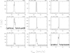 |
Fig. 14 Selected H2O maser spectra of RR Aql. The calendar date of the observation is indicated on the top left above each panel, the TJD (JD-2 440 000.5), on the top right. |
5.1 Variations of the H2O maser profile
RR Aql was first observed at Medicina in 1987 (Comoretto et al. 1990), and we monitored the star regularly between 1990 and 2011. Additional observations were made in 2015. As before 1987, the strongest maser features were always detected close to the stellar velocity (~26–31 km s−1). In Fig. 14 representative maser spectra from our observations taken between 1990 and 2011 are shown, while the complete set of 89 spectra is displayed in Fig. C.2. An overview on the general behaviour of the maser variations is shown in the FVt-plot (Fig. 15, left panel). Because of only occasional observations between June 1995 and December 2001, the plot is split into two panels omitting 3.5 yr between July 1997 and November 2000. As in U Her, the profile in general is varying with stellar pulsation in brightness and velocity range and is dominated by three features (cf. upper envelope spectrum Fig. 16), which change their relative strengths over time. The central emission at ~29 km s−1 (spectral component C hereafter) is always present (cf. lower envelope spectrum Fig. 17) and is the dominating emission for most of the time. A second feature at <28 km s−1 (spectral component A; Fig. 15, right panel) is blueshifted and is the strongest only occasionally: In 1991– 1992 (TJD ~ 8200–8900) and September/October 2001 (TJD ~ 12 200). The third feature at >30 km s−1 (spectral component E) is redshifted and was always weaker than the other two. This feature reached a ~50 Jy level between September 2004 and February 2005 (TJD ~ 13 200–13 500), while it rarely surpassed 10 Jy for the rest of the time. It was often not detected during the faint phase of the optical brightness variations.
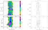 |
Fig. 15 Maser profiles as a function of time for RR Aql. Left: FVt-plot for RR Aql (cf. Fig. 2 for details). First spectrum: 17 February 1990; JD = 2 447 939.5, TJD = 7939. and last spectrum: 25 June 1997 (lower panel). First spectrum: 20 December 2000 and last spectrum: 20 March 2011 (upper panel). Right: spectral components identified by the component fit of the single-dish spectra as listed in Table B.1. |
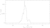 |
Fig. 16 Upper envelope spectrum for RR Aql; 1987–2015. |
5.2 H2O maser velocity range
As velocity boundaries of the maximum H2O maser velocity range ΔVloS of RR Aql we determined Vb = 23.2 and Vr = 31.9 km s−1 (Table 1) from the detection rate histogram (Fig. 18). The blue boundary is not well defined as the emission between Vlos = 21.5 and 24 km s−1 is generally weak (seen only marginally in Fig. 16) and surpasses flux densities >l Jy usually only at velocities Vlos > 25 km s−1 as evident from the FVt-plot (Fig. 15).
As in U Her, the FVt-plot shows that the width of the observed velocity range is varying. The width is smaller during the faint part of the stellar variability cycle, when the weaker outer parts of the maser profile fall below the threshold of the FVt-plot (~ 1 Jy). Close to the maxima of the stellar light curve, maser emission is seen over the maximum velocity range, except for the emission at <25 km s−1, which was detectable only in 1991 (TJD ~ 8600). In 2009, toward the end of the monitoring program, spectral component E at 30.5 km s−1 was becoming weaker and indeed was then only marginally detected in some of our 2010 and 2015 observations close to the optical maxima (cf. Appendix B).
The maximum H2O maser velocity range ΔVlos between 23.2 and 31.9 km s−1 is asymmetric with respect to V* = 28.5 with emission from the front side of the shell reaching higher outflow velocities (Vout ~ 4.5–6.5 km s−1) compared to the back side (Vout ~ 3 km s−1). It is quite likely that this velocity range is only representative for the brightest maser features. Johnston et al. (1985) detected in March 1982 with their sensitive VLA observations (rms ~ 0.35 Jy) emission between 19.7 and 36.9 km s−1. Such a large H2O maser emission range was never confirmed later on, but it may indicate that in RR Aql H2O maser emission can be present over almost the full velocity range V* − Vexp < Vlos < V* + Vexp (19.5–37.5 km s−1; Table 1) determined by the stellar wind, but is detectable only under exceptional circumstances.
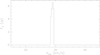 |
Fig. 17 Lower envelope spectrum for RR Aql; 1987–2015. |
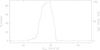 |
Fig. 18 Detection rate histogram for RR Aql; 1987–2015. |
5.3 H2O maser line profile analysis
To probe velocity variations of the features we made a similar profile analysis as for U Her (Sect. 4.1.7) by fitting Gaussian profiles to the spectra. The assignment of the features to the spectral components is discussed in Appendix B. We found five features labelled as maser spectral components A–E, which could be isolated by the fitting procedure. These components identified in individual spectra are graphically displayed in Fig. 15 (right panel), where a direct comparison with the FVt-plot is possible. The corresponding flux densities and velocities are listed in Table B.1. Components A, C and E are the three dominant features in the maser profile, while components B and D could be isolated by the Gaussian fit only for some time lasting one to six years.
Three to five spectral components are sufficient to describe the H2O maser profile in the velocity range 26 < Vlos < 32. While in this range weaker maser components could not be identified, their presence is however likely, because such weaker maser emission is seen at velocities 23 ∽− 27 km s−1 (see Appendix B), although we failed to identify individual components. In contrast, there is no evidence in our spectra for emission at velocities larger than Vlos > 32 km s−1, which leads to the observed asymmetry of ΔVlos with respect to the stellar velocity.
In RR Aqľs H2O maser shell, the components A–E represent the regions with the strongest emission only (at least over some time). Due to strong blending in velocity space they overlap in the maser profile and inhibit the identification of a spectral component, if the brightness contrast with respect to stronger neighbouring components becomes too large. We consider therefore the absence of spectral component B as a distinguishable feature in the maser profiles over more than ~ 15 yr (1995–2011, cf. Appendix B) not as evidence for extinction, but merely as inability to identify the component because of its relative weakness and blending with components A and C. In 2015 the dominant feature had a velocity Vlos ≈ 28.5, which is in between the velocities seen for components B and C before, and which we assigned tentatively to component B. Also, the identification of component D over only 1.5 yr (Fig. 15, right panel) is mostly due to blending at the other times.
Blending affects also the determination of the velocities of the spectral components. As is evident from Fig. 15 (right panel) the components showed non-systematic variations in peak velocity within ~l km s−1 over time. These variations are likely caused by blending of several maser components with velocity differences smaller than the typical line widths. This is corroborated by our experience that the profiles of the spectral components occasionally split into two or even three peaks. It is also expected from interferometric maps of RR Aqľs H2O maser shell, which showed for example in 1988 about two dozen maser spots separated in velocity by 0.3 km s−1 only (Bowers & Johnston 1994).
As in U Her, a remarkable property of the H2O maser profile of RR Aql is the apparent longevity of the spectral components in particular A and C in RR Aql, which showed also the strongest emission over almost the full monitoring period of ~22 yr. No systematic velocity shifts are recognisable, leading to the conclusion that the emission regions in RR Aql have properties as those of U Her, in particular short lifetimes of at most a few years for individual maser clouds.
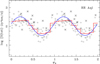 |
Fig. 19 RR Aql H2O maser light curve. See Fig. 6 for details. 5 (tot) was determined in the velocity range 22 < Vlos < 34 km s−1. The sine curve (blue) was obtained by a fit to the 1990–2011 radio measurements with a period Popt = 400 days and is delayed by ϕlag = 0.21, i.e. by 84 days with respect to the optical light curve. |
5.4 H2O maser light curve
Figure 19 shows the maser light curve of RR Aql using observations between 1990 and 2011, relative to the phase φs of the optical light curve. This radio light curve, based on integrated flux densities S (tot), and its relation to the optical light curve was analysed as for U Her. S (tot) was determined over the velocity range 22 < Vlos < 34 km s−1. The general pattern as seen in the corresponding light curve of U Her (Fig. 6) is present here as well. The selection effect discussed in Sect. 4.1.5, also in Fig. 19 leads to on average higher integrated flux densities S (tot) of the Effelsberg observations compared to those of Medicina. While the maser emission varies on average following the optical light curve, the emission for a particular phase shows a large scatter.
A fit of a sine wave to the radio data was made separately for the time ranges 1990–1997 and 2000–2011. We found little evidence for periodic variability in the first time range and a single dominating period of 405 ± 10 days in the second time range. A fit to the complete data set 1990–2011 yielded a period of 400 ± 5 days (Table 1), which coincides with the mean optical period in the time range 1987–2015. Our optical model light curve for RR Aql has a period Popt = 400 ± 2 days and a reference epoch for maxima TJDmax = 6487 ± 5 days (Table 1); these numbers were determined as described in Sect. 4.1.4 for U Her. The lag ϕlag = 0.21 (Table 1) of the radio light curve is similar to the one of U Her (ϕlag = 0.16) and other Mira variables of the sample that we monitored (Brand et al., in prep.).
The significant brightness scatter seen in Fig. 19 is caused by non-periodic brightness variations, which are caused by relative strength variations of the different spectral components. An overview of the integrated flux density light curve with (truncated) Julian Date is shown in Fig. 20. The curve is dominated by the periodic variations of the maser integrated flux density, but superposed is an apparently bright period (8500 < TJD < 9500; ~ 1991−∽1995) and a relatively faint period after TJD ≈ 13 500 (2005–2011). A zoom-in on the light curve for 1990–1997 is shown in Fig. 21, where we show also the emission contributions S (blue) and S (red) of the blueshifted Vlos < 28.5 km s−1 and red-shifted >28.5 velocity range respectively, where V* = 28.5 km s−1 is the adopted stellar radial velocity. Almost all the extra emission seen in this period is coming from the blueshifted velocity range and is caused by the extraordinary strength of spectral component B in this epoch. Except for a few months in 2001 (TJD ≈ 12 200), where spectral component A was strong, the emission in the blueshifted velocity range remained modest after 2000, and the H2O maser light curve was reflecting mostly the variations of spectral component C. After 2005 the light curve was following the overall decline of component C. Such long-term trends can be followed on timescales of several years longer than the stellar period (1.1 yr).
Another way to show the role of the secular variations of the individual spectral components is shown in Fig. 22, where the ratio R = S (blue)/S (red) is given as function of (truncated) Julian date. The prevalence of S (blue) is obvious in 8000 < TJD < 9000, but also the phase of dominance of the emission S (red) in the redshifted velocity range is evident around in 13 000 < TJD < 14 500. Typical spectra in these phases are shown in Fig. 14: On 25 October 1991 (TJD = 8554) showing spectral components A and B dominating and in 2005/2007 (TJD = 13 359/14 116) showing spectral component C dominating.
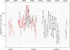 |
Fig. 20 RR Aql H2O maser light curves of the integrated flux densities 5 (tot) from Pushchino 1980–1997 (red) and Medicina/Effelsberg 1987– 2015. Vertical dotted lines are the (modelled) optical maxima with P = 400 days. |
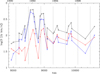 |
Fig. 21 RR Aql Medicina/Effelsberg H2O maser light curves 1990 - 1997 of RR Aql showing the emission in the Vlos < 28.5 and >28.5 km s−1 part of the maser velocity range in blue and red colour respectively. The sum of both (in black) is the integrated flux densities 5 (tot) as shown in Fig. 20. Vertical dotted lines as in Fig. 20. |
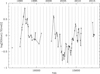 |
Fig. 22 Ratio R = 5 (blue)/5 (red) of the H2O maser emission of RR Aql of the Vlos < 28.5 (5 (blue)) and >28.5 km s−1 (5 (red)) part of the maser velocity range in 1987–2015 of RR Aql. The vertical dotted lines are optical maxima as in Fig. 20. |
5.5 Comparison with the Pushchino and VERA-lriki monitoring programs
In constrast to U Her, RR Aql was monitored also by other groups, allowing verification of our results. The Pushchino H2O maser monitoring program (B98) of RR Aql between 1980 and 1997 overlapped with ours in 1990–1997. Figure 20 shows the light curve of integrated flux density of the H2O maser between 1980 and 2011 combining observations of both monitoring programs. Both light curves are consistent with each other, although smaller brightness differences occur. This is caused likely by short-term brightness variations of the maser, leading to small brightness differences for observations made within several days.
The Pushchino light curve shows the regular brightness variations connected to the stellar pulsations clearly. In agreement with our average phase lag ϕlag = 0.21, B98 could show that these variations are following the optical variations of the star with a delay of 10–30% of the length of the period. The Pushchino light curve also confirms the long-term change of the average brightness level in ~1991 – ~1995 (8500 < TJD < 9500), caused by spectral component B at 28 km s−1 reaching flux density levels >400 Jy.
Parallel to our monitoring program, observations were made also within the VERA-Iriki monitoring program by Shintani et al. (2008) between 2003 and 2006. Within the 3.3 yr of the VERA-Iriki observations no long-term trends could be studied. In accordance with our observations, spectral components A, C and E were found to be dominant also in their observations.
The strongest features reported by single epoch observations overlapping with our monitoring program before 2000 were in April/May 1991 at 27.9 km s−1 (our spectral component B) (Takaba et al. 1994) and in October/November 1991 at 26.9 km s−1 (our spectral component A) (Takaba et al. 2001). These velocities are in agreement with our strong components seen at these times. In October 1991 spectral components A and B were competing in brightness, and in our spectrum of 25 October 1991 component B was actually 40% brighter than component A. After 2000 only one single epoch observation was made. In accordance with our observations that component E became very weak after May 2009 (see Appendix B.3), Kim et al. (2010) showed from their June 2009 observation that the component was indeed getting fainter.
6 H2O maser properties in Mira variable stars
6.1 H2O maser and optical variability: Phase lags
The prevailing pattern of the H2O maser brightness variations in U Her and RR Aql are the periodic variations, which respond to the brightness variations of the central stars. Their maser variations lag behind the optical variations by ϕlag = 0.16 and 0.21, respectively. Similar lags were also found for two other Mira variables o Cet and R Cas, monitored by us, and discussed in a separate paper (Brand et al., in prep.). The retarded maser variations are a well known pattern for Mira variables (Schwartz et al. 1974; Little Marenin & Benson 1991; Rudnitskii & Pashchenko 2005 and references therein) and red supergiants (Pashchenko & Rudnitskii 1999; Lekht et al. 2005), where the stellar brightness variations have a large amplitude. This differs from the pattern seen in semiregular variables of type SRb, such as RX Boo and SV Peg (Paper I), R Crt and RT Vir (Lekht et al. 1999; Paper II), which do not show large-amplitude periodic variations. The delayed response of maser emission to stellar brightness variations is a general characteristic, and this behaviour is well documented also for SiO masers (Pardo et al. 2004) and OH masers (Fillit et al. 1977; Etoka & Le Squeren 2000).
The lags have often been interpreted as the result of the travel time of propagating shock waves through the H2O maser zone (Lekht et al. 2001; Pashchenko & Rudnitskii 2004). Shintani et al. (2008) observed periodic velocity variations of maser features in several stars as a general pattern, which they consider as confirmation for the passage of shocks, which first accelerate and later decelerate affected maser clouds. However, lags are also seen in the infrared (Lockwood & Wing 1971; Smith et al. 2002, 2006; Ita et al. 2021). Infrared, SiO and H2O maser emissions all peak in brightness in the CSE at different distances, and so the lags, having a uniform magnitude, cannot be due to travel time effects. Guided by the findings of Shintani et al. (2008) of periodic velocity shifts in a large number of H2O maser features of several stars, we searched for patterns in the apparent velocity variations of the major spectral components G′ and G″ of U Her and component C of RR Aql. We found no regularity in the peak velocity changes over time, and conclude that the variations confined to <0.5 km s−1 are due to the influence of weaker maser features with similar velocities on the peak velocities derived from the Gaussian fits.
For the Mira variable BX Cam, periodic velocity variations were not found either, but systematic velocity drifts <1.3 km s−1 over timescales of 2–3 yr were detected in many maser spectral features, with the blue/redshifted components decreasing/increasing in Vlos, which is consistent with expansion (Xu et al. 2022).
If the shock waves propagate radially outwards, their influence on the velocities Vlos of the stronger spectral components of U Her (components G′, G″) and RR Aql (component C) furthermore is diminished due the small inclination angles of the outflow directions with respect to the plane of the sky. We were not able to find any evidence for the presence of shock waves in the H2O maser shells of the two Mira variables. We therefore consider the more likely explanation of the lags of the maser brightness variations relative to the optical to be the presence of strong titanium oxide (TiO) absorptions in the visual band at stellar maximum, as was invoked to explain the lags in the infrared by Smith et al. (2006). They find that the TiO absorption truncates the rise in the optical light before the maximum in the near-infrared is achieved. Therefore, the phase-lags are not relevant for the understanding of the conditions in the stellar wind, which allow the emergence of H2O maser emission. The phases of the H2O maser light curves are therefore probably better indicators of the phases of the stellar bolometric variations than those of the much more frequently available optical light curves.
6.2 Short- and long-term maser variability
We found compelling evidence that the H2O maser brightness variations in the SRVs R Crt and RT Vir are a superposition of two types of variations with different timescales. There are short-term fluctuations on timescales ≲1.5 yr, and long-term variations on timescales of decades (Paper II). In the case of the Mira variables U Her and RR Aql these two types of variations are also present and lead to significant cycle-to-cycle variations of the otherwise periodically varying maser light curves (Figs. 6 and 19).
The short-term fluctuations seen in integrated flux density are caused by random brightness variations of the individual spectral components, as has been shown for example for the 1991 −∽1995 absolute maximum of RR Aql’s light curve (Fig. 21 and Sect. 5.5). These short-term variations are probably controlled by the coming and going of individual maser clouds, as the limited lifetimes we found for the maser clouds of U Her indicate.
Very strong short-term fluctuations (‘bursts’) of individual spectral components at times can dominate the maser profile. Such bursts found in Mira and SR variables by the Pushchino monitoring programs (Lekht et al. 1999; Esipov et al. 1999; Pashchenko & Rudnitskii 2004) and observed by us for example in RX Boo (Paper I), in R Crt and RT Vir (Paper II), were not seen in the case of U Her (1990–2015, Fig. 7) or RR Aql (1980– 2015, Fig. 20) (although as mentioned in Sect. 4.1.6 the strong emission during the ‘1991/1992 peculiar phase’ of U Her might have been a burst). We assume that bursts are common but that their frequency of occurrence is not large, so that the absence of bursts in the latter two cases could be due to still insufficient time coverage of the maser light curves.
Long-term maser brightness variations lasting many pulsation cycles are evident for the two Mira variables, if the H2O maser light curves are displayed as function of time, either integrated over the full profiles or in selected velocity ranges. There is overall dimming and brightening of the different spectral components unrelated to each other, which determine the overall brighteness level but also their relative contributions to it. This basically reflects the change of the excitation conditions in the different parts of the H2O maser shell, which occur on timescales which are closer to the crossing time (8.5 yr in the case of U Her) of material through their H2O maser shell than to the period of stellar pulsations.
6.3 Lifetimes of H2O maser clouds
It was not possible to obtain constraints on the lifetimes of individual maser clouds in the winds of the two Mira variables based on the emergence and disappearance of individual maser features in the single-dish spectra. This is due to the wealth of components, which overlap in velocity space. The relative brightness fluctuations lead to small velocity shifts for the spectral components, and so individual maser components may be detectable individually in the spectral profiles only during short times when they are strong.
The smaller number of spectral components identified in the H2O maser profile of RR Aql compared to U Her is likely also a consequence of blending in velocity space. The final expansion velocity of RR Aql’s wind is about 65% of that of the wind of U Her (Table 1), and so the acceleration in the H2O maser shell is smaller. Given the same spectral resolution, separating the spectral components is then more difficult, assuming that the number of maser clouds and the line width distribution of the maser features are comparable in both stars. The spatially resolved maps are the only means to break the degeneracy present in velocity space. We identified nearly 30 different spatial components in the 1990–1992 VLA maps of U Her compared to fewer than 10 spectral components in the single-dish spectra detected during this period. Based on the VLA map from Bowers & Johnston (1994) a similar discrepancy in the numbers of spatial and spectral components is present also for RR Aql.
The lifetimes can be constrained by the apparent absence of acceleration of the spectral components (cf. Sect. 4.5.1). In both stars they showed constant Vlos over the monitoring period independently from their location in the maser profile. If the emission clouds participate in the stellar outflow, their outflow velocities will increase with time and so, therefore, will their absolute projected velocities, modified by the inclination of the outflow direction with respect to the plane of the sky. The expected velocity drifts are not seen (see the FVt-plots Figs. 2 and 15). This observation can be reconciled, if the emission clouds are themselves short-lived and new clouds regularly emerge in a longer-living (stationary?) larger region within the shell, as we have discussed for UHer (cf. Sect. 4.5.2). The clouds would then be created with similar Vlos, and following each other would make up a spectral component with constant velocity. The presence of such regions is also suggested by the mapping observations of BX Cam in 2012–2014 by Matsuno et al. (2020) and in 2018–2021 by Xu et al. (2022), where the emission sites were found in the same parts of the maser shell, despite the stellar wind material in the shell having been exchanged completely between the epochs, given the crossing time of 7.6 yr reported by the latter authors.
As the clouds follow the stellar wind with increasing outflow velocities, the spectral components in principle cannot have a strictly constant velocity. Our velocity outflow model (Eq. (2)) for UHer predicts an acceleration of 0.5 km s−1yr−1 in the centre of the shell. Adopting a typical lifetime of 2 yr (Bains et al. 2003), a maser cloud will therefore have changed its outflow velocity by 1.0 km s−1 and its line-of-sight velocity by ≤1 km s−1. Velocity drifts of this size are in agreement with the systematic increase/decrease of Vlos by up to ~0.4 km s−1yr−1 observed for the H2O maser spectral features in BX Cam by Xu et al. (2022). According to our model, the cloud also will have moved radially by 3–4 AU during its 2 yr lifetime. For U Her, Richards et al. (2012) found an increase of the Vlos with distance from the star and derived a velocity gradient in the plane of the sky of 0.31 ± 0.28 km s−1 AU−1. A gradient of 0.31 km s−1 AU−1 translates to a drift in outflow velocity by 0.9–1.2 km s−1 for a movement over 3–4 AU, which is compatible with our estimate of its change in outflow velocity derived above from the model. We conclude that the drifts in Vlos of the spectral components, which are expected to be ≤ 1 km s−1 over two years are masked in our single-dish data, because the size of the drifts is of the order of the uncertainties in our velocity determinations due to blending with neighbouring features. Components with aspect angles >30º would have drifts in Vlos, which surpass our limit of 0.5 km s−1. Of the spatial components plotted in Fig. 13 that have aspect angles θ > 30º, only B and C are strong enough to be seen contiguously for over more than a year. These components are seen between 1990 and 1996 (see Fig. 2). They would be good candidates for the detection of drifts (for B one expects 0.9 km s−1 in two years), but none are seen. They play a prominent role in the ‘1991/1992 peculiar phase’ and their behaviour points to lifetimes <2 yr, maybe even months (see discussion in Appendix A). The apparent constant velocity of the spectral components as shown in the U Her’s FVt-plot (Fig. 2) is therefore due to the superposition of clouds created with almost equal velocities and replacing each other every few years. The clouds should have systematic velocity drifts over typical maser cloud lifetimes, but these are not detectable in our single-dish spectra.
6.4 Long-living regions
The long-term maser brightness variations and the observation that the clouds responsible for the strongest spectral components in U Her are found in the same region of the maser shell over at least 6.5 yr (almost 6 stellar pulsation cycles), indicate the presence of inhomogeneities in the otherwise (assumed) spherical stellar wind of Mira variables. One indicator for such inhomo-geneities could be parts of the shell, where the conditions are more favourable for exciting the H2O molecules (‘long-living regions’) than in others. While individual (maser) clouds would be clumps of material with enhanced density moving with the stellar wind, such regions remain stationary in location, at least as long as the wind is not disturbed at these locations. The individual clouds then light up, while they pass through the regions. The existence of such regions would then naturally explain, why maser spectral components like component K in U Her (see Sect. 4.5) regularly reappear over about 15 yr at almost the same Vlos, although different short-living maser clouds must have contributed.
Also, in the SRVs RX Boo, RT Vir, and R Crt, we previously found evidence for the existence of long-living regions within the H2O maser shell, in which preferred conditions for exciting the H2O molecules exist. In RX Boo they manifested themselves as spatial asymmetries of the H2O maser emission persistent for at least 11 yr (Paper I). For RT Vir and R Crt, the decade long variations of the H2O maser brightness in particular velocity ranges, was attributed to such regions having possibly higher-than-average densities and being present in the H2O maser shells for about two decades (Paper II). Based on 3D models of Freytag & Höfner (2023) (and preceding papers) we argued that such regions could be the remnants of large convective cells, which left the stars as part of the stellar winds. Having reached the H2O maser shell they may have been inflated to sizes comparable to the width of the maser shells. They may provide the shell sectors with improved maser excitation conditions, in which clouds passing through are preferentially excited. Observationally it would lead to an asymmetric spatial maser distribution within an otherwise spherical symmetric H2O maser shell. If the presence of (sub)stellar companions plays a major role in shaping the stellar winds (Decin et al. 2020; Gottlieb et al. 2022), their influence on the velocity field may be another factor to create long-living regions with improved excitation conditions. These regions could be in parts of the shell relatively far from companions, where the stellar wind is less disturbed. Lifetimes of the long-living regions would probably be of the order of the crossing time of material through the shell or of the orbital periods of the companions.
While the spherical H2O maser shell is a persistent feature with some variations of its boundaries, the maser clouds are a transient phenomenon with a lifetime of a few years. The regions, in which favourable excitation conditions for H2O maser emission occur, are intermediate in the sense that they are part of the H2O maser shell, but not lasting. They have long but limited lifetimes, because of the inhomogeneity of the stellar wind. Over time, such regions where maser clouds pass through are created at different locations within the shell.
H2O maser luminosities, stellar luminosities, and mass-loss rates of the semiregular variable stars from Paper I and II and the Mira variables U Her and RR Aql.
6.5 H2O maser luminosities
In Table 5, we give luminosity information on U Her and RR Aql, as well as those of the four SRVs treated in Paper I and II. For the details of how the luminosities were derived, we refer to Paper II. In Col. 4, we give  , the potential maximum H2O maser luminosity derived from the upper envelope, which represents the maximum output which the source could produce if all the velocity components we observe were to emit at their maximum level, at the same time and equally in all directions. The table also lists characteristic levels (high, mean, and low) of maser brightnesses, as given by integrated flux densities S (tot) in Jy km s−1 (Cols. 5,7,9) and corresponding maser luminosities Lp in photons per second (Cols. 6,8,10). The brightness of the mean level is the median of all integrated flux density measurements while the high and low level are represented by the median of the seven highest and lowest integrated flux density measurements, respectively.
Table 5 shows that the mean maser luminosities of U Her and RR Aql (as well as  ) are in the range of luminosities shown by the SRVs. The ratio between the high and low level of the two Mira variables is 15–20, which is slightly higher than for the four SRVs with ratios >6–16 (>35–45 between
  and the low levels of Lp compared to >25–55 of the SRVs).
As in Paper II, we compared the H2O maser photon luminosities with the bolometric luminosities and mass-loss rates of the stars. The bolometric luminosities Lbol (Col. 11) were determined from bolometric fluxes, as described in Jiménez-Esteban & Engels (2015), and the distances listed in Table 5. The mass-loss rates Ṁ (Col. 12) were taken from Loup et al. (1993) (U Her) and Danilovich et al. (2015) (RR Aql) scaled to the distances used here. All mass-loss rates come from measurements of the CO molecular line and are estimated to have an error of a factor of 3 (=0.5 dex) prior to the uncertainties introduced by the distances. We note however, that due to a general underestimate of the terminal stellar wind velocities in the past, these mass-loss rates could be systematically underestimated (Gottlieb et al. 2022). The results are listed together with those of the SRVs (see Paper II) in the last two columns of Table 5.
We find that the two Mira variables have stellar luminosities and mass-loss rates within the range shown by the SRVs. Not surprisingly also the H2O maser photon luminosities fit well within the range of those of the SRVs. The stars selected by us for H2O maser monitoring all showed apparently bright masers since their discovery. Except for SV Peg, all of them appear among the 10% brightest galactic H2O masers in late-type stars known by the year 2000 on the sky north of δ > −30° (Valdettaro et al. 2001). Besides a few Red Supergiants this list of late-type stars is composed of optically bright Mira and SR variables. It is therefore obvious that the stars from our monitoring program represent only the upper end of the photon luminosity distribution of H2O masers of Mira and SR variables in the solar neighbourhood.
6.6 Constraints on the CSE standard model
The analysis and discussion of the H2O maser properties of U Her and RR Aql are based on the standard model, which assumes the presence of a spherical H2O maser shell within a circumstellar envelope continuously fed by a homogeneous spherically outflowing stellar wind with smoothly increasing velocities. The stellar pulsations naturally lead to maser brightness variations and connected with this to variations of the velocity range over which emission is detected above the sensitivity limit. The boundaries of the maser shell are, strictly speaking, boundaries for luminous maser sites, and may change over time due to evolution of the excitation conditions and changes in beaming directions. The time coverage of the maser observations since their discovery is still too short to provide information on the origins of the long-term variations, but they indicate that there are regions of improved excitation conditions within the maser shell – as discussed in Sect. 6.4 – and therefore inhomogeneities in the spherical outflow.
The filling factor of detectable maser clouds within the maser shell is rather small (Richards et al. 2012) and so asymmetries seen in maser maps can be due either to accidentally emerging illumination variations, or is another indication that the underlying stellar wind itself is inhomogeneous. 3D models of the formation of dust-driven winds in AGB stars by Freytag & Höfner (2023), indicate that the stellar wind starts clumpy above the photosphere. It is not clear how much of the clumpiness is still present at the location of the H2O maser shell (10–30 AU from the star for SRV and Mira variables), but the related velocity variations of the wind due to shock waves generated close to the photosphere may have become negligible at these distances (Bladh et al. 2019). Smoothly increasing outflow velocities described by a velocity law with continuous acceleration and approaching a constant outflow at large distances, as for example expressed by Eq. (2), may therefore still be applicable.
However, new observations of several molecular species and transitions in the CSEs of several AGB stars and RSGs challenge the validity of such a law (Gottlieb et al. 2022). While these authors observe an overall increase of outflow velocities with radial distances, the scatter is not compatible with a smooth velocity law. The scatter is ascribed to the presence of a (sub)stellar companion which disturbs the velocity field. In addition, they find that the final expansion velocities are up to a factor of two higher than previously adopted. For U Her this is Vexp = 19.7 km s−1 compared to 13.1 km s−1 as adopted by us (Table 1). RR Aql was not observed. Their outflow velocity law for U Her is V(r) = V0 + (Vexp − V0) • (1 − r0/r)β, where r0 = 2.6 R*, V0 ~ 4.4 km s−1 and β = 2.00 ± 0.54. Parameter r0 is the dust condensation radius, where the wind starts, and V0 is the velocity at this radius. This law is considered an approximation and is given for distances in the CSE between ~2.6 and 500 R* (~4−700 AU).
Adopting this law in our model of the H2O maser shell (Sect. 4.3), the larger final expansion velocity leads to an increase of the acceleration in particular in the inner shell, where the H2O masers are located. For example at radial distance r =18 AU the increase is from 0.5 to 1 km s−1yr−1. Correspondingly the crossing time and the lifetimes derived for individual maser clouds are decreased by a factor of~1.8.
As long as acceleration is present in the H2O maser shell, the absence of velocity drifts of the H2O maser spectral components constrains the lifetimes of the maser emitting clouds. A lifetime larger than the monitoring period of 22 yr, would require a rather small acceleration a < 0.023/sinθ km s−1yr−1 to avoid shifts in Vlos |ΔVlos| > 0.5 km s−1 (see Sect. 4.5.1). This would need almost a suspension of the acceleration within the H2O maser shell (i.e. a step-wise increase of the velocity curve as discussed by Decin et al. (2015) in the case of the carbon star IRC+10216) or an approach to the final expansion velocity already at the inner maser shell radius. We adopted the latter explanation for the SRV RT Vir, where we observed a maser feature showing a constant velocity within <0.06 km s−1 over 7.5 yr. We suggested the maser-emitting cloud to move in the outer part of the shell, where the final expansion velocity could have been reached already. The alternative, maser clouds with short lifetimes created again and again, was considered as less likely because of the very small velocity scatter (Paper II).
So far, a step-wise increase of the velocity curve has not been considered to explain the observed velocities in the H2O maser shell. The model presented in Sect. 4.3 for U Her is strictly constrained only by the outflow velocity Vout = 9.6 km s−1 at a radial distance of 23.9 AU. Forcing the adopted velocity law to start at the photosphere (r0 = 1.4 AU, V0 = 0 km s−1) is a rather coarse assumption given that in U Her’s CSE, H2O line emission from the (0,2,0) 652 − 743 transition at 268 GHz line was detected over a velocity range −24.2 to −4.5 km s−1 by Baudry et al. (2023) within a projected distance of ~3.2 AU from the centre of the star. This implies gas motions with outflow and infall of up to 10 km s−1 in the inner shell, and a smooth velocity law may not be applicable within several stellar radii from the star.
In principle, the outflow velocity could reach Vout = 9.6 km s−1 at the inner maser shell boundary, stay constant up to the outer maser shell boundary, and increase further beyond. In the case of a step-wise increase of the velocity curve, a section with constant velocity of 9.6 km s−1 will have improved velocity coherence, and naturally delineate the shell, where H2O maser emission preferentially occurs. The boundaries at ~5 and ~30 AU would be determined by the loss of velocity coherence outside the section with constant outflow velocity. However, marginal acceleration would favour radial amplification paths and one would expect double-peaked maser profiles strongest close to ± Vout (in our case ±9.6 km s−1) as seen for 1612 MHz OH masers, which are excited at much larger distances from the star, where the outflow velocity also in the standard model is almost constant. This is however not observed, as H2O maser profiles of SR- and Mira variables generally peak close to the stellar velocity (Takaba et al. 1994), meaning that tangential maser amplifications paths are preferred to radial ones. Richards et al. (2012) also argue against an absence of acceleration within the H2O maser shell, as they found that in the shells of all observed AGB and RSG stars the outflow velocity increases by a factor of two. Following the numerous indications that the velocity field of the stellar winds is likely disturbed over a great part of the CSE, we therefore consider an almost constant velocity over several AU delineating the H2O maser shell unlikely.
7 Conclusions
We analysed the properties of the H2O maser emission of two Mira variables U Her and RR Aql, which both show maser emission spread in velocity over several km s−1, with usually bright individual features (>100 Jy). Their masers are among the strongest H2O masers seen in late-type stars on the sky.
The variability of the maser emission is dominated by regular brightness variations synchronised with the stellar pulsation. As generally observed in Mira variables, the maser brightness variations are delayed relative to the optical variations; in the case of U Her and RR Aql, these delays are two and nearly three months, respectively. We attribute the cause of this phase-lag to the influence of absorption by molecular bands on the optical light curve. Superposed on the regular variations are brightness fluctuations on shorter timescales, which are due to secular variations of individual spectral components. Also, on longer timescales, variations are seen of the average brightness level in both stars.
The brightness levels in the blueshifted and redshifted velocity ranges show (on these timescales) variations that are independent from each other. This indicates that the stellar wind is inhomoge-neous, which leads to varying excitation conditions in the front and rear cap of the H2O maser shell. This change in excitation conditions can lead to a completely different spectral profile, where in the case of U Her the usually dominating profile peak at −15 km s−1 was exceeded for 1.5 yr by peaks at < −18 km s−1 (‘1991/1992 peculiar phase’). Apart from that, the H2O maser variability patterns of U Her and RR Aql are remarkably similar.
Based on our VLA observations 1990–1992, we find that the H2O masers of U Her were located in a spherical shell with a size of 11–25 AU. Additional weak maser emission was found inside and outside these boundaries. Comparing this result with interferometric observations from the literature obtained at other epochs shows some variations of the size, but in general the strongest emission comes from radial distances of ~15–20 AU. With a radius of ~21 AU reported for RR Aql’s H2O maser shell, also the shell dimensions corroborate the similarity of the H2O maser properties between U Her and RR Aql.
The absence of velocity drifts is strong evidence in favour of short lifetimes of maser clouds (about <4 yr). The location of the main emission features of U Her in the same part of the H2O maser shell over at least 6.5 yr and the regular reappearance of emission at the same velocity (see component K in U Her) support the idea of there being long-living regions or sections of the maser shell with favourable excitation conditions, which last over timescales longer than the stellar period and the lifetime of individual maser clouds.
The H2O maser luminosities of the two Mira variables are within the range of luminosities derived in Paper I and II for SRVs. These objects have variation properties that are very similar to those of SRVs, except for their periodic variations as a consequence of the stellar pulsation (via pumping variations).
Variability is present on several timescales, meaning that the conclusions drawn from our monitoring program - lasting more than two decades – are strictly only valid for the scales covered. For U Her, the length of the monitoring program is about twice the time needed for the stellar wind to cross the H2O maser shell. Variations in the mass-loss rates on longer timescales (hundreds to thousands of years) may lead to a loss of U Her’s and RR Aql’s prominent status among the strongest circumstellar H2O masers observed from Earth; they may even join the much larger group of Mira variables that are currently not detected with H2O masers, while in other Mira variables H2O maser emission may brighten and/or be beamed into our line of sight.
As the validity of a smooth acceleration of the stellar wind was recently brought into question, the use of H2O masers to trace the velocity field of the inner wind region of AGB stars (r ≲ 20 R*) should gain importance.
Acknowledgements
The Medicina 32 m data presented here are part of a long-term monitoring program, which concerned both late-type stars and star-forming regions. Thanks to those who helped with the observations. We are grateful to the staff at Medicina observatory for their expert assistence and technical problem-solving. The Medicina radio telescope is funded by the Ministry of University and Research (MUR) and is operated as National Facility by the National Institute for Astrophysics (INAF). This research is partly based on observations with the 100 m telescope of the MPIfR (Max-Planck-Institut für Radioastronomie) at Effelsberg, and the VLA (Very Large Array). The VLA is operated by the National Radio Astronomy Observatory, which is a facility of the National Science Foundation operated under cooperative agreement by Associated Universities, Inc. This research has made use of the SIMBAD database and the VizieR catalogue access tool, operated at CDS, Strasbourg, France, and of NASA’s Astrophysics Data System. For data reduction and the preparation of figures GILDAS software available at www.iram.fr/IRAMFR/GILDAS was used. We acknowledge with gratitude the variable star observations from the AAVSO International Database contributed by observers worldwide and used in this research. The spectra are available in FITS-format at the CDS;also the VLA data cubes can be downloaded from there. The tables from the appendix are available at the CDS as well.
Appendix A U Her spectral line fitting results
The maser features identified between 1987 and 2015 in the individual spectra are listed in Tables A.1 and A.2, where they were assigned to different spectral components separated through Gaussian fits. For each spectrum we give the Gregorian and Julian dates, its rms noise level in Jansky, the integrated flux densities S (tot) in Jy km s−1, the phase of the optical light curve φs, and the velocity (Vp) and peak flux density (Sp) for each component. Flux density values marked by ‘:’ and upper limits were measured with the cursor on the computer screen. Velocity values marked by ‘:’ are uncertain. φs was calculated for each observing date using the optical period and a reference epoch for the optical maxima TJDmax (i.e. φs = 0), as given in Table 1. In the following we discuss in detail the variations in flux density and velocity of the spectral components, for the main velocity ranges discussed in the main body of the paper.
Appendix A.1 The Vlos < −18 km s−1 velocity range
The most blueshifted emission observed by us in 1987 – 2015 was detected at −23.8 km s−1 in the Oct. 1991 VLA observation (spatial component A1 in Table 3). The emission was weak (≈0.4 Jy/beam) and not seen in the single-dish spectra of this epoch. Emission at velocities < −22 km s−1 was seen in the single-dish spectra only occasionally and was blended with the stronger spectral component B. The most blueshifted emission detected in Effelsberg and Medicina was seen in 1995 with a peak at −22 km s−1and extending down to −23.3 km s−1, while the star was increasing its optical brightness (0.7 < φs < 1.0). The emission was on the ≈1 Jy level. We therefore conclude that in the velocity range −24 < Vlos < −22 km s−1 (the location of a putative spectral component A) maser emission was probably present, although below our detection limits most of the time.
In addition to this low-level emission we identified three spectral components B–D at velocities Vlos < −18 km s−1. The emission in the −22 < Vlos < −20 km s−1 region (spectral component B) was seen only until 1996 and was in general about a factor of 10–100 weaker than emission at higher velocities. Only during a very brief period (the ‘1991/1992 peculiar phase’) in Oct./Nov. 1991 (TJD = 8959) component B (then at −20.6 km s−1) was the strongest of all spectral components (Fig. 1). The component was not detected in May 1991 and declined by a factor of ~ 15 until January 1992.
During the ‘1991/1992 peculiar phase’, emission at −20 < Vlos < −19 km s−1 (spectral component C) increased in intensity after May 1991 (TJD ~ 8400), reached its peak in Jan. 1992 (TJD ~ 8640) and faded to the level seen before and afterwards until March 1992 (TJD ~ 8700). A similar short dominance was seen in Sep. 1996 (TJD = 10353), when spectral velocity component D′ (Vlos = −18.8 km s−1) was the strongest feature in the profile. The brightenings seen in spectral components B, C, and D′ lasted typically 6 to 12 months.
The emission between Vlos = −19 and −18 km s−1 was dominated by spectral components D’ (strong in 3/1995 − 2/1997, TJD = 9790 − 10486) and D″, which often were difficult to separate in velocity space. Therefore, Tables A.1 and A.2 usually list only one of both components depending on the peak velocity provided by the Gaussian fit, although most probably both components where present. In February 1992 (TJD = 8682; φs = 0.97) component D″ reached the strongest flux density (> 300 Jy) ever observed between 1987 and 2015 for an individual spectral feature. Until October 1992 it decreased to a level of ~ 10 Jy and remained on that level until it disappeared after 2001.
Appendix A.2 The −18 < Vlos < −16 km s−1 velocity range
Often blended with spectral components D″ at −18.3 km s−1 and G′ at −15.5 km s−1 the emission in between was almost always detected. Peak velocities of the Gaussian fits varied between −17.5 and −16.5 km s−1, indicating that more than a single emission feature contributed. As these features in general could not be decomposed, they are listed together in Table A.1 as spectral component E. In the interferometric maps 1990 – 1992 we identified five spatial components E1 – E5 (Table 3).
Appendix A.3 The −16 < Vlos < −14 km s−1 velocity range
The dominant H2O maser emission stemmed almost continuously from velocities −16 < Vlos < −14 km s−1. Within this velocity range two or more spectral features contributed. Due to the variations of the relative intensities, the central velocities of the Gaussian fits drifted. Usually two features could be identified, which we designated spectral components G′ and G″ in Table A.2. In 1990, at the beginning of the systematic monitoring program two features with > 200 Jy at −15.3 (G′) and −14.7 (G″) km s−1 dominated the profile, with component G″ being the stronger one. This changed after 1991 and lasted until 2006, when again component G″ became stronger than G′. This behaviour is the cause for the apparent curvature of the ridge of the emission in the FVt-plot (Fig. 2) within the velocity interval −16 < Vlos < −14 km s−1. In 2007 – 2011 (TJD ≳ 14000) the evidence that G′ is a blend of maser lines is particularly strong, as the peak velocity varied in the interval −16.0 ≤ Vlos ≤ −14.8 and showed shifts between the extremes of this interval within four months (August - December 2007).
Appendix A.4 The Vlos > −14 km s−1 velocity range
In this fourth velocity range only weaker emission was present which was assigned to spectral components I–M in Table A.2. Spectral component I was centred most of the time at −12.9 ± 0.1 km s−1. Only between 1993 and 1995 (TJD ~ 8700 − 10200) the centre was at −13.5 ± 0.2 km s−1. After 1995 the component surpassed the detection limit only close to the maxima of the stellar lightcurve. The last four years after 2007 (TJD > 14450) it was not detectable anymore, but reappeared in 2015 during an optical maximum (Fig. C.1).
In the period 1995 − 2010 (9700 < TJD < 11700) emission was detected at ~ −11.0 km s−1 (component K), often at phases when also component I was detected and similar in strength (Fig. 2). At velocities ~ −10 km s−1, in 1990/1991 (TJD < 8400) emission with flux densities of a few Jansky was present at −10.2 km s−1. Later in a short phase of about 6 months in 2009/2010 emission was detected at at −9.7 km s−1 (Table A.2). Due to their proximity in velocity we assigned to them a common spectral component L. Components I, K and L are responsible for the distinguished feature in the FVt-plot (Fig. 2) at ~−10 km s−1 at TJD ~ 15100 − 15300.
Also seen for only a few months (Oct. 1990 − May 1991; Table A.2) was spectral component M, the most redshifted component in the H2O maser profile. It appeared at ~−8 km s−1 with flux densities ~1 Jy and is marginally visible at TJD ~ 8300 in the FVt-plot (Fig. 2).
Maser spectral components B – E of U Her
Maser spectral components G – M of U Her
Appendix B RR Aql spectral line fitting results
The maser features identified between 1987 and 2015 in individual spectra are listed in Table B.1, where they were assigned to five different spectral components labeled A–E. The corresponding Gaussian fits were made using the original spectral resolution of the individual spectra. The meaning of the columns in Table B.1 are as in Tables A.1 and A.2. In the following we discuss the variations in flux density and velocity of the spectral components.
Appendix B.1 The Vlos < 28 km s−1 velocity range
The spectral component, which was almost always detectable in this velocity range is component A centred on Vlos = 27 km s−1. It could be identified during the entire monitoring period 1990 − 2011, except for a few months in 2005 and 2007. During these months emission was present at this velocity, but was too weak to be identified by the Gaussian fitting procedure as a separate maser feature. The same applies for 2015, when the velocity of component A was within the blue wing of the maser profile. Component A occasionally became the strongest feature in the spectral profile. If it reached high brightness levels (>150 Jy), this occurred usually around the maximum of the visual light curve 0.0 ≤ φs ≤ 0.3.
Between 1990 and the beginning of 1994 spectral component B, centred on Vlos = 28 km s−1, was the strongest component in the profiles (see the 1991 spectrum in Fig. 14). With brightness levels surpassing 400 Jy (0.2 < φs < 0.4), it reached also the highest brightness among all spectral components between 1987 and 2015. In 1994, emission at this velocity became weaker. After March 1995, blending by the neighbouring spectral components A and C became so severe that component B could not be identified unambiguously with the Gaussian fitting procedure anymore. After the observing gap 2011 – 2015 component B was the dominating spectral component again, but with a slightly higher velocity of Vlos = 28.5 km s−1.
At velocities Vlos < 27 km s−1 the emission was always a factor of ≥ 10 weaker than spectral components A or B. No convincing spectral components covering more than a few spectra could be identified with the Gaussian fitting procedure.
Appendix B.2 The 28 ≤ Vlos < 30 km s−1 velocity range
This velocity range includes the stellar radial velocity V* = 28.5 km s−1 (see Table 1). The prominent feature in this velocity range is spectral component C at Vlos = 29 km s−1. It was always present, even in 2015, when the emission at 29 km s−1 was blended with the single feature seen at Vlos = 28.5 km s−1 and which we assigned to spectral component B. Component C was the strongest feature in the years 2000–2009. In 2010 and 2011 it had a similar brightness as component A, resulting sometimes in characteristic double-peaked profiles (cf. in Fig. C.2).
For about a year in 1994/1995 we could identify a component with the Gaussian fits with a velocity of Vlos = 29.8 km s−1. This component D is blended at other times with the stronger components C and E. Although emission is always present at this velocity, a separate feature could not be identified unambiguously with the Gaussian fit procedure. Component D is therefore similar to component B. When they are significantly weaker than their neighbouring components (or maybe even absent) they could not be identified due to blending in velocity space.
Appendix B.3 The Vlos ≳ 30 km s−1 velocity range
Velocities Vlos > 30 km s−1 are represented by component E at Vlos = 30.5 km s−1. In general the emission is significantly weaker than those of spectral components A, B, and C. In only one occasion component E was found to be the strongest: In our first (isolated) spectrum taken 12.6.1987 and reported also by Comoretto et al. (1990), this feature reached a peak flux density ~ 60 Jy. The maximum brightness observed during the whole monitoring time was in December 2004 / January 2005 with a flux density ~65 Jy. This indicates that in 1987 the other components were unusually weak, rather than that component E was particularly bright. The component E emission is prominent in the FVt-plot and could be identified with the Gaussian fit procedure mostly at phases after the visual maximum, when the star was bright. After May 2009 and including 2015, the spectral component disappeared from the spectra, except between March and May 2010 and in September/October 2015 (at phase φs = 0.0 ± 0.1 in both cases), when emission < 5 Jy was observed at its velocity.
Maser spectral components of RR Aql
Appendix C all maser spectra
In this section we show all H2O maser spectra of our targets. There are more spectra here than in the FVt-plots, because in those plots (apart from having averaged spectra taken within 4 days from one another) we have tried to avoid large gaps between observations, in order not to have to interpolate over large time intervals.
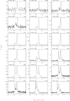 |
Fig. C.1 All H2O maser spectra of U Her. The observing date (top left) and TJD (top right) are indicated for each spectrum. |
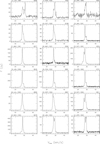 |
Fig. C.2 All H2O maser spectra of RR Aql. The observing date (top left) and TJD (top right) are indicated for each spectrum. |
References
- Bains, I., Cohen, R. J., Louridas, A., et al. 2003, MNRAS, 342, 8 [NASA ADS] [CrossRef] [Google Scholar]
- Barvainis, R., & Deguchi, S. 1989, AJ, 97, 1089 [NASA ADS] [CrossRef] [Google Scholar]
- Baudry, A., Wong, K. T., Etoka, S., et al. 2023, A&A, 674, A125 [NASA ADS] [CrossRef] [EDP Sciences] [Google Scholar]
- Berulis, I. I., Lekht, E. E., Pashchenko, M. I., & Rudnitskii, G. M. 1983, Soviet Ast., 27, 179 [Google Scholar]
- Berulis, I. I., Lekht, E. E., Munitsyn, V. A., & Rudnitskii, G. M. 1998, Astron. Rep., 42, 346 (B98) [NASA ADS] [Google Scholar]
- Bladh, S., Liljegren, S., Höfner, S., Aringer, B., & Marigo, P. 2019, A&A, 626, A100 [NASA ADS] [CrossRef] [EDP Sciences] [Google Scholar]
- Bowers, P. F., & Johnston, K. J. 1994, ApJS, 92, 189 [CrossRef] [Google Scholar]
- Bowers, P. F., Claussen, M. J., & Johnston, K. J. 1993, AJ, 105, 284 [NASA ADS] [CrossRef] [Google Scholar]
- Brand, J., Engels, D., & Winnberg, A. 2020, A&A, 644, A45 (Paper II) [NASA ADS] [CrossRef] [EDP Sciences] [Google Scholar]
- Chiavassa, A., Freytag, B., & Schultheis, M. 2018, A&A, 617, L1 [NASA ADS] [CrossRef] [EDP Sciences] [Google Scholar]
- Colomer, F., Reid, M. J., Menten, K. M., & Bujarrabal, V. 2000, A&A, 355, 979 [NASA ADS] [Google Scholar]
- Comoretto, G., Palagi, F., Cesaroni, R., et al. 1990, A&AS, 84, 179 [Google Scholar]
- Danilovich, T., Teyssier, D., Justtanont, K., et al. 2015, A&A, 581, A60 [NASA ADS] [CrossRef] [EDP Sciences] [Google Scholar]
- Decin, L., Richards, A. M. S., Neufeld, D., et al. 2015, A&A, 574, A5 [NASA ADS] [CrossRef] [EDP Sciences] [Google Scholar]
- Decin, L., Montargès, M., Richards, A. M. S., et al. 2020, Science, 369, 1497 [Google Scholar]
- Dickinson, D. F., Bechis, K. P., & Barrett, A. H. 1973, ApJ, 180, 831 [NASA ADS] [CrossRef] [Google Scholar]
- Engels, D., Schmid-Burgk, J., & Walmsley, C. M. 1988, A&A, 191, 283 [Google Scholar]
- Engels, D., Winnberg, A., Brand, J., & Walmsley, C. M. 1999, IAU Symp., 191, 373 [NASA ADS] [Google Scholar]
- Esipov, V. F., Pashchenko, M. I., Rudnitskii, G. M., & Fomin, S. V. 1999, Astron. Lett., 25, 672 [NASA ADS] [Google Scholar]
- Etoka, S., & Le Squeren, A. M. 2000, A&AS, 146, 179 [NASA ADS] [CrossRef] [EDP Sciences] [Google Scholar]
- Felli, M., Brand, J., Cesaroni, R., et al. 2007, A&A, 476, 373 [NASA ADS] [CrossRef] [EDP Sciences] [Google Scholar]
- Fillit, R., Proust, D., & Lepine, J. R. D. 1977, A&A, 58, 281 [NASA ADS] [Google Scholar]
- Freytag, B., & Höfner, S. 2023, A&A, 669, A155 [NASA ADS] [CrossRef] [EDP Sciences] [Google Scholar]
- Gaia Collaboration. 2020, VizieR Online Data Catalog: I/350 [Google Scholar]
- Gaia Collaboration (Brown, A. G. A., et al.) 2021, A&A, 649, A1 [NASA ADS] [CrossRef] [EDP Sciences] [Google Scholar]
- Gonzalez-Alfonso, E., Cernicharo, J., Alcolea, J., & Orlandi, M. A. 1998, A&A, 334, 1016 [NASA ADS] [Google Scholar]
- Gottlieb, C. A., Decin, L., Richards, A. M. S., et al. 2022, A&A, 660, A94 [CrossRef] [EDP Sciences] [Google Scholar]
- Habing, H. J. 1996, A&A Rev., 7, 97 [NASA ADS] [CrossRef] [Google Scholar]
- Höfner, S., & Olofsson, H. 2018, A&A Rev., 26, 1 [CrossRef] [Google Scholar]
- Imai, H., Sasao, T., Kameya, O., et al. 1997a, A&A, 317, L67 [NASA ADS] [Google Scholar]
- Imai, H., Shibata, K. M., Sasao, T., et al. 1997b, A&A, 319, L1 [NASA ADS] [Google Scholar]
- Imai, H., Shibata, K. M., Marvel, K. B., et al. 2003, ApJ, 590, 460 [NASA ADS] [CrossRef] [Google Scholar]
- Ita, Y., Menzies, J. W., Whitelock, P. A., et al. 2021, MNRAS, 500, 82 [Google Scholar]
- Jiménez-Esteban, F. M., & Engels, D. 2015, A&A, 579, A76 [NASA ADS] [CrossRef] [EDP Sciences] [Google Scholar]
- Johnston, K. J., Spencer, J. H., & Bowers, P. F. 1985, ApJ, 290, 660 [CrossRef] [Google Scholar]
- Kim, J., Cho, S.-H., Oh, C. S., & Byun, D.-Y. 2010, ApJS, 188, 209 [NASA ADS] [CrossRef] [Google Scholar]
- Lane, A. P., Johnston, K. J., Bowers, P. F., Spencer, J. H., & Diamond, P. J. 1987, ApJ, 323, 756 [NASA ADS] [CrossRef] [Google Scholar]
- Lekht, E. E., Mendoza-Torres, J. E., Pashchenko, M. I., & Berulis, I. I. 1999, A&A, 343, 241 [NASA ADS] [Google Scholar]
- Lekht, E. E., Mendoza-Torres, J. E., Rudnitskij, G. M., & Tolmachev, A. M. 2001, A&A, 376, 928 [NASA ADS] [CrossRef] [EDP Sciences] [Google Scholar]
- Lekht, E. E., Rudnitskij, G. M., Mendoza-Torres, J. E., & Tolmachev, A. M. 2005, A&A, 437, 127 [NASA ADS] [CrossRef] [EDP Sciences] [Google Scholar]
- Little Marenin, L. R., & Benson, P. J. 1991, ASPC Ser., 16, 73 [NASA ADS] [Google Scholar]
- Lockwood, G. W., & Wing, R. F. 1971, ApJ, 169, 63 [NASA ADS] [CrossRef] [Google Scholar]
- Loup, C., Forveille, T., Omont, A., & Paul, J. F. 1993, A&AS, 99, 291 [NASA ADS] [Google Scholar]
- Marvel, K. B. 1996, PhD thesis, New Mexico State University, USA [Google Scholar]
- Matsuno, M., Nakagawa, A., Morita, A., et al. 2020, PASJ, 72, 56 [NASA ADS] [CrossRef] [Google Scholar]
- Neufeld, D. A., Melnick, G. J., Kaufman, M. J., et al. 2017, ApJ, 843, 94 [NASA ADS] [CrossRef] [Google Scholar]
- Ochsenbein, F., Bauer, P., & Marcout, J. 2000, A&AS, 143, 23 [NASA ADS] [CrossRef] [EDP Sciences] [Google Scholar]
- Ott, M., Witzel, A., Quirrenbach, A., et al. 1994, A&A, 284, 331 [NASA ADS] [Google Scholar]
- Pardo, J. R., Alcolea, J., Bujarrabal, V., et al. 2004, A&A, 424, 145 [NASA ADS] [CrossRef] [EDP Sciences] [Google Scholar]
- Pashchenko, M. I., & Rudnitskii, G. M. 1999, Astron. Rep., 43, 311 [Google Scholar]
- Pashchenko, M. I., & Rudnitskii, G. M. 2004, Astron. Rep., 48, 380 [CrossRef] [Google Scholar]
- Press, W. H., Teukolsky, S. A., Vetterling, W. T., & Flannery, B. P. 1992, Numerical Recipes in FORTRAN (Cambridge: Cambridge University Press) [Google Scholar]
- Ragland, S., Traub, W. A., Berger, J. P., et al. 2006, ApJ, 652, 650 [NASA ADS] [CrossRef] [Google Scholar]
- Richards, A. M. S., Elitzur, M., & Yates, J. A. 2011, A&A, 525, A56 [NASA ADS] [CrossRef] [EDP Sciences] [Google Scholar]
- Richards, A. M. S., Etoka, S., Gray, M. D., et al. 2012, A&A, 546, A16 [NASA ADS] [CrossRef] [EDP Sciences] [Google Scholar]
- Rudnitskii, G. M., & Pashchenko, M. I. 2005, Astron. Lett., 31, 760 [NASA ADS] [CrossRef] [Google Scholar]
- Schwartz, P. R., & Barrett, A. H. 1970a, ApJ, 160, L61 [NASA ADS] [CrossRef] [Google Scholar]
- Schwartz, P. R., & Barrett, A. H. 1970b, ApJ, 159, L123 [NASA ADS] [CrossRef] [Google Scholar]
- Schwartz, P. R., Harvey, P. M., & Barrett, A. H. 1974, ApJ, 187, 491 [NASA ADS] [CrossRef] [Google Scholar]
- Shintani, M., Imai, H., Ando, K., et al. 2008, PASJ, 60, 1077 [NASA ADS] [Google Scholar]
- Smith, B. J., Leisawitz, D., Castelaz, M. W., & Luttermoser, D. 2002, AJ, 123, 948 [NASA ADS] [CrossRef] [Google Scholar]
- Smith, B. J., Price, S. D., & Moffett, A. J. 2006, AJ, 131, 612 [NASA ADS] [CrossRef] [Google Scholar]
- Spencer, J. H., Johnston, K. J., Moran, J. M., Reid, M. J., & Walker, R. C. 1979, ApJ, 230, 449 [NASA ADS] [CrossRef] [Google Scholar]
- Staley, S. B., Little-Marenin, I. R., Benson, P. J., & Cadmus, R. R., J. 1994, BAAS, 26, 948 [NASA ADS] [Google Scholar]
- Sun, Y., Zhang, B., Reid, M. J., et al. 2022, ApJ, 931, 74 [NASA ADS] [CrossRef] [Google Scholar]
- Takaba, H., Ukita, N., Miyaji, T., & Miyoshi, M. 1994, PASJ, 46, 629 [NASA ADS] [Google Scholar]
- Takaba, H., Iwate, T., Miyaji, T., & Deguchi, S. 2001, PASJ, 53, 517 [NASA ADS] [Google Scholar]
- Valdettaro, R., Palla, F., Brand, J., et al. 2001, A&A, 368, 845 [CrossRef] [EDP Sciences] [Google Scholar]
- van Belle, G. T., Dyck, H. M., Benson, J. A., & Lacasse, M. G. 1996, AJ, 112, 2147 [NASA ADS] [CrossRef] [Google Scholar]
- van Leeuwen, F. 2007, A&A, 474, 653 [CrossRef] [EDP Sciences] [Google Scholar]
- van Leeuwen, F. 2008, VizieR Online Data Catalog: I/311 [Google Scholar]
- Vlemmings, W. H. T., & van Langevelde, H. J. 2007, A&A, 472, 547 [NASA ADS] [CrossRef] [EDP Sciences] [Google Scholar]
- Vlemmings, W. H. T., Diamond, P. J., & van Langevelde, H. J. 2002a, A&A, 394, 589 [NASA ADS] [CrossRef] [EDP Sciences] [Google Scholar]
- Vlemmings, W. H. T., van Langevelde, H. J., & Diamond, P. J. 2002b, A&A, 393, L33 [NASA ADS] [CrossRef] [EDP Sciences] [Google Scholar]
- Vlemmings, W. H. T., van Langevelde, H. J., & Diamond, P. J. 2005, A&A, 434, 1029 [NASA ADS] [CrossRef] [EDP Sciences] [Google Scholar]
- Winnberg, A., Engels, D., Brand, J., Baldacci, L., & Walmsley, C. M. 2008, A&A, 482, 831 (Paper I) [NASA ADS] [CrossRef] [EDP Sciences] [Google Scholar]
- Winnberg, A., Brand, J., & Engels, D. 2011, ASP Conf. Ser., 445, 375 [NASA ADS] [Google Scholar]
- Xu, S., Imai, H., Yun, Y., et al. 2022, ApJ, 941, 105 [CrossRef] [Google Scholar]
- Yates, J. A., & Cohen, R. J. 1994, MNRAS, 270, 958 [NASA ADS] [Google Scholar]
Truncated Julian Date, TJD = JD-2 440 000.5.
The Medicina 32 m VLBI radiotelescope is operated by INAF–Istituto di Radioastronomia.
In Paper I this was erroneously reported as only RHC (right-hand circular).
The Effelsberg 100 m radiotelescope is operated by the Max-Planck-Institut für Radioastronomie, Bonn.
The VLA is operated by the National Radio Astronomy Observatory, which is a facility of the National Science Foundation operated under cooperative agreement by Associated Universities, Inc.
Observations from the AAVSO International Database, https://www.aavso.org
The VizieR database of astronomical catalogues, DOI = https://doi.org/10.26093/cds/vizier; Ochsenbein et al. (2000).
Astronomical Image Processing System, www.aips.nrao.edu/index.shtml
Note that Fig. 2 in Winnberg et al. (2011) erroneously shows the mirror image of this distribution.
All Tables
Regions in U Her’s H2O maser shell contributing emission to the prominent spectral components G (composed of G′ and G″ at Vlos∽−15 ± 0.5 km s−1) and D″ (Vlos~−18 km s−1).
H2O maser luminosities, stellar luminosities, and mass-loss rates of the semiregular variable stars from Paper I and II and the Mira variables U Her and RR Aql.
All Figures
|
Fig. 1 Selected H2O maser spectra of U Her. The calendar date of the observation is indicated on the top left above each panel, and the TJD (JD-2 440 000.5) on the top right. |
| In the text | |
|
Fig. 2 Maser profiles of U Her as a function of time. Left: flux density versus Vlos as a function of time (FVt)-plot for U Her. Each horizontal dotted line indicates an observation (spectra taken within 4 days from each other were averaged). Data are resampled to a resolution of 0.3 km s−1 and only emission at levels ≥3σ and ≥l Jy is shown. The first spectrum in this plot was taken on 16 February 1990; JD = 2 447 938.5, TJD = 7938. Last spectrum shown is for 20 March 2011. Right: spectral components identified by the component fit of the single-dish spectra as listed in Tables A.1 and A.2 (see also Sect. 4.1.7). The component designations are given above the plot. Features which have been detected in adjacent spectra, are connected by solid lines. |
| In the text | |
|
Fig. 3 Upper envelope spectrum for U Her; 1987–2015. |
| In the text | |
|
Fig. 4 Lower envelope spectrum for U Her; 1987–2015. |
| In the text | |
|
Fig. 5 Detection rate histogram for U Her; 1987–2015. |
| In the text | |
|
Fig. 6 U Her H2O maser light curve. Plotted are integrated flux densities S(tot) in the velocity range −24 < Vlos < −6 km s−1 in Jy km s−1 vs. optical phase φs. For better visualization the data are repeated for a second period. φs = 0 is defined as the time of maximum optical brightness. Datapoints marked by an asterisk (*) are from Eſſelsberg, the plusses (+) are Medicina data. Overplotted are average integrated flux densities in phase bins of 0.1 (red), and a sine curve (blue) which was obtained by a fit to the 1990–2011 radio measurements with a period of Popt = 405 days. The sine curve is delayed by ϕlag = 0.16, i.e. by 64 days with respect to the optical maximum. |
| In the text | |
|
Fig. 7 U Her H2O maser light curve, showing the total flux (integrated between Vlos −24 km s−1 and −6 km s−1) as a function of TJD. The vertical dashed lines indicate the (modelled) optical maxima with P = 405 days. |
| In the text | |
|
Fig. 8 Ratio S (blue)/5 (red) of the U Her H2O maser emission, of the Vlos < −15 km s−1 [S (blue)] and > −15 km s−1 [S (red)] part of the maser velocity range with respect to the stellar velocity, as a function of TJD. The vertical dashed lines indicate the (modelled) optical maxima with P = 405 days. |
| In the text | |
|
Fig. 9 Sample H2O maser images of U Her from February 1990 covering the velocity range between −16 and −14 km s−1 with the strongest emission. The synthesised FWHM beam size (major axis: 0.″09; minor axis: 0.″08; position angle of the major axis: 71◦) is shown in the left panel (−15.9 km s−1). The images are oriented along right ascension and declination and the angular scales are relative to the position α = 16h25m47s.39, δ = +18◦ 53′ 32.9″ (J2000). Brightness contours are −0.25 (dashed contour), 0.25, 2.5, 5, 50, and 150 Jy per beam area (1.4 10−13 sr). |
| In the text | |
|
Fig. 10 All the spatial components of U Her listed in Table 3 plotted on the sky. Each component is represented by a symbol surrounded by a circle with a diameter d depending on flux density Sν: d = 8 (log Sν + 1.3). The dates are represented by different symbols: Feb. 90 by small circles; Jun. 90 by asterisks; Oct. 91 by plus signs; Dec. 92 by crosses. The circles around the components are colour coded according to the Vlos of the component (see the scale below the map). The dashed circle with a radius of 57 mas has been obtained from a fit to the components with velocities −18 < Vlos < −14 km s−1 (see text) and the origin of the plot has been moved to the centre of this circle. The filled black circle at the centre symbolises the central star with a diameter of 10.65 mas (van Belle et al. 1996). |
| In the text | |
|
Fig. 11 Relative line-of-sight velocity |Vlos − V*| versus projected distance rp for all spatial components of U Her from Table 3 identified in the four epochs. The six outer points surrounded by circles were used for the fit with a quart ellipse. |
| In the text | |
|
Fig. 12 Model outflow velocity for U Her as a function of the distance from the star. It approaches the final expansion velocity (horizontal straight line) asymptotically. The dots along the curve give the radial distances and outflow velocities of the 28 merged spatial components (see text). |
| In the text | |
|
Fig. 13 Three-dimensional distribution of the U Her merged maser spatial components and their associated velocities according to the outflow velocity law given by Eq. (2). The distribution is seen from three cardinal directions: on the sky (a), ‘from the side’ (b) and ‘from above’ (c). In (b) and (c) the observer is to the left. The maser components are represented by filled circles with colours according to their Vlos (see scale at bottom). Their diameters are proportional to the logarithm of their flux density. The central star is symbolised by a black circle at (0,0). |
| In the text | |
|
Fig. 14 Selected H2O maser spectra of RR Aql. The calendar date of the observation is indicated on the top left above each panel, the TJD (JD-2 440 000.5), on the top right. |
| In the text | |
|
Fig. 15 Maser profiles as a function of time for RR Aql. Left: FVt-plot for RR Aql (cf. Fig. 2 for details). First spectrum: 17 February 1990; JD = 2 447 939.5, TJD = 7939. and last spectrum: 25 June 1997 (lower panel). First spectrum: 20 December 2000 and last spectrum: 20 March 2011 (upper panel). Right: spectral components identified by the component fit of the single-dish spectra as listed in Table B.1. |
| In the text | |
|
Fig. 16 Upper envelope spectrum for RR Aql; 1987–2015. |
| In the text | |
|
Fig. 17 Lower envelope spectrum for RR Aql; 1987–2015. |
| In the text | |
|
Fig. 18 Detection rate histogram for RR Aql; 1987–2015. |
| In the text | |
|
Fig. 19 RR Aql H2O maser light curve. See Fig. 6 for details. 5 (tot) was determined in the velocity range 22 < Vlos < 34 km s−1. The sine curve (blue) was obtained by a fit to the 1990–2011 radio measurements with a period Popt = 400 days and is delayed by ϕlag = 0.21, i.e. by 84 days with respect to the optical light curve. |
| In the text | |
|
Fig. 20 RR Aql H2O maser light curves of the integrated flux densities 5 (tot) from Pushchino 1980–1997 (red) and Medicina/Effelsberg 1987– 2015. Vertical dotted lines are the (modelled) optical maxima with P = 400 days. |
| In the text | |
|
Fig. 21 RR Aql Medicina/Effelsberg H2O maser light curves 1990 - 1997 of RR Aql showing the emission in the Vlos < 28.5 and >28.5 km s−1 part of the maser velocity range in blue and red colour respectively. The sum of both (in black) is the integrated flux densities 5 (tot) as shown in Fig. 20. Vertical dotted lines as in Fig. 20. |
| In the text | |
|
Fig. 22 Ratio R = 5 (blue)/5 (red) of the H2O maser emission of RR Aql of the Vlos < 28.5 (5 (blue)) and >28.5 km s−1 (5 (red)) part of the maser velocity range in 1987–2015 of RR Aql. The vertical dotted lines are optical maxima as in Fig. 20. |
| In the text | |
|
Fig. C.1 All H2O maser spectra of U Her. The observing date (top left) and TJD (top right) are indicated for each spectrum. |
| In the text | |
|
Fig. C.2 All H2O maser spectra of RR Aql. The observing date (top left) and TJD (top right) are indicated for each spectrum. |
| In the text | |
Current usage metrics show cumulative count of Article Views (full-text article views including HTML views, PDF and ePub downloads, according to the available data) and Abstracts Views on Vision4Press platform.
Data correspond to usage on the plateform after 2015. The current usage metrics is available 48-96 hours after online publication and is updated daily on week days.
Initial download of the metrics may take a while.